Abstract
Self-similarity is a common feature among mathematical fractals and various objects of our natural environment. Therefore, escape criteria are used to determine the dynamics of fractal patterns through various iterative techniques. Taking motivation from this fact, we generate and analyze fractals as an application of the proposed Mann iterative technique with h-convexity. By doing so, we develop an escape criterion for it. Using this established criterion, we set the algorithm for fractal generation. We use the complex function
, with
and
to generate and compare fractals using both the Mann iteration and Mann iteration with h-convexity. We generalize the Mann iterative scheme using the convexity parameter
and provide the detailed representations of quadratic and cubic fractals. Our comparative analysis consistently proved that the Mann iteration with h-convexity significantly outperforms the standard Mann iteration scheme regarding speed and efficiency. It is noticeable that the average number of iterations required to perform the task using Mann iteration with h-convexity is significantly less than the classical Mann iteration scheme. Moreover, the relationship between the fractal patterns and the input parameters of the proposed iteration is extremely intricate.
1. Introduction
The word ‘fractal’ originates from the Latin word ‘fractus’, meaning broken or fractured. This concept was introduced by Benoît Mandelbrot, who is widely recognized as the pioneer of fractal geometry [1]. Our environment is full of systems having a fractal nature. Reiterating their shapes at increasingly finer magnifications results in an ironic complexity. Trees, clouds, and mountains are examples of such fractals with medium complexity. The natural world exhibits fractal patterns in global as well as microscopic systems [2]. A Science Design Lab (SDL) [3] is established to create patterns relevant to environmental psychology, as our eyes can adapt to them utilizing the “fractal fluency” paradigm. The “relaxation floors” were built using fractals, which reflect the positive effects of gazing at nature. This initiative delved into the positive effects of the geometry of our natural environment. Furthermore, fractals have a wide range of applications across multiple scientific fields. In particular, they are used in science to study and understand various biological phenomena, such as the growth cycles of microbes (e.g., bacteria, syphilis microorganisms, and unicellular organisms) and the patterns of nerve fibers. In cryptography, fractal theory is a useful tool for reducing the size of images [4] and securing images with cryptography [5]. In physical science, fractals are utilized to explore and comprehend the fluid dynamics of turbulent flows. They are also employed in telecommunications for antenna design [6], as well as in modeling architectures [7], computer networks, and radar systems [8], all of which are an application of fractals.
In the early twentieth century, P. Fatou and G. Julia were the first researchers to investigate the iterative calculation of
, where
. However, they were unable to plot the function’s graph. This work was continued in 1985 by B. Mandelbrot, who successfully plotted the graph of
. He created the Mandelbrot set by changing the values of m as well as r [9]. The M-set for
where
and
is explained in ref. [10]. The J-set and M-set images for complex functions that are both rational and transcendental in nature were analyzed in ref. [11]. The anti-J-sets and anti-M-sets were later established by Crow et al. [12]. As a result, they created visuals that illustrate
where
have a tricorn shape.
Fractals are generated through iterative fixed-point schemes, and in this process, the theory of fixed points plays a crucial role. The fractals of higher dimensions were analyzed in refs. [13,14,15]. Different iterative schemes, such as the Ishikawa iterative scheme [16], the Mann iterative scheme [17], the Noor iterative scheme [18], the S-iterative scheme [19], the Picard–Thakur hybrid [20], and the four-step iteration [21], have been used to generate some beautiful fractals. Both the Mandelbrot set and the Julia set for complex logarithmic, exponential, and trigonometric functions produced by multiple iterations are discussed in refs. [22,23] and the references therein. Furthermore, CR-iteration [24] and SP-iteration [25] are utilized to create generalized J-sets and M-sets. The discussion pertains to fractals generated through complex polynomials and new orbits are generated in [26]. A comparative analysis of fractals produced by the hybrid Picard S-iteration is presented in [27]. According to generalized Jungck–Mann orbit, the explanation of filled J-sets has been given in [28]. The discussion pertains to fractals generated through the extended Jungck–Noor orbit in ref. [29]. Certain biomorphs are discussed in refs. [30,31,32,33].
The above review of the literature demonstrates that researchers were inspired by different iteration schemes because each new technique was better than the previous one in efficiency to generate fractals. Therefore, we create M-sets for the complex polynomial function
, where
using Mann-iteration with h-convexity. To explain the results, we need some fundamental definitions of M-sets and J-sets, as well as several iterative schemes that are stated in Section 2. The main results are presented in Section 3. Section 4 contains the newly generated fractals with a comparison investigation that continuously demonstrated that the Mann iteration with h-convexity (MIH) performs better than the normal Mann iteration (MI) scheme in terms of speed and efficiency. We conclude that there is a very complex interaction between the input parameters of the suggested iteration and the fractal designs, which is discussed in Section 5.
2. Preliminaries
This section of the paper involves basic definitions and terminology required to present fractals and iterative methods.
Definition 1
(J-Set [34]). Suppose that
refers to the collection of points within
so that
be a polynomial function of complex numbers with degree
. When the orbit of
as
, the set
is known as a filled Julia set i.e.,
The collection of points along
is a called simple J-set.
Definition 2
(Mandelbrot Set [34]). Mandelbrot’s (M-set) set is the collection of all points c for which the corresponding Julia set (i.e., J-set)
is connected, i.e.,
As a result M-set is stated as [35]:
where the only particular point is 0, such that
. Thus, picking 0 as the starting point is the ideal research option.
Consider the case where
is a set of complex numbers that contains at least one element and
be a complex transformation. Then, with respect to every
, the following iterative schemes can be defined as:
Definition 3
(Mann iterative method [36]). In 1953, W. Robert Mann proposed a fixed-point iterative scheme known as the Mann-iterative scheme. The Mann-iterative scheme was subsequently defined for complex spaces as:
where
as well as
Definition 4
(Ishikawa Iterative Method [37]). A two-step fixed-point iterative scheme known as the Ishikawa iteration was introduced by Shero Ishikawa in 1974. It can also be defined for complex spaces as:
where
and
Definition 5
(h-convexity [38]). A group of h-convex functions was introduced by Varosanec (2007), extending the ideas of s-convex functions, convex, P-function, and Godunova–Levin functions. These h-convex functions are characterized as non-negative functions,
that convinces the given condition.
where h is a function that has non-negative values,
and
For further such details and fixed points, see [39].
3. Escape Criterion
The escape criterion plays a crucial role in the generation of fractals. This section presents the escape criterion for the Mann iterative scheme with h-convexity for the proposed complex function.
Theorem 1.
Suppose that
is a complex function with
where
and
. The sequence of successive approximations
is described as
where
, for
. Then
as
.
Proof.
Since
, where
,
then by the definition of the Mann-iterative scheme with h-convexity;
Initially, choosing
, we have the following.
Continuing in this way, we obtain
Since
. Thus,
. Specifically,
we repeat this process up to kth iterates to achieve
Hence,
as
□
Corollary 1.
Let us suppose that
, then Mann’s iterative orbital strategy via h-convexity jumps to infinity.
Corollary 2.
Let us suppose that
; therefore, there exists
, so that
, and
when
.
Corollary 3.
Let us suppose that
, then for any
, there are
, so that
and
when
.
4. Applications in Fractals
Perhaps the most well-known object in fractal theory is the Mandelbrot set. It is regarded to be both the most beautiful and the most complicated thing ever made visible. This set explains how the dynamics of a quadratic polynomial alter depending on the complex parameter. The placement of the parameter relative to the Mandelbrot set reveals a lot about the polynomial’s dynamical features. The Mandelbrot set is represented by a cubic polynomial with two critical orbits. As a result, their analysis of cubic polynomials is substantially more sophisticated than quadratic polynomials. In this section, Mandelbrot sets are presented using the proposed iteration method. To generate these Mandelbrot sets, it is essential to establish an execution criterion for the algorithm. There are several common algorithms used for generating such fractals, including the following:
- •
- Distance measure [40];
- •
- An algorithm by using potential functions [41];
- •
- Escape criteria [42].
To visualize the Mandelbrot sets graphically, we use the escape criterion described in Algorithm 1. The visualizations were produced via computer “Intel(R) Core(TM) i7-7500U CPU @ 2.70GHz 2.90 GHz” in Matlab R2013a.
| Algorithm 1: Geometry of Mandelbrot-Set |
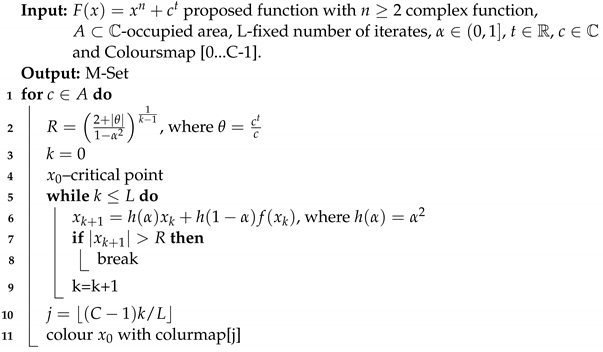 |
Mandelbrot Set
Here, we presented a discussion of several M-sets related to the function
at various n, within the trajectory of the suggested iteration. Here, M-sets have been generated for
via Mann-iteration with h-convexity. In every graph, we set
(i.e., number of iterations is fixed) in the Algorithm 1.
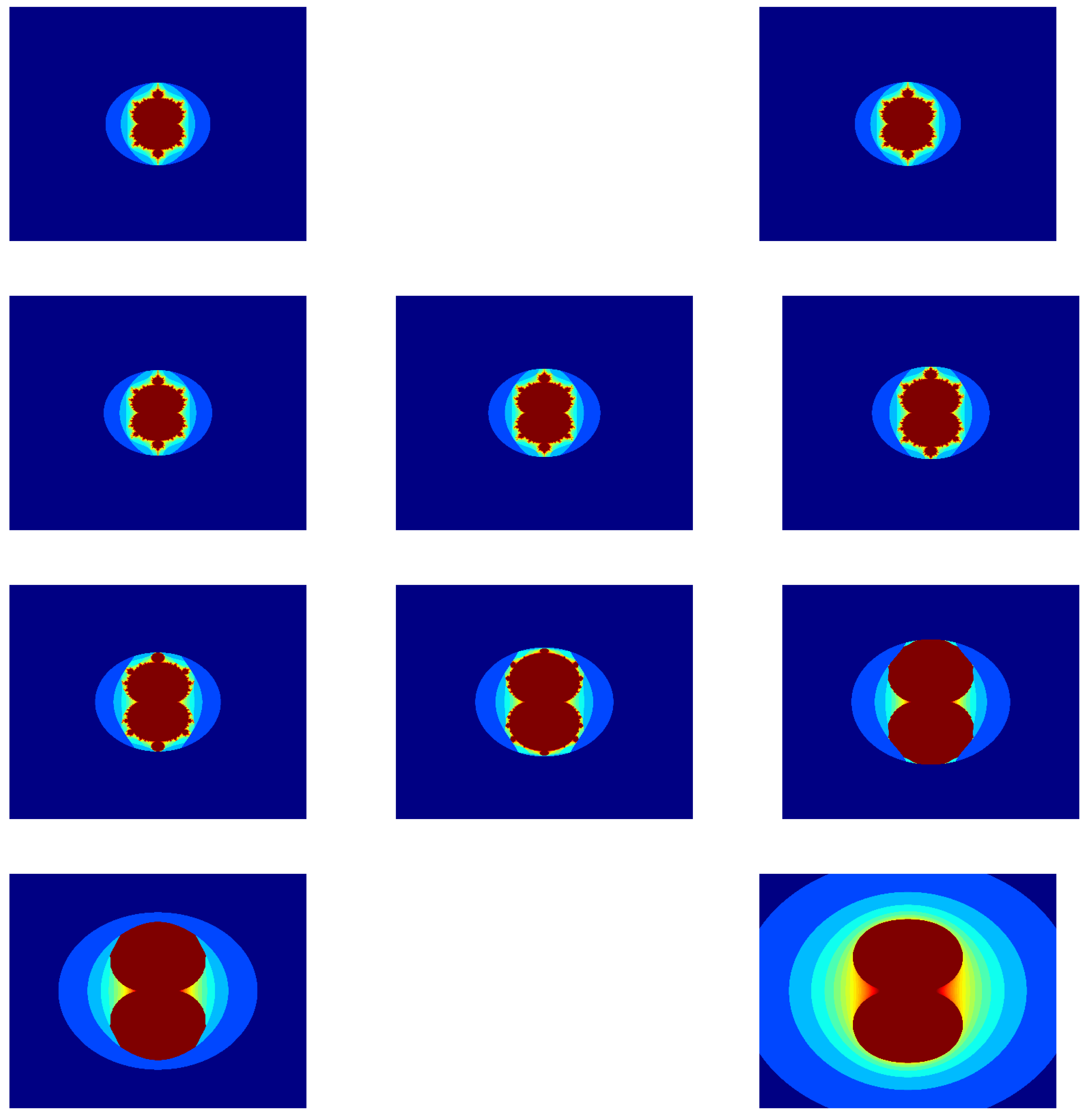
Example 1.
In Figure 1, we visualize how M-sets follow the function
at
by varying the other parameters to attain attractive M-sets.
Furthermore, in Figure 2 by fixing the parameter
and varying the value of the other parameters, we attain attractive M-sets using Mann iteration with h-convexity.
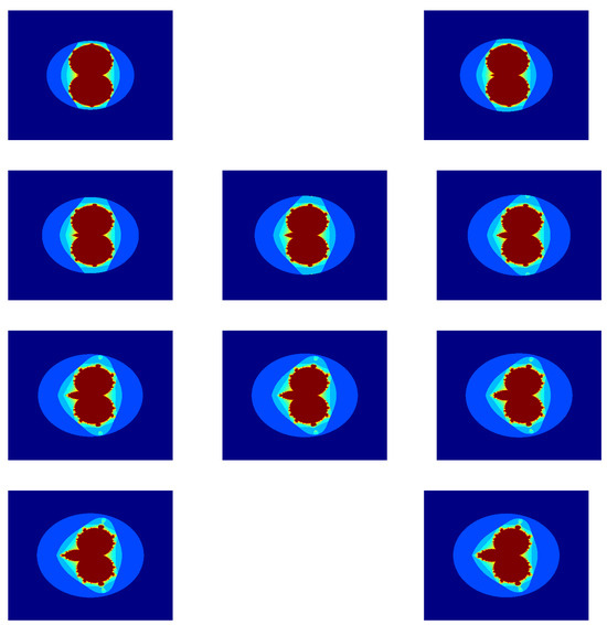
Figure 1.
M-set for
via the Mann-iterative scheme;
.
Figure 1.
M-set for
via the Mann-iterative scheme;
.
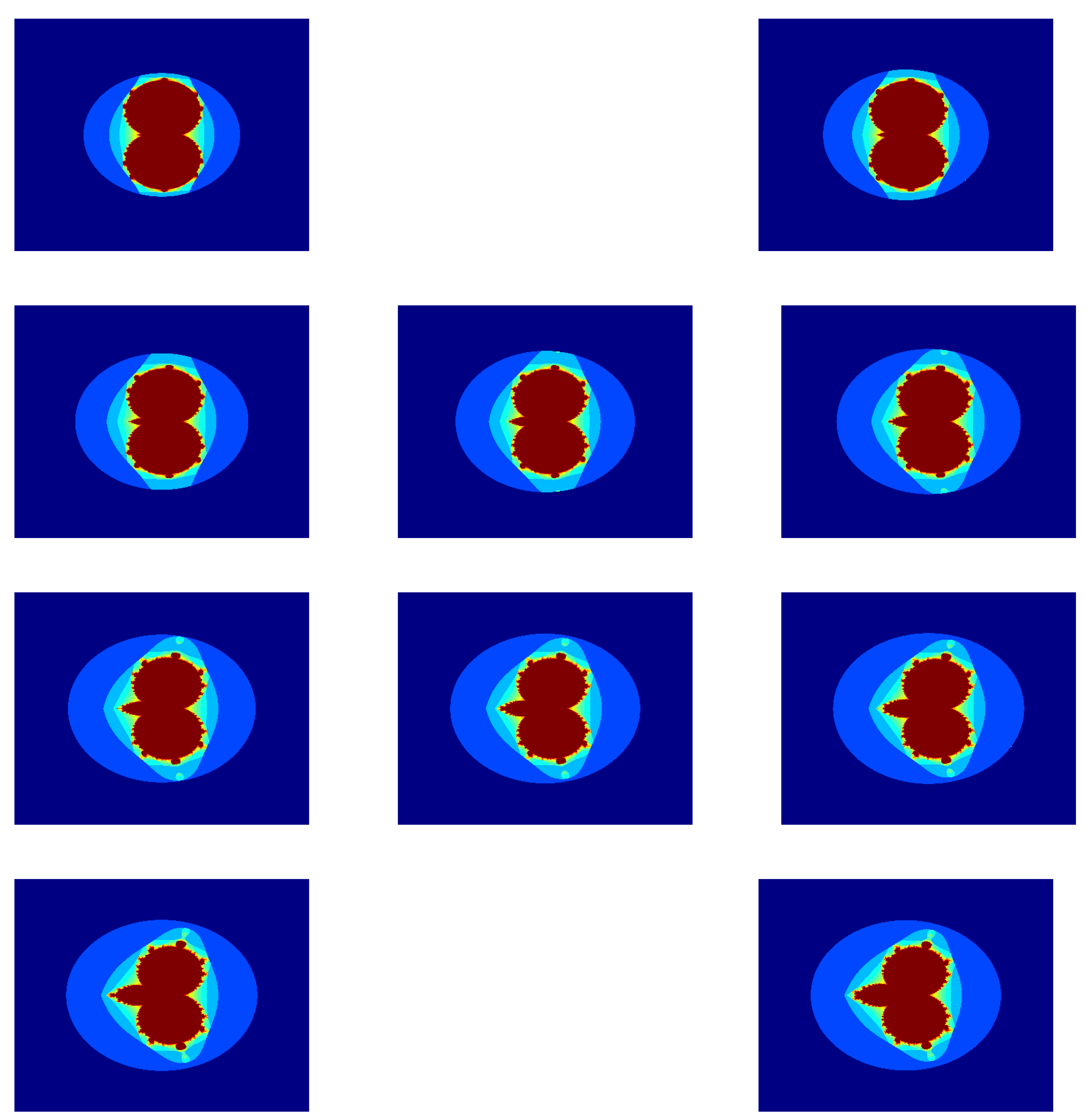
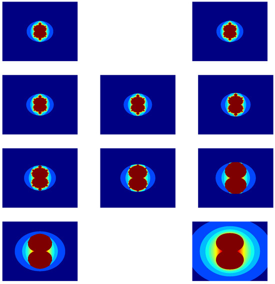
Figure 2.
M-set for
via the Mann-iterative scheme with h-convexity;
.
Figure 2.
M-set for
via the Mann-iterative scheme with h-convexity;
.
Example 2.
In Figure 3, we use the function
at
, and vary the other parameters to produce cubic M-sets using Mann iteration.
Moreover, in Figure 4, by fixing the parameter
and varying the other parameters to produce cubic M-sets using Mann iteration with h-convexity. It can be observed that the position of the parameter relative to the Mandelbrot set informs a lot about the polynomial’s dynamical properties. The Mandelbrot set is represented by a cubic polynomial
with two critical orbits. As a result, the apparel beauty of the Mandelbrot set using cubic polynomials
is far more intricate than quadratic polynomials
.
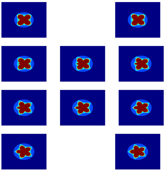
Figure 3.
M-set for
via the Mann-iterative scheme;
.
Figure 3.
M-set for
via the Mann-iterative scheme;
.
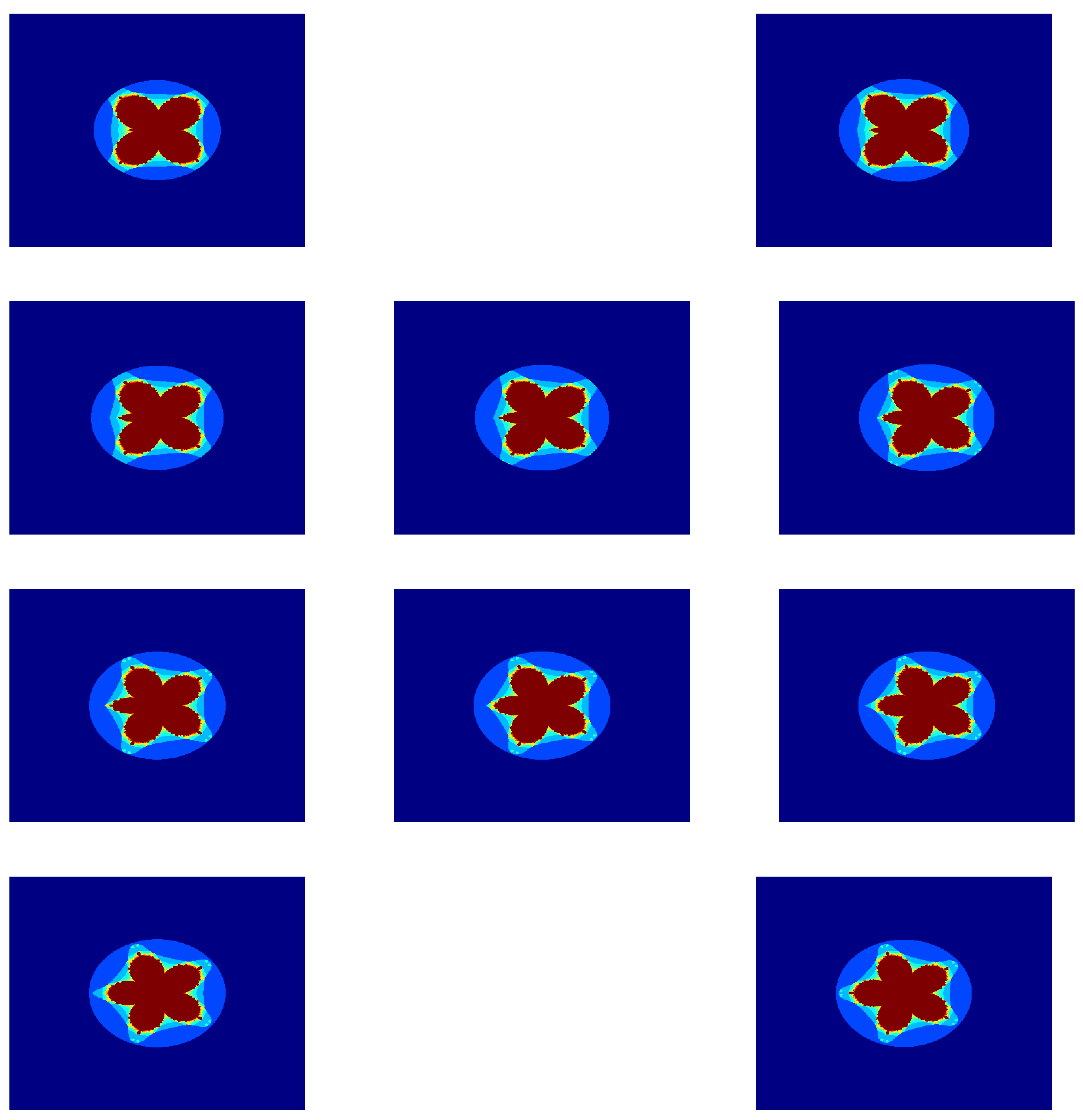
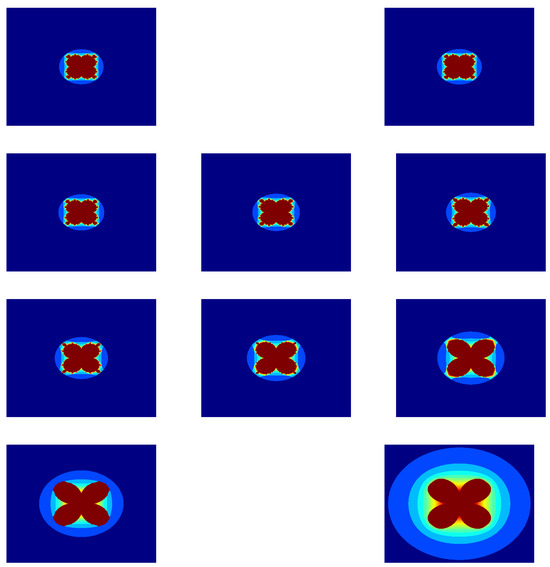
Figure 4.
M-set for
via the Mann-iterative scheme with h-convexity;
.
Figure 4.
M-set for
via the Mann-iterative scheme with h-convexity;
.
We continue this way, and discuss the following examples by considering various values of
and t for simple and convex functions. We observe the number of iterations and the amount of time to generate fractals.
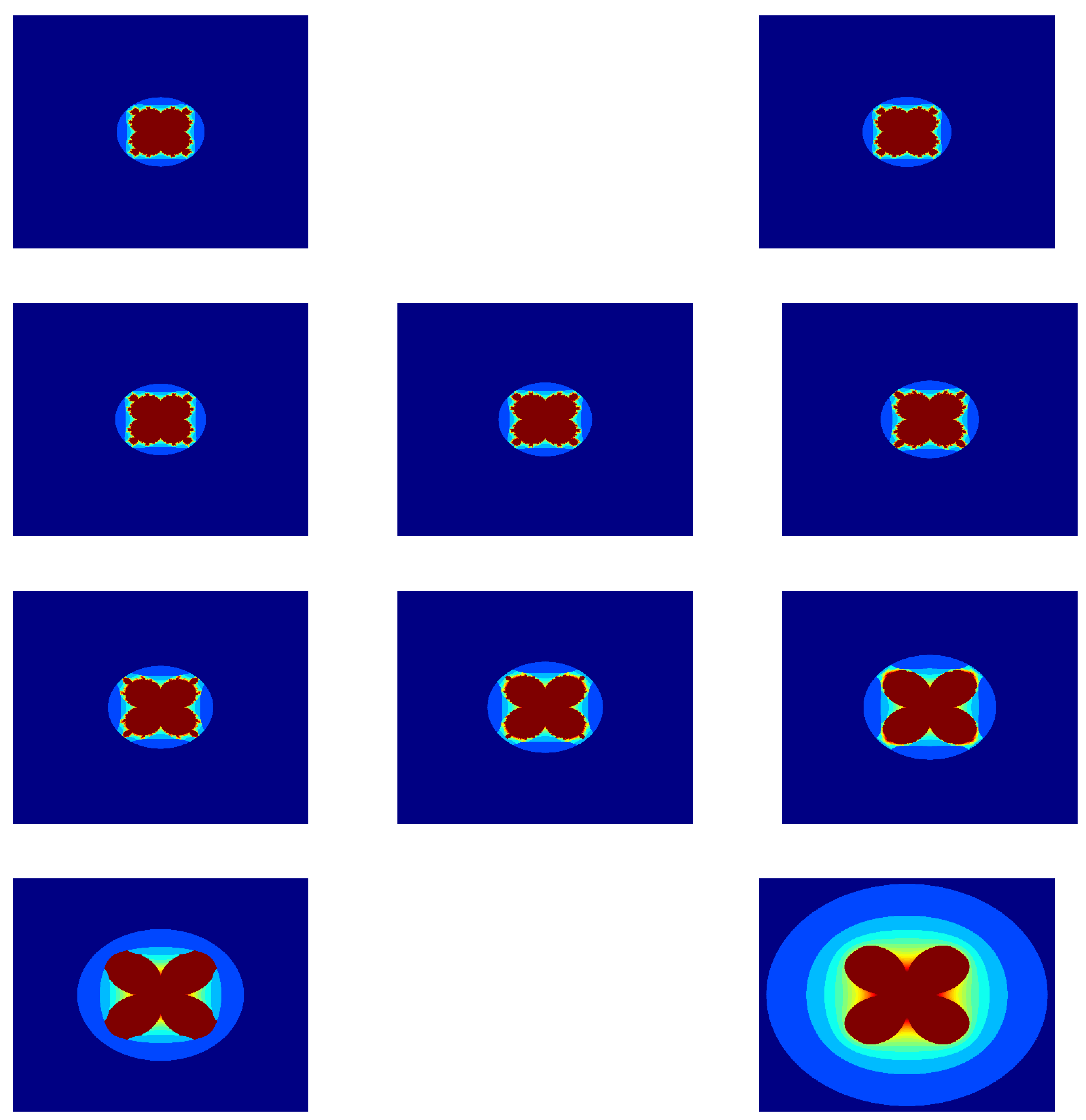
Example 3.

In the first ten figures of this example, we illustrate how the Mandelbrot sets follow the function
at
. In Figure 5, Figure 6, Figure 7, Figure 8, Figure 9, Figure 10, Figure 11, Figure 12, Figure 13 and Figure 14, we fix the parameter
and vary α to achieve visually appealing Mandelbrot sets. In these figures, the color bar represents the average number of iterations (ANI) required to generate each graph. It is evident from Table 1 that the Mann iterative scheme with h-convexity (MIH) outperforms the standard Mann iterative (MI) scheme.
Table 1.
Comparison table when
and
.
This table shows that the maximum number of iterations required for a simple Mann iteration is 810, which is significantly larger than 23 in the case of the proposed Mann iteration with h-convexity. Similarly, the time required to perform many iterations is also comparatively higher. Moreover, the images generated by our newly proposed Mann iteration with h-convexity are far better than the usual ones.
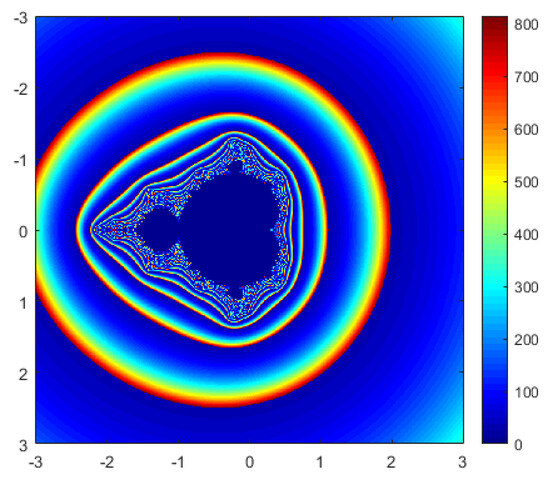
Figure 5.
M-set using MI for
.
Figure 5.
M-set using MI for
.
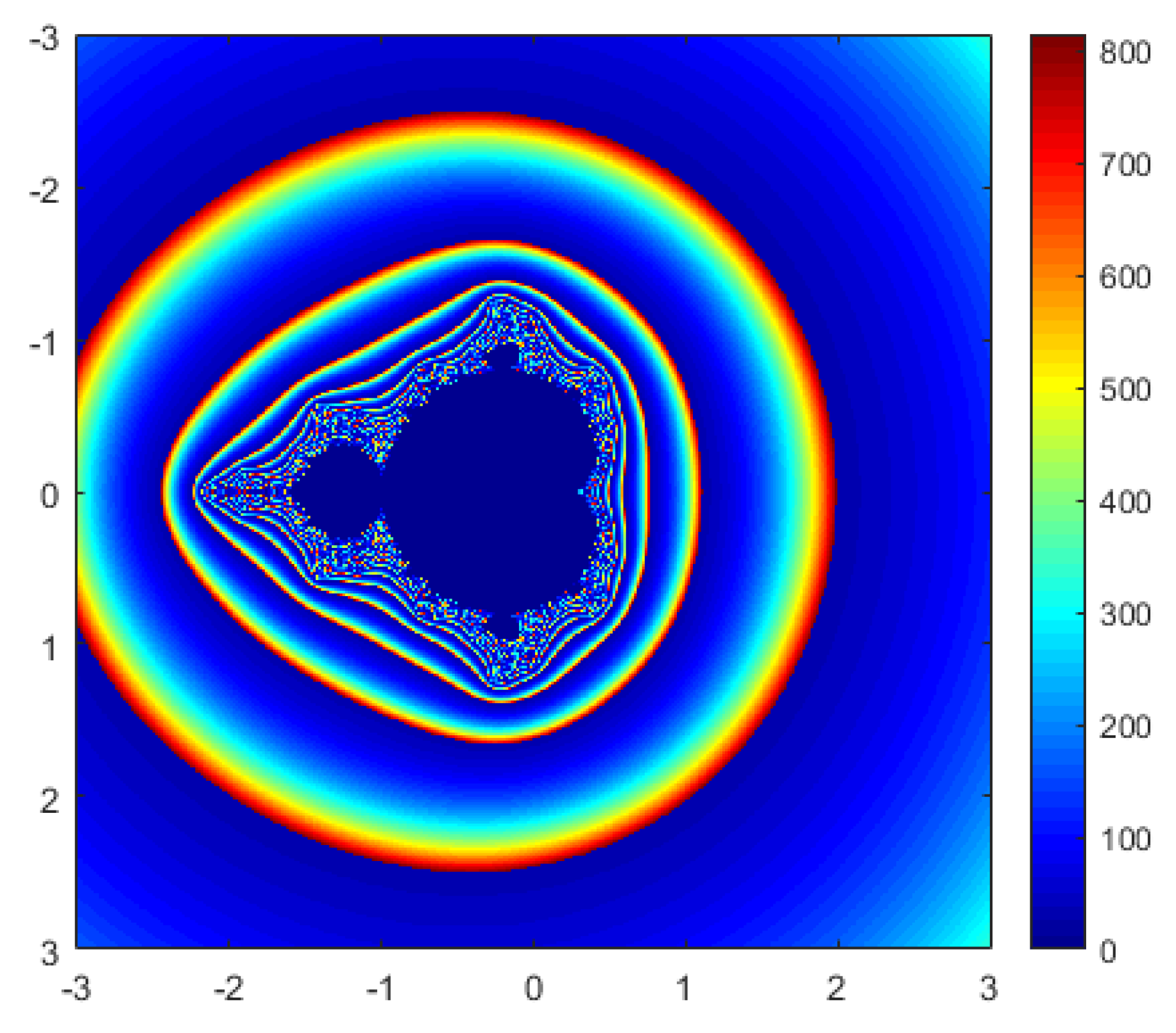
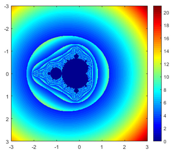
Figure 6.
M-set using MIH for
.
Figure 6.
M-set using MIH for
.
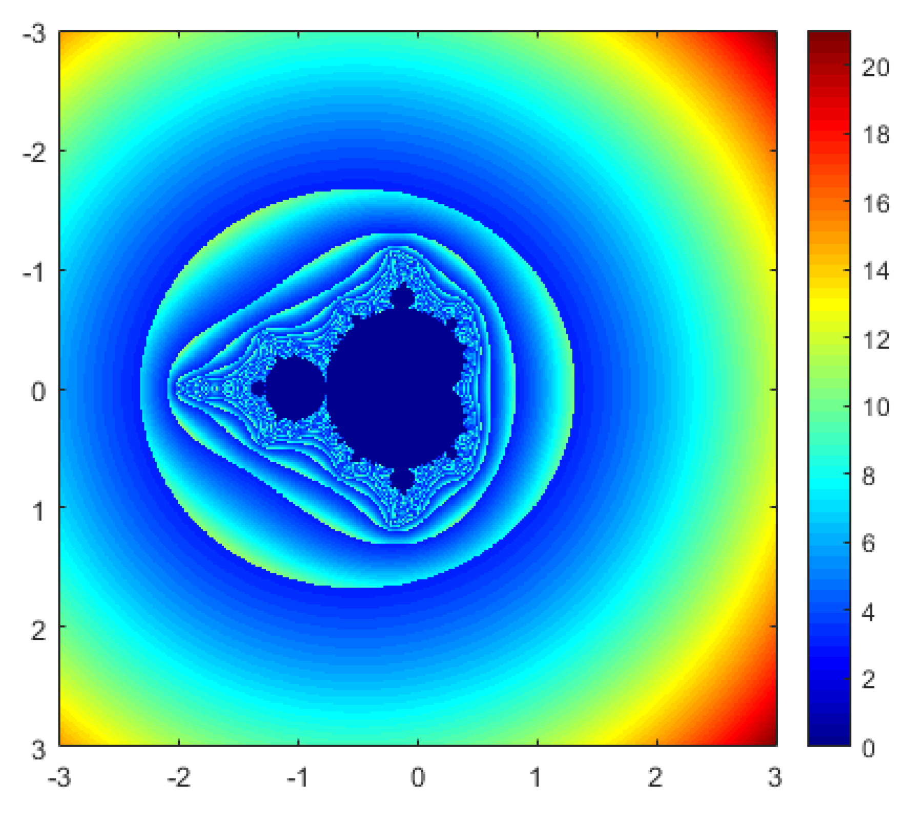

Figure 7.
M-set using MI for
.
Figure 7.
M-set using MI for
.
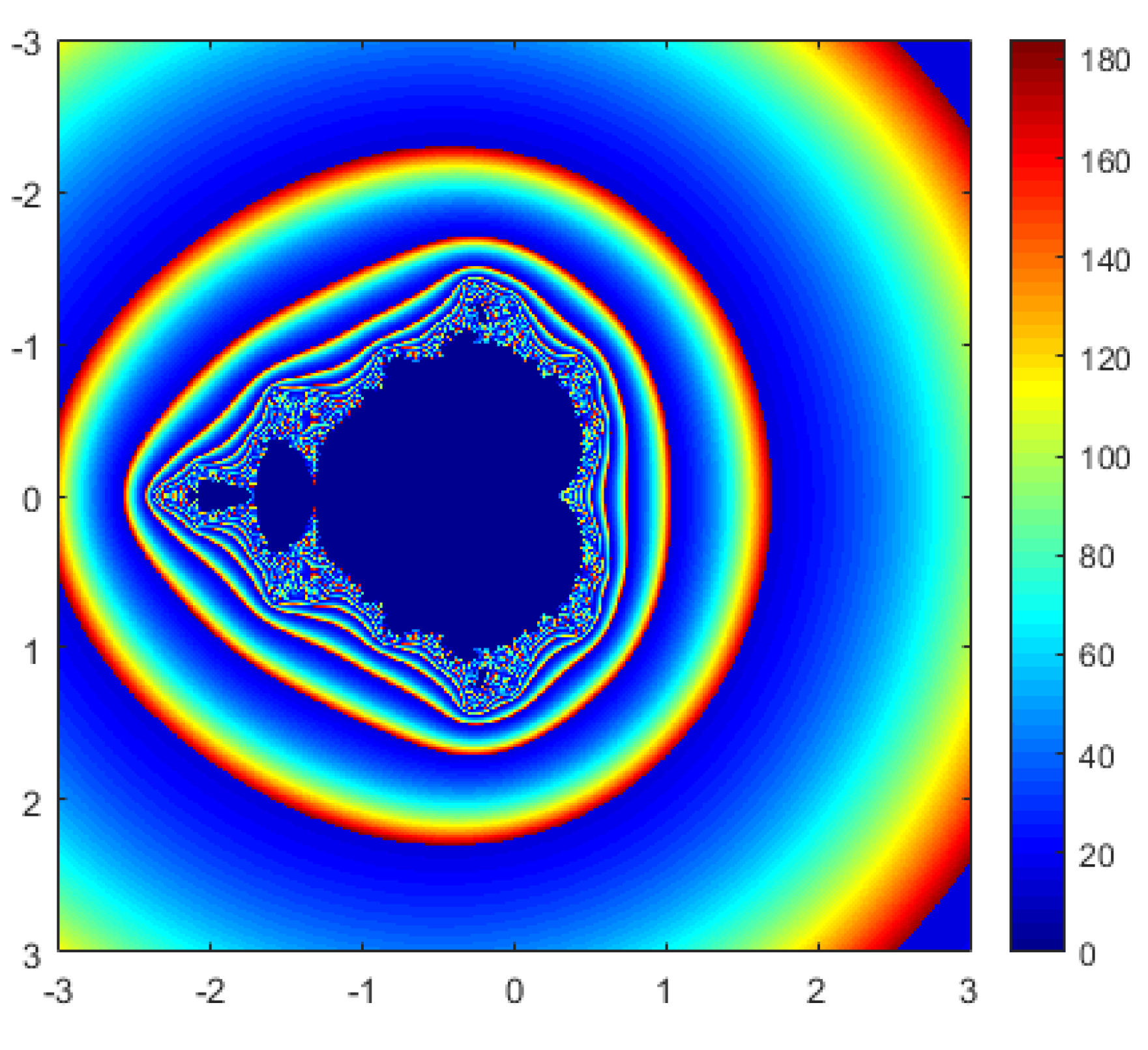
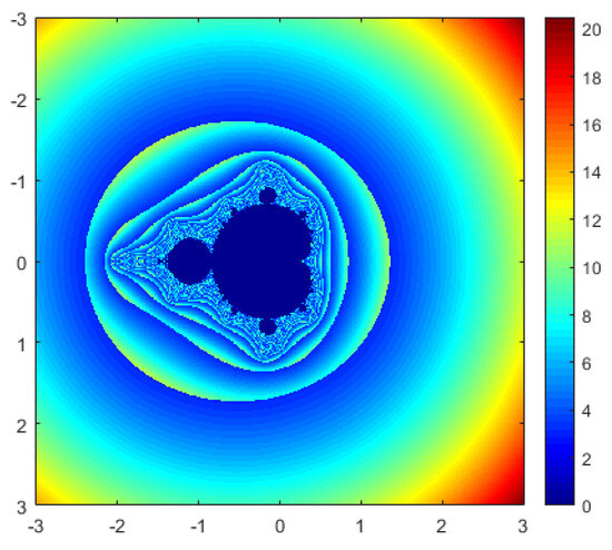
Figure 8.
M-set using MIH for
.
Figure 8.
M-set using MIH for
.
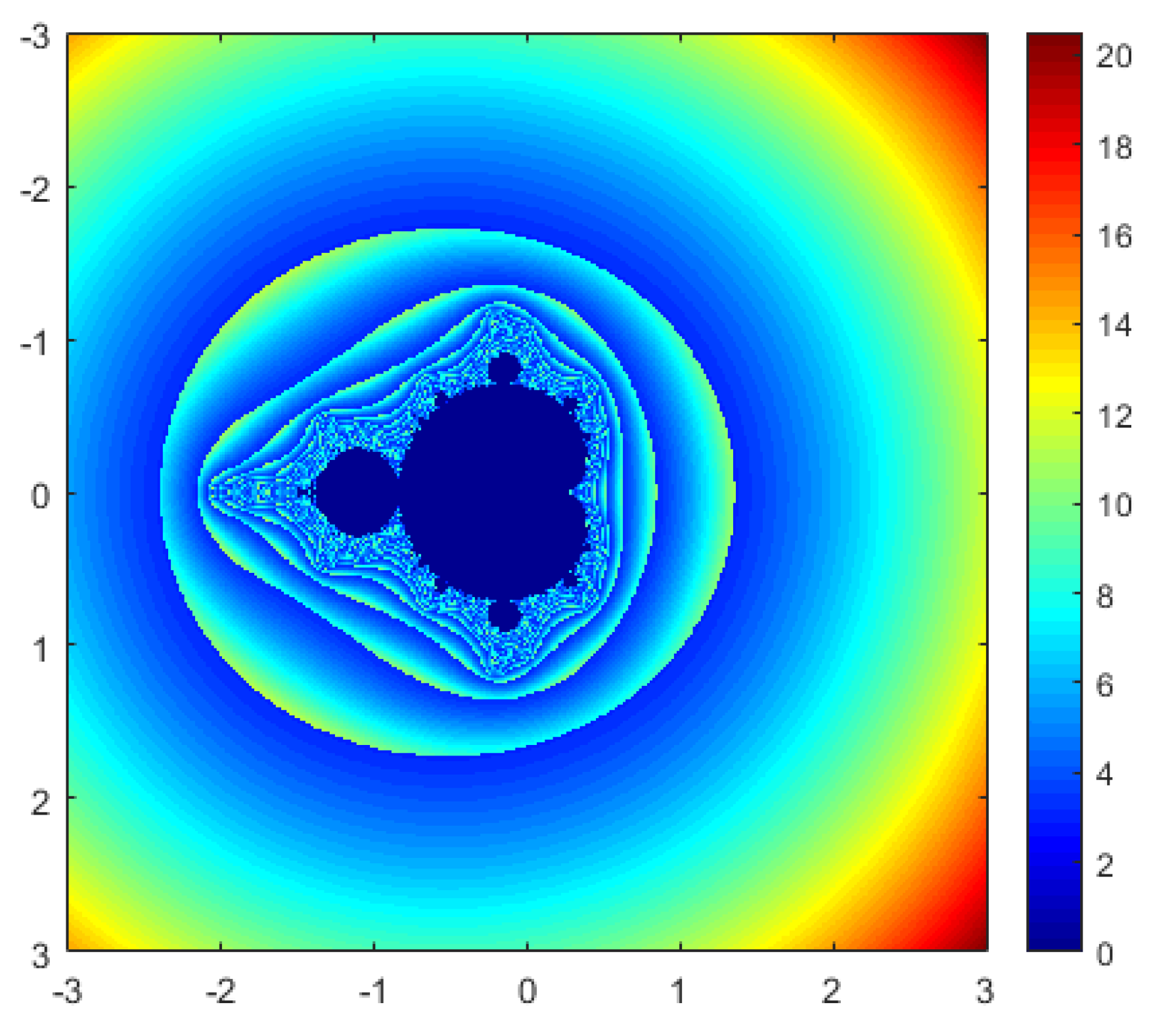

Figure 9.
M-set using MI for
.
Figure 9.
M-set using MI for
.
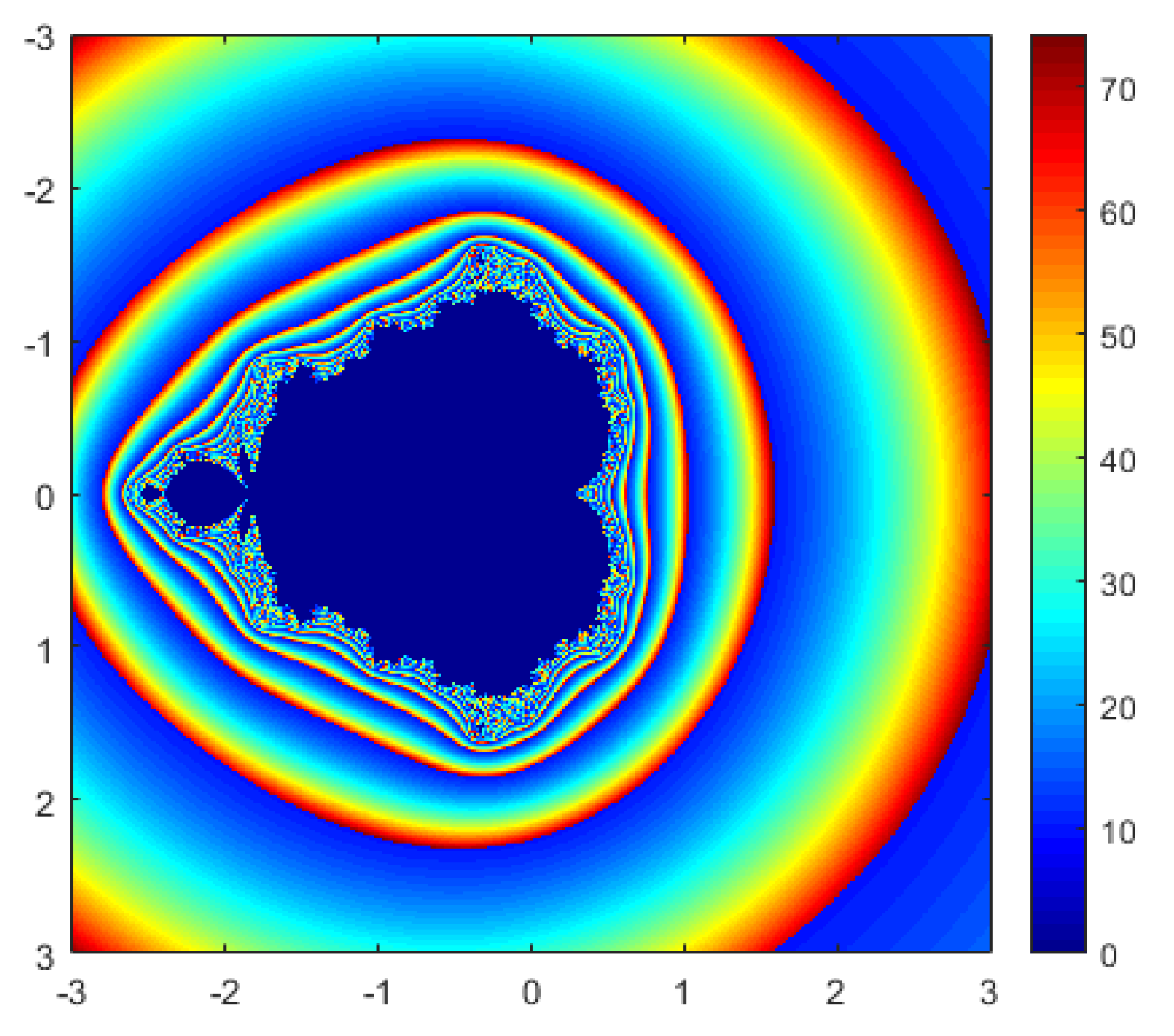

Figure 10.
M-set using MIH for
.
Figure 10.
M-set using MIH for
.
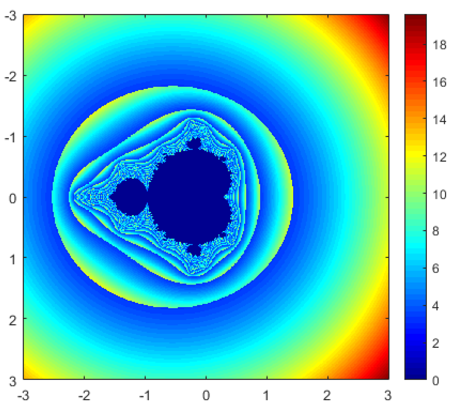

Figure 11.
M-set using MI for
.
Figure 11.
M-set using MI for
.
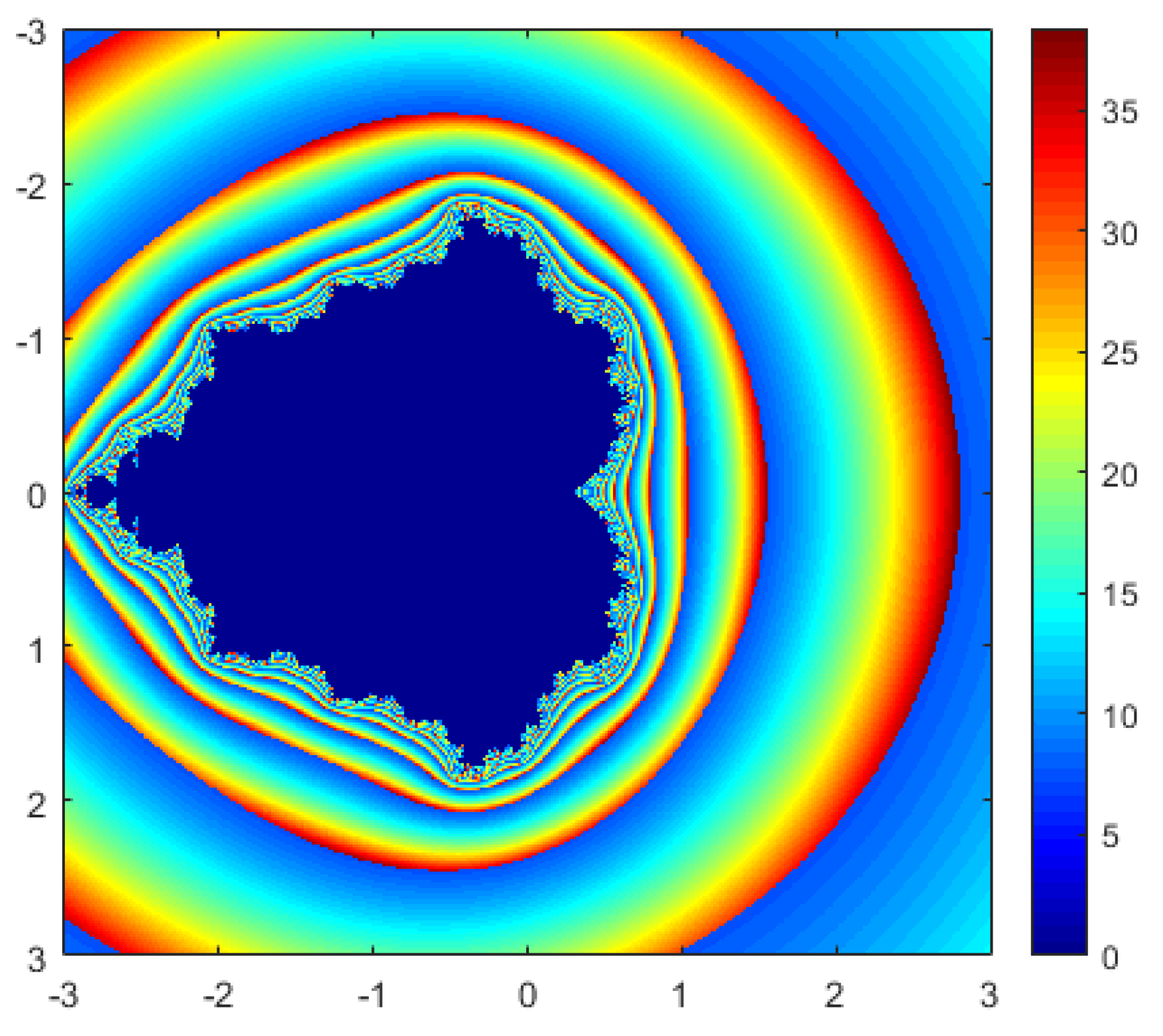
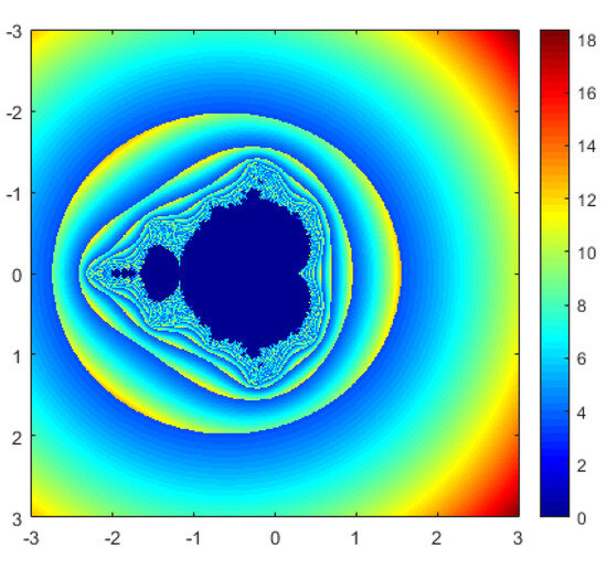
Figure 12.
M-set using MIH for
.
Figure 12.
M-set using MIH for
.
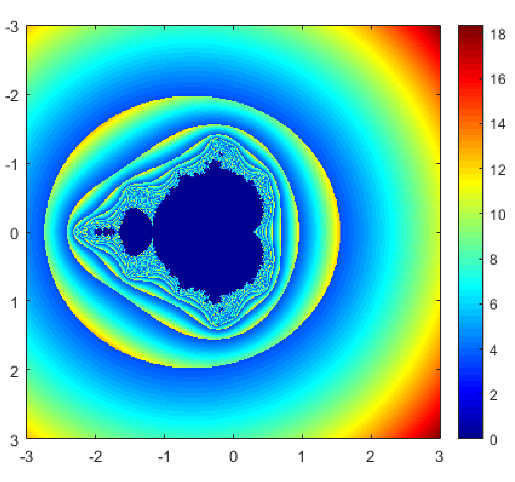

Figure 13.
M-set using MI for
.
Figure 13.
M-set using MI for
.
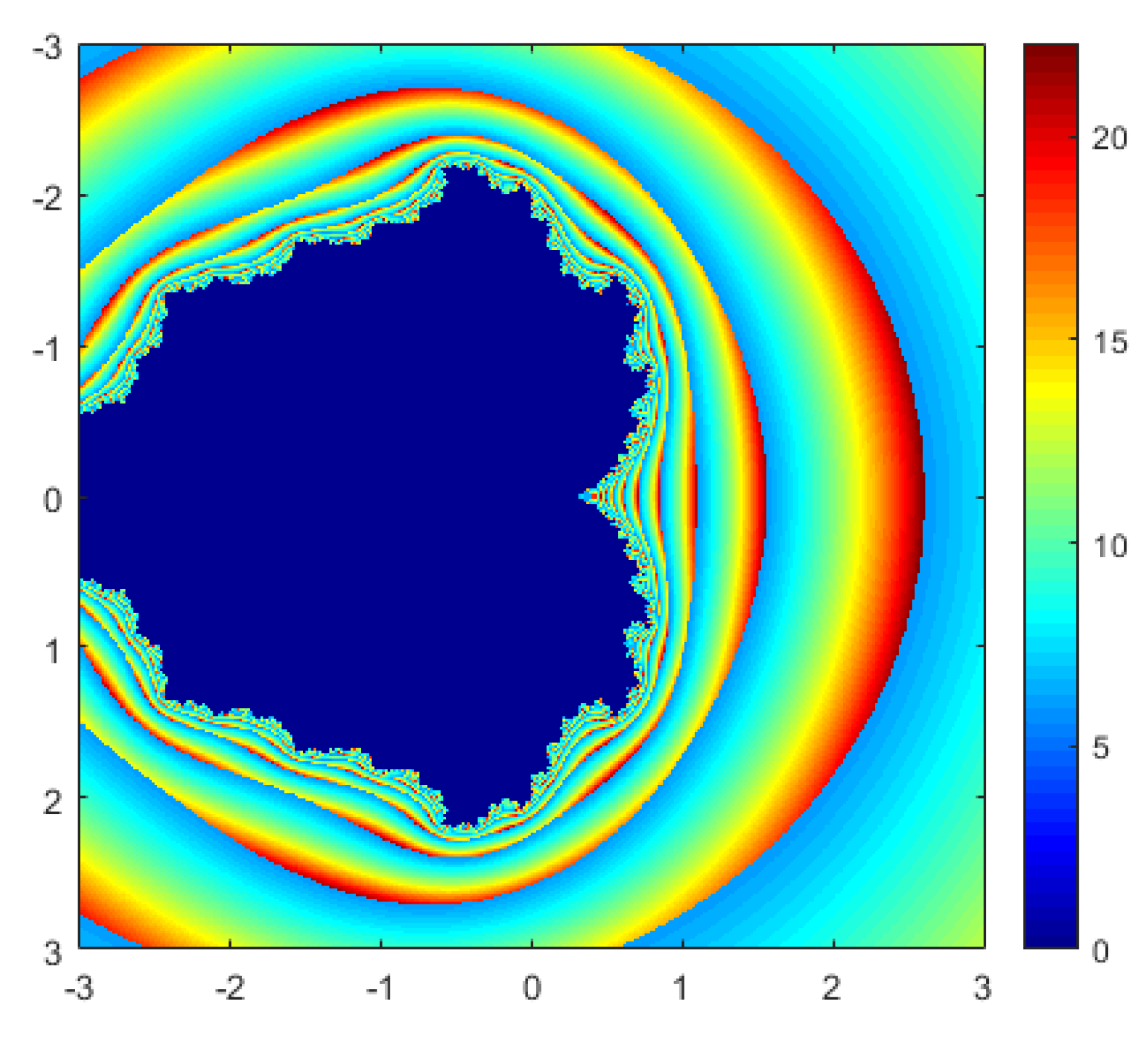
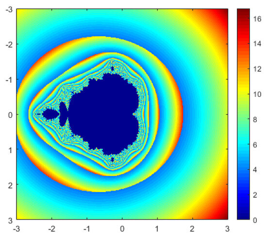
Figure 14.
M-set using MIH for
.
Figure 14.
M-set using MIH for
.

Example 4.
In the next figures, we demonstrate how the Mandelbrot sets correspond to the function
with
. This is shown in Figure 15, Figure 16, Figure 17, Figure 18, Figure 19, Figure 20, Figure 21, Figure 22, Figure 23 and Figure 24, where we fix the parameter
and vary the other parameter t to achieve visually appealing Mandelbrot sets. Again, from Table 2, we observe that the Mann iterative scheme with h-convexity outperforms the standard Mann scheme.
Table 2.
Comparison table when
and
.
This table shows that the maximum number of iterations required for a simple Mann iteration is 23,000, which is significantly larger than 100 in the case of the proposed Mann iteration with h-convexity. Similarly, the time required to perform many iterations is also comparatively higher. Moreover, the images generated by our newly proposed Mann iteration with h-convexity at
are far better than the usual ones.
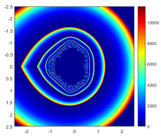
Figure 15.
M-set by using MI for
.
Figure 15.
M-set by using MI for
.
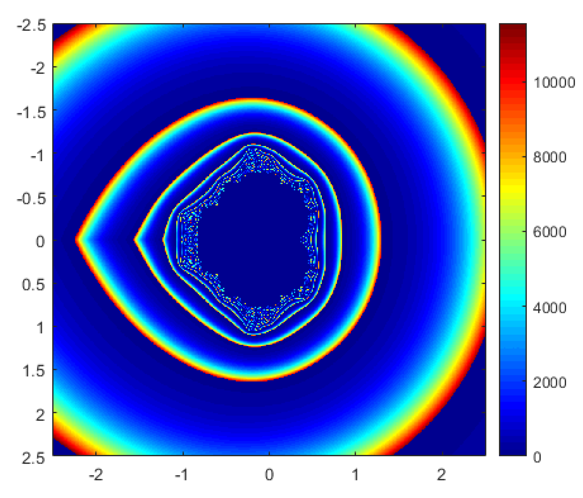
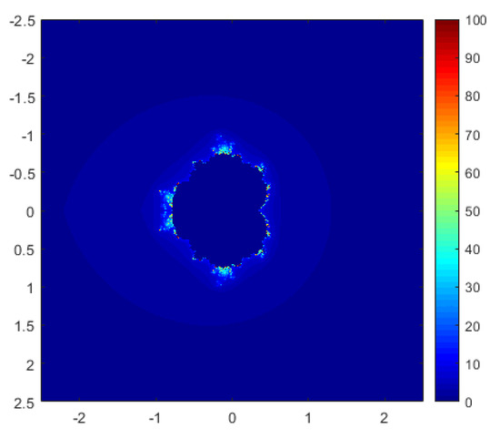
Figure 16.
M-set using MIH for
.
Figure 16.
M-set using MIH for
.


Figure 17.
M-set using MI for
.
Figure 17.
M-set using MI for
.
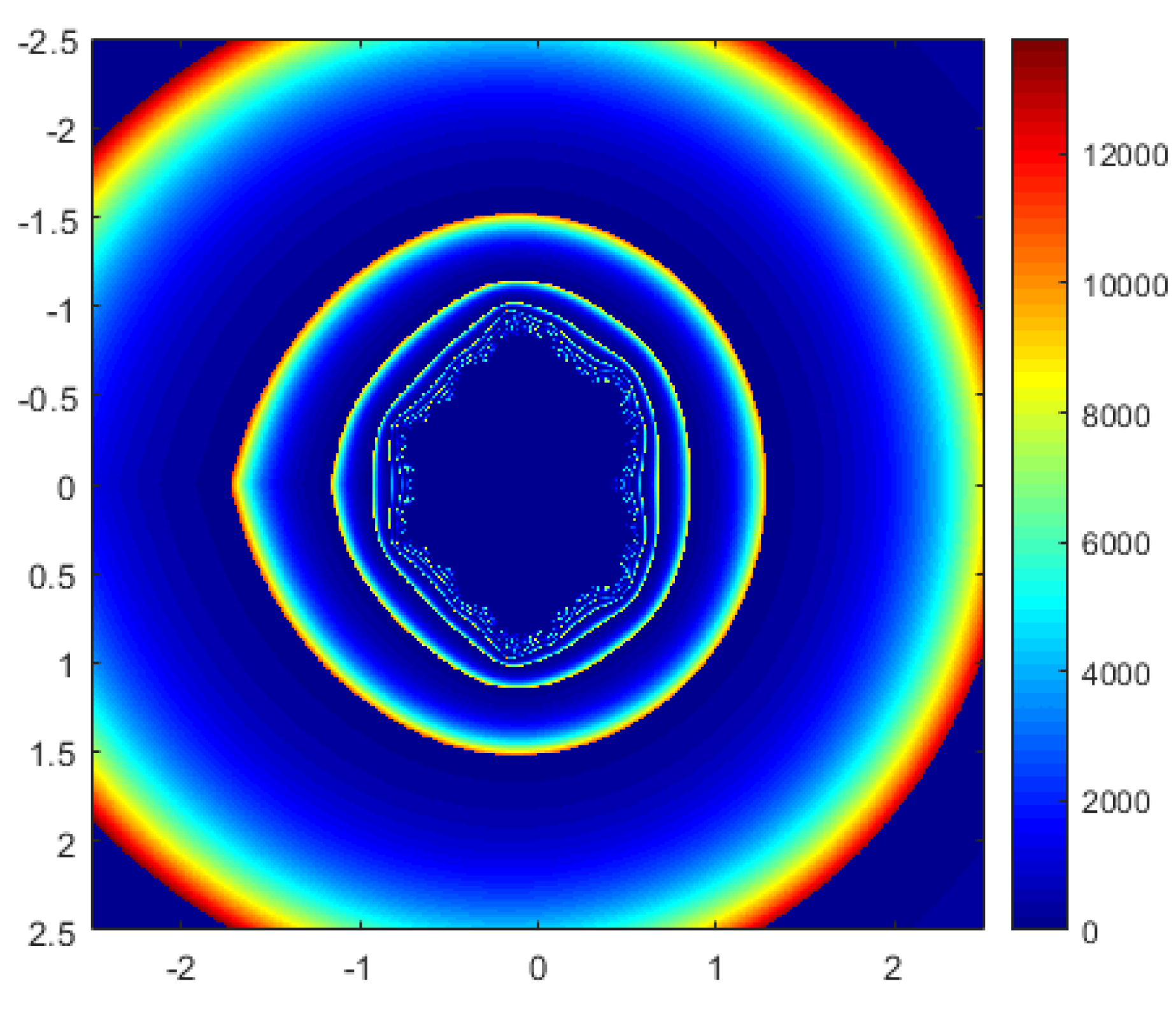
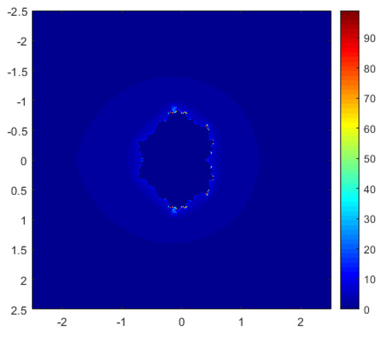
Figure 18.
M-set using MIH for
.
Figure 18.
M-set using MIH for
.

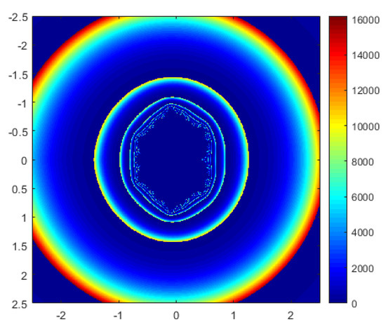
Figure 19.
M-set using MI for
.
Figure 19.
M-set using MI for
.
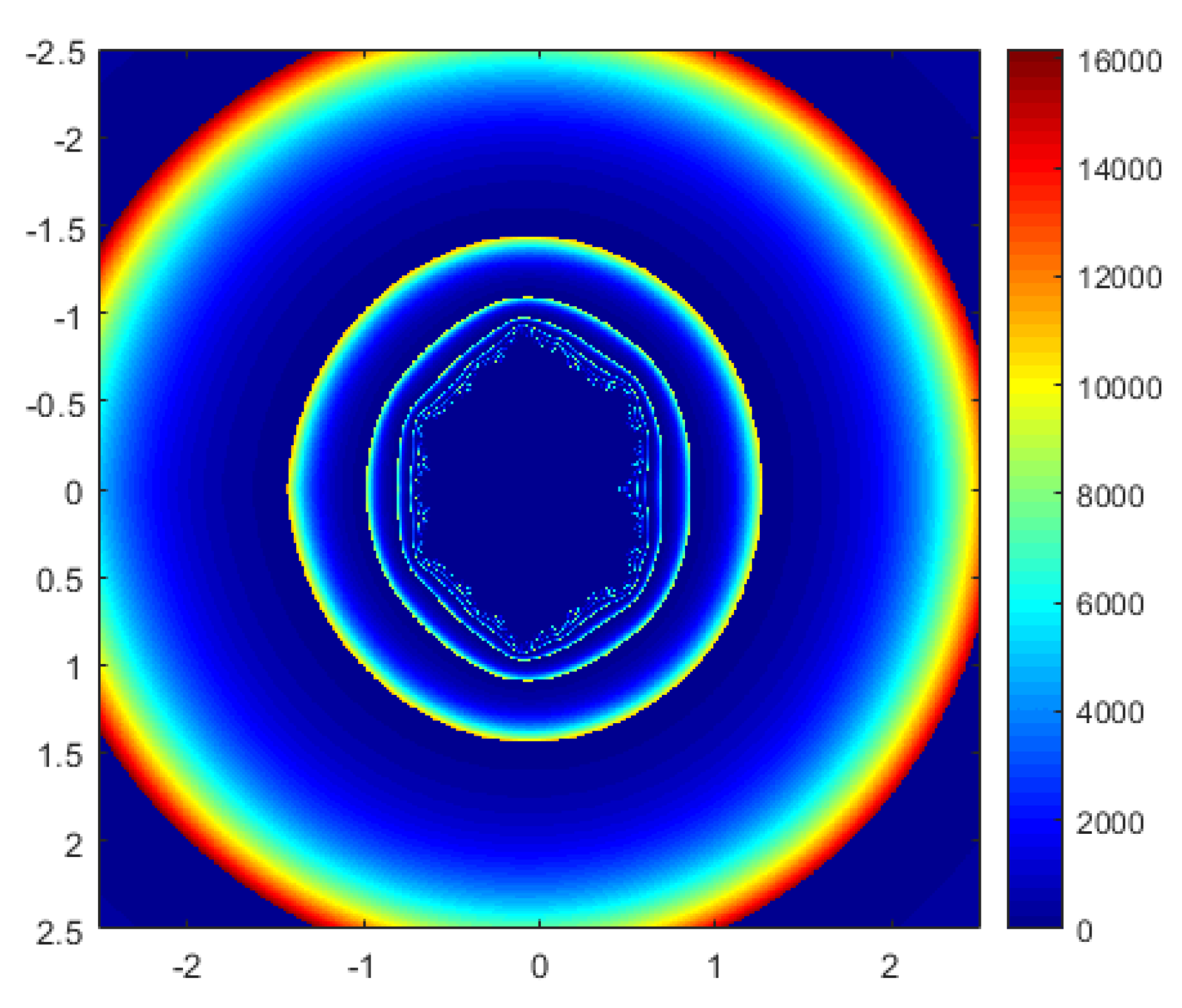

Figure 20.
M-set using MIH for
.
Figure 20.
M-set using MIH for
.
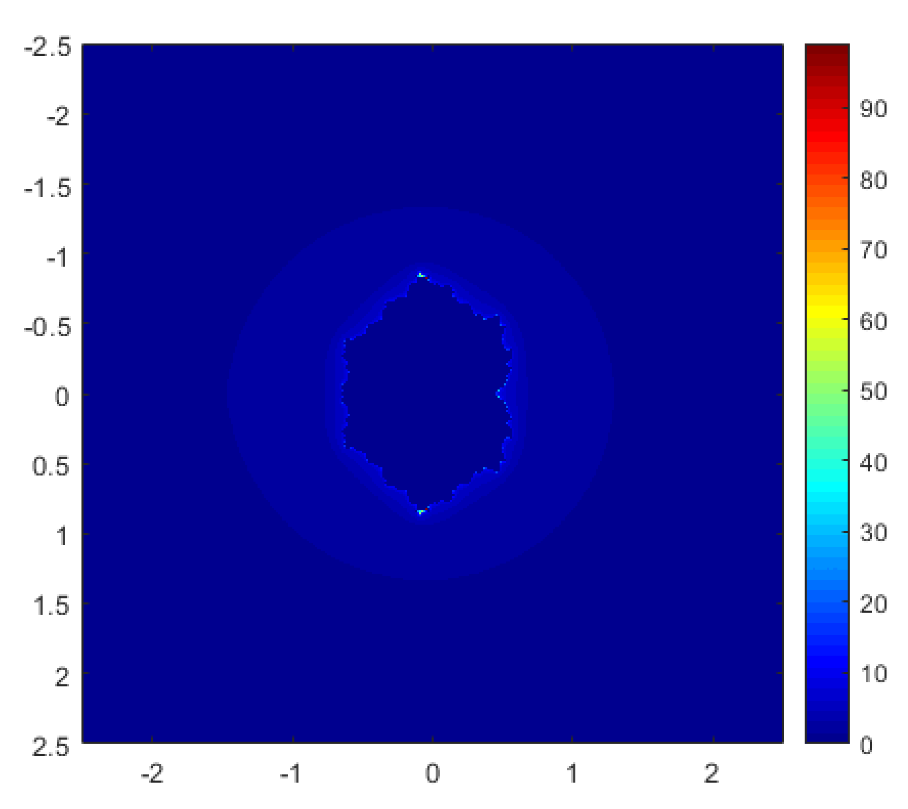
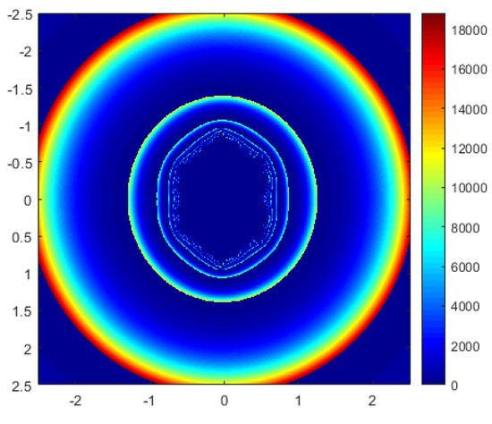
Figure 21.
M-set using MI for
.
Figure 21.
M-set using MI for
.


Figure 22.
M-set using MIH for
.
Figure 22.
M-set using MIH for
.
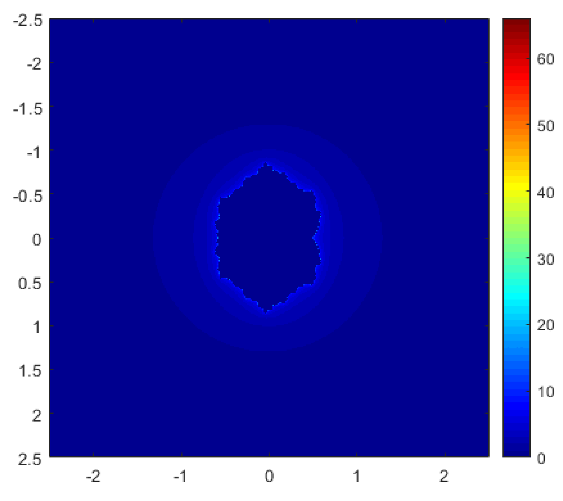

Figure 23.
M-set using MI for
.
Figure 23.
M-set using MI for
.
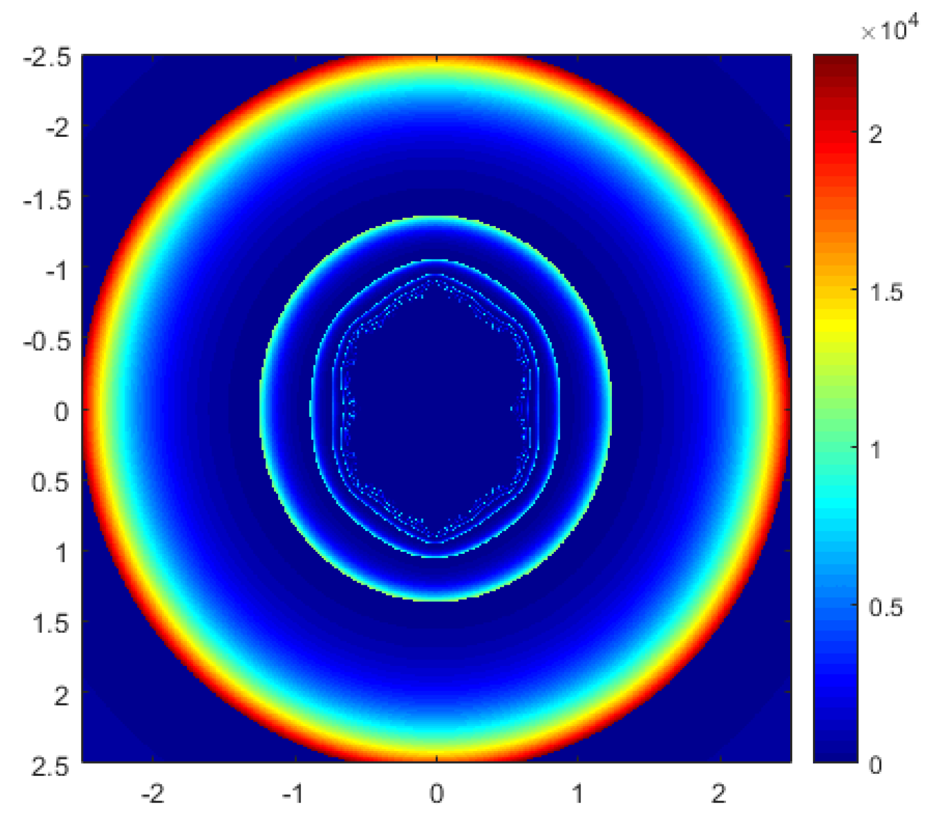
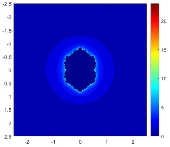
Figure 24.
M-set using MIH for
.
Figure 24.
M-set using MIH for
.

The Mandelbrot set, generated using the Mann-iterative scheme with h-convexity, holds significant potential across various scientific disciplines. Fractals, including the Mandelbrot set, are not merely mathematical curiosities; they provide profound insights and applications in several areas of science and technology, such as natural phenomena and geophysics, art and design, physics, biology and medicine, materials science and engineering, computer graphics and image processing, chaos theory and dynamical systems. Highlighting such significance, these findings will also be a road to quixotic research in diverse directions such as using fractal dimension analysis to describe the three-dimensional association of biomolecules. Such insights have incredible potential to transform the modeling and understanding of essential developments in biophysics [43].
5. Further Discussion and Conclusions
We introduced the Mann orbit with h-convexity and established a novel escape criterion for a complex function
, where
, c belongs to the set of complex numbers, and t is a real number. Our work resulted in Algorithm 1 for generating Mandelbrot sets. We provided detailed presentations of quadratic and cubic fractals, particularly Mandelbrot sets, with illustrative examples. Our comparative analysis, as demonstrated in the previous examples, consistently shows that the Mann iterative scheme with h-convexity outperforms the standard Mann iterative scheme because MIH takes less time and generates higher-quality fractals as compared to the MI.
Analyzing the relationship between the Mandelbrot set and the input parameters of iteration is extremely intricate. In this part, we visualized the graphs of the Mandelbrot set through the implementation of escape time algorithm for the Mann iterative scheme with h-convexity and we investigated the variation in the average visual time required for execution by adjusting two factors
for Mann iterative scheme with h-convexity. We expressed the parameters
and
as intervals for further analysis. To obtain the desired outcomes, we perform calculations for both “
” and “t” using a step size of 0.01 within each interval. In total, we compute 100 values for “
” and 100 values for “t”. It should be noted that all calculations and visual analyses were performed on a computer equipped with the following configuration: an Intel(R) Core(TM) i7-7500U CPU running at 2.70 GHz, 8 GB of RAM, and a 64-bit Windows 10 Pro Education operating system. To determine the mean image processing time, we employed Mathematica 10 software and executed the algorithm. Investigating the influence of input parameters t and
on the Mandelbrot set during the Mann-iteration with h-convexity orbit, we fixed the number of iterations at 15. The color map used to depict the time values was constrained within the interval of 4.287 to 43.858 s. The visualization uncovers intriguing insights into the execution time of the algorithm when applied to various parameter values in Figure 25.
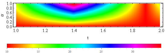
Figure 25.
M-set for
via Mann-iterative scheme having image visual period.
Overall, our research lays the foundation for the further exploration and development of iterative schemes for fractal generation, with potential applications in various scientific, artistic, and computational fields. It is remarkable that usually, for h-convex functions, researchers use
or
, but in this study, we use
to generalize the Mann-iterative scheme.
Author Contributions
Conceptualization, A.T. and M.T.; Data curation, M.Z. and M.A.; Formal analysis, A.T., M.A. and M.T.; Investigation, A.T., C.C. and M.T.; Methodology, A.T., M.T. and M.A.; Project administration, M.Z. and C.C.; Resources, M.A. and C.C.; Supervision, C.C.; Validation, C.C.; writing—original draft preparation, A.T., M.T., M.Z., M.A., and C.C. Writing—review and editing, M.T., C.C. and M.A. All authors have read and agreed to the published version of the manuscript.
Funding
No specific external funding has been received for this article.
Data Availability Statement
The research is theoretical in nature. As a result, no data were used.
Acknowledgments
The author extends the appreciation to the Deanship of Postgraduate Studies and Scientific Research at Majmaah University for funding this research work through the project number (ER-2024-1193).
Conflicts of Interest
The authors declare that they have no competing interests.
Abbreviations
The following abbreviations are used in this manuscript:
| M-Set | Mandelbrot set |
| J-Set | Julia set |
| ANI | Average number of iterations |
| MI | Mann-iterative scheme |
| MIH | Mann-iterative scheme with h-convexity |
References
- Barnsley, M. Fractals Everywhere; Academic: Boston, MA, USA, 1993. [Google Scholar]
- Taylor, R.P. The potential of biophilic fractal designs to promote health and performance: A review of experiments and applications. Sustainability 2021, 13, 823. [Google Scholar] [CrossRef]
- Smith, J.; Rowland, C.; Moslehi, S.; Taylor, R.; Lesjak, A.; Lesjak, M.; Stadlober, S.; Lee, L.; Dettmar, J.; Page, M.; et al. Relaxing floors: Fractal fluency in the built environment. Nonlinear Dyn. Psychol. Life Sci. 2020, 24, 127–141. [Google Scholar]
- Fisher, Y. Fractal image compression. Fractals 1994, 2, 347–361. [Google Scholar] [CrossRef]
- Kumar, S. Public key cryptographic system using Mandelbrot sets. In Proceedings of the MILCOM 2006—2006 IEEE Military Communications Conference, Washington, DC, USA, 23–25 October 2006; pp. 1–5. [Google Scholar]
- Zhang, X.; Wang, L.; Zhou, Z.; Niu, Y. A chaos-based image encryption technique utilizing Hilbert curves and H-Fractals. IEEE Access 2019, 7, 74734–74746. [Google Scholar] [CrossRef]
- Kharbanda, M.; Bajaj, N. An exploration of fractal art in fashion design. In Proceedings of the 2013 International Conference on Communication and Signal Processing, Melmaruvathur, India, 3–5 April 2013; pp. 226–230. [Google Scholar]
- Cohen, N. Fractal antenna applications in wireless telecommunications. In Proceedings of the Professional Program Proceedings. Electronic Industries Forum of New England, Boston, MA, USA, 6–8 May 1997; pp. 43–49. [Google Scholar]
- Mandelbrot, B.B. The Fractal Geometry Nature; Freeman: New York, NY, USA, 1982; Volume 2. [Google Scholar]
- Lakhtakia, A.; Varadan, W.; Messier, R.; Varadan, V.K. On the symmetries of the Julia sets for the process zp+c. J. Phys. A Math. Gen. 1987, 20, 3533–3535. [Google Scholar] [CrossRef]
- Blanchard, P.; Devaney, R.L.; Garijo, A.; Russell, E.D. A generalized version of the Mcmullen domain. Int. J. Bifurc. Chaos 2008, 18, 2309–2318. [Google Scholar] [CrossRef]
- Crowe, W.D.; Hasson, R.; Rippon, P.J.; Strain-Clark, P.E.D. On the structure of the Mandelbar set. Nonlinearity 1989, 2, 541. [Google Scholar] [CrossRef]
- Kim, T. Quaternion Julia set shape optimization. Comput. Graph. Forum 2015, 34, 167–176. [Google Scholar] [CrossRef]
- Drakopoulos, V.; Mimikou, N.; Theoharis, T. An overview of parallel visualisation methods for Mandelbrot and Julia sets. Comput. Graph. 2003, 27, 635–646. [Google Scholar] [CrossRef]
- Sun, Y.; Chen, L.; Xu, R.; Kong, R. An image encryption algorithm utilizing Julia sets and Hilbert curves. PLoS ONE 2014, 9, e84655. [Google Scholar] [CrossRef]
- Prasad, B.; Katiyar, K. Fractals via Ishikawa iteration. In Proceedings of the International Conference on Logic, Information, Control and Computation, Gandhigram, India, 25–27 February 2011; pp. 197–203. [Google Scholar]
- Rani, M.; Agarwal, R. Effect of stochastic noise on superior Julia sets. J. Math. Imag. Vis. 2010, 36, 63. [Google Scholar] [CrossRef]
- Ashish, M.R.; Chugh, R. Julia sets and mandelbrot sets in Noor orbit. Appl. Math. Comput. 2014, 228, 615–631. [Google Scholar] [CrossRef]
- Kang, S.M.; Rafiq, A.; Latif, A.; Shahid, A.A.; Kwun, Y.C. Tricorns and Multi-corns of S-iteration scheme. J. Funct. Spaces 2015, 2015, 1–7. [Google Scholar]
- Tassaddiq, A.; Tanveer, M.; Azhar, M.; Lakhani, F.; Nazeer, W.; Afzal, Z. Escape criterion for generating fractals using Picard–Thakur hybrid iteration. Alex. Eng. J. 2024, 100, 331–339. [Google Scholar] [CrossRef]
- Tassaddiq, A.; Tanveer, M.; Azhar, M.; Nazeer, W.; Qureshi, S. A Four Step Feedback Iteration and Its Applications in Fractals. Fractal Fract. 2023, 7, 662. [Google Scholar] [CrossRef]
- Goyal, K.; Prasad, B. Dynamics of iterative schemes for quadratic polynomial. Proc. AIP Conf. 2001, 9, 149–153. [Google Scholar]
- Tassaddiq, A.; Tanveer, M.; Israr, K.; Arshad, M.; Shehzad, K.; Srivastava, R. Multicorn Sets of (¯z)k+cm via S-Iteration with h-Convexity. Fractal Fract. 2023, 7, 486. [Google Scholar] [CrossRef]
- Chugh, R.; Kumar, V.; Kumar, S. Strong convergence of a new three step iterative scheme in Banach spaces. Am. J. Comput. Math. 2012, 2, 345. [Google Scholar] [CrossRef]
- Phuengrattana, W.; Suantai, S. On the rate of convergence of Mann, Ishikawa, Noor and SP-iterations for continuous functions on an arbitrary interval. J. Comput. Appl. Math. 2011, 235, 3006–3014. [Google Scholar] [CrossRef]
- Tassaddiq, A.; Kalsoom, A.; Rashid, M.; Sehr, K.; Almutairi, D.K. Generating Geometric Patterns Using Complex Polynomials and Iterative Schemes. Axioms 2024, 13, 204. [Google Scholar] [CrossRef]
- Srivastava, R.; Tassaddiq, A.; Kasmani, R.M. Escape Criteria Using Hybrid Picard S-Iteration Leading to a Comparative Analysis of Fractal Mandelbrot Sets Generated with S-Iteration. Fractal Fract. 2024, 8, 116. [Google Scholar] [CrossRef]
- Li, D.; Tanveer, M.; Nazeer, W.; Guo, X. Boundaries of filled Julia sets in generalized Jungck-Mann orbit. IEEE Access 2019, 7, 76859–76867. [Google Scholar] [CrossRef]
- Tassaddiq, A. General escape criteria for the generation of fractals in extended Jungck-Noor orbit. Math. Comput. Simul. 2022, 196, 1–14. [Google Scholar] [CrossRef]
- Gdawiec, K.; Kotarski, W.; Lisowska, A. Biomorphs via modified iterations. J. Nonlinear Sci. Appl. 2016, 9, 2305–2315. [Google Scholar] [CrossRef]
- Pickover, C.A. Biomorphs: Computer displays of biological forms generated from mathematical feedback loops. Comput. Graph. Forum 1986, 5, 313–316. [Google Scholar] [CrossRef]
- Alonso-Sanz, R. Biomorphs with memory. Int. J. Parallel Emergent Distrib. Syst. 2018, 33, 1–11. [Google Scholar] [CrossRef]
- Jakubska-Busse, A.; Janowicz, M.W.; Ochnio, L.; Ashbourn, J.M.A. Pickover biomorphs and non-standard complex numbers. Chaos Solitons Fractals 2018, 113, 46–52. [Google Scholar] [CrossRef]
- Devaney, R. A First Course in Chaotic Dynamical Systems: Theory and Experiment; Addison-Wesley: New York, NY, USA, 1992. [Google Scholar]
- Liu, X.; Zhu, Z.; Wang, G.; Zhu, W. Composed accelerated escape time algorithm to construct the general Mandelbrot sets. Fractals 2001, 9, 149–153. [Google Scholar] [CrossRef]
- Mann, W.R. Mean value methods in iteration. Proc. Amer. Math. Soc. 1953, 4, 506–510. [Google Scholar] [CrossRef]
- Ishikawa, S. Fixed points by a new iteration method. Proc. Amer. Math.Soc. 1974, 44, 147–150. [Google Scholar] [CrossRef]
- Varoanec, S. On h-convexity. J. Math. Anal. Appl. 2007, 326, 303–311. [Google Scholar] [CrossRef]
- Agarwal, R.; Regan, D.O.; Sahu, D. Iterative construction of fixed points of nearly asymptotically nonexpansive mappings. J. Nonlinear Convex Anal. 2007, 8, 61. [Google Scholar]
- Strotov, V.V.; Smirnov, S.A.; Korepanov, S.E.; Cherpalkin, A.V. Object distance estimation algorithm for real-time fpga-based stereoscopic vision system. High-Perform. Comput. Geosci. Remote Sens. 2018, 10792, 71–78. [Google Scholar]
- Khatib, O. Real-Time Obstacle Avoidance for Manipulators and Mobile Robots. In Autonomous Robot Vehicles; Springer: Berlin/Heidelberg, Germany, 1986; pp. 396–404. [Google Scholar]
- Barrallo, J.; Jones, D.M. Coloring algorithms for dynamical systems in the complex plane. In Visual Mathematics; Mathematical Institute SASA: Belgrade, Serbia, 1999; Volume 1. [Google Scholar]
- Singh, P.; Saxena, K.; Singhania, A.; Sahoo, P.; Ghosh, S.; Chhajed, R.; Ray, K.; Fujita, D.; Bandyopadhyay, A. A Self-Operating Time Crystal Model of the Human Brain: Can We Replace Entire Brain Hardware with a 3D Fractal Architecture of Clocks Alone? Information 2020, 11, 238. [Google Scholar] [CrossRef]

Disclaimer/Publisher’s Note: The statements, opinions and data contained in all publications are solely those of the individual author(s) and contributor(s) and not of MDPI and/or the editor(s). MDPI and/or the editor(s) disclaim responsibility for any injury to people or property resulting from any ideas, methods, instructions or products referred to in the content. |
© 2024 by the authors. Licensee MDPI, Basel, Switzerland. This article is an open access article distributed under the terms and conditions of the Creative Commons Attribution (CC BY) license (https://creativecommons.org/licenses/by/4.0/).