Article

Mittag-Leffler Synchronization in Finite Time for Uncertain Fractional-Order Multi-Delayed Memristive Neural Networks with Time-Varying Perturbations via Information Feedback

1
College of Computer, Chengdu University, Chengdu 610106, China
2
Engineering Research Center of Big Data Application in Private Health Medicine, Fujian Province University, Putian 351100, China
3
School of Mathematical and Computational Science, Hunan University of Science and Technology, Xiangtan 411201, China
4
School of Electronic Information and Electrical Engineering, Chengdu University, Chengdu 610106, China
5
Department of Agricultural and Biosystems Engineering, South Dakota State University, Brookings, SD 57006, USA
6
Chengdu Tibetan Middle School, Chengdu 610106, China
7
New Engineering Industry College, Putian University, Putian 351100, China
*
Author to whom correspondence should be addressed.
Fractal Fract. 2024, 8(7), 422; https://doi.org/10.3390/fractalfract8070422
Submission received: 1 June 2024 / Revised: 5 July 2024 / Accepted: 17 July 2024 / Published: 19 July 2024
(This article belongs to the Special Issue Analysis and Modeling of Fractional-Order Dynamical Networks)

Abstract

:
To construct a nonlinear fractional-order neural network reflecting the complex environment of the real world, this paper considers the common factors such as uncertainties, perturbations, and delays that affect the stability of the network system. In particular, not only does the activation function include multiple time delays, but the memristive connection weights also consider transmission delays. Stemming from the characteristics of neural networks, two different types of discontinuous controllers with state information and sign functions are devised to effectuate network synchronization objectives. Combining the finite-time convergence criterion and the theory of fractional-order calculus, Mittag-Leffler synchronization conditions for fractional-order multi-delayed memristive neural networks (FMMNNs) are derived, and the upper bound of the setting time can be confirmed. Unlike previous jobs, this article focuses on applying different inequality techniques in the synchronous analysis process, rather than comparison principles to manage the multi-delay effects. In addition, this study removes the restrictive requirement that the activation function has a zero value at the switching jumps, and the discontinuous control protocol in this paper makes the networks achieve synchronization over a finite time, with some advantages in terms of the convergence speed.

1. Introduction

Recently, neural networks have been widely utilized to simulate the activity of neurons in the human brain, including operations such as storing, transmitting, processing, and searching for various kinds of information [1]. With the enhancement of intelligent computing power, the advantages of neural networks to process data in parallel are better demonstrated [2]. Various research fields, such as intelligent control [3,4], automatic recognition [5,6], complex systems [7,8], and stability analysis [9,10,11], are interrelated with neural networks. As the fourth essential circuit element describing the features of magnetic flux and charge, the memristor is one of the best pieces of hardware for implementing synaptic functions of artificial neural networks [12]. Memristors have a fast processing speed in the form of cross-array computation, which has led many hardware and software engineers to apply them to neural networks for constructing various memristor-based neural networks [13].
Knowing the nonlinear characteristics and memory properties of memristive neural networks (MNNs), numerous researchers have focused on such models and studied their various dynamical behaviors [14]. Synchronization, as a significant dynamical state of neural networks, has naturally attracted much attention [15]. For instance, utilizing error feedback signals, Hua et al. [16] investigated the nonlocal synchronization task for multi-weighted MNNs with different kinds of delays. Based on the impulsive sampling control protocol, Bao et al. [17] focused on the global synchronization for stochastic MNNs with variable coupling and Wiener perturbations. Combining differential inclusion theories and adaptive feedback control schemes, the authors in [18] discussed the nonlocal synchronization in finite time for delayed MNNs involving nonlinear activation behaviors. In [19], by expanding neural networks from a real number range to a complex domain, Yu and Cao et al. deliberated the finite-time synchronous control of master–slave MNNs by utilizing mixed feedback and impulsive information. Based on fuzzy rules and Lyapunov–Krasovskii functions, in [20], multiple synchronization criteria for fuzzy MNNs were derived by using pinning impulsive controllers.
Note that the aforementioned neural networks [16,17,18,19,20] were modeled using integer calculus forms. Fractional calculus, as an upgraded version of integer calculus, not only adds one degree of freedom but also contains information from the starting moment to the present instant [21]. Hence, compared to integer-order calculus, fractional calculus can show the nonlocality and memory, and more accurately reflect real physical phenomena such as nonlinear elasticity or diffusion and heat transfer [22]. With the maturity of fractional calculus theory, more and more scholars have modeled the dynamic properties of complex networks using this operator. Based on the non-integral Riemann–Liouville derivative, a class of MNNs modeled with unknown system parameters was found, and the corresponding synchronization conditions were derived via adaptive control methods [23]. Based on the Caputo fractional derivative, the authors established factional-order MNNs without time delays and then analyzed the equilibrium point and asymptotic synchronization criteria of systems via feedback control strategies [24]. By introducing a constant projection coefficient, the generalized projective synchronization of Caputo fractional MNNs was discussed, stemming from mixed information feedback methods [25].
Due to congested transmission channels and limited signal speed, it is inevitable to consider delay issues when designing neural networks. In recent years, scholars have mainly focused on delays that cause system instability or oscillation, such as transmission delays, internal delays, and coupling delays. In [26], Zhang et al. constructed fractional switching MNNs including transmission delays, and analyzed the global synchronization requirements of the systems. Utilizing a constant matrix as the projective coefficient, Velmurugan et al. [27] deliberated the mixed projection synchronization for fractional MNNs with nonlinear activation patterns and system delays. In [28], Li et al. discussed the anti-synchronization of dynamical networks incorporating leakage delays and variable system delays based on a linear feedback controller. In [29], Peng et al. investigated the multisynchronization of nonlinear-coupled MNNs with time-varying internal delays via pinning control strategies. In [30], Gu and Yu et al. contemplated the global synchronization of nonlinear MNNs with different delays by combining information feedback and comparison principles. By applying adaptive rules and sliding mode control techniques, the authors in [31] discussed two kinds of asymptotical projective synchronization for delayed MNNs via Lyapunov function methods. In [32], the asymptotical synchronization and quasi-synchronization of fractional-order delayed MNNs in discrete and continuous states were discussed using the Lyapunov theory. In [33], Si et al. studied the global synchronization issue for delayed fractional-order MNNs utilizing different quantized control protocols.
It is well known that each neuron in a fractional-order neural network has its dynamic evolutionary trajectory and can be expressed by diverse fractional-order differential dynamic equations [34]. However, it is usually difficult to determine the standard parameters of these systems due to modeling errors, external perturbations, and environmental variations. To better simulate real-world networks, the uncertainty of parameters should be investigated. In [35], Mao et al. dealt with the bipartite synchronization for dynamical networks involving uncertainties. In [36], Yang et al. solved the asymptotic synchronization task of fractional delayed MNNs including uncertain parameters utilizing the multi-delayed comparison theorem. Applying the Lyapunov function method, Yu et al. [37] considered the Mittag-Leffler synchronization of uncertain fractional MNNs based on the closure arithmetic. More synchronous control neural networks with uncertain parameters can be seen in [38,39,40]. In addition, external perturbations as unavoidable behaviors during the control process can be considered as uncertainties that depend on the system model. Hence, a realistic fractional-order neural network model should consider both parameter uncertainties and external perturbations. However, to our knowledge, few works have addressed the synchronization task of fractional-order multi-delayed memristive neural networks with uncertainties and time-varying perturbations, particularly finite-time Mittag-Leffler synchronization.
Inspired by the above research results, this article deliberates on the Mittag-Leffler synchronization issue in finite time for uncertain FMMNNs with bounded perturbations. The prime contributions are as follows. First, we establish a generalized fractional-order network model that accounts for multi-delays, uncertainties, and bounded perturbations. In particular, not only does the activation function include multiple delays, but the connection weights also consider the transmission delays. Second, existing works generally utilize various multi-delayed comparison principles to address the effect of different delays on the stability of the error system, such as [7,10,36]. Unlike these existing results, this paper focuses on overcoming this problem by applying different inequality techniques rather than comparison principles during the synchronization analysis. Finally, combining finite-time convergence criterion and fractional calculus theory, different synchronization conditions for uncertain FMMNNs are derived by utilizing two different types of controllers with sign functions. With the discontinuous control protocol, this article achieves synchronization objectives within a bounded time and has certain advantages in convergence speed. Compared with [22,24], this study removes the constraint that the activation function has a zero function value at the switching jump, making the synchronization results more practical.

2. Theoretical Basis and Model Construction

This section gives some needful theoretical knowledge including definitions, lemmas, and Assumptions. Then, a class of generalized fractional-order multi-delayed MNNs based on the Caputo fractional derivative has been constructed.
Definition 1.
Fractional integral for an integral function W ( t ) is
I t ϱ t 0 W ( t ) = 1 Γ ( ϱ ) t 0 t ( t ς ) ϱ 1 W ( ς ) d ς ,
where t t 0 , ϱ > 0 , and Γ ( ϱ ) = 0 + t ϱ 1 e t d t [21].
Definition 2.
Define ϱ-order Caputo derivative for a function W ( t ) as
D t ϱ t 0 c W ( t ) = 1 Γ ( ϵ ϱ ) t 0 t ( t ς ) ϵ ϱ 1 W ( ϵ ) ( ς ) d ς ,
where 0 ϵ 1 < ϱ < ϵ . When 0 < ϱ < 1 , D t ϱ t 0 c W ( t ) = 1 Γ ( 1 ϱ ) t 0 t ( t ς ) ϱ W ( ς ) d ς ; when ϱ = 1 , the Caputo derivative D t ϱ t 0 c W ( t ) becomes the one-order derivative [21].
Lemma 1.
For ϵ 1 < ϱ < ϵ , ϵ Z + , W ( t ) C ϵ ( [ 0 , + ) , R ) , one can obtain
I t ϱ 0 D t ϱ 0 c W ( t ) = W ( t ) k = 0 ϵ 1 W ( k ) ( 0 ) k ! t k .
In particular, when 0 < ϱ < 1 , one has I t ϱ 0 D t ϱ 0 c W ( t ) = W ( t ) W ( 0 ) [21].
Definition 3.
A Mittag-Leffler function with double parameters can be given by
E x , y ( z ) = k = 0 z k Γ ( x k + y ) ,
where x > 0 , y > 0 , and z C  [21]. In particular, when y = 1 , it becomes a single parameter form as
E x ( z ) = k = 0 z k Γ ( x k + 1 ) .
Definition 4.
Assume that there are constants L > 0 , π > 0 , 0 < β < 1 , and κ > 0 satisfying
w ( t ) L ( E β ( π t β ) ) κ , t 0 ,
then w ( t ) is Mittag-Leffler convergent to zero [34].
Contemplate uncertain fractional-order multi-delayed MNNs with discontinuous activation behaviors as follows:
D t ϱ 0 c u k ( t ) = ( b k + Δ b k ( t ) ) u k ( t ) + j = 1 n c k j ( u j ( t ) ) ϕ j ( u j ( t ) ) + j = 1 n d k j ( u j ( t η j ) ) ψ j ( u j ( t η j ) ) + I k ( t ) , k = 1 , 2 , , n ,
where t 0 , 0 < ϱ < 1 , and b k is a self-connection coefficient. η j represents the jth transmission delay satisfying 0 η j η . I k ( t ) denotes the kth control input. u ( t ) = ( u 1 ( t ) , u 2 ( t ) , , u n ( t ) ) T denotes the n-dimensional state vector at time t. ϕ j ( u j ( t ) ) and ψ j ( u j ( t η j ) ) express activation functions at different instants t and t η j , respectively. Δ b k ( t ) represents the connection uncertainties satisfying | Δ b k ( t ) | ϑ k . The initial values of memristive neural networks (6) meet u ( s ) = τ ( s ) = ( τ 1 ( s ) , τ 2 ( s ) , , τ n ( s ) ) T C ( [ η , 0 ] , R n ) . Note that the properties of the memristor and current–voltage, c k j ( u j ( t ) ) and d k j ( u j ( t η j ) ) , represent the connection memristive weights, which satisfy restrictive conditions as follows:
c k j ( u j ( t ) ) = c ^ k j , | u j ( t ) | < Y j , c ˇ k j , | u j ( t ) | > Y j ,   d k j ( u j ( t η j ) ) = d ^ k j , | u j ( t η j ) | < Y j , d ˇ k j , | u j ( t η j ) | > Y j ,
where k , j = 1 , 2 , , n , c k j ( ± Y j ) = c ^ k j or c ˇ k j , d k j ( ± Y j ) = d ^ k j or d ˇ k j , and switching jumps Y j > 0 . c ^ k j , c ˇ k j , d ^ k j , and d ˇ k j denote scalars regarding memristances.
Take memristive networks (6) as the master networks, the corresponding slave networks can be established by
D t ϱ 0 c v k ( t ) = ( b k + Δ b k ( t ) ) v k ( t ) + j = 1 n c k j ( v j ( t ) ) ϕ j ( v j ( t ) ) + j = 1 n d k j ( v j ( t η j ) ) ψ j ( v j ( t η j ) ) + I k ( t ) + ϖ k ( t ) + U k ( t ) , k = 1 , 2 , , n ,
where t 0 , 0 < ϱ < 1 , and v ( t ) = ( v 1 ( t ) , v 2 ( t ) , , v n ( t ) ) T denotes the n-dimensional state vector in the slave networks. ϖ k ( t ) describes the external perturbations for neuron k, which satisfies | ϖ k ( t ) | γ k . U k ( t ) is the feedback control input with sign functions. The starting conditions of slave networks (7) satisfy v ( s ) = τ ˜ ( s ) = ( τ ˜ 1 ( s ) , τ ˜ 2 ( s ) , , τ ˜ n ( s ) ) T C ( [ η , 0 ] , R n ) . c k j ( v j ( t ) ) and d k j ( v j ( t η j ) ) represent the memristive link weights, which are given by
c k j ( v j ( t ) ) = c ^ k j , | v j ( t ) | < Y j , c ˇ k j , | v j ( t ) | > Y j ,   d k j ( v j ( t η j ) ) = d ^ k j , | v j ( t η j ) | < Y j , d ˇ k j , | v j ( t η j ) | > Y j ,
where the memristive switching jumps Y j > 0 . Additionally, other system parameters have the same forms with master networks (6).
To obtain the error expression between dynamical networks (6) and (7), the error vector is defined by e ( t ) = v ( t ) u ( t ) , where e ( t ) = [ e 1 ( t ) , e 2 ( t ) , , e n ( t ) ] T . Based on master networks (6) and slave networks (7), one can achieve the error relationship as below:
D t ϱ 0 c e k ( t ) = ( b k + Δ b k ( t ) ) e k ( t ) + j = 1 n c k j ( v j ( t ) ) ϕ j ( v j ( t ) ) j = 1 n c k j ( u j ( t ) ) ϕ j ( u j ( t ) ) + j = 1 n d k j ( v j ( t η j ) ) ψ j ( v j ( t η j ) ) j = 1 n d k j ( u j ( t η j ) ) ψ j ( u j ( t η j ) ) + ϖ k ( t ) + U k ( t ) .
Remark 1.
Comparing various fractional-order operators [41,42,43], Caputo fractional derivatives have two main advantages. First, fractional-order neural networks with Caputo derivatives have similar initial conditions as integer-order neural networks, which possess comprehensible physical meaning. Second, according to Lemma 1, the fractional integrals with Caputo derivatives have a simple form, which helps to simplify the error analysis. Therefore, this paper utilizes the fractional-order Caputo derivative for mathematical modeling.
Remark 2.
Compared to existing memristive neural networks [30,31,32,33,34], the nonlinear memristive network model considered in this paper investigates uncertainties, time-varying perturbations, and different kinds of time delays, which makes the mathematical model in this study very generalizable and practical.
To derive network synchronization criteria in finite time, two activation functions satisfy the below hypothetical constrictions.
Assumption 1.
For the functions ϕ j and ψ j , there are constants ϕ ¯ j > 0 and ψ ¯ j > 0 satisfying
| ϕ j ( v ) ϕ j ( u ) | ϕ ¯ j | v u | , | ψ j ( v ) ψ j ( u ) | ψ ¯ j | v u | , j = 1 , 2 , , n ,
for v , u R .
Assumption 2.
For the functions ϕ j and ψ j , there exist scalars L j ϕ > 0 and L j ψ > 0 satisfying
| ϕ j ( u ) | L j ϕ , | ψ j ( u ) | L j ψ , j = 1 , 2 , , n ,
for u R .
Remark 3.
In [22,24], the synchronization results on memristive neural networks not only assume that the driving function satisfies the Lipschitz constriction, but also suppose that ϕ j ( ± Y j ) = ψ j ( ± Y j ) = 0 to conquer parameter mismatch issues. Unlike these existing works, this study eliminates the limitation that the activation function has a zero value at the switching jumps, ensuring the generalizability of the obtained synchronization results in finite time.
Lemma 2.
Let function v ( t ) C 1 ( [ 0 , + ) , R ) be differentiable; one has [44]
D t ϱ 0 c | v ( t ) | sign ( v ( t ) ) D t ϱ 0 c v ( t ) , 0 < ϱ < 1 .
Lemma 3.
v ( t ) is a continuous function on [ t 0 , + ) , and meets the below requirement:
D t ϱ 0 c v ( t ) λ v ( t ) ,
where 0 < ϱ < 1 , λ R , and t 0 symbolizes the starting instant; then, one has
v ( t ) v ( t 0 ) E ϱ [ λ ( t t 0 ) ϱ ] ,
where E ϱ ( · ) denotes the distinguished Mittag-Leffler function. In particular, when t 0 = 0 , one obtains v ( t ) v ( 0 ) E ϱ [ λ t ϱ ] [45].
Lemma 4.
V is C-regular, and ω ( t ) : [ 0 , + ) R n is continuous in any compact interval of [ 0 , + ) . Denote v ( t ) = V ( ω ( t ) ) . For constants ϵ > 0 , 0 < δ < ϱ < 1 if the following condition holds:
D t ϱ 0 c v ( t ) ϵ v δ ( t )
for t 0 , such that v ( t ) > 0 . Then, one has
lim t T v ( t ) = 0 , v ( t ) = 0 , t T ,
and
lim t T ω ( t ) = 0 , ω ( t ) = 0 , t T ,
where T is given by [46]
T = Γ ( 1 + ϱ ) v ( ϱ δ ) ( 0 ) ϱ Γ ( 1 + ϱ δ ) 1 ϱ .
Lemma 5.
ζ ( t ) R n is a differentiable function; then, one has [24]
D t ϱ t 0 c ( ζ T ( t ) ζ ( t ) ) 2 ζ T ( t ) t 0 c D t ϱ ζ ( t ) , t t 0 , 0 < ϱ < 1 .
Remark 4.
Memristive neural networks based on integer calculus operators have received great attention, and important synchronization conditions have also been derived under different control strategies, such as [16,17,18,19,20]. However, the integer-order comparison principles or convergence theorems are not suitable for the synchronization analysis of fractional network models, especially the multi-delay model in this study, which is also a challenge for us.

3. Finite-Time Synchronization Results

According to the finite-time convergence criteria and the features of the studied neural networks, this section considers the uncomplicated feedback controller with a sign function as below:
U k ( t ) = ρ k e k ( t ) β k sign ( e k ( t ) ) ,
where ρ k > 0 and β k > 0 represent feedback control strengths.
Theorem 1.
Suppose Assumptions 1–2 are satisfied and the two conditions listed below can be satisfied:
( i ) ϵ k = b k + ρ k ϑ k j = 1 n c ¯ j k ϕ ¯ k > 0 , ( ii ) σ k = j = 1 n ( | c ^ k j c ˇ k j | L j ϕ + 2 d ¯ k j L j ψ ) γ k + β k > 0 ,
where c ¯ j k = m a x { | c ^ j k | , | c ˇ j k | } and d ¯ k j = m a x { | d ^ k j | , | d ˇ k j | } . Then, the synchronization in finite-time between MNNs (6) and (7) can be achieved via error feedback control protocol (16). The setting time is evaluated as
T 1 * = e ( 0 ) 1 Γ ( ϱ + 1 ) k = 1 n σ k 1 ϱ .
Proof. 
Contemplate an auxiliary function as
V ( t ) = e ( t ) 1 = k = 1 n | e k ( t ) | .
By Lemma 2, calculating the derivative of V ( t ) and considering error system (8) gives the following:
D t ϱ 0 c V ( t ) k = 1 n sign ( e k ( t ) ) D t ϱ 0 c e k ( t ) = k = 1 n sign ( e k ( t ) ) [ ( b k + Δ b k ( t ) ) e k ( t ) + j = 1 n c k j ( v j ( t ) ) ϕ j ( v j ( t ) ) j = 1 n c k j ( u j ( t ) ) × ϕ j ( u j ( t ) ) + j = 1 n d k j ( v j ( t η j ) ) ψ j ( v j ( t η j ) ) j = 1 n d k j ( u j ( t η j ) ) ψ j ( u j ( t η j ) ) ρ k e k ( t ) β k sign ( e k ( t ) ) + ϖ k ( t ) ] .
Based on Assumptions 1–2, we can derive
j = 1 n c k j ( v j ( t ) ) ϕ j ( v j ( t ) ) j = 1 n c k j ( u j ( t ) ) ϕ j ( u j ( t ) ) j = 1 n c k j ( v j ( t ) ) ϕ j ( v j ( t ) ) ϕ j ( u j ( t ) ) + j = 1 n c k j ( v j ( t ) ) c k j ( u j ( t ) ) ϕ j ( u j ( t ) ) j = 1 n | c k j ( v j ( t ) ) | | ϕ j ( v j ( t ) ) ϕ j ( u j ( t ) ) | + j = 1 n | c k j ( v j ( t ) ) c k j ( u j ( t ) ) | | ϕ j ( u j ( t ) ) | j = 1 n c ¯ k j ϕ ¯ j | e j ( t ) | + j = 1 n | c ^ k j c ˇ k j | L j ϕ .
Substituting inequality (20) into inequality (19), we obtain
D t ϱ 0 c V ( t ) k = 1 n sign ( e k ( t ) ) [ ( b k + ρ k + Δ b k ( t ) ) e k ( t ) ] + k = 1 n j = 1 n c ¯ k j ϕ ¯ j | e j ( t ) | + k = 1 n j = 1 n | c ^ k j c ˇ k j | L j ϕ + k = 1 n sign ( e k ( t ) ) [ j = 1 n d k j ( v j ( t η j ) ) ψ j ( v j ( t η j ) ) j = 1 n d k j ( u j ( t η j ) ) ψ j ( u j ( t η j ) ) β k sign ( e k ( t ) ) + ϖ k ( t ) ] k = 1 n ( b k + ρ k ϑ k j = 1 n c ¯ j k ϕ ¯ k ) | e k ( t ) | + j = 1 n | c ^ k j c ˇ k j | L j ϕ + γ k β k + k = 1 n j = 1 n | d k j ( v j ( t η j ) ) ψ j ( v j ( t η j ) ) | + k = 1 n j = 1 n | d k j ( u j ( t η j ) ) ψ j ( u j ( t η j ) ) | k = 1 n ( b k + ρ k ϑ k j = 1 n c ¯ j k ϕ ¯ k ) | e k ( t ) | + k = 1 n j = 1 n ( | c ^ k j c ˇ k j | L j ϕ + 2 d ¯ k j L j ψ ) + γ k β k .
Denote ϵ min = min 1 k n ( b k + ρ k ϑ k j = 1 n c ¯ j k ϕ ¯ k ) . Based on conditions (i)–(ii), we can obtain
D t ϱ 0 c V ( t ) k = 1 n ( b k + ρ k ϑ k j = 1 n c ¯ j k ϕ ¯ k ) | e k ( t ) | ϵ min V ( t ) .
Combining Lemma 3 and inequality (22), one can derive
V ( t ) V ( 0 ) E ϱ ( ϵ m i n t ϱ ) ,
which means
e ( t ) 1 e ( 0 ) 1 E ϱ ( ϵ m i n t ϱ ) .
Inequality (24) shows that the balance point e * = 0 is Mittag-Leffler stable. According to Definition 4, system (8) can be Mittag-Leffler stable, and the global synchronization between networks (6) and (7) can be achieved. In what follows, we will consider the bound of the setting time as below.
Utilizing the conditions of Theorem 1 and inequality (21), one can easily obtain
D t ϱ 0 c V ( t ) k = 1 n σ k .
Consequently, there exists a function Φ ( t ) 0 satisfying
D t ϱ 0 c V ( t ) + Φ ( t ) = k = 1 n σ k .
Utilizing Lemma 1, Equation (26) can be rewritten as
V ( t ) V ( 0 ) + I t ϱ 0 Φ ( t ) = I t ϱ 0 k = 1 n σ k .
According to Definition 1, we obtain
I t ϱ 0 Φ ( t ) = 1 Γ ( ϱ ) 0 t ( t ς ) ϱ 1 Φ ( ς ) d ς .
Due to Φ ( ς ) 0 and Γ ( ϱ ) > 0 , one can obtain
I t ϱ 0 Φ ( t ) 0 .
Hence, considering the fact that I t ϱ 0 Φ ( t ) 0 and V ( t ) 0 , it follows from (27) that
V ( 0 ) I t ϱ 0 k = 1 n σ k .
Similarly, considering the definition of fractional integral, we obtain
I t ϱ 0 k = 1 n σ k = 1 Γ ( ϱ ) 0 t ( t ς ) ϱ 1 ( k = 1 n σ k ) d ς = k = 1 n σ k Γ ( ϱ + 1 ) t ϱ .
Combining mathematical expressions (30) and (31), one can obtain
V ( 0 ) k = 1 n σ k Γ ( ϱ + 1 ) t ϱ .
Based on inequality (32), the upper bound of the setting time can be achieved as
t e ( 0 ) 1 Γ ( ϱ + 1 ) k = 1 n σ k 1 ϱ = T 1 * ,
where σ k = j = 1 n ( | c ^ k j c ˇ k j | L j ϕ + 2 d ¯ k j L j ψ ) γ k + β k . It means that error system can converge in finite time and the synchronization objective can be achieved via control scheme (8). □
Remark 5.
In [7,10,36], different multi-delay comparison principles are applied to address the effect of various delays on system stability. However, this paper applies the inequality technique rather than the comparison principles to overcome this problem during the synchronization analysis, which provides a new idea to solving the stability problem of multi-delay systems.
Remark 6.
In [40,46], the convergence of fractional-order neural networks in finite time is achieved based on time-dependent feedback control schemes. Due to the presence of a delay term, the delay needs to be measured to select the parameters in the controller. However, in some cases, the accurate measurement of time delays is known to be difficult or even impossible to achieve. Considering this fact, this paper abandons the control delay term and aims to design efficient controllers to synchronize FMMNNs.
In particular, when the memristive neural network is modeled without considering parameter uncertainties, one can derive the master system as below:
D t ϱ 0 c u k ( t ) = b k u k ( t ) + j = 1 n c k j ( u j ( t ) ) ϕ j ( u j ( t ) ) + j = 1 n d k j ( u j ( t η j ) ) ψ j ( u j ( t η j ) ) + I k ( t ) , k = 1 , 2 , , n ,
Then, the proportionate slave system can be described as
D t ϱ 0 c v k ( t ) = b k v k ( t ) + j = 1 n c k j ( v j ( t ) ) ϕ j ( v j ( t ) ) + j = 1 n d k j ( v j ( t η j ) ) ψ j ( v j ( t η j ) ) + I k ( t ) + ϖ k ( t ) + U k ( t ) , k = 1 , 2 , , n .
Under the control scheme (16), one can obtain the below synchronization results utilizing similar proof steps for Theorem 1.
Corollary 1.
Under Assumptions 1–2, if the following conditions are satisfied:
( i ¯ ) ϵ k = b k + ρ k j = 1 n c ¯ j k ϕ ¯ k > 0 , ( ii ¯ ) σ k = j = 1 n ( | c ^ k j c ˇ k j | L j ϕ + 2 d ¯ k j L j ψ ) γ k + β k > 0 ,
where c ¯ j k = m a x { | c ^ j k | , | c ˇ j k | } and d ¯ k j = m a x { | d ^ k j | , | d ˇ k j | } , then the finite-time synchronization between MNNs (34) and (35) can be achieved via error feedback control protocol (16). The setting time is evaluated as
T 1 * = e ( 0 ) 1 Γ ( ϱ + 1 ) k = 1 n σ k 1 ϱ .
To improve the flexibility of the control scheme, design a new controller for the slave system (7) as below:
U k ( t ) = ρ k e k ( t ) β k sign ( e k ( t ) ) μ k | e k ( t ) | ξ sign ( e k ( t ) ) ,
where ρ k > 0 , β k > 0 , μ k > 0 , and 0 < ξ < 2 ϱ 1 .
Theorem 2.
Suppose Assumptions 1–2 are satisfied and the two conditions listed below can be satisfied:
( I ) ε k = b k + ρ k ϑ k 1 2 j = 1 n ( c ¯ k j ϕ ¯ j + c ¯ j k ϕ ¯ k ) > 0 , ( II ) δ k = j = 1 n ( | c ^ k j c ˇ k j | L j ϕ + 2 d ¯ k j L j ψ ) γ k + β k > 0 ,
where c ¯ j k = m a x { | c ^ j k | , | c ˇ j k | } and d ¯ k j = m a x { | d ^ k j | , | d ˇ k j | } . Then, the synchronization in finite-time between MNNs (6) and (7) can be achieved via feedback controller (37). The setting time is evaluated as
T 2 * = V ( ϱ 1 2 ) ( 0 ) Γ ( ϱ + 1 ) 2 δ m i n Γ ( 1 2 + ϱ ) 1 ϱ ,
where δ m i n = m i n 1 k n δ k , and 1 2 < ϱ < 1 .
Proof. 
Contemplate an auxiliary function as
V ( t ) = 1 2 e T ( t ) e ( t ) = 1 2 k = 1 n e k 2 ( t ) .
By Lemma 5, computing the fractional derivative of V ( t ) and considering error system (8) gives the following:
D t ϱ 0 c V ( t ) k = 1 n e k ( t ) D t ϱ 0 c e k ( t ) = k = 1 n e k ( t ) [ ( b k + Δ b k ( t ) ) e k ( t ) + j = 1 n c k j ( v j ( t ) ) ϕ j ( v j ( t ) ) j = 1 n c k j ( u j ( t ) ) ϕ j ( u j ( t ) ) + j = 1 n d k j ( v j ( t η j ) ) ψ j ( v j ( t η j ) ) j = 1 n d k j ( u j ( t η j ) ) ψ j ( u j ( t η j ) ) ρ k e k ( t ) β k sign ( e k ( t ) ) μ k | e k ( t ) | ξ sign ( e k ( t ) ) + ϖ k ( t ) ] .
Utilizing proof techniques similar to those for Theorem 1, we obtain
D t ϱ 0 c V ( t ) k = 1 n b k + ρ k ϑ k 1 2 j = 1 n ( c ¯ k j ϕ ¯ j + c ¯ j k ϕ ¯ k ) e k 2 ( t ) k = 1 n μ k | e k ( t ) | ξ + 1 + k = 1 n j = 1 n ( | c ^ k j c ˇ k j | L j ϕ + 2 d ¯ k j L j ψ ) + γ k β k | e k ( t ) | k = 1 n δ k | e k ( t ) | .
Utilizing Jensen’s inequality, one has
k = 1 n | e k ( t ) | k = 1 n e k 2 ( t ) 1 2 2 V 1 2 ( t ) .
Noting that δ min = min 1 k n δ k and substituting (42) into (41), we obtain
D t ϱ 0 c V ( t ) 2 δ min V 1 2 ( t ) .
Similar to Theorem 1, utilizing Lemma 4, we can evaluate the setting time as
t V ( ϱ 1 2 ) ( 0 ) Γ ( ϱ + 1 ) 2 δ min Γ ( 1 2 + ϱ ) 1 ϱ = T 2 * .
Hence, the original system (6) and controlled system (7) can be synchronized in finite time via control techniques (37). □
Remark 7.
The theorems and corollaries obtained in this study also hold for the case that the parameter ϱ equals one. In other words, the discontinuous feedback control strategies can be applied to finite-time synchronization tasks for integer-order MNNs with bounded perturbations.
Remark 8.
In Theorems 1 and 2, different feedback control protocols are used to achieve the synchronization of uncertain FMMNNs in finite time. Theorem 2 has less conservative conditions with parameters 0 < ξ < 2 ϱ 1 and 1 2 < ϱ < 1 , and Theorem 1 has a wider range of applications for 0 < ϱ < 1 .

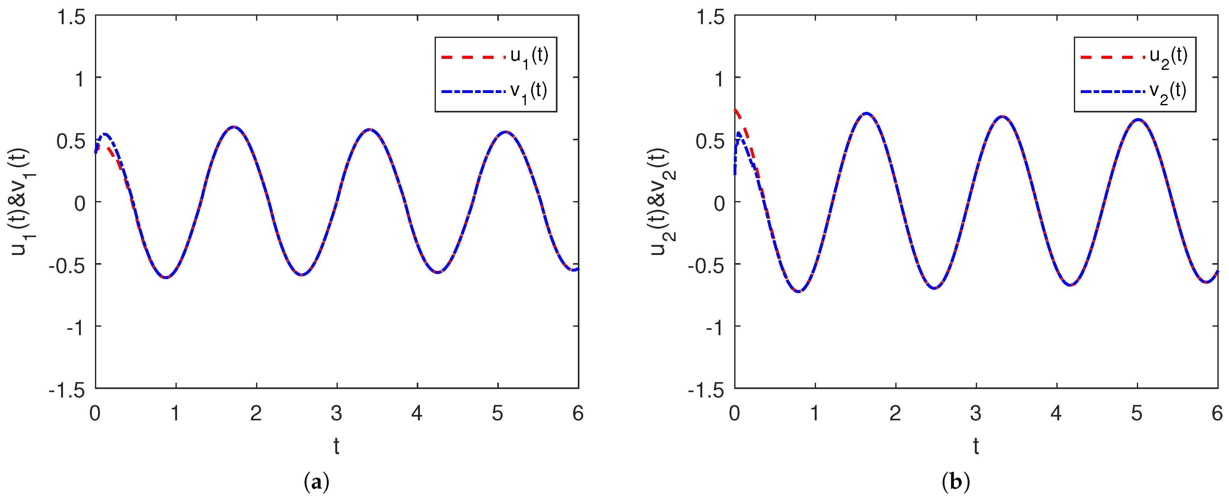
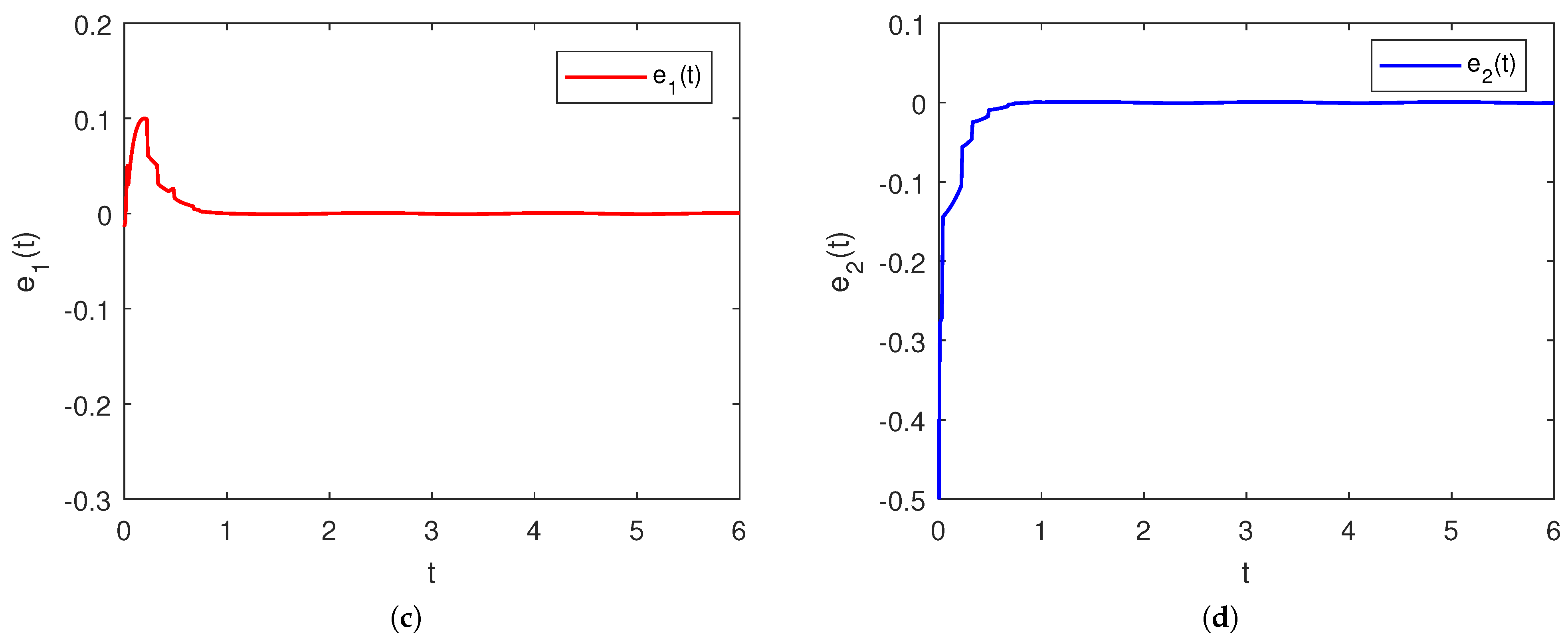
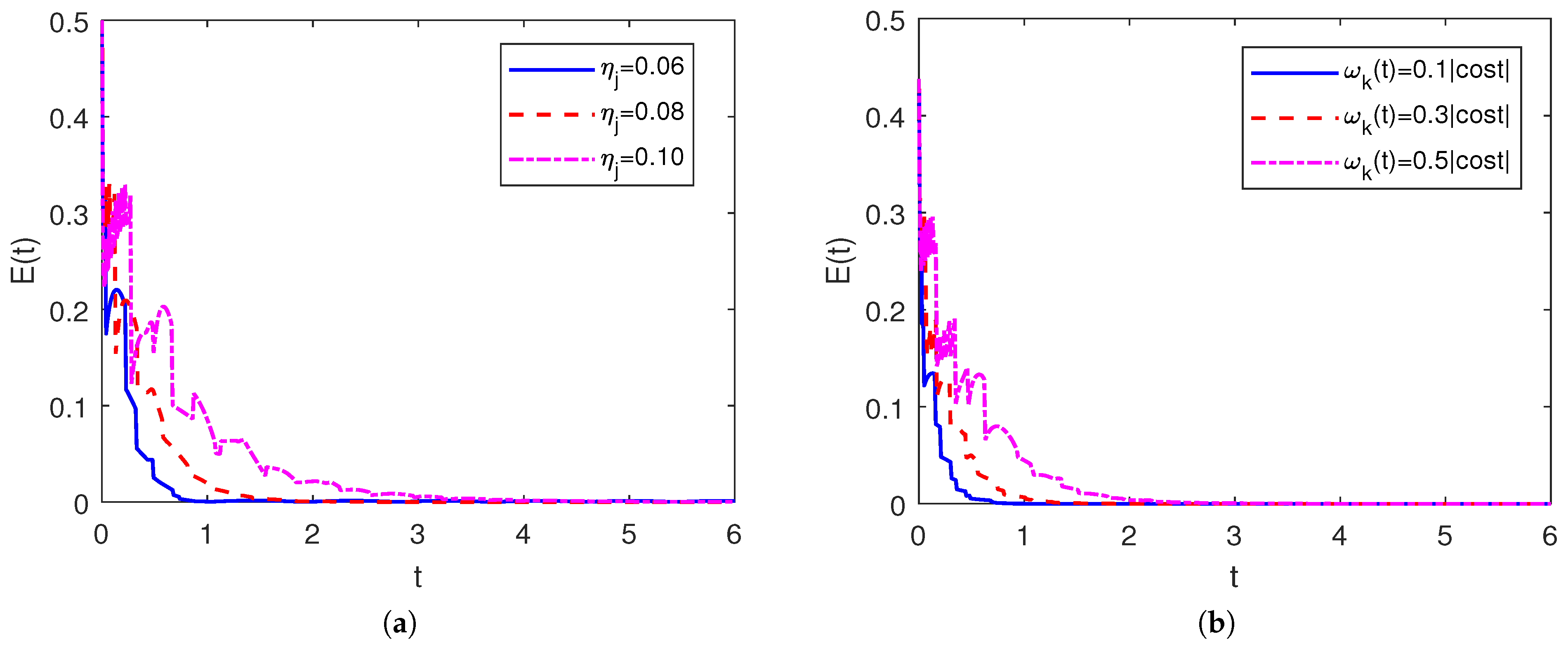
4. Illustrative Experiments

This section presents simulation experiments to verify the applicability of Theorems and the utilized controllers.
Example 1. Take a two-dimensional uncertain fractional-order memristive network as the master system.
D t ϱ 0 c u 1 ( t ) = ( b 1 + Δ b 1 ( t ) ) u 1 ( t ) + j = 1 2 c 1 j ( u j ( t ) ) tan h ( u j ( t ) ) + j = 1 2 d 1 j ( u j ( t η j ) ) × tan h ( u j ( t η j ) ) + I 1 ( t ) , D t ϱ 0 c u 2 ( t ) = ( b 2 + Δ b 2 ( t ) ) u 2 ( t ) + j = 1 2 c 2 j ( u j ( t ) ) tan h ( u j ( t ) ) + j = 1 2 d 2 j ( u j ( t η j ) ) × tan h ( u j ( t η j ) ) + I 2 ( t ) ,
where
c 11 ( u 1 ) = 1.2 , | u 1 ( t ) | < 1 , 1.0 , | u 1 ( t ) | > 1 ,   c 12 ( u 2 ) = 0.2 , | u 2 ( t ) | < 1 , 0.3 , | u 2 ( t ) | > 1 ,
c 21 ( u 1 ) = 1.5 , | u 1 ( t ) | < 1 , 1.0 , | u 1 ( t ) | > 1 ,   c 22 ( u 2 ) = 1.8 , | u 2 ( t ) | < 1 , 1.5 , | u 2 ( t ) | > 1 ,
d 11 ( u 1 ) = 2.0 , | u 1 ( t ) | < 1 , 1.0 , | u 1 ( t ) | > 1 ,   d 12 ( u 2 ) = 0.5 , | u 2 ( t ) | < 1 , 0.4 , | u 2 ( t ) | > 1 ,
d 21 ( u 1 ) = 1.5 , | u 1 ( t ) | < 1 , 1.0 , | u 1 ( t ) | > 1 ,   d 22 ( u 2 ) = 2.0 , | u 2 ( t ) | < 1 , 1.5 , | u 2 ( t ) | > 1 ,
ϱ = 0.95 , η 1 = 0.05 , η 2 = 0.05 , b 1 = 1 , b 2 = 1 , Δ b 1 ( t ) = 0.1 sin t , Δ b 2 ( t ) = 0.2 sin t , I 1 ( t ) = I 2 ( t ) = 0 .
Based on master system (45), the proportionate slave system is described by
D t ϱ 0 c v 1 ( t ) = ( b 1 + Δ b 1 ( t ) ) v 1 ( t ) + j = 1 2 c 1 j ( v j ( t ) ) tan h ( v j ( t ) ) + j = 1 2 d 1 j ( v j ( t η j ) ) × tan h ( v j ( t η j ) ) + I 1 ( t ) + ϖ 1 ( t ) + U 1 ( t ) , D t ϱ 0 c v 2 ( t ) = ( b 2 + Δ b 2 ( t ) ) v 2 ( t ) + j = 1 2 c 2 j ( v j ( t ) ) tan h ( v j ( t ) ) + j = 1 2 d 2 j ( v j ( t η j ) ) × tan h ( v j ( t η j ) ) + I 2 ( t ) + ϖ 2 ( t ) + U 2 ( t ) ,
where
c 11 ( v 1 ) = 1.2 , | v 1 ( t ) | < 1 , 1.0 , | v 1 ( t ) | > 1 ,   c 12 ( v 2 ) = 0.2 , | v 2 ( t ) | < 1 , 0.3 , | v 2 ( t ) | > 1 ,
c 21 ( v 1 ) = 1.5 , | v 1 ( t ) | < 1 , 1.0 , | v 1 ( t ) | > 1 ,   c 22 ( v 2 ) = 1.8 , | v 2 ( t ) | < 1 , 1.5 , | v 2 ( t ) | > 1 ,
d 11 ( v 1 ) = 2.0 , | v 1 ( t ) | < 1 , 1.0 , | v 1 ( t ) | > 1 ,   d 12 ( v 2 ) = 0.5 , | v 2 ( t ) | < 1 , 0.4 , | v 2 ( t ) | > 1 ,
d 21 ( v 1 ) = 1.5 , | v 1 ( t ) | < 1 , 1.0 , | v 1 ( t ) | > 1 ,   d 22 ( v 2 ) = 2.0 , | v 2 ( t ) | < 1 , 1.5 , | v 2 ( t ) | > 1 ,
ϖ 1 ( t ) = 0.1 | cos t | , ϖ 2 ( t ) = 0.2 | cos t | , and other network parameters can be acquired from system (45). For the activation functions ϕ j = ψ j = tan h ( · ) , one can obtain ϕ ¯ j = ψ ¯ j = 1 and L j ϕ = L j ψ = 1 that satisfies Assumptions 1–2. Selecting control strengths ρ 1 = ρ 2 = 3 , β 1 = 5.6 , β 2 = 8.4 , and simple calculations indicate that ϵ 1 = b 1 + ρ 1 ϑ 1 j = 1 2 c ¯ j 1 ϕ ¯ 1 = 1.2 , ϵ 2 = b 2 + ρ 2 ϑ 2 j = 1 2 c ¯ j 2 ϕ ¯ 2 = 1.7 . Hence, one can find that the restriction requirements of Theorem 1 are fulfilled.
The starting conditions of memristive systems (45) and (46) are generated stochastically in [ 0 , 1 ] . To achieve the synchronization objective, control scheme (16) is utilized. As shown in Figure 1a,b, the red curve and blue curve characterize the time evolution of state variables in the master system and slave system, respectively. Figure 1c,d show that the error system converges within a finite time, indicating the correctness of theoretical analysis in Theorem 1. Hence, memristive neural networks (45) and (46) can achieve finite-time synchronization with appropriate control parameters. In addition, the setting time T 1 * = 0.7653 is evaluated by Theorem 1. To explore the effect of control strength ρ k on synchronization efficiency, we increase control strength ρ k = 3 to ρ k = 3.5 so that the conditions in Theorem 1 still hold. As one can see in Figure 2, finite-time synchronization purposes can still be achieved, and the efficiency and speed of synchronization are faster than before. This means increasing control gain is beneficial for accelerating network synchronization.
In the previous experiments, we have verified that the memristive systems (45) and (46) can achieve Mittag-Leffler synchronization when the system parameters satisfy the constraints of Theorem 1. To study the relationship between system parameters and the synchronization efficiency of neural networks, we focus on two types of parameters including time delays and external perturbations. To facilitate the observation of the synchronization process changes, we first define total synchronization errors as E ( t ) = i = 1 n | e i ( t ) | . First, we set the initial time delay to 0.06, and it gradually increases to 0.10 with a step size of 0.02. The experimental results are given in Figure 3a, which shows that the time required for the network to reach synchronization increases gradually as the delays become larger. This indicates that large time delays have a greater impact on the stability of the systems. In addition, we set the perturbations as 0.1 | c o s t | , 0.3 | c o s t | , and 0.5 | c o s t | , respectively. The experimental results are shown in Figure 3b. As the amplitude of the perturbations increases, the more time it takes for the network to achieve synchronization. This indicates that the larger the amplitude of the perturbations, the greater the effect on the stability of the systems.
Example 2. Contemplate a three-dimensional uncertain Caputo fractional memristive network as the drive system, which can be given by
D t ϱ 0 c u 1 ( t ) = ( b 1 + Δ b 1 ( t ) ) u 1 ( t ) + j = 1 3 c 1 j ( u j ) tan h ( u j ( t ) ) + j = 1 3 d 1 j ( u j ( t η j ) ) × tan h ( u j ( t η j ) ) + I 1 ( t ) , D t ϱ 0 c u 2 ( t ) = ( b 2 + Δ b 2 ( t ) ) u 2 ( t ) + j = 1 3 c 2 j ( u j ) tan h ( u j ( t ) ) + j = 1 3 d 2 j ( u j ( t η j ) ) × tan h ( u j ( t η j ) ) + I 2 ( t ) , D t ϱ 0 c u 3 ( t ) = ( b 3 + Δ b 3 ( t ) ) u 3 ( t ) + j = 1 3 c 3 j ( u j ) tan h ( u j ( t ) ) + j = 1 3 d 3 j ( u j ( t η j ) ) × tan h ( u j ( t η j ) ) + I 3 ( t ) ,
where
c 11 ( u 1 ) = 3.2 , | u 1 ( t ) | < 1 , 3.1 , | u 1 ( t ) | > 1 ,   c 12 ( u 2 ) = 2.0 , | u 2 ( t ) | < 1 , 1.1 , | u 2 ( t ) | > 1 ,
c 13 ( u 3 ) = 3.1 , | u 3 ( t ) | < 1 , 4.1 , | u 3 ( t ) | > 1 ,   c 21 ( u 1 ) = 1.0 , | u 1 ( t ) | < 1 , 0.9 , | u 1 ( t ) | > 1 ,
c 22 ( u 2 ) = 2.0 , | u 2 ( t ) | < 1 , 1.9 + π 4 , | u 2 ( t ) | > 1 ,   c 23 ( u 3 ) = 0.9 , | u 3 ( t ) | < 1 , 5.0 , | u 3 ( t ) | > 1 ,
c 31 ( u 1 ) = 3.5 , | u 1 ( t ) | < 1 , 6.1 , | u 1 ( t ) | > 1 ,   c 32 ( u 2 ) = 1.2 , | u 2 ( t ) | < 1 , 1.6 , | u 2 ( t ) | > 1 ,
c 33 ( u 3 ) = 2.0 , | u 3 ( t ) | < 1 , 1.1 , | u 3 ( t ) | > 1 ,   d 11 ( u 1 ) = 2.2 , | u 1 ( t ) | < 1 , 2.2 , | u 1 ( t ) | > 1 ,
d 12 ( u 2 ) = 0.15 , | u 2 ( t ) | < 1 , 0.23 , | u 2 ( t ) | > 1 ,   d 13 ( u 3 ) = 0.85 , | u 3 ( t ) | < 1 , 0.9 , | u 3 ( t ) | > 1 ,
d 21 ( u 1 ) = 1.8 , | u 1 ( t ) | < 1 , 1.4 , | u 1 ( t ) | > 1 ,   d 22 ( u 2 ) = 1.5 , | u 2 ( t ) | < 1 , 1.6 , | u 2 ( t ) | > 1 ,
d 23 ( u 3 ) = 0.2 , | u 3 ( t ) | < 1 , 0.3 , | u 3 ( t ) | > 1 ,   d 31 ( u 1 ) = 2.3 , | u 1 ( t ) | < 1 , 2.1 , | u 1 ( t ) | > 1 ,
d 32 ( u 2 ) = 2.9 , | u 2 ( t ) | < 1 , 2.0 , | u 2 ( t ) | > 1 ,   d 33 ( u 3 ) = 1.1 , | u 3 ( t ) | < 1 , 1.3 , | u 3 ( t ) | > 1 ,
ϱ = 0.98 , η 1 = 0.2 , η 2 = 0.3 , η 3 = 0.4 b 1 = b 2 = b 3 = 1 , Δ b 1 ( t ) = Δ b 2 ( t ) = 0.1 sin t , Δ b 3 ( t ) = 0.2 sin t , I 1 ( t ) = I 2 ( t ) = I 3 ( t ) = 0 .
According to master neural networks (47), the proportionate slave system consisting of neural networks can be expressed by
D t ϱ 0 c v 1 ( t ) = ( b 1 + Δ b 1 ( t ) ) v 1 ( t ) + j = 1 3 c 1 j ( v j ) tan h ( v j ( t ) ) + j = 1 3 d 1 j ( v j ( t η j ) ) × tan h ( v j ( t η j ) ) + I 1 ( t ) + ϖ 1 ( t ) + U 1 ( t ) , D t ϱ 0 c v 2 ( t ) = ( b 2 + Δ b 2 ( t ) ) v 2 ( t ) + j = 1 3 c 2 j ( v j ) tan h ( v j ( t ) ) + j = 1 3 d 2 j ( v j ( t η j ) ) × tan h ( v j ( t η j ) ) + I 2 ( t ) + ϖ 2 ( t ) + U 2 ( t ) , D t ϱ 0 c v 3 ( t ) = ( b 3 + Δ b 3 ( t ) ) v 3 ( t ) + j = 1 3 c 3 j ( v j ) tan h ( v j ( t ) ) + j = 1 3 d 3 j ( v j ( t η j ) ) × tan h ( v j ( t η j ) ) + I 3 ( t ) + ϖ 3 ( t ) + U 3 ( t ) ,
where
c 11 ( v 1 ) = 3.2 , | v 1 ( t ) | < 1 , 3.1 , | v 1 ( t ) | > 1 ,   c 12 ( v 2 ) = 2.0 , | v 2 ( t ) | < 1 , 1.1 , | v 2 ( t ) | > 1 ,
c 13 ( v 3 ) = 3.1 , | v 3 ( t ) | < 1 , 4.1 , | v 3 ( t ) | > 1 ,   c 21 ( v 1 ) = 1.0 , | v 1 ( t ) | < 1 , 0.9 , | v 1 ( t ) | > 1 ,
c 22 ( v 2 ) = 2.0 , | v 2 ( t ) | < 1 , 1.9 + π 4 , | v 2 ( t ) | > 1 ,   c 23 ( v 3 ) = 0.9 , | v 3 ( t ) | < 1 , 5.0 , | v 3 ( t ) | > 1 ,
c 31 ( v 1 ) = 3.5 , | v 1 ( t ) | < 1 , 6.1 , | v 1 ( t ) | > 1 ,   c 32 ( v 2 ) = 1.2 , | v 2 ( t ) | < 1 , 1.6 , | v 2 ( t ) | > 1 ,
c 33 ( v 3 ) = 2.0 , | v 3 ( t ) | < 1 , 1.1 , | v 3 ( t ) | > 1 ,   d 11 ( v 1 ) = 2.2 , | v 1 ( t ) | < 1 , 2.2 , | v 1 ( t ) | > 1 ,
d 12 ( v 2 ) = 0.15 , | v 2 ( t ) | < 1 , 0.23 , | v 2 ( t ) | > 1 ,   d 13 ( v 3 ) = 0.85 , | v 3 ( t ) | < 1 , 0.9 , | v 3 ( t ) | > 1 ,
d 21 ( v 1 ) = 1.8 , | v 1 ( t ) | < 1 , 1.4 , | v 1 ( t ) | > 1 ,   d 22 ( v 2 ) = 1.5 , | v 2 ( t ) | < 1 , 1.6 , | v 2 ( t ) | > 1 ,
d 23 ( v 3 ) = 0.2 , | v 3 ( t ) | < 1 , 0.3 , | v 3 ( t ) | > 1 ,   d 31 ( v 1 ) = 2.3 , | v 1 ( t ) | < 1 , 2.1 , | v 1 ( t ) | > 1 ,
d 32 ( v 2 ) = 3 , | v 2 ( t ) | < 1 , 2 , | v 2 ( t ) | > 1 ,   d 33 ( v 3 ) = 1.1 , | v 3 ( t ) | < 1 , 1.3 , | v 3 ( t ) | > 1 ,
ϖ 1 ( t ) = 0.1 | sin t + cos t | , ϖ 2 ( t ) = ϖ 3 ( t ) = 0.2 | sin t cos t | , and other system parameters are the same as system (47).
Selecting control strengths ρ 1 = 10 , ρ 2 = 8 , ρ 3 = 10.2 , β 1 = 10 , β 2 = 13 , β 3 = 19 , and simple calculations indicate that ε 1 = b 1 + ρ 1 ϑ 1 1 2 j = 1 3 ( c ¯ 1 j ϕ ¯ j + c ¯ j 1 ϕ ¯ 1 ) = 1.1 , ε 2 = b 2 + ρ 2 ϑ 2 1 2 j = 1 3 ( c ¯ 2 j ϕ ¯ j + c ¯ j 2 ϕ ¯ 2 ) = 1.415 , ε 3 = b 3 + ρ 3 ϑ 3 1 2 j = 1 3 ( c ¯ 3 j ϕ ¯ j + c ¯ j 3 ϕ ¯ 3 ) = 0.6 . Hence, one can find that the restriction requirements of Theorem 2 are satisfied.
The starting conditions of memristor-based systems (47) and (48) are randomly selected in [ 5 , 5 ] . To achieve the synchronization objective, feedback control schemes (37) are applied. As seen in Figure 4a–c, two different curves, u i ( t ) and v i ( t ) , represent the time evolution of state variables in the master and slave neural networks. Furthermore, Figure 4d–f display that the error neural network converges within a finite time, implying the validity of theoretical results in Theorem 2. In addition, the setting time T 2 * = 0.5241 is evaluated by Theorem 2. Consequently, memristor-based network systems (47) and (48) can achieve finite-time synchronization under the control methods (37).

5. Conclusions

This study focuses on the Mittag-Leffler synchronization in finite time for generalized FMMNNs. In particular, uncertainties, time-varying perturbations, and transmission delays are introduced into the system to model more realistic fractional networks. Utilizing two simple feedback controllers involving sign functions, new synchronization criteria concerning the FMMNN are obtained, which depend on the control strength, perturbation boundaries, uncertainty boundaries, and system parameters. Most works have been performed to address the influence of different delays on the stability of the error network, usually using the comparison principle. This study attempts to overcome this difficulty directly using inequality techniques rather than comparison principles. Finally, experiment results demonstrate the effectiveness of the controller and obtained conclusions. This study removes the constraint that the activation function has a zero function value at switching jumps. Based on event-triggered intermittent feedback control, we will continue to deliberate the finite-time synchronization challenge of high-order topology memristive neural networks in the future.

Author Contributions

Conceptualization, K.S., H.F. and H.W.; Methodology, Y.L., K.S. and H.W.; Software, X.C., Y.L., H.F. and Y.W.; Writing—original draft, H.F., X.C., Y.W. and Y.L.; Writing—review and editing, X.C., K.S. and H.W. All authors have read and agreed to the published version of the manuscript.

Funding

The first author was partially supported by the Open Foundation of Engineering Research Center of Big Data Application in Private Health Medicine, Fujian Province University under grant (MKF202201). The third author was partially supported by the Sichuan Science and Technology Program under grant (21YYJC0469), and the Key R&D Projects of Sichuan Provincial Department of Science and Technology under grant (2023YFG0287). The fifth author was partially supported by the Sichuan Education Development Research Center of West China Normal University Funded Project under grant (CJF23042), and the Sichuan Teacher Education Research Center Funded Project under grant (TER2023-017). The sixth author was partially supported by the Ministry of Education’s Industry–University Cooperation Collaborative Education Project under grant (231102311285117), the Introducing Talent Projects of Putian University (Seedling Fund) under grant (2019110), and the Natural Science Foundation of Fujian Province under grant (2023J011015), and the APC was funded by (2023J011015).

Data Availability Statement

Data is contained within the article.

Conflicts of Interest

The authors declare no conflicts of interest.

References

  1. Tang, Z.; Xuan, D.L.; Park, J.H.; Wang, Y.; Feng, J.W. Impulsive effects based distributed synchronization of heterogeneous coupled neural networks. IEEE Trans. Netw. Sci. Eng. 2021, 8, 498–510. [Google Scholar] [CrossRef]
  2. Fan, H.G.; Chen, X.J.; Shi, K.B.; Wen, H. Distributed delayed impulsive control for μ-synchronization of multi-link structure networks with bounded uncertainties and time-varying delays of unmeasured bounds: A novel Halanay impulsive inequality approach. Chaos Solitons Fractals 2024, 186, 115226. [Google Scholar] [CrossRef]
  3. Zhong, Q.S.; Han, S.; Shi, K.B.; Zhong, S.M.; Kwon, O.-M. Co-design of adaptive memory event-triggered mechanism and aperiodic intermittent controller for nonlinear networked control systems. IEEE Trans. Circuits Syst.-Express Briefs 2022, 69, 4979–4983. [Google Scholar] [CrossRef]
  4. Cai, J.Y.; Yi, C.B.; Wu, Y.; Liu, D.Q.; Zhong, D.G. Leader-following consensus of nonlinear singular switched multi-agent systems via sliding mode control. Asian J. Control 2024, 26, 1–14. [Google Scholar] [CrossRef]
  5. Zhou, C.; Wang, C.H.; Yao, W.; Lin, H.R. Observer-based synchronization of memristive neural networks under dos attacks and actuator saturation and its application to image encryption. Appl. Math. Comput. 2022, 425, 127080. [Google Scholar] [CrossRef]
  6. Cheng, J.; Lin, A.; Cao, J.D.; Qiu, J.L.; Qi, W.H. Protocol-based fault detection for discrete-time memristive neural networks with effect. Inf. Sci. 2022, 615, 118–135. [Google Scholar] [CrossRef]
  7. Tang, C.; Li, X.Q.; Wang, Q. Mean-field stochastic linear quadratic optimal control for jump-diffusion systems with hybrid disturbances. Symmetry 2024, 16, 642. [Google Scholar] [CrossRef]
  8. Fan, H.G.; Rao, Y.; Shi, K.B.; Wen, H. Time-varying function matrix projection synchronization of Caputo fractional-order uncertain memristive neural networks with multiple delays via mixed open loop feedback control and impulsive control. Fractal Fract. 2024, 8, 301. [Google Scholar] [CrossRef]
  9. Shi, K.B.; Cai, X.; She, K.; Wen, S.P.; Zhong, S.M.; Park, P.; Kwon, O.-M. Stability analysis and security-based event-triggered mechanism design for T-S fuzzy NCS with traffic congestion via DoS attack and its application. IEEE Trans. Fuzzy Syst. 2023, 31, 3639–3651. [Google Scholar] [CrossRef]
  10. Kong, F.C.; Zhu, Q.X.; Huang, T.W. New fixed-time stability lemmas and applications to the discontinuous fuzzy inertial neural networks. IEEE Trans. Fuzzy Syst. 2021, 29, 3711–3722. [Google Scholar] [CrossRef]
  11. Ding, K.; Zhu, Q.X. A note on sampled-data synchronization of memristor networks subject to actuator failures and two different activations. IEEE Trans. Circuits Syst. II Express Briefs 2021, 68, 2097–2101. [Google Scholar] [CrossRef]
  12. Adhikari, S.P.; Yang, C.; Kim, H.; Chua, L.O. Memristor bridge synapse-based neural network and its learning. IEEE Trans. Neural Netw. Learn. Syst. 2012, 23, 1426–1435. [Google Scholar] [CrossRef]
  13. Dou, H.; Shen, F.; Zhao, J.; Mu, X.Y. Understanding neural network through neuron level visualization. Neural Netw. 2023, 168, 484–495. [Google Scholar] [CrossRef] [PubMed]
  14. Wang, X.; Park, J.H.; Zhong, S.M.; Yang, H.L. A switched operation approach to sampled-data control stabilization of fuzzy memristive neural networks with time-varying delay. IEEE Trans. Neural Netw. Learn. Syst. 2020, 31, 891–900. [Google Scholar] [CrossRef] [PubMed]
  15. Alsaedi, A.; Cao, J.D.; Ahmad, B.; Alshehri, A.; Tan, X.G. Synchronization of master-slave memristive neural networks via fuzzy output-based adaptive strategy. Chaos Solitons Fractals 2022, 158, 112095. [Google Scholar] [CrossRef]
  16. Hua, W.T.; Wang, Y.T.; Liu, C.Y. New method for global exponential synchronization of multi-link memristive neural networks with three kinds of time-varying delays. Appl. Math. Comput. 2024, 471, 128593. [Google Scholar] [CrossRef]
  17. Bao, H.B.; Park, J.H.; Cao, J.D. Exponential synchronization of coupled stochastic memristor-based neural networks with time-varying probabilistic delay coupling and impulsive delay. IEEE Trans. Neural Netw. Learn. Syst. 2016, 27, 190–201. [Google Scholar] [CrossRef]
  18. Li, X.F.; Zhang, W.B.; Fang, J.A.; Li, H.Y. Finite-time synchronization of memristive neural networks with discontinuous activation functions and mixed time-varying delays. Neurocomputing 2019, 340, 99–109. [Google Scholar] [CrossRef]
  19. Yu, T.H.; Cao, J.D.; Rutkowski, L.; Luo, Y.P. Finite-time synchronization of complex-valued memristive-based neural networks via hybrid controls. IEEE Trans. Neural Netw. Learn. Syst. 2022, 33, 3938–3947. [Google Scholar] [CrossRef]
  20. Fu, Q.H.; Zhong, S.M.; Jiang, W.B.; Xie, W.Q. Projective synchronization of fuzzy memristive neural networks with pinning impulsive control. J. Frankl. Inst. 2020, 357, 10387–10409. [Google Scholar] [CrossRef]
  21. Podlubny, I. Fractional Differential Equations; Academic Press: New York, NY, USA, 1999. [Google Scholar]
  22. Chen, L.P.; Cao, J.D.; Wu, R.C.; Machado, J.A.T.; Lopes, A.M.; Yang, H.J. Stability and synchronization of fractional-order memristive neural networks with multiple delays. Neural Netw. 2017, 94, 76–85. [Google Scholar] [CrossRef]
  23. Gu, Y.J.; Wang, H.; Yu, Y.G. Synchronization for commensurate Riemann-Liouville fractional-order memristor-based neural networks with unknown parameters. J. Frankl. Inst. 2020, 357, 8870–8898. [Google Scholar] [CrossRef]
  24. Chen, J.J.; Zeng, Z.G.; Jiang, P. Global Mittag-Leffler stability and synchronization of memristor-based fractional-order neural networks. Neural Netw. 2014, 51, 1–8. [Google Scholar] [CrossRef]
  25. Bao, H.B.; Cao, J.D. Projective synchronization of fractional-order memristor-based neural networks. Neural Netw. 2015, 63, 1–9. [Google Scholar] [CrossRef] [PubMed]
  26. Zhang, L.Z.; Yang, Y.Q.; Wang, F. Projective synchronization of fractional-order memristor-based neural networks with switching jumps mismatch. Phys. A 2017, 471, 402–415. [Google Scholar] [CrossRef]
  27. Velmurugan, G.; Rakkiyappan, R. Hybrid projective synchronization of fractional-order memristor-based neural networks with time delays. Nonlinear Dyn. 2016, 83, 419–432. [Google Scholar] [CrossRef]
  28. Li, X.M.; Liu, X.G.; Wang, F.X. Anti-synchronization of fractional-order complex-valued neural networks with a leakage delay and time-varying delays. Chaos Solitons Fractals 2023, 174, 113754. [Google Scholar] [CrossRef]
  29. Peng, L.B.; Li, X.F.; Bi, D.J.; Xie, X.; Xie, Y.L. Pinning multisynchronization of delayed fractional-order memristor-based neural networks with nonlinear coupling and almost-periodic perturbations. Neural Netw. 2021, 144, 372–383. [Google Scholar] [CrossRef]
  30. Gu, Y.J.; Yu, Y.G.; Wang, H. Projective synchronization for fractional-order memristor-based neural networks with time delays. Neural Comput. Appl. 2019, 31, 6039–6054. [Google Scholar] [CrossRef]
  31. Song, S.; Song, X.N.; Balsera, I.T. Mixed H and passive projective synchronization for fractional-order memristor-based neural networks with time delays via adaptive sliding mode control. Neural Process. Lett. 2018, 47, 443–462. [Google Scholar] [CrossRef]
  32. Mao, X.Y.; Wang, X.M.; Lu, Y.X.; Qin, H.Y. Synchronizations control of fractional-order multidimension-valued memristive neural networks with delays. Neurocomputing 2024, 563, 126942. [Google Scholar] [CrossRef]
  33. Si, X.; Wang, Z.; Fan, Y. Quantized control for finite-time synchronization of delayed fractional-order memristive neural networks: The Gronwall inequality approach. Expert Syst. Appl. 2023, 215, 119310. [Google Scholar] [CrossRef]
  34. Peng, X.; Wu, H.Q.; Song, K.; Shi, J.X. Global synchronization in finite time for fractional-order neural networks with discontinuous activations and time delays. Neural Netw. 2017, 94, 46–54. [Google Scholar] [CrossRef] [PubMed]
  35. Mao, K.; Liu, X.Y.; Cao, J.D.; Hu, Y.F. Finite-time bipartite synchronization of coupled neural networks with uncertain parameters. Phys. A 2022, 585, 126431. [Google Scholar] [CrossRef]
  36. Yang, X.J.; Li, C.D.; Huang, T.W.; Song, Q.K.; Huang, J.J. Synchronization of fractional-order memristor-based complex-valued neural networks with uncertain parameters and time delays. Chaos Solitons Fractals 2018, 110, 105–123. [Google Scholar] [CrossRef]
  37. Yu, Y.G.; Zhang, S. Robust synchronization of memristor-based fractional-order Hopfield neural networks with parameter uncertainties. Neural Comput. Appl. 2019, 31, 3533–3542. [Google Scholar]
  38. Yao, W.; Wang, C.H.; Sun, Y.C.; Gong, S.Q.; Lin, H.R. Event-triggered control for robust exponential synchronization of inertial memristive neural networks under parameter disturbance. Neural Netw. 2023, 164, 67–80. [Google Scholar] [CrossRef] [PubMed]
  39. Yan, H.Y.; Qiao, Y.H.; Ren, Z.H.; Duan, L.J.; Miao, J. Master-slave synchronization of fractional-order memristive MAM neural networks with parameter disturbances and mixed delays. Commun. Nonlinear Sci. Numer. Simul. 2023, 120, 107152. [Google Scholar] [CrossRef]
  40. Liu, P.; Zeng, Z.; Wang, J. Asymptotic and finite-time cluster synchronization of coupled fractional-order neural networks with time delay. IEEE Trans. Neural Netw. Learn. Syst. 2020, 31, 4956–4967. [Google Scholar] [CrossRef]
  41. Abdeljawad, T.; SThabet, T.; Kedim, I.; Ayari, M.I.; Khan, A. A higher-order extension of Atangana–Baleanu fractional operators with respect to another function and a Gronwall-type inequality. Bound. Value Probl. 2023, 2023, 49. [Google Scholar] [CrossRef]
  42. Alzahrani, A.B.; Saadeh, R.; Abdoon, M.A.; Elbadri, M.; Berir, M.; Qazza, A. Effective methods for numerical analysis of the simplest chaotic circuit model with Atangana–Baleanu Caputo fractional derivative. J. Eng. Math. 2024, 144, 9. [Google Scholar] [CrossRef]
  43. Yasmin, H. Application of aboodh homotopy perturbation transform method for fractional-order convection–reaction-diffusion equation within Caputo and Atangana–Baleanu operators. Symmetry 2023, 15, 453. [Google Scholar] [CrossRef]
  44. Zhang, S.; Yu, Y.G.; Wang, H. Mittag-Leffler stability of fractional-order Hopfield neural networks. Nonlinear Anal. Hybrid Syst. 2015, 16, 104–121. [Google Scholar] [CrossRef]
  45. Li, H.L.; Jiang, Y.L.; Wang, Z.L.; Zhang, L.; Teng, Z.D. Global Mittag-Leffler stability of coupled system of fractional-order differential equations on network. Appl. Math. Comput. 2015, 270, 269–277. [Google Scholar] [CrossRef]
  46. Arslan, E.; Narayanan, G.; Syed Ali, M.; Arik, S.; Saroha, S. Controller design for finite-time and fixed-time stabilization of fractional-order memristive complex-valued BAM neural networks with uncertain parameters and time-varying delays. Neural Netw. 2020, 130, 60–74. [Google Scholar] [CrossRef]
Figure 1. The curves of state vectors and error vectors for uncertain FMMNNs (45) and (46) under control schemes (16) with control gain ρ k = 3 in Example 1. (a) State vectors u 1 ( t ) and v 1 ( t ) ; (b) state vectors u 2 ( t ) and v 2 ( t ) ; (c) synchronization error e 1 ( t ) ; (d) synchronization error e 2 ( t ) .
Fractalfract 08 00422 g001aFractalfract 08 00422 g001b
Figure 2. The curves of state vectors and error vectors for uncertain FMMNNs (45) and (46) under control schemes (16) with control gain ρ k = 3.5 in Example 1. (a) State vectors u 1 ( t ) and v 1 ( t ) ; (b) state vectors u 2 ( t ) and v 2 ( t ) ; (c) synchronization error e 1 ( t ) ; (d) synchronization error e 2 ( t ) .
Fractalfract 08 00422 g002
Figure 3. The curves of total synchronization errors for uncertain FMMNNs (45) and (46) under control schemes (16) with different parameters in Example 1. (a) Time evolution of time delays η j and total synchronization errors E ( t ) ; (b) time evolution of perturbations ω k and total synchronization errors E ( t ) .
Fractalfract 08 00422 g003
Figure 4. The curves of state vectors and error vectors for uncertain FMMNNs (47) and (48) under control schemes (37) in Example 2. (a) State vectors u 1 ( t ) and v 1 ( t ) ; (b) state vectors u 2 ( t ) and v 2 ( t ) ; (c) state vectors u 3 ( t ) and v 3 ( t ) ; (d) synchronization error e 1 ( t ) ; (e) synchronization error e 2 ( t ) ; (f) synchronization error e 3 ( t ) .
Fractalfract 08 00422 g004
Disclaimer/Publisher’s Note: The statements, opinions and data contained in all publications are solely those of the individual author(s) and contributor(s) and not of MDPI and/or the editor(s). MDPI and/or the editor(s) disclaim responsibility for any injury to people or property resulting from any ideas, methods, instructions or products referred to in the content.

