A Novel Semi-Analytical Scheme to Deal with Fractional Partial Differential Equations (PDEs) of Variable-Order

Abstract

This article introduces a new numerical algorithm dedicated to solving the most general form of variable-order fractional partial differential models. Both the time and spatial order of derivatives are considered as non-constant values. A combination of the shifted Chebyshev polynomials is used to approximate the solution of such equations. The coefficients of this combination are considered a function of time, and they are obtained using the collocation method. The theoretical aspects of the method are investigated, and then by solving some problems, the efficiency of the method is presented.

1. Introduction

Fractional-order integration and differentiation constitute the essence of fractional calculus. From the middle of the previous century, fractional calculus has had a very important effect in many different areas. One may find a few such areas in the book that is written by Diethelm [1]. In fractional calculus, the order of the integration or differentiation operator is usually indicated by a constant, positive, and real number, e.g., $\alpha$.

In 1993, Ross and Samko [2] presented the concept of the fractional derivative and integration operators with variable-orders. The order of their operators was a function of t, i.e., $\alpha \left(t\right)$. In such operations, the order of operators can vary from point to point. In fact, they extended the constant-order fractional derivative to a variable-order one. Their work was followed by some researchers, most of whom worked on the theoretical aspect of the subject. Samko [3] presented a thorough investigation into fractional integration and differentiation with the variable-order. Further, Sun et al. [4] performed a comparative analysis between constant-order and variable-order fractional models. There is a suitable review on the variable-order of fractional calculus in [5]. Also, one may find good acknowledgment of fractional-order calculus of variations in [6]. Chechkin et al. [7] obtained a time-fractional equation along with a spatially varying fractional order of the time differentiation by starting from a continuous case time random walk approach with a space-dependent waiting-time probability density function. Zheng et al. [8] investigated the solution regularity of a well-posed reaction–diffusion problem in its variable-order of the time-fractional case. They considered the kernel of the equation as the Mittag–Leffler one. It must be noted that in practical problems, a constant-order fractional derivative cannot adequately capture the variability of memory with respect to time. This limitation causes using the variable-order fractional operator. Guo and Zheng [9] recently investigated a diffusion equation with a variable-order time fractional and a Mittag–Leffler kernel.

Variable-order fractional partial differential equations (VOFPDEs) serve crucial roles in two important areas, namely, mechanics [10] and viscoelasticity [11]. Therefore, there have been some efforts to solve VOFPDEs by different methods, e.g., the operational matrix method [12], approximation by Jacobi [13] and Chebyshev polynomials [14], the spectral method [15], approximation by Legendre wavelets [16], the finite difference method [17], the reproducing kernel approach [18], and approximation by Bernstein polynomials [19].

The following general form for a space-time VOFPDE is considered in this article:

$${}_0{}^C\mathcal{D}_t^{\alpha \left(t\right)}v(x,t)+\sum _{i=1}^{n_1}{a}_i(x,t){}_0{}^C\mathcal{D}_t^{{\alpha }_i\left(t\right)}v(x,t)+\sum _{i=1}^{n_2}{b}_i(x,t){}_0{}^C\mathcal{D}_t^{{\beta }_i\left(t\right)}\left({}_a{}^C\mathcal{D}_x^{{\lambda }_i\left(x\right)}v(x,t)\right)=f(x,t),$$

(1)

and the initial/boundary conditions are considered as:

$$\begin{array}{c}\begin{array}{cccc}& v(x,0)=h_0\left(x\right),\hfill & \hfill {\displaystyle \frac{{\partial }^{i}v(x,0)}{\partial t^i}}=h_i\left(x\right),& i=1,2,\dots ,n-1,\mathrm{and}a\le x\le b,\hfill \\ & v(a,t)=g_0\left(t\right),\hfill & \hfill v(b,t)=g_1\left(t\right),& t\in [0,T],\hfill \end{array}\end{array}$$

(2)

where $\alpha \left(t\right)\in (n-1,n]$, ${\alpha }_i\left(t\right),{\beta }_i\left(t\right)\in (n-i-1,n-i]$, ${\lambda }_i\left(x\right)\in (0,1]$, or ${\lambda }_i\left(x\right)\in (1,2]$ and $n\in \mathbb{N}$. Also, $a_i(x,t)$, $b_i(x,t)$, $f(x,t)$, $h_0\left(x\right)$, $h_i\left(x\right)$, $g_0\left(t\right)$, and $g_1\left(t\right)$ are sufficiently smooth known functions.

To approximate the solution of Equation (1), a combination of shifted Chebyshev polynomials is employed, which makes a semi-analytical solution for it. The determination of the unknown coefficients in this combination is achieved through the collocation method.

2. Background Information

Within this section, we outline crucial definitions and notations that are fundamental for our subsequent discussions and analyses.

2.1. Fractional Derivative Operator

Here, we focus on the variable-order Caputo fractional derivative operator, whose order depends on time or space. The emphasis on variable-order fractional operators stems from their capacity to provide more accurate descriptions of numerous complex real-world problems. Some comparative investigations which characterize the importance of dealing with these types of operators rather than constant-order fractional derivatives were provided in [20,21,22]. Driven by the aforementioned considerations and motivations, the following definition for the variable-order Caputo fractional derivative can be stated.

Definition 1. 

The variable-order of Caputo fractional differentiation is expressed as:

$${}_a{}^C\mathcal{D}_x^{\alpha \left(x\right)}v(x,t)=\left\{\begin{array}{cc}{\displaystyle \frac{1}{\mathrm{\Gamma }(n-\alpha (x\left)\right)}}{\int }_a^x{(x-\tau )}^{n-\alpha \left(x\right)-1}{\displaystyle \frac{{\partial }^{n}v(\tau ,t)}{\partial {\tau }^n}}d\tau ,\hfill & \alpha \left(x\right)\in (n-1,n],\hfill \\ \hfill & \\ {\displaystyle \frac{{\partial }^{n}v(x,t)}{\partial x^n}},\hfill & \alpha \left(x\right)\equiv n,\hfill \end{array}\right.$$

wherein $\mathrm{\Gamma }(·)$ shows the well-known Gamma function.

Remark 1. 

By referring to Definition 1 and taking $v(x,t)={(x-a)}^{\ell }$, we have:

$${}_a{}^C\mathcal{D}_x^{\alpha \left(x\right)}{(x-a)}^{\ell }=\left\{\begin{array}{cc}{\displaystyle \frac{\mathrm{\Gamma }(\ell +1)}{\mathrm{\Gamma }(\ell -\alpha (x)+1)}}{(x-a)}^{\ell -\alpha \left(x\right)},\hfill & (\ell \in {\mathbb{N}}_0\wedge \ell \ge n)\vee (\ell \notin \mathbb{N}\wedge \ell >n-1),\hfill \\ 0,\hfill & \ell \in {\mathbb{N}}_0\wedge \ell <n,\hfill \end{array}\right.$$

where $n-1<\alpha \left(x\right)\le n$, and ${\mathbb{N}}_0=\mathbb{N}\cup \left\{0\right\}$.

2.2. Shifted Chebyshev Polynomials

Numerous studies in the past have extensively investigated the operational matrices of fractional-order derivatives, including the articles cited in [23,24]. In this present research, we adopt a similar approach to derive the Caputo derivative operator with variable-order using shifted Chebyshev polynomials. Therefore, the following special framework of weighted $L^2$-spaces is considered:

$$L_{\omega }^2\left(\mathrm{\Lambda }\right)=\left\{f:\mathrm{\Lambda }\to \mathbb{R}|{\int }_{\mathrm{\Lambda }}{\left|f\left(x\right)\right|}^2\omega \left(x\right)dx<\infty ,\mathrm{and}f\mathrm{is}\mathrm{measurable}\right\},$$

where weight function $\omega \left(x\right)$ shows a measurable positive, and $\mathrm{\Lambda }\subset \mathbb{R}$. Additionally, the relevant scalar product and norm functions are described as follows:

$${(f,g)}_{\omega }={\int }_{\mathrm{\Lambda }}f\left(x\right)g\left(x\right)\omega \left(x\right)dx,\mathrm{and}{\parallel f\parallel }_{\omega ,2}=\sqrt{{\int }_{\mathrm{\Lambda }}f{\left(x\right)}^2\omega \left(x\right)dx}.$$

It must be noted that the orthogonality between functions $f,g\in L_{\omega }^2\left(\mathrm{\Lambda }\right)$ is established when their inner product is zero. To have a family of orthogonal polynomials $\left\{{\mathcal{P}}_k\left(x\right)\right|k\in {\mathbb{N}}_0\}$, each of degree k, one can apply the well-known Gram–Schmidt algorithm on the family of standard polynomial basis functions $\left\{x^j\right|j\in {\mathbb{N}}_0\}$.

Citing [25], it is established that for any function $v\in L_{\omega }^2\left(\mathrm{\Lambda }\right)$, there is the unique best-approximating polynomial of degree non-greater than N, which can be explicitly obtained as:

$$v_N^{*}\left(x\right)=\sum _{i=0}^N{\displaystyle \frac{{({\mathcal{P}}_i,v)}_{\omega }}{\parallel {\mathcal{P}}_i{\parallel }_{\omega ,2}^2}}{\mathcal{P}}_i\left(x\right).$$

The Chebyshev polynomials have particular significance for orthogonal polynomials, which are defined on interval $[-1,1]$. Their unique characteristics in the realms of approximation theory and computational fields have sparked considerable interest and prompted extensive study. The Chebyshev polynomial of the first kind, denoted as ${\mathcal{T}}_n\left(x\right)$, $n\in \mathbb{N}\cup \left\{0\right\}$ are eigenfunctions of the singular Sturm–Liouville problem:

$$(1-x^2)y^{″}-x{y}^{\prime }+n^{2}y=0,n\in \mathbb{N}\cup \left\{0\right\},x\in (-1,1).$$

Additionally, the Chebyshev polynomials of the first kind can be derived using the following recurrence formula:

$${\mathcal{T}}_n\left(x\right)=2x{\mathcal{T}}_{n-1}\left(x\right)-{\mathcal{T}}_{n-2}\left(x\right),\mathrm{for}n=2,3,\dots$$

where the starting polynomials of this family are the zero-order polynomial ${\mathcal{T}}_0\left(x\right)=1$, and the first-order polynomial ${\mathcal{T}}_1\left(x\right)=x$. Considering $\omega \left(x\right)={\displaystyle \frac{1}{\sqrt{1-x^2}}}$ and $\mathrm{\Lambda }=[-1,1]$, these polynomials are orthogonal, that is,

$${({\mathcal{T}}_n,{\mathcal{T}}_k)}_{\omega }=\left\{\begin{array}{cc}0,\hfill & n\ne k,\hfill \\ {\displaystyle \frac{\pi }{2}},\hfill & n=k\ne 0,\hfill \\ \pi ,\hfill & n=k=0.\hfill \end{array}\right.$$

Chebyshev polynomials play a fundamental role in approximation theory by utilizing their roots as nodes in polynomial interpolation. This approach mitigates Runge’s phenomenon, resulting in an interpolation polynomial that closely approximates the optimal polynomial for a continuous function under the maximum norm. Moreover, Chebyshev polynomials provide a stable representation exclusively within the interval $(-1,1)$. Within this interval, Chebyshev polynomials form a complete set, enabling any square integrable function $f\left(x\right)$ to be expanded as a series using Chebyshev polynomials as the basis i.e., $f\left(x\right)={\displaystyle \sum _{n=0}^{+\infty }}{c}_n{\mathcal{T}}_n\left(x\right)$. For a square-integrable function $f\left(x\right)$ that is infinitely differentiable on the interval $(-1,1)$, the coefficients $c_n$ in the Chebyshev expansion diminish exponentially as n increases. This phenomenon occurs because Chebyshev polynomials are eigenfunctions of the singular Sturm–Liouville problem [26]. While Laguerre, Legendre, and Hermite polynomials are also eigenfunctions of the Sturm–Liouville problem, Chebyshev polynomials handle boundary conditions more effectively [26]. Consequently, if the function $f\left(x\right)$ is well behaved within $(-1,1)$, a relatively small number of terms will suffice to accurately represent the function.

To utilize these polynomials on a general interval $[a,b]$, the concept of shifted Chebyshev polynomials (SCPs) through the variable transformation $x={\displaystyle \frac{b-a}{2}}z+{\displaystyle \frac{b+a}{2}}$ is introduced. After the implementation of the intended mapping, the resulting shifted Chebyshev polynomials are denoted as ${\mathcal{T}}_n^{*}\left(x\right)$, and are written as:

$${\mathcal{T}}_n^{*}\left(x\right)={\mathcal{T}}_n\left({\displaystyle \frac{a+b-2x}{a-b}}\right),x\in [a,b],n\in {\mathbb{N}}_0.$$

(3)

As it can be seen from Equation (3), polynomials ${\mathcal{T}}_n^{*}\left(x\right)$ have the following properties:

$${\mathcal{T}}_n^{*}\left(a\right)={(-1)}^n,\mathrm{and}{\mathcal{T}}_n^{*}\left(b\right)=1,\mathrm{for}n\in {\mathbb{N}}_0.$$

The orthogonality property of ${\mathcal{T}}_n\left(x\right)$, along with the change in variable $z={\displaystyle \frac{2x-(a+b)}{b-a}}$, establishes the orthogonality of SCPs, i.e.,

$$\begin{array}{c}\begin{array}{cc}\hfill {({\mathcal{T}}_n,{\mathcal{T}}_m)}_{\omega }& ={\int }_{-1}^1{\displaystyle \frac{{\mathcal{T}}_n\left(z\right){\mathcal{T}}_m\left(z\right)}{\sqrt{1-z^2}}}dz={\int }_a^b{\displaystyle \frac{{\mathcal{T}}_n^{*}\left(x\right){\mathcal{T}}_m^{*}\left(x\right)}{\sqrt{(b-x)(x-a)}}}dx={({\mathcal{T}}_n^{*},{\mathcal{T}}_m^{*})}_{{\omega }^{*}},\hfill \end{array}\end{array}$$

where the corresponding weighted function for the SCPs is represented by ${\omega }^{*}\left(x\right):={\displaystyle \frac{1}{\sqrt{(b-x)(x-a)}}}$.

The following theorem demonstrates the existence of the best approximating polynomials for any function $v\in L_{{\omega }^{*}}^2\left([a,b]\right)$.

Theorem 1. 

Let ${\mathrm{\Pi }}_N=\mathrm{span}\left\{x^m\right|m=0,1,\cdots ,N\}$, and $v\left(x\right)\in L_{{\omega }^{*}}^2\left([a,b]\right)$ be an arbitrary function. The optimal polynomial $v_N^{*}\left(x\right)\in {\mathrm{\Pi }}_N$ to approximate $v\left(x\right)$ can be expressed by the following combination of SCPs:

$$v_N^{*}\left(x\right)=\sum _{k=0}^N{\displaystyle \frac{{({\mathcal{T}}_k^{*},v)}_{{\omega }^{*}}}{\parallel {\mathcal{T}}_k^{*}{\parallel }_{{\omega }^{*},2}^2}}{\mathcal{T}}_k^{*}\left(x\right),$$

such that it satisfies:

$$\parallel v_N^{*}{-v\parallel }_{{\omega }^{*},2}=\underset{v_N\in {\mathrm{\Pi }}_N}{inf}{\parallel v_N-v\parallel }_{{\omega }^{*},2}.$$

Proof. 

Refer to Theorem 3.14 [25] for the proof.    □

Theorem 2. 

The error’s upper bound for the optimal polynomial $v_N^{*}\left(x\right)\in {\mathrm{\Pi }}_N$ that approximates a sufficiently smooth function $v\left(x\right)$ defined over the interval $[a,b]$ in the ${\omega }^{*}$-norm is:

$$\parallel v_N^{*}{-v\parallel }_{{\omega }^{*},2}\le {\displaystyle \frac{\sqrt[4]{\pi }{(b-a)}^{N+1}}{(N+1)!}}{m}_{N+1},$$

where

$$\left|{\displaystyle \frac{d^{N+1}v\left(x\right)}{d{x}^{N+1}}}\right|\le m_{N+1},x\in [a,b].$$

Proof. 

Owing to the first theorem, the optimal polynomial $v_N^{*}\left(x\right)$ to approximate $v\left(x\right)$ is obtained as:

$$v_N^{*}\left(x\right)=\sum _{k=0}^N{\displaystyle \frac{{({\mathcal{T}}_k^{*},v)}_{{\omega }^{*}}}{\parallel {\mathcal{T}}_k^{*}{\parallel }_{{\omega }^{*},2}^2}}{\mathcal{T}}_k^{*}\left(x\right).$$

Furthermore, for any $v_N\left(x\right)\in {\mathrm{\Pi }}_N$, the polynomial $v_N^{*}\left(x\right)$ fulfills the following inequality:

$$\parallel v_N^{*}{-v\parallel }_{{\omega }^{*},2}\le {\parallel v_N-v\parallel }_{{\omega }^{*},2}.$$

(4)

Let $v_N\left(x\right)$ be the Taylor expansion of $v\left(x\right)$ around a truncated to its first $N+1$ terms, given by:

$$v_N\left(x\right)=\sum _{k=0}^N{\displaystyle \frac{{(x-a)}^k}{k!}}{v}^{\left(k\right)}\left(a\right),\mathrm{for}x\in [a,b].$$

By employing the variable transformation $z={(x-a)}^{{\displaystyle \frac{-1}{2}}}{(b-x)}^{{\displaystyle \frac{1}{2}}}$ and considering Inequality (4), we can derive the following:

$$\begin{array}{c}\begin{array}{cc}\hfill \parallel v_N^{*}& {-v\parallel }_{{\omega }^{*},2}\le {\parallel v_N-v\parallel }_{{\omega }^{*},2}={∥{\displaystyle \frac{v^{(N+1)}\left(\zeta \left(x\right)\right)}{(N+1)!}}{(x-a)}^{N+1}∥}_{{\omega }^{*},2}\hfill \\ & \le {\displaystyle \frac{m_{N+1}}{(N+1)!}}{∥{(x-a)}^{N+1}∥}_{{\omega }^{*},2}={\displaystyle \frac{m_{N+1}}{(N+1)!}}{\left[{\int }_a^b{\displaystyle \frac{{(x-a)}^{2N+2}}{\sqrt{(b-x)(x-a)}}}dx\right]}^{{\displaystyle \frac{1}{2}}}\hfill \\ & ={\displaystyle \frac{m_{N+1}}{(N+1)!}}{\left[{\int }_0^{+\infty }{\displaystyle \frac{2{(b-a)}^{2N+2}}{{(1+z^2)}^{2N+3}}}dz\right]}^{{\displaystyle \frac{1}{2}}}={\displaystyle \frac{m_{N+1}}{(N+1)!}}{\left[{\displaystyle \frac{\sqrt{\pi }{(b-a)}^{2N+2}\mathrm{\Gamma }(2N+\frac{5}{2})}{\mathrm{\Gamma }(2N+3)}}\right]}^{{\displaystyle \frac{1}{2}}}\hfill \\ & \le {\displaystyle \frac{\sqrt[4]{\pi }{(b-a)}^{N+1}}{(N+1)!}}{m}_{N+1},\hfill \end{array}\end{array}$$

that provides our desired outcome.    □

Corollary 1. 

If $v\left(x\right)$ is a sufficiently smooth function on interval $[a,b]$, and $ϵ>0$ is an arbitrary real number, then we can establish the following results:

(i) 

For all $N\ge N_0$, where $N_0\in \mathbb{N}$ is sufficiently large, the following relation holds for the error of the optimal approximating polynomial $v_N^{*}\left(x\right)$ of $v\left(x\right)$:

$$\parallel v_N^{*}{-v\parallel }_{{\omega }^{*},2}<ϵ.$$

(ii) 

As $k\to +\infty$, the following limit holds

$$\underset{k\to +\infty }{lim}{\displaystyle \frac{{({\mathcal{T}}_k^{*},v)}_{{\omega }^{*}}}{\parallel {\mathcal{T}}_k^{*}{\parallel }_{{\omega }^{*},2}^2}}=0.$$

(5)

Proof. (i) 

Theorem 2 implies that:

$$\underset{N\to +\infty }{lim}{\parallel v_N^{*}-v\parallel }_{{\omega }^{*},2}\le \underset{N\to +\infty }{lim}{\displaystyle \frac{\sqrt[4]{\pi }{(b-a)}^{N+1}}{(N+1)!}}{M}_{N+1}=0,$$

which directly implies the corollary’s statement.

(ii) 

By part (i), we have

$$\underset{N\to +\infty }{lim}{\parallel v_N^{*}-v\parallel }_{{\omega }^{*},2}=0\iff v\left(x\right)=\underset{N\to +\infty }{lim}\sum _{k=0}^N{\displaystyle \frac{{({\mathcal{T}}_k^{*},v)}_{{\omega }^{*}}}{\parallel {\mathcal{T}}_k^{*}{\parallel }_{{\omega }^{*},2}^2}}{\mathcal{T}}_k^{*}\left(x\right).$$

The convergence of $\underset{N\to +\infty }{lim}{\displaystyle \sum _{k=0}^N}{\displaystyle \frac{{({\mathcal{T}}_k^{*},v)}_{{\omega }^{*}}}{\parallel {\mathcal{T}}_k^{*}{\parallel }_{{\omega }^{*},2}^2}}{\mathcal{T}}_k^{*}\left(x\right)$ to $v\left(x\right)$ is equivalent to the establishment of Equation (5).

Therefore, the proof is accomplished.    □

2.3. Expansion for Variable-Order Caputo Fractional Derivatives

It is well known that ${\mathcal{T}}_N\left(z\right)$ for $N\in {\mathbb{N}}_0$ can be analytically expressed as:

$${\mathcal{T}}_N\left(z\right)={(-1)}^N+\sum _{k=1}^N{(-1)}^{N-k}\left({\displaystyle \frac{N}{k}}\right)\left({\displaystyle \genfrac{}{}{0pt}{}{N+k-1}{N-k}}\right)2^{k-1}{(z+1)}^k,z\in [-1,1].$$

To apply these polynomials over $[a,b]$, the straightforward change in variable $z={\displaystyle \frac{2x-(a+b)}{b-a}}$ is employed. This transformation leads to the following analytical form of SCPs for $N\in {\mathbb{N}}_0$:

$$\begin{array}{c}\begin{array}{cc}\hfill {\mathcal{T}}_N^{*}\left(x\right)& ={\mathcal{T}}_N\left({\displaystyle \frac{2x-(a+b)}{b-a}}\right)\hfill \\ & ={(-1)}^N+\sum _{m=1}^N{\displaystyle \frac{{(-1)}^{N-m}{2}^{2m-1}N}{m{(b-a)}^m}}\left({\displaystyle \genfrac{}{}{0pt}{}{N+m-1}{N-m}}\right){(x-a)}^m.\hfill \end{array}\end{array}$$

(6)

Introducing the subsequent formula for the coefficients of (6):

$${\gamma }_{N,m}=\left\{\begin{array}{cc}{\displaystyle \frac{{(-1)}^{N-m}{2}^{2m-1}N}{{(b-a)}^{m}m}}\left(\begin{array}{c}N+m-1\\ N-m\end{array}\right),\hfill & 0<m\le N,\hfill \\ {(-1)}^N,\hfill & m=0,\hfill \end{array}\right.$$

we can reformulate (6) as:

$${\mathcal{T}}_N^{*}\left(x\right)=\sum _{m=0}^N{\gamma }_{N,m}{(x-a)}^m,N\in {\mathbb{N}}_0,a\le x\le b.$$

Assuming $v\left(x\right)\in L_{{\omega }^{*}}^2\left([a,b]\right)$, it can be obtained in terms of SCPs as:

$$v\left(x\right)=\sum _{m=0}^{+\infty }{c}_m^{*}{\mathcal{T}}_m^{*}\left(x\right)=\sum _{m=0}^{+\infty }\sum _{k=0}^m{c}_m^{*}{\gamma }_{m,k}{(x-a)}^k,$$

where $c_m^{*}={\displaystyle \frac{{({\mathcal{T}}_m^{*},v)}_{{\omega }^{*}}}{\parallel {\mathcal{T}}_m^{*}{\parallel }_{{\omega }^{*},2}^2}}$. In practice, a truncated series of this expansion with $N+1$ terms is commonly used:

$$v\left(x\right)\simeq \sum _{m=0}^N\sum _{k=0}^m{c}_m^{*}{\gamma }_{m,k}{(x-a)}^k.$$

(7)

Differentiating both sides of Equation (7) with respect to x using a Caputo fractional derivative of variable-order $\alpha \left(x\right)$ yields:

$${}_a{}^C\mathcal{D}_x^{\alpha \left(x\right)}v\left(x\right)=\sum _{m=n}^N\sum _{k=n}^m{\displaystyle \frac{c_m^{*}{\gamma }_{m,k}\mathrm{\Gamma }(k+1)}{\mathrm{\Gamma }(k-\alpha (x)+1)}}{(x-a)}^{k-\alpha \left(x\right)},\alpha \left(x\right)\in (n-1,n],x\in [a,b],t\in [0,T].$$

3. Algorithm of Solution for the Main Equation

The initiation of the presented method involves an initial approximation of the function $v(x,t)$ in the following manner:

$$v(x,t)=\sum _{m=0}^N{c}_m^{*}\left(t\right){\mathcal{T}}_m^{*}\left(x\right),\mathrm{for}x\in [a,b],\mathrm{and}t\in [0,T].$$

(8)

Upon inserting (8) into the main Equation (1), we obtain:

$$\begin{array}{c}\begin{array}{cc}& \sum _{m=0}^N\left({}_0{}^C\mathcal{D}_t^{\alpha \left(t\right)}{c}_m^{*}\left(t\right)+\sum _{i=1}^{n_1}{a}_i(x,t){}_0{}^C\mathcal{D}_t^{{\alpha }_i\left(t\right)}{c}_m^{*}\left(t\right)\right){\mathcal{T}}_m^{*}\left(x\right)\hfill \\ & +\sum _{i=1}^{n_2}\left(b_i(x,t)\sum _{m=0}^N{}_0{}^C\mathcal{D}_t^{{\beta }_i\left(t\right)}{c}_m^{*}\left(t\right){}_a{}^C\mathcal{D}_x^{{\lambda }_i\left(x\right)}{\mathcal{T}}_m^{*}\left(x\right)\right)=f(x,t).\hfill \end{array}\end{array}$$

(9)

By replacing the spatial derivatives of order ${\lambda }_i\left(x\right)$ from $T_m^{*}\left(x\right)$ in (9), we have:

$$\begin{array}{c}\begin{array}{cc}& \sum _{m=0}^N\left({}_0{}^C\mathcal{D}_t^{\alpha \left(t\right)}{c}_m^{*}\left(t\right)+\sum _{i=1}^{n_1}{a}_i(x,t){}_0{}^C\mathcal{D}_t^{{\alpha }_i\left(t\right)}{c}_m^{*}\left(t\right)\right){\mathcal{T}}_m^{*}\left(x\right)\hfill \\ & +\sum _{i=1}^{n_2}\left(b_i(x,t)\sum _{m={\ell }_i}^N\sum _{k={\ell }_i}^m{\displaystyle \frac{{\gamma }_{m,k}\mathrm{\Gamma }(k+1){}_0{}^C\mathcal{D}_t^{{\beta }_i\left(t\right)}{c}_m^{*}\left(t\right)}{\mathrm{\Gamma }(k-{\lambda }_i\left(x\right)+1)}}{(x-a)}^{k-{\lambda }_i\left(x\right)}\right)=f(x,t),\hfill \end{array}\end{array}$$

wherein ${\ell }_i-1<{\lambda }_i\left(x\right)\le {\ell }_i$. Furthermore, the initial conditions (2) can be considered as:

$$\begin{array}{c}\begin{array}{cc}& v(x,0)=h_0\left(x\right)\Rightarrow \sum _{m=0}^N{c}_m^{*}\left(0\right){\mathcal{T}}_m^{*}\left(x\right)=h_0\left(x\right),\hfill \\ & {\displaystyle \frac{{\partial }^{k}v(x,0)}{\partial t^k}}=h_k\left(x\right)\Rightarrow \sum _{m=0}^N{\displaystyle \frac{d^k{c}_m^{*}\left(0\right)}{d{t}^k}}{\mathcal{T}}_m^{*}\left(x\right)=h_k\left(x\right),k=1,\dots ,n-1,\hfill \end{array}\end{array}$$

(10)

where $c_m^{*}\left(0\right)={\displaystyle \frac{{({\mathcal{T}}_m^{*},h_0)}_{{\omega }^{*}}}{\parallel {\mathcal{T}}_m^{*}{\parallel }_{2,{\omega }^{*}}^2}}$ and ${\displaystyle \frac{d^k{c}_m^{*}\left(0\right)}{d{t}^k}}={\displaystyle \frac{{({\mathcal{T}}_m^{*},h_k)}_{{\omega }^{*}}}{\parallel {\mathcal{T}}_m^{*}{\parallel }_{2,{\omega }^{*}}^2}}$. Also, the boundary conditions (2) can be considered as follows:

$$\begin{array}{c}\begin{array}{cc}& v(a,t)=g_0\left(t\right)\Rightarrow \sum _{m=0}^N{c}_m^{*}\left(t\right){\mathcal{T}}_m^{*}\left(a\right)=g_0\left(t\right)\Rightarrow \sum _{m=0}^N{(-1)}^m{c}_m^{*}\left(t\right)=g_0\left(t\right),\hfill \\ & v(b,t)=g_1\left(t\right)\Rightarrow \sum _{m=0}^N{c}_m^{*}\left(t\right){\mathcal{T}}_m^{*}\left(b\right)=g_1\left(t\right)\Rightarrow \sum _{m=0}^N{c}_m^{*}\left(t\right)=g_1\left(t\right).\hfill \end{array}\end{array}$$

(11)

Furthermore, solving the boundary conditions (11) in terms of $c_{N-1}^{*}\left(t\right)$ and $c_N^{*}\left(t\right)$ results in:

$$\begin{array}{c}\begin{array}{cc}\hfill {\displaystyle c_{N-1}^{*}}\left(t\right)& =\left\{\begin{array}{cc}-{\displaystyle \sum _{m=0}^{{\displaystyle \frac{N-4}{2}}}}{c}_{2m+1}^{*}\left(t\right)+{\displaystyle \frac{1}{2}}\left(-g_0\left(t\right)+g_1\left(t\right)\right),\hfill & N\in \mathbb{E},\hfill \\ -{\displaystyle \sum _{m=0}^{{\displaystyle \frac{N-3}{2}}}}{c}_{2m}^{*}\left(t\right)+{\displaystyle \frac{1}{2}}\left(g_0\left(t\right)+g_1\left(t\right)\right),\hfill & N\in \mathbb{O},\hfill \end{array}\right.\hfill \\ \hfill c_N^{*}\left(t\right)& =\left\{\begin{array}{cc}-{\displaystyle \sum _{m=0}^{{\displaystyle \frac{N-2}{2}}}}{c}_{2m}^{*}\left(t\right)+{\displaystyle \frac{1}{2}}\left(g_0\left(t\right)+g_1\left(t\right)\right),\hfill & N\in \mathbb{E},\hfill \\ -{\displaystyle \sum _{m=0}^{{\displaystyle \frac{N-3}{2}}}}{c}_{2m+1}^{*}\left(t\right)+{\displaystyle \frac{1}{2}}\left(-g_0\left(t\right)+g_1\left(t\right)\right),\hfill & N\in \mathbb{O},\hfill \end{array}\right.\hfill \end{array}\end{array}$$

where $\mathbb{E}$, and $\mathbb{O}$, respectively, indicate the sets of even and odd integer numbers. Certainly, both $c_{N-1}^{*}\left(t\right)$, $c_N^{*}\left(t\right)$ are reliant on the remaining unknown components $\left\{c_m^{*}\left(t\right)\right|0\le m\le N-2\}$, which is an independent set. To ascertain these unknown components, we utilize the Chebyshev collocation method along the spatial variable which yields

$$\begin{array}{c}\begin{array}{cc}& \sum _{m=0}^N\left({}_0{}^C\mathcal{D}_t^{\alpha \left(t\right)}{c}_m^{*}\left(t\right)+\sum _{i=1}^{n_1}{a}_i(x_j,t){}_0{}^C\mathcal{D}_t^{{\alpha }_i\left(t\right)}{c}_m^{*}\left(t\right)\right){\mathcal{T}}_m^{*}\left(x_j\right)\hfill \\ & +\sum _{i=1}^{n_2}\left(b_i(x_j,t)\sum _{m={\ell }_i}^N\sum _{k={\ell }_i}^m{\displaystyle \frac{{\gamma }_{m,k}\mathrm{\Gamma }(k+1){}_0{}^C\mathcal{D}_t^{{\beta }_i\left(t\right)}{c}_m^{*}\left(t\right)}{\mathrm{\Gamma }(k-{\lambda }_i\left(x_j\right)+1)}}{(x_j-a)}^{k-{\lambda }_i\left(x_j\right)}\right)=f(x_j,t),\hfill \end{array}\end{array}$$

(12)

wherein $j=0,1,\cdots ,N-2$ and $x_j$s represent the following Chebyshev collocation points over the interval $[a,b]$:

$$x_j={\displaystyle \frac{b+a}{2}}+{\displaystyle \frac{b-a}{2}}cos\left({\displaystyle \frac{j\pi }{N-2}}\right),j=0,1,2,\dots ,N-2.$$

The correspondence between the number of our used collocation points and independent unknown components within set $\left\{c_m^{*}\left(t\right)\right|0\le m\le N-2\}$ is noteworthy.

To simplify matters, we can rephrase (12) given the conditions (10) as

$$\begin{array}{c}\begin{array}{cc}& {\mathcal{T}}_j^{*}\left(x_j\right){}_0{}^C\mathcal{D}_t^{\alpha \left(t\right)}{c}_j^{*}\left(t\right)=-{\mathcal{F}}_j({\mathit{C}}^{*},t)+f(x_j,t),\mathrm{for}j=0,1,2,\dots ,N-2,\hfill \\ & c_j^{*}\left(0\right)={\displaystyle \frac{{\left({\mathcal{T}}_j^{*},h_0\right)}_{{\omega }^{*}}}{\parallel {\mathcal{T}}_j^{*}{\parallel }_{{\omega }^{*},2}^2}},{c_j^{*}}^{\left(k\right)}\left(0\right)={\displaystyle \frac{{\left({\mathcal{T}}_j^{*},h_k\right)}_{{\omega }^{*}}}{\parallel {\mathcal{T}}_j^{*}{\parallel }_{{\omega }^{*},2}^2}},k=1,2,\dots ,n-1,\hfill \end{array}\end{array}$$

(13)

wherein ${\mathit{C}}^{*}=\left(c_0^{*}\left(t\right),c_1^{*}\left(t\right),c_2^{*}\left(t\right),\dots ,c_N^{*}\left(t\right)\right)$, and

$$\begin{array}{c}\begin{array}{cc}\hfill {\mathcal{F}}_j({\mathit{C}}^{*},t)=& \sum _{{\displaystyle \genfrac{}{}{0pt}{}{m=0}{m\ne j}}}^N\left({}_0{}^C\mathcal{D}_t^{\alpha \left(t\right)}{c}_m^{*}\left(t\right)+\sum _{i=1}^{n_1}{a}_i(x_j,t){}_0{}^C\mathcal{D}_t^{{\alpha }_i\left(t\right)}{c}_m^{*}\left(t\right)\right){\mathcal{T}}_m^{*}\left(x_j\right)\hfill \\ & +\sum _{i=1}^{n_2}\left(b_i(x_j,t)\sum _{m={\ell }_i}^N\sum _{k={\ell }_i}^M{\displaystyle \frac{{\gamma }_{m,k}\mathrm{\Gamma }(k+1){}_0{}^C\mathcal{D}_t^{{\beta }_i\left(t\right)}{c}_m^{*}\left(t\right)}{\mathrm{\Gamma }(k-{\lambda }_i\left(x_j\right)+1)}}{(x_j-a)}^{k-{\lambda }_i\left(x_j\right)}\right).\hfill \end{array}\end{array}$$

Since solving (13) depends on having $\left\{c_m^{*}\left(t\right)\right|0\le m\le N-2\}$, we proceed to approximate them as:

$$c_j^{*}\left(t\right)\simeq c_{j,M}^{*}\left(t\right)={\mu }_j\left(t\right)+\sum _{i=0}^M{r}_{i,j}{\rho }_i\left(t\right),j=0,1,2,\dots ,N-2.$$

(14)

In this context, ${\mu }_j\left(t\right)$ and $\left\{{\rho }_i\left(t\right)\right|0\le i\le M\}$ stand as particular solutions to the auxiliary differential equations, established to meet the initial conditions of (13) for $c_{j,M}^{*}\left(t\right)$. To ensure that (14) conforms to the initial conditions of (13), it is required that:

$$\left\{\begin{array}{c}{c}_{j,M}^{*}\left(0\right)={\mu }_j\left(0\right)+\sum _{i=0}^M{r}_{i,j}{\rho }_i\left(0\right)={\displaystyle \frac{{\left({\mathcal{T}}_j^{*},h_0\right)}_{{\omega }^{*}}}{\parallel {\mathcal{T}}_j^{*}{\parallel }_{{\omega }^{*},2}^2}},\hfill \\ {c_{j,M}^{*}}^{\left(k\right)}\left(0\right)={\mu }_j^{\left(k\right)}\left(0\right)+\sum _{i=0}^M{r}_{i,j}{\rho }_i^{\left(k\right)}\left(0\right)={\displaystyle \frac{{\left({\mathcal{T}}_j^{*},h_k\right)}_{{\omega }^{*}}}{\parallel {\mathcal{T}}_j^{*}{\parallel }_{{\omega }^{*},2}^2}},\hfill \end{array}\right.{\displaystyle \genfrac{}{}{0pt}{}{j=0,1,2,\dots ,N-2,}{k=1,2,\dots ,n-1.}}$$

Hence, we adopt the subsequent initial conditions for ${\mu }_j\left(t\right)$ and $\left\{{\rho }_i\left(t\right)\right|0\le i\le M\}$ as:

$$\left\{\begin{array}{cc}{\mu }_j\left(0\right)={\displaystyle \frac{{\left({\mathcal{T}}_j^{*},h_0\right)}_{{\omega }^{*}}}{\parallel {\mathcal{T}}_j^{*}{\parallel }_{{\omega }^{*},2}^2}},\hfill & {\rho }_i\left(0\right)=0,\hfill \\ {\mu }_j^{\left(k\right)}\left(0\right)={\displaystyle \frac{{\left({\mathcal{T}}_j^{*},h_k\right)}_{{\omega }^{*}}}{\parallel {\mathcal{T}}_j^{*}{\parallel }_{{\omega }^{*},2}^2}},\hfill & {\rho }_i^{\left(k\right)}\left(0\right)=0,\hfill \end{array}\right.\begin{array}{c}j=0,1,\dots ,N-2,\hfill \\ k=1,2,\dots ,n-1,\hfill \\ i=0,1,\dots ,M.\hfill \end{array}$$

To further elaborate, the above-mentioned conditions will be adequate to ensure that $c_{j,M}^{*}\left(t\right)$ complies with the initial condition (13). Consider $\mathcal{V}=\left\{t^{i\delta }\right|0\le i\le M,\delta \in (0,1]\}$ as a set of basis functions defined over the interval $[0,T]$. We will now establish $\left\{{\mu }_j\left(t\right)\right|0\le j\le N-2\}$ and $\left\{{\rho }_i\left(t\right)\right|0\le i\le M\}$ through the solution of a homogeneous problem and a non-homogeneous problem as:

$$\begin{array}{c}\begin{array}{cc}& \left\{\begin{array}{cc}{}_0{}^C\mathcal{D}_t^{\alpha \left(t\right)}{\mu }_j\left(t\right)={\displaystyle \frac{f(x_j,t)}{{\mathcal{T}}_j^{*}\left(x_j\right)}},\hfill & j=0,1,2,\dots ,N-2,\hfill \\ {\mu }_j\left(0\right)={\displaystyle \frac{{\left({\mathcal{T}}_j^{*},h_0\right)}_{{\omega }^{*}}}{\parallel {\mathcal{T}}_j^{*}{\parallel }_{{\omega }^{*},2}^2}},{\mu }_j^{\left(k\right)}\left(0\right)={\displaystyle \frac{{\left({\mathcal{T}}_j^{*},h_k\right)}_{{\omega }^{*}}}{\parallel {\mathcal{T}}_j^{*}{\parallel }_{{\omega }^{*},2}^2}},\hfill & k=1,2,\dots ,n-1,\hfill \end{array}\right.\hfill \\ & \\ & \mathrm{and}\hfill \\ & \\ & \left\{\begin{array}{cc}{}_0{}^C\mathcal{D}_t^{\alpha \left(t\right)}{\rho }_i\left(t\right)={\displaystyle \frac{t^{i\delta }}{{\mathcal{T}}_j^{*}\left(x_j\right)}},\hfill & i=0,1,2,\dots ,M,\hfill \\ {\rho }_i\left(0\right)=0,{\rho }_i^{\left(k\right)}\left(0\right)=0,\hfill & k=1,2,\dots ,n-1.\hfill \end{array}\right.\hfill \end{array}\end{array}$$

Hence, solutions of ${\mu }_j\left(t\right)$ and ${\rho }_i\left(t\right)$ can be explicitly represented as follows:

$$\left\{\begin{array}{c}{\mu }_j\left(t\right)=\underset{0}{\overset{t}{\int }}{\displaystyle \frac{{(t-\tau )}^{\alpha \left(t\right)-1}f(x_j,\tau )}{\mathrm{\Gamma }\left(\alpha \left(t\right)\right){\mathcal{T}}_j^{*}\left(x_j\right)}}d\tau +{\displaystyle \sum _{k=0}^{n-1}}{\displaystyle \frac{{\left({\mathcal{T}}_j^{*},h_k\right)}_{{\omega }^{*}}}{\parallel {\mathcal{T}}_j^{*}{\parallel }_{{\omega }^{*},2}^2}}{t}^k,\hfill \\ {\rho }_i\left(t\right)={\displaystyle \frac{\mathrm{\Gamma }(i\delta +1)t^{i\delta +\alpha \left(t\right)}}{\mathrm{\Gamma }(i\delta +\alpha \left(t\right)+1){\mathcal{T}}_j^{*}\left(x_j\right)}},\hfill \end{array}\right.\begin{array}{c}j=0,1,\dots ,N-2,\hfill \\ i=0,1,\dots ,M.\hfill \end{array}$$

(15)

Considering (14) and (15) for $j=0,1,\cdots ,N-2,$ we derive:

$$\begin{array}{c}\begin{array}{c}\hfill c_{j,M}^{*}\left(t\right)={\int }_0^t{\displaystyle \frac{{(t-\tau )}^{\alpha \left(t\right)-1}f(x_j,\tau )}{\mathrm{\Gamma }\left(\alpha \left(t\right)\right){\mathcal{T}}_j^{*}\left(x_j\right)}}d\tau +\sum _{k=0}^{n-1}{\displaystyle \frac{{\left({\mathcal{T}}_j^{*},h_k\right)}_{{\omega }^{*}}}{\parallel {\mathcal{T}}_j^{*}{\parallel }_{{\omega }^{*},2}^2}}{t}^k+\sum _{i=0}^M{\displaystyle \frac{r_{i,j}\mathrm{\Gamma }(i\delta +1)t^{i\delta +\alpha \left(t\right)}}{\mathrm{\Gamma }(i\delta +\alpha \left(t\right)+1){\mathcal{T}}_j^{*}\left(x_j\right)}}.\end{array}\end{array}$$

To aid clarity, let us introduce the following notations:

$$\begin{array}{c}\begin{array}{cc}& \mathit{r}=\left(r_{0,0},\dots ,r_{0,N-2},\dots ,r_{M,0},\dots ,r_{M,N-2}\right),\hfill \\ & {\mathit{C}}_M^{*}=\left(c_{0,M}^{*}\left(t\right),c_{1,M}^{*}\left(t\right),\dots ,c_{N,M}^{*}\left(t\right)\right).\hfill \end{array}\end{array}$$

The final stage of the presented method entails determining suitable values for $\mathit{r}$. These components are crucial for deriving the approximate solution to (13). To accomplish this, the residual functions are generated by substituting $c_{j,M}^{*}\left(t\right)$ into (13) as follows:

$${\mathcal{R}}_j(\mathit{r};t)={\mathcal{T}}_j^{*}\left(x_j\right){}_0{}^C\mathcal{D}_t^{\alpha \left(t\right)}{c}_{j,M}^{*}\left(t\right)+{\mathcal{F}}_j({\mathit{C}}_M^{*},t)-f(x_j,t),0\le t\le T,j=0,1,\dots ,N-2.$$

(16)

Our residual functions in (16) are adjusted to become zero at the specific collocation points $\left\{t_i={\displaystyle \frac{T}{2}}\left(1+cos{\displaystyle \frac{\pi i}{M}}\right)|0\le i\le M\right\}$. Therefore, the values of unknown components of $\mathit{r}$ can be ascertained by solving the following system.

$${\mathcal{R}}_j(\mathit{r};t_i)=0,j=0,1,2,\dots ,N-2,\mathrm{and}i=0,1,\dots ,M.$$

Thus, the approximate solution of ${\mathit{C}}_M^{*}$ from ${\mathit{C}}^{*}$ is acquired via the values of the elements of $\mathit{r}$. Furthermore, $v(x,t)$ is calculated by substituting ${\mathit{C}}^{*}$ with ${\mathit{C}}_M^{*}$ in (8).

Algorithm

In the current section, a detailed presentation of the algorithm for the established scheme is provided. Algorithm  1 is applicable for solving Equation (1).

Algorithm 1: Proposed method.

Require: $N>2$, $M\in \mathbb{N}$, $\delta \in (0,1]$. for $j=0:N-2$ do     % Derive the M-th term approximation for $c_j^{*}\left(t\right)$     $c_j^{*}\left(t\right)\simeq c_{j,M}^{*}\left(t\right)=\underset{0}{\overset{t}{\int }}{\displaystyle \frac{{(t-\tau )}^{\alpha \left(t\right)-1}f(x_j,\tau )}{\mathrm{\Gamma }\left(\alpha \left(t\right)\right){\mathcal{T}}_j^{*}\left(x_j\right)}}d\tau +{\displaystyle \sum _{k=0}^{n-1}}\frac{{\left({\mathcal{T}}_j^{*},h_k\right)}_{{\omega }^{*}}}{\parallel {\mathcal{T}}_j^{*}{\parallel }_{{\omega }^{*},2}^2}{t}^k+{\displaystyle \sum _{i=0}^M}{\displaystyle \frac{r_{i,j}\mathrm{\Gamma }(i\delta +1)t^{i\delta +\alpha \left(t\right)}}{\mathrm{\Gamma }(i\delta +\alpha \left(t\right)+1){\mathcal{T}}_j^{*}\left(x_j\right)}}.$ end for if N is an even number, then     $\begin{array}{l}{c}_{N-1}^{*}\left(t\right)\simeq c_{N-1,M}^{*}\left(t\right)=-{\displaystyle \sum _{m=0}^{{\displaystyle \frac{N-4}{2}}}}{c}_{2m+1}^{*}\left(t\right)+{\displaystyle \frac{1}{2}}\left(-g_0\left(t\right)+g_1\left(t\right)\right),\\ c_N^{*}\left(t\right)\simeq c_{N,M}^{*}\left(t\right)=-{\displaystyle \sum _{m=0}^{{\displaystyle \frac{N-2}{2}}}}{c}_{2m}^{*}\left(t\right)+{\displaystyle \frac{1}{2}}\left(g_0\left(t\right)+g_1\left(t\right)\right).\end{array}$ else     $\begin{array}{l}{c}_{N-1}^{*}\left(t\right)\simeq c_{N-1,M}^{*}\left(t\right)=-{\displaystyle \sum _{m=0}^{{\displaystyle \frac{N-3}{2}}}}{c}_{2m}^{*}\left(t\right)+{\displaystyle \frac{1}{2}}\left(g_0\left(t\right)+g_1\left(t\right)\right),\hfill \\ c_N^{*}\left(t\right)\simeq c_{N,M}^{*}\left(t\right)=-{\displaystyle \sum _{m=0}^{{\displaystyle \frac{N-3}{2}}}}{c}_{2m+1}^{*}\left(t\right)+{\displaystyle \frac{1}{2}}\left(-g_0\left(t\right)+g_1\left(t\right)\right).\end{array}$ end if for $j=0:N-2$ do     % Generate the residual functions:     ${\mathcal{R}}_j(\mathit{r};t)={\mathcal{T}}_j^{*}\left(x_j\right){}_0{}^C\mathcal{D}_t^{\alpha \left(t\right)}{c}_{j,M}^{*}\left(t\right)+{\mathcal{F}}_j({\mathit{C}}_M^{*},t)-f(x_j,t).$ end for for  $i=0:M$  do     $t_i={\displaystyle \frac{T}{2}}\left(1+cos{\displaystyle \frac{i\pi }{M}}\right).$ end for for  $i=0:M$ do     for $j=0:N-2$ do         % Generate equations by calculating the residual functions at the collocation points:         ${\mathcal{R}}_j(\mathit{r};t_i)=0.$     end for end for Find the solution to the resulting system ${\mathcal{R}}_j(\mathit{r};t_i)=0$ and obtain the values of the unknown coefficients $\left\{r_{i,j}\right|0\le i\le M,0\le j\le N-2\}$. Utilize the acquired values of $\left\{r_{i,j}\right|0\le i\le M,0\le j\le N-2\}$ to form $\left\{c_{j,M}^{*}\left(t\right)\right|0\le j\le N-2\}$. Formulate the approximate solution of (1) as $v(x,t)\simeq {\displaystyle \sum _{m=0}^N}{c}_{j,M}^{*}\left(t\right){\mathcal{T}}_j^{*}\left(x\right),$ for $a\le x\le b$ and $0\le t\le T$.

4. Convergence Analysis

Based on Algorithm 1, the approximate solution is

$$v(x,t)\simeq \sum _{m=0}^N{c}_{j,M}^{*}\left(t\right){\mathcal{T}}_j^{*}\left(x\right)=v_{app}^{N,M}(x,t).$$

By substituting $v_{app}^{N,M}(x,t)$ in (1), we can establish the expected residual function for the governing equation as:

$$\begin{array}{c}\begin{array}{cc}& {\mathcal{E}}_{N,M}(x,t,\mathit{r})={}_0{}^C\mathcal{D}_t^{\alpha \left(t\right)}{v}_{app}^{N,M}(x,t)+\sum _{i=1}^{n_1}{a}_i(x,t){}_0{}^C\mathcal{D}_t^{{\alpha }_i\left(t\right)}{v}_{app}^{N,M}(x,t)\hfill \\ & +\sum _{i=1}^{n_2}{b}_i(x,t){}_0{}^C\mathcal{D}_t^{{\beta }_i\left(t\right)}\left({}_a{}^C\mathcal{D}_x^{{\lambda }_i\left(x\right)}{v}_{app}^{N,M}(x,t)\right)-f(x,t).\hfill \end{array}\end{array}$$

Next, we proceed by collocating ${\mathcal{E}}_{N,M}(x,t,\mathit{r})$ at the zeros of ${\mathcal{T}}_{N-1}^{*}\left(x\right)$, also defining ${\mathcal{E}}_{N,M}^j(t,\mathit{r})$ as ${\mathcal{E}}_{N,M}^j(x_j,t,\mathit{r})$.

The ensuing theorem establishes the possibility of obtaining $\mathit{r}$ in a manner such that $|{\mathcal{E}}_{N,M}^j(x_j,t,\mathit{r})|$ can be minimized.

Theorem 3. 

Let $\left\{a_i(x,t)\right|1\le i\le n_1\}$, $\left\{b_i(x,t)\right|1\le i\le n_2\}$, and $f(x,t)$ be continuous functions defined over area $[a,b]\times [0,T]$. For any given positive ϵ, there is a positive integer $M_0$ such that we have the following:

$$\forall M\ge M_0,0\le t\le T:\left|{\mathcal{E}}_{N,M}^j(t,\mathit{r})\right|<ϵ.$$

Proof. 

Given the aforementioned assumptions, $\left\{\left|{\mathcal{E}}_{N,M}^j(t,\mathit{r})\right||0\le j\le N-2\right\}$ present a set of continuous functions. Consequently, this allows us to expand $|{\mathcal{E}}_{N,M}^j(t,\mathit{r})|$ in terms of the SCPs as:

$${\mathcal{E}}_{N,M}^j(t,\mathit{r})=\sum _{i=0}^{\infty }{c}_{i,j}{\mathcal{T}}_i^{*}\left(t\right),j=0,1,2,\dots ,N-2,$$

where $\left\{c_{i,j}\right|0\le j\le N-2,i\ge 0\}$ depends on the components of $\mathit{r}$. Additionally, it can be determined through the following expression:

$$c_{i,j}={\displaystyle \frac{{\left({\mathcal{T}}_i^{*},{\mathcal{E}}_{N,M}^j\right)}_{{\omega }^{*},2}}{\parallel {\mathcal{T}}_i^{*}{\parallel }_{{\omega }^{*},2}^2}}={\displaystyle \frac{2-{\delta }_{0,i}}{\pi }}{\int }_0^T{\mathcal{E}}_{N,M}^j(t,\mathit{r}){\mathcal{T}}_i^{*}\left(t\right){\omega }^{*}\left(t\right)dt.$$

Suppose that we set

$$c_{i,j}=0,\mathrm{for}j=0,1,2,\dots ,N-2,\mathrm{and}i=0,1,\dots ,M.$$

(17)

The solution of system (17) provides the values of $r_{i,j}$ for $j=0,1,2,\cdots ,N-2$ and $i=0,1,\cdots ,M$. As $|{\mathcal{T}}_i^{*}\left(t\right)|\le 1$, we can derive the following inequality:

$$\left|{\mathcal{E}}_{N,M}^j(t,\mathit{r})\right|=\left|\sum _{i=M+1}^{\infty }{c}_{i,j}{\mathcal{T}}_i^{*}\left(t\right)\right|\le \sum _{i=M+1}^{\infty }\left|c_{i,j}\right|,j=0,1,2,\dots ,N-2.$$

Since ${\mathcal{E}}_{N,M}^j(t,\mathit{r})$ shows the shifted Chebyshev expansion function in this paper, the convergence property of the expansion of ${\mathcal{E}}_{N,M}^j(t,\mathit{r})$ implies that for any positive $ϵ$, there is a positive integer $M_0$ such that for each $M\ge M_0$, we have:

$$\left|{\mathcal{E}}_{N,M}^j(t,\mathit{r})\right|\le \sum _{i=M+1}^{\infty }\left|c_{i,j}\right|<ϵ,j=0,1,2,\dots ,N-2.$$

Therefore, the proof is concluded. □

5. Numerical Illustrations

In this section, we employ our presented scheme to solve some test problems to demonstrate its notable performance. To enhance the error analysis for each problem, we introduce the following convergence indicators, accompanied by their corresponding experimental convergence rates:

• Reference error: $R.E.(N,M)=\underset{\begin{array}{c}a\le x\le b\\ 0\le t\le T\end{array}}{max}\left|v(x,t)-v_{app}^{N,M}(x,t)\right|$;
• Maximum absolute residual function: $M.R.E.(N,M)=\underset{\begin{array}{c}a\le x\le b\\ 0\le t\le T\end{array}}{max}\left|{\mathcal{E}}_{N,M}(x,t,\mathit{r})\right|$;
• Relative error: $Rel.E(N,M)={\displaystyle \frac{{\displaystyle \sum _{i=1}^N}{\displaystyle \sum _{j=1}^M}{\left(v(x_i,t_j)-v_{app}^{N,M}(x_i,t_j)\right)}^2}{{\displaystyle \sum _{i=1}^N}{\displaystyle \sum _{j=1}^M}v{(x_i,t_j)}^2}},$
  where $x_i=a+{\displaystyle \frac{(b-a)i}{N}}$, and $t_j={\displaystyle \frac{jT}{M}}$.

If we designate $\epsilon$ to represent any of the aforementioned error indicators, then its corresponding experimental convergence rate is determined by:

$$r_{n,m}^{\epsilon (N,M)}={log}_2{\displaystyle \frac{\epsilon (N,M)}{\epsilon (N+n,M+m)}}.$$

In practice, $r_{n,m}^{\epsilon (N,M)}=k$ signifies that as the count of SCPs in (8) arises from N to $N+n$, and the number of approximating terms ${\rho }_i\left(t\right)$ arises from M to $M+m$, the maximum value of $\epsilon$ diminishes by a factor of $2^k$.

Remark 2. 

The maximum absolute residual function $M.R.E.(N,M)$ can be used to evaluate the accuracy of the approximate solution. If the exact solution is unavailable, this error indicator is applicable. When $M.R.E.(N,M)\to 0$, the error of the approximate solution is deemed negligible.

Problem 1. 

As a first challenge, we employ our method on the ensuing one-dimensional time-fractional diffusion equation:

$${}_0{}^C\mathcal{D}_t^{\alpha \left(t\right)}v(x,t)=k{\displaystyle \frac{{\partial }^{2}v(x,t)}{\partial x^2}}+\left({\displaystyle \frac{2t^{2-\alpha \left(t\right)}}{\mathrm{\Gamma }(3-\alpha (t\left)\right)}}+{\displaystyle \frac{k{\pi }^2{t}^2}{L^2}}\right)sin{\displaystyle \frac{\pi x}{L}},0<\alpha \left(t\right)<1,$$

(18)

subject to the following conditions:

$$\left\{\begin{array}{cc}v(x,0)=0,\hfill & 0\le x\le L,\hfill \\ v(0,t)=v(L,0)=0,\hfill & 0\le t\le T.\hfill \end{array}\right.$$

The analytical solution of Equation (18) is given by $v(x,t)=t^{2}sin{\displaystyle \frac{\pi x}{L}}$. We solve this equation for $\alpha \left(t\right)=0.8+{\displaystyle \frac{0.2t}{T}}$, $k=0.01$, $L=10$, and $T=0.5$. In Table 1, we can see the absolute errors of our results which are juxtaposed with those documented in [27] at $x=5$. These results underscore the superior precision of our novel algorithm over alternative methods. Table 2 presents the convergence analysis of our algorithm, detailing the error indicators and the corresponding experimental order of convergence of our computed results. Additionally, depicted in Figure 1 are the graphical representations of error indicators evaluated by proposed method for the parameters $N=23$, $M=8$, and $\delta =0.4$.

Table 1. Comparative analysis of absolute errors at $x=5$ for the equation detailed in Problem 1.

t	Presented Method $\mathit{M}=8,\mathit{\delta }=0.4$		Explicit Scheme [27]	Implicit Scheme [27]	Crank-Nicholson Scheme [27]
	$\mathit{N}=\mathbf{8}$	$\mathit{N}=\mathbf{16}$
0.1	$3.44\times {10}^{-12}$	$6.18\times {10}^{-22}$	$1.20\times {10}^{-04}$	$5.74\times {10}^{-04}$	$4.18\times {10}^{-04}$
0.2	$2.40\times {10}^{-11}$	$4.30\times {10}^{-21}$	$3.56\times {10}^{-03}$	$1.30\times {10}^{-03}$	$6.98\times {10}^{-04}$
0.3	$7.48\times {10}^{-11}$	$1.33\times {10}^{-20}$	$1.26\times {10}^{-02}$	$2.45\times {10}^{-03}$	$5.68\times {10}^{-04}$
0.4	$1.68\times {10}^{-10}$	$2.98\times {10}^{-20}$	$2.90\times {10}^{-02}$	$4.28\times {10}^{-03}$	$2.33\times {10}^{-04}$
0.5	$3.14\times {10}^{-10}$	$5.55\times {10}^{-20}$	$5.43\times {10}^{-02}$	$7.12\times {10}^{-03}$	$2.03\times {10}^{-03}$

Table 2. Error indicators and their corresponding convergence orders associated with our obtained results for Problem 1.

M	N	$\mathit{R}.\mathit{E}.(\mathit{N},\mathit{M})$	${\mathit{r}}_{2,0}^{\mathit{R}.\mathit{E}.(\mathit{N},\mathit{M})}$	$\mathit{M}.\mathit{R}.\mathit{E}.(\mathit{N},\mathit{M})$	${\mathit{r}}_{2,0}^{\mathit{M}.\mathit{R}.\mathit{E}.(\mathit{N},\mathit{M})}$
8	4	$3.3790\times {10}^{-03}$	6.4279	$1.0656\times {10}^{-02}$	6.4475
	6	$3.9247\times {10}^{-05}$	7.0499	$1.2210\times {10}^{-04}$	7.1165
	8	$2.9619\times {10}^{-07}$	7.5739	$8.7989\times {10}^{-07}$	7.7512
	10	$1.5545\times {10}^{-09}$	7.8778	$4.0840\times {10}^{-09}$	8.1624
	12	$6.6088\times {10}^{-12}$	8.1984	$1.4255\times {10}^{-11}$	8.6177
	14	$2.2498\times {10}^{-14}$	8.4095	$3.6289\times {10}^{-14}$	8.9109
	16	$6.6166\times {10}^{-17}$	8.4291	$7.5394\times {10}^{-17}$	8.8769
	18	$1.9196\times {10}^{-19}$	9.1585	$1.6037\times {10}^{-19}$	9.9178
	20	$3.3592\times {10}^{-22}$	9.1056	$1.6579\times {10}^{-22}$	9.7552
	22	$6.0977\times {10}^{-25}$		$1.9185\times {10}^{-25}$

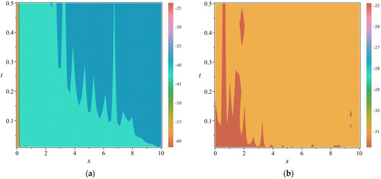
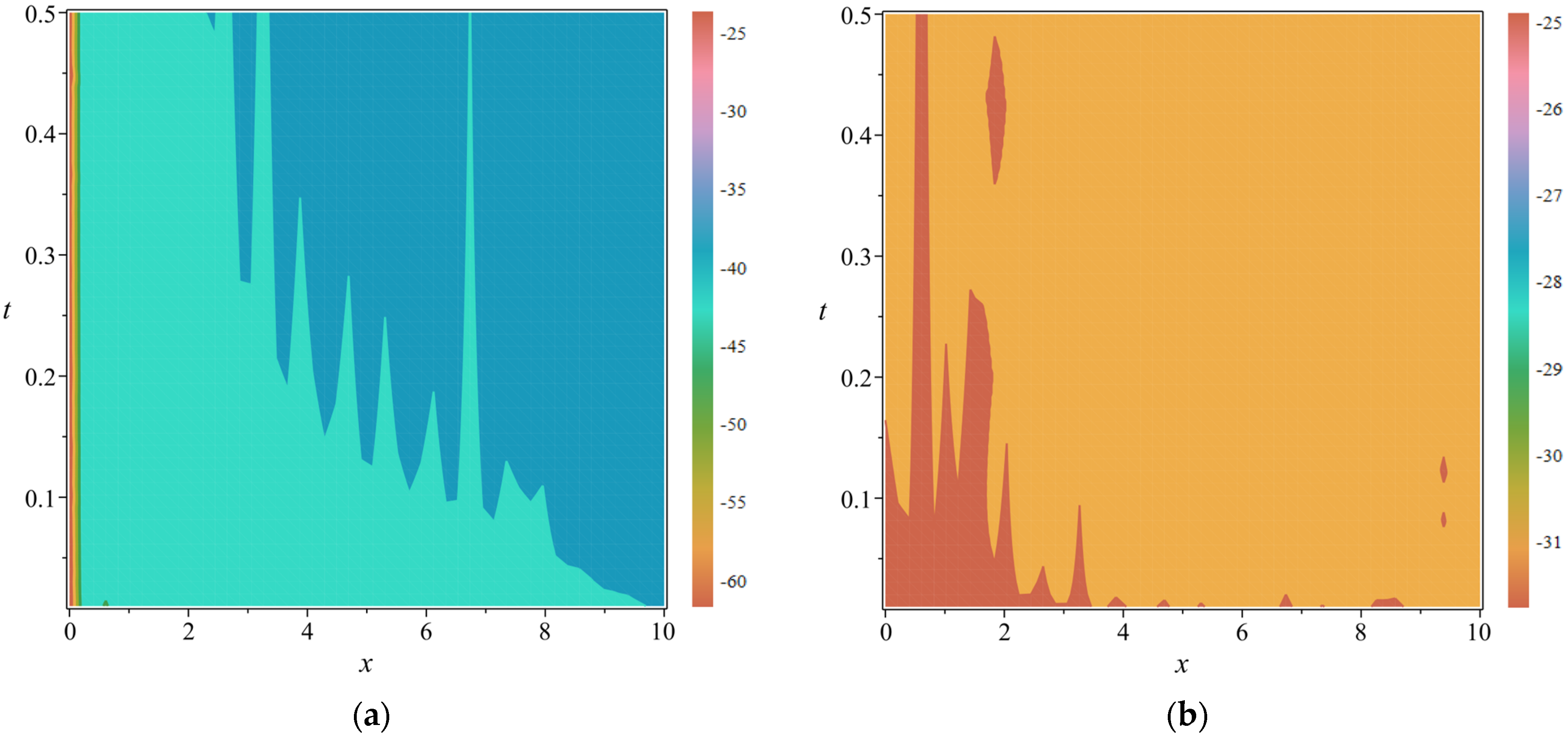
Figure 1. Graphical representations of error indicators for Problem 1 with the specified parameters $(N,M,\delta )=(23,8,0.4)$. (a) Logarithmic plot of the absolute error function: ${log}_{10}\left|v(x,t)-v_{app}^{N,M}(x,t)\right|.$ (b) Logarithmic plot of the absolute residual function: ${log}_{10}\left|{\mathcal{E}}_{N,M}(x,t,\mathit{r})\right|$.

Problem 2. 

For the second test problem, we apply our approach to solve the following fractional Burgers’ equation with variable-order. This is a one-dimensional linear inhomogeneous equation. This renowned Burgers’ equation is used extensively in the simulation of phenomena such as gas dynamics, fluid mechanics, traffic flow, and turbulence:

$${}_0{}^C\mathcal{D}_t^{\alpha \left(t\right)}v(x,t)+{\displaystyle \frac{\partial v(x,t)}{\partial x}}={\displaystyle \frac{{\partial }^{2}v(x,t)}{\partial x^2}}+{\displaystyle \frac{2t^{2-\alpha \left(t\right)}}{\mathrm{\Gamma }(3-\alpha (t\left)\right)}}+2x-2,0<\alpha \left(t\right)<1,$$

(19)

subject to the following initial and boundary conditions:

$$\left\{\begin{array}{cc}v(x,0)=x^2,\hfill & 0\le x\le 1,\hfill \\ v(0,t)=t^2,v(1,t)=1+t^2,\hfill & 0\le t\le 1.\hfill \end{array}\right.$$

The analytical solution of Equation (19) is given by $v(x,t)=x^2+t^2$. In our numerical results, we make the assumption that $\alpha \left(t\right)={\displaystyle \frac{50t+49}{100}}$. Figure 2 shows the graphical representations of error indicators evaluated through our approach, with parameters set as $N=8$, $M=8$, and $\delta =0.4$. Additionally, in Table 3, the reference error, maximum absolute residual error, and relative error of our results across various values of N and M are reported.

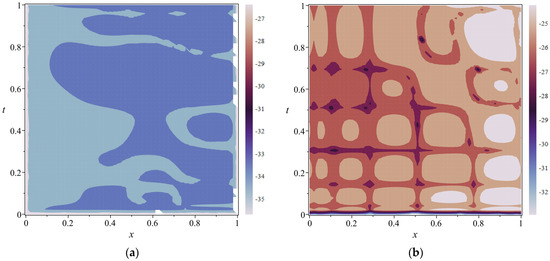
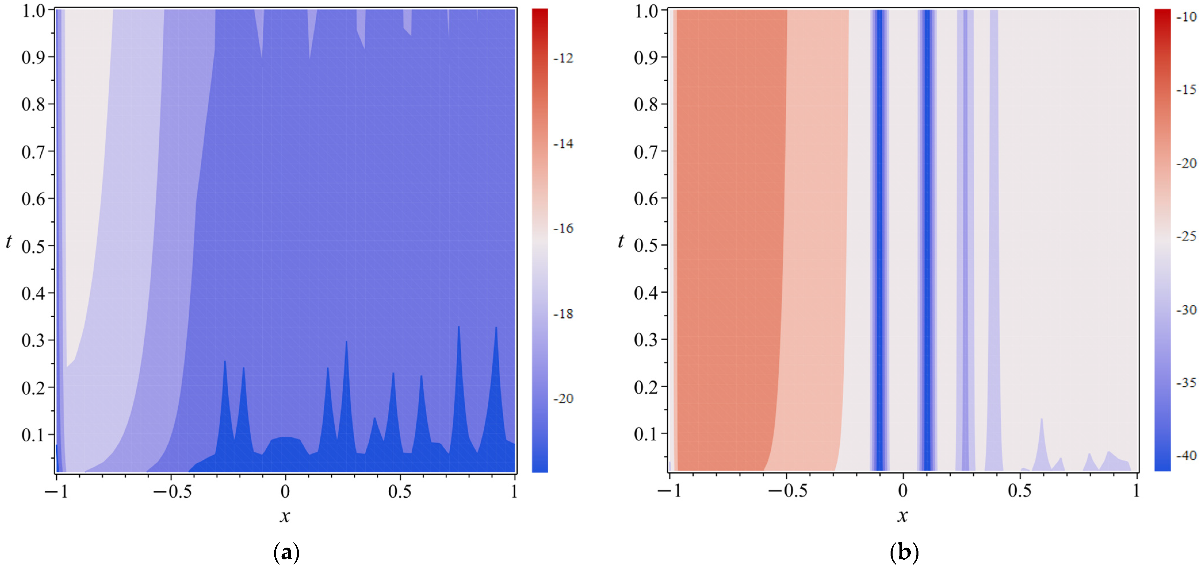
Figure 2. Graphical representations of error indicators for Problem 2 with the specified parameters $(N,M,\delta )=(8,8,0.4)$. (a) Logarithmic plot of the absolute error function: ${log}_{10}\left|v(x,t)-v_{app}^{N,M}(x,t)\right|.$ (b) Logarithmic plot of the absolute residual function: ${log}_{10}\left|{\mathcal{E}}_{N,M}(x,t,\mathit{r})\right|$.

Table 3. Error indicators associated with our obtained results for Problem 2.

$\mathit{\delta }$	N	M	$\mathit{R}.\mathit{E}.(\mathit{N},\mathit{M})$	$\mathit{M}.\mathit{R}.\mathit{E}.(\mathit{N},\mathit{M})$	$\mathbf{Rel}.\mathit{E}.(\mathit{N},\mathit{M})$
0.4	4	1	$3.5059\times {10}^{-01}$	$5.3833\times {10}^{+01}$	$3.7283\times {10}^{-02}$
		2	$3.0927\times {10}^{-02}$	$4.6816\times {10}^{+00}$	$5.6831\times {10}^{-06}$
		3	$6.0000\times {10}^{-30}$	$5.8067\times {10}^{-29}$	$2.5572\times {10}^{-59}$
		4	$5.1000\times {10}^{-30}$	$1.2173\times {10}^{-28}$	$1.1066\times {10}^{-59}$
0.4	6	1	$4.0426\times {10}^{-01}$	$2.9841\times {10}^{+02}$	$3.7557\times {10}^{-02}$
		2	$3.7206\times {10}^{-02}$	$2.5806\times {10}^{+01}$	$1.9739\times {10}^{-04}$
		3	$7.4300\times {10}^{-29}$	$9.5601\times {10}^{-27}$	$4.1602\times {10}^{-58}$
		4	$6.4300\times {10}^{-29}$	$7.4819\times {10}^{-27}$	$7.1249\times {10}^{-58}$
0.4	8	1	$3.9392\times {10}^{-01}$	$9.7281\times {10}^{+02}$	$3.1186\times {10}^{-02}$
		2	$3.5865\times {10}^{-02}$	$8.4053\times {10}^{+01}$	$1.6343\times {10}^{-04}$
		3	$6.9800\times {10}^{-27}$	$1.9503\times {10}^{-25}$	$3.2995\times {10}^{-54}$
		4	$5.0207\times {10}^{-27}$	$3.7009\times {10}^{-25}$	$2.6485\times {10}^{-54}$

Problem 3. 

This problem involves a variable-order time fractional PDE which is a multi-term equation as shown below:

$$\begin{array}{c}\begin{array}{cc}\hfill & {}_0{}^C\mathcal{D}_t^{{\displaystyle \frac{25+t^2}{20}}}v(x,t)+{}_0{}^C\mathcal{D}_t^{{\displaystyle \frac{24+cost}{20}}}v(x,t)+{}_0{}^C\mathcal{D}_t^{{\displaystyle \frac{23+t}{20}}}v(x,t)\hfill \\ \hfill & +{}_0{}^C\mathcal{D}_t^{{\displaystyle \frac{22+sint}{20}}}v(x,t)={\displaystyle \frac{{\partial }^{2}v(x,t)}{\partial x^2}}+f(x,t),\hfill \end{array}\end{array}$$

(20)

with the following conditions:

$$\left\{\begin{array}{cc}v(x,0)=0,{\displaystyle \frac{\partial v(x,0)}{\partial t}}=0,\hfill & -1\le x\le 1,\hfill \\ v(-1,t)=v(1,t)=\left(\mathrm{sech}\left(0.9\right)+\left(\mathrm{sech}1.1\right)\right)t^2,\hfill & 0\le t\le 1.\hfill \end{array}\right.$$

Equation (20) possesses the exact solution $v(x,t)=\left(\mathrm{sech}(x-0.1)+\mathrm{sech}(x+0.1)\right)t^2$, with the following $f(x,t)$:

$$\begin{array}{c}\begin{array}{cc}\hfill f(x,t)& =2\left(\mathrm{sech}(x-0.1)+\mathrm{sech}(x+0.1)\right)[{\displaystyle \frac{t^{\frac{15-t^2}{20}}}{\mathrm{\Gamma }\left(\frac{35-t^2}{20}\right)}}+{\displaystyle \frac{t^{\frac{16-cos\left(t\right)}{20}}}{\mathrm{\Gamma }\left(\frac{36-cos\left(t\right)}{20}\right)}}+{\displaystyle \frac{t^{\frac{17-t}{20}}}{\mathrm{\Gamma }\left(\frac{37-t}{20}\right)}}\hfill \\ & +{\displaystyle \frac{t^{\frac{18-sin\left(t\right)}{20}}}{\mathrm{\Gamma }\left(\frac{38-sin\left(t\right)}{20}\right)}}-{\displaystyle \frac{t^2}{2}}]+2t^2\left({\mathrm{sech}}^3(x-0.1)+{\mathrm{sech}}^3(x+0.1)\right).\hfill \end{array}\end{array}$$

In Table 4, the reference error, maximum absolute residual error, and relative error of our results across various values of N and M are reported. Furthermore, the relative errors are juxtaposed with those documented in [28]. Table 5 illustrates the convergence analysis of our algorithm, providing error indicators and the corresponding experimental order of convergence for our approximations. Additionally, Figure 3 exhibits graphical depictions of error indicators assessed by our proposed method, utilizing parameters $N=28$, $M=28$, and $\delta =0.25$.

Table 4. Error indicators of our approximation and relative error in comparison with [28] for Problem 3.

Presented Method with $\mathit{\delta }=0.25$				Meshless Collocation Method [28] with $\mathit{\delta }=0.25$
$(\mathit{N},\mathit{M})$	$\mathit{R}.\mathit{E}.(\mathit{N},\mathit{M})$	$\mathit{M}.\mathit{R}.\mathit{E}.(\mathit{N},\mathit{M})$	$\mathit{Rel}.\mathit{E}.(\mathit{N},\mathit{M})$	$(\mathit{N},\mathit{k})$	$\mathit{Rel}.\mathit{E}.(\mathit{N},\mathit{k})$
$(8,8)$	$3.1877\times {10}^{-03}$	$5.5490\times {10}^{-02}$	$4.6816\times {10}^{-07}$	$(10,4)$	$3.96\times {10}^{-05}$
$(12,12)$	$3.4328\times {10}^{-05}$	$5.9762\times {10}^{-04}$	$3.3557\times {10}^{-11}$	$(20,4)$	$6.14\times {10}^{-06}$
$(16,16)$	$3.9025\times {10}^{-07}$	$6.7939\times {10}^{-06}$	$3.2339\times {10}^{-15}$	$(40,4)$	$1.12\times {10}^{-06}$
$(20,20)$	$2.6614\times {10}^{-08}$	$4.6333\times {10}^{-07}$	$1.4053\times {10}^{-17}$	$(80,4)$	$1.69\times {10}^{-07}$
$(24,24)$	$5.5820\times {10}^{-10}$	$9.7178\times {10}^{-09}$	$5.6482\times {10}^{-21}$	$(160,4)$	$2.32\times {10}^{-08}$
$(28,28)$	$1.4360\times {10}^{-11}$	$1.8167\times {10}^{-10}$	$2.6389\times {10}^{-24}$	$(320,4)$	$2.99\times {10}^{-09}$

Table 5. Error indicators and their corresponding convergence orders associated with our obtained results for Problem 3.

$\mathit{\delta }$	$(\mathit{N},\mathit{M})$	$\mathit{R}.\mathit{E}.(\mathit{N},\mathit{M})$	${\mathit{r}}_{2,2}^{\mathit{R}.\mathit{E}.(\mathit{N},\mathit{M})}$	$\mathit{M}.\mathit{R}.\mathit{E}.(\mathit{N},\mathit{M})$	${\mathit{r}}_{2,2}^{\mathit{M}.\mathit{R}.\mathit{E}.(\mathit{N},\mathit{M})}$
0.25	(8,8)	$3.1877\times {10}^{-03}$	3.0451	$5.5490\times {10}^{-02}$	3.0449
	(10,10)	$3.8621\times {10}^{-04}$	3.4919	$6.7236\times {10}^{-03}$	3.4919
	(12,12)	$3.4328\times {10}^{-05}$	2.5247	$5.9762\times {10}^{-04}$	5.8467
	(14,14)	$5.9654\times {10}^{-07}$	3.9341	$1.0385\times {10}^{-05}$	0.6122
	(16,16)	$3.9025\times {10}^{-07}$	1.3480	$6.7939\times {10}^{-06}$	1.3480
	(18,18)	$1.5330\times {10}^{-07}$	2.5261	$2.6689\times {10}^{-06}$	2.5261
	(20,20)	$2.6614\times {10}^{-08}$	2.7561	$4.6333\times {10}^{-07}$	2.7561
	(22,22)	$3.9396\times {10}^{-09}$	2.8192	$6.8584\times {10}^{-08}$	2.8192
	(24,24)	$5.5820\times {10}^{-10}$		$9.7178\times {10}^{-09}$

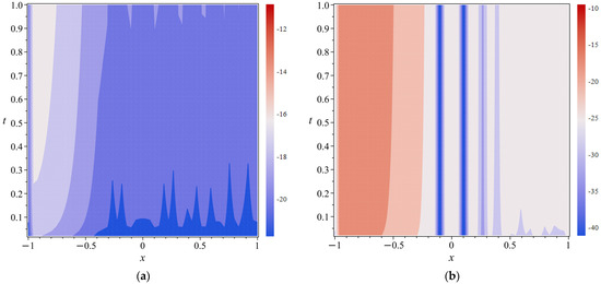
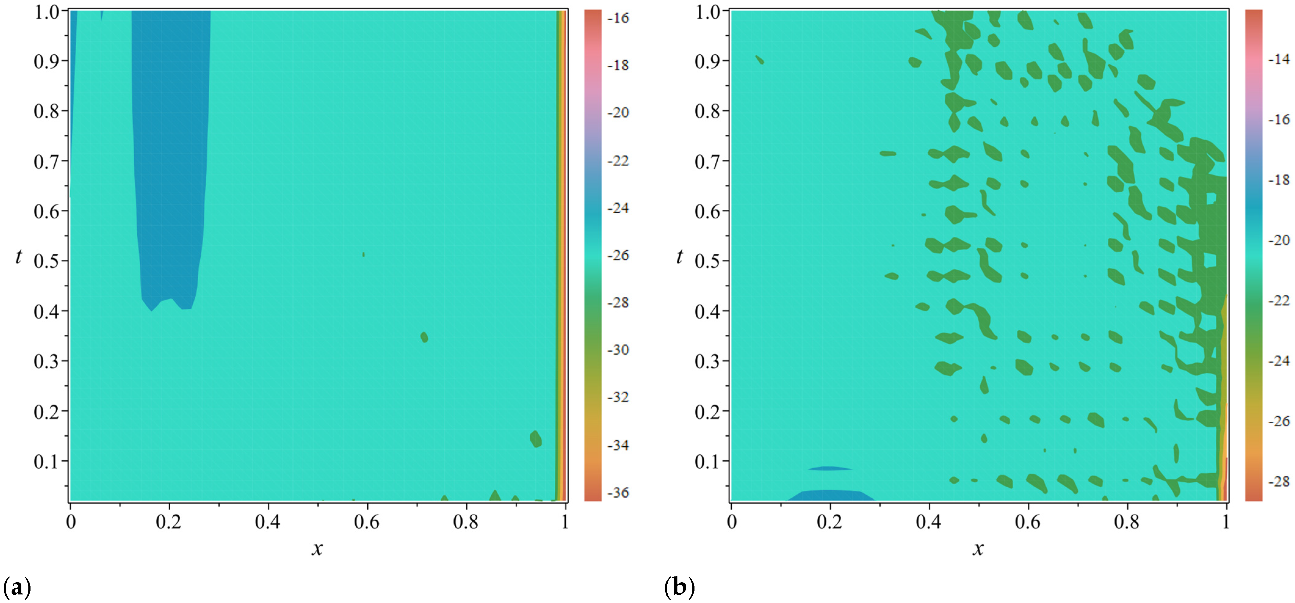
Figure 3. Graphical representations of error indicators for Problem 3 with the specified parameters $(N,M,\delta )=(28,28,0.25)$. (a) Logarithmic plot of the absolute error function: ${log}_{10}\left|v(x,t)-v_{app}^{N,M}(x,t)\right|.$ (b) Logarithmic plot of the absolute residual function: ${log}_{10}\left|{\mathcal{E}}_{N,M}(x,t,\mathit{r})\right|$.

Problem 4. 

Our last variable-order time fractional PDE is:

$${}_0{}^C\mathcal{D}_t^{{\displaystyle \frac{38+t}{20}}}v(x,t)+{}_0{}^C\mathcal{D}_t^{{\displaystyle \frac{8+sint}{5}}}v(x,t)={\displaystyle \frac{{\partial }^{2}v(x,t)}{\partial x^2}}+f(x,t),0\le x\le 1,0\le t\le 1,$$

(21)

with the following conditions:

$$\left\{\begin{array}{cc}v(x,0)={\displaystyle \frac{\partial v(x,0)}{\partial t}}=0,\hfill & 0\le x\le 1,\hfill \\ v(0,t)=exp(-4)t^2,v(1,t)=exp(-64)t^2,\hfill & 0\le t\le 1.\hfill \end{array}\right.$$

Equation (21) possesses the exact solution $v(x,t)=t^{2}exp\left(-100{(x-0.2)}^2\right)$, with the following $f(x,t)$:

$$\begin{array}{c}\begin{array}{cc}\hfill f(x,t)& =2exp\left(-4{(5x-1)}^2\right)\left[{\displaystyle \frac{t^{\frac{2-t}{20}}}{\mathrm{\Gamma }\left(\frac{22-t}{20}\right)}}+{\displaystyle \frac{t^{\frac{2-sin\left(t\right)}{5}}}{\mathrm{\Gamma }\left(\frac{7-sin\left(t\right)}{5}\right)}}-100t^2\left(200x^2-80x+7\right)\right].\hfill \end{array}\end{array}$$

In Table 6, the reference error, maximum absolute residual error, and relative error of our results across various values of N and M are reported. Furthermore, the relative errors are juxtaposed with those documented in [28]. Table 7 illustrates the convergence analysis of our algorithm, providing error indicators and the corresponding experimental order of convergence for our approximations. Additionally, Figure 4 exhibits graphical depictions of error indicators assessed by our proposed method, utilizing parameters $N=25$, $M=25$, and $\delta =1$.

Table 6. Error indicators of our approximation and relative error in comparison with [28] for Problem 4.

Presented Method with $\mathit{\delta }=1$				Meshless Collocation Method [28] with $\mathit{\delta }=1$
$(\mathit{N},\mathit{M})$	$\mathit{R}.\mathit{E}.(\mathit{N},\mathit{M})$	$\mathit{M}.\mathit{R}.\mathit{E}.(\mathit{N},\mathit{M})$	$\mathit{Rel}.\mathit{E}.(\mathit{N},\mathit{M})$	$(\mathit{N},\mathit{k})$	$\mathit{Rel}.\mathit{E}.(\mathit{N},\mathit{k})$
$(8,8)$	$1.6177\times {10}^{-03}$	$5.4111\times {10}^{-02}$	$2.5990\times {10}^{-06}$	$(16,5)$	$7.09\times {10}^{-04}$
$(12,12)$	$1.4687\times {10}^{-06}$	$5.4567\times {10}^{-05}$	$3.2460\times {10}^{-12}$	$(32,5)$	$1.19\times {10}^{-04}$
$(16,16)$	$1.0544\times {10}^{-09}$	$8.8332\times {10}^{-08}$	$9.0815\times {10}^{-19}$	$(64,5)$	$3.31\times {10}^{-05}$
$(20,20)$	$9.3629\times {10}^{-13}$	$1.3710\times {10}^{-10}$	$1.7478\times {10}^{-24}$	$(128,5)$	$2.11\times {10}^{-06}$
$(24,24)$	$8.3417\times {10}^{-16}$	$4.1830\times {10}^{-13}$	$1.2302\times {10}^{-30}$	$(256,5)$	$5.04\times {10}^{-07}$

Table 7. Error indicators and their corresponding convergence orders associated with our obtained results for Problem 4.

$\mathit{\delta }$	$(\mathit{N},\mathit{M})$	$\mathit{R}.\mathit{E}.(\mathit{N},\mathit{M})$	${\mathit{r}}_{2,2}^{\mathit{R}.\mathit{E}.(\mathit{N},\mathit{M})}$	$\mathit{M}.\mathit{R}.\mathit{E}.(\mathit{N},\mathit{M})$	${\mathit{r}}_{2,2}^{\mathit{M}.\mathit{R}.\mathit{E}.(\mathit{N},\mathit{M})}$
1	(8,8)	$1.6177\times {10}^{-03}$	2.1598	$5.4111\times {10}^{-02}$	2.7559
	(10,10)	$3.6203\times {10}^{-04}$	7.9454	$8.0108\times {10}^{-03}$	7.1978
	(12,12)	$1.4687\times {10}^{-06}$	4.8439	$5.4567\times {10}^{-05}$	4.7305
	(14,14)	$5.1142\times {10}^{-08}$	5.6000	$2.0554\times {10}^{-06}$	4.5403
	(16,16)	$1.0544\times {10}^{-09}$	5.4143	$8.8332\times {10}^{-08}$	4.3594
	(18,18)	$2.4725\times {10}^{-11}$	4.7229	$4.3035\times {10}^{-09}$	4.9722
	(20,20)	$9.3629\times {10}^{-13}$	7.4682	$1.3710\times {10}^{-10}$	2.9650
	(22,22)	$5.2877\times {10}^{-15}$	2.6642	$1.7558\times {10}^{-11}$	5.3914
	(24,24)	$8.3417\times {10}^{-16}$		$4.1830\times {10}^{-13}$

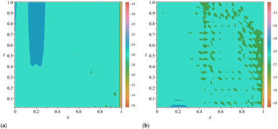
Figure 4. Graphical representations of error indicators for Problem 4 with the specified parameters $(N,M,\delta )=(25,25,1)$. (a) Logarithmic plot of the absolute error function: ${log}_{10}\left|v(x,t)-v_{app}^{N,M}(x,t)\right|.$ (b) Logarithmic plot of the absolute residual function: ${log}_{10}\left|{\mathcal{E}}_{N,M}(x,t,\mathit{r})\right|$.

Based on the findings presented in Table 1, Table 2, Table 3, Table 4, Table 5, Table 6 and Table 7, it is evident that the maximum absolute values of error indicators exhibit a rapid decrease with increasing values of N or M. Moreover, the reported experimental convergence order in the tables underscores the efficacy and dependability of the proposed method.

6. Conclusions

We presented a novel and efficient algorithm aimed at dealing with the variable-order in space and time of fractional PDEs in their most general form. This encompasses a comprehensive investigation of these equations and their associated boundary conditions, formulated in a generalized framework. Our method involves approximating the solution of the governing equation using a combination of shifted Chebyshev polynomials with time-dependent coefficients. Through the integration of boundary conditions and the application of collocation methods, we have determined these coefficients. Theoretical analysis and numerical experiments corroborated the effectiveness and efficiency of our approach. Consequently, our method can be a suitable algorithm for addressing a wide range of differential equations.

References

- Diethelm, K. The Analysis of Fractional Differential Equations; Springer: Berlin/Heidelberg, Germany, 2010. [Google Scholar]
- Ross, B.; Samko, S. Integration and differentiation to a variable fractional order. Integral Transform. Spec. Funct. 1993, 1, 277–300. [Google Scholar] [CrossRef]
- Samko, S. Fractional integration and differentiation of variable order. Anal. Math. 1995, 21, 213–236. [Google Scholar] [CrossRef]
- Sun, H.; Chen, W.; Wei, H.; Chen, Y. A comparative study of constant-order and variable-order fractional models in characterizing memory property of systems. Eur. Phys. J. Spec. Top. 2011, 193, 185–192. [Google Scholar] [CrossRef]
- Samko, S. Fractional integration and differentiation of variable order: An overview. Nonlinear Dyn. 2013, 71, 653–662. [Google Scholar] [CrossRef]
- Almeida, R.; Tavares, D.; Torres, D.F.M. The Variable-Order Fractional Calculus of Variations; Springer: Berlin/Heidelberg, Germany, 2019. [Google Scholar]
- Chechkin, A.; Gorenflo, R.; Sokolov, I. Fractional diffusion in inhomogeneous media. J. Phys. Math. Gen. 2005, 38, L679–L684. [Google Scholar] [CrossRef]
- Zheng, X.; Wang, H.; Fu, H. Analysis of a physically-relevant variable-order time-fractional reaction–diffusion model with mittag-leffler kernel. Appl. Math. Lett. 2021, 112, 106804. [Google Scholar] [CrossRef]
- Guo, X.; Zheng, X. Variable-order time-fractional diffusion equation with mittag-leffler kernel: Regularity analysis and uniqueness of determining variable order. Z. FÜR Angew. Math. Phys. ZAMP 2023, 74, 64–68. [Google Scholar] [CrossRef]
- Coimbra, C. Mecganics with variable-order differential operators. Ann. Der Phys. 2001, 12, 692–703. [Google Scholar] [CrossRef]
- Orosco, J.; Coimbra, C. On the control and stability of variable-order mechanical systems. Nonlinear Dyn. 2016, 86, 695–710. [Google Scholar] [CrossRef]
- Ganji, R.M.; Jafari, H.; Adem, A.R. A numerical scheme to solve variable order diffusion-wave equations. Therm. Sci. 2019, 23, S2063–S2071. [Google Scholar] [CrossRef]
- Ganji, R.; Jafari, H. A numerical approach for multi-variable orders differential equations using jacobi polynomials. Int. J. Applied Comput. Math. 2019, 5, 34. [Google Scholar] [CrossRef]
- Ganji, R.; Jafari, H.; Baleanu, D. A new approach for solving multi variable orders differential equations with mittag-leffler kernel. Chaos Solitons Fractals 2020, 130, 109405. [Google Scholar] [CrossRef]
- Doha, E.H.; Abdelkawy, M.A.; Amin, A.Z.M.; Baleanu, D. Spectral technique for solving variable-order fractional volterra integro-differential equations. Numer. Methods Partial. Differ. Equ. 2018, 34, 1659–1677. [Google Scholar] [CrossRef]
- Chen, Y.-M.; Wei, Y.-Q.; Liu, D.-Y.; Yu, H. Numerical solution for a class of nonlinear variable order fractional differential equations with legendre wavelets. Appl. Math. Lett. 2015, 46, 83–88. [Google Scholar] [CrossRef]
- Xu, Y.; Ertürk, V.S. A finite difference technique for solving variable-order fractional integro-differential equations. Bull. Iran. Soc. 2014, 40, 699–712. [Google Scholar]
- Yang, J.; Yao, H.; Wu, B. An efficient numerical method for variable order fractional functional differential equation. Appl. Math. 2018, 76, 221–226. [Google Scholar] [CrossRef]
- Jafari, H.; Tajadodi, H.; Ganji, R.M. A numerical approach for solving variable order differential equations based on bernstein polynomials. Comput. Math. Methods 2019, 1, e1055. [Google Scholar] [CrossRef]
- Tavares, D.; Almeida, R.; Torres, D.F. Caputo derivatives of fractional variable order: Numerical approximations. Commun. Nonlinear Sci. Numer. Simul. 2016, 35, 69–87. [Google Scholar] [CrossRef]
- Santamaria, F.; Wils, S.; Schutter, E.D.; Augustine, G.J. Anomalous diffusion in purkinje cell dendrites caused by spines. Neuron 2006, 52, 635–648. [Google Scholar] [CrossRef]
- Sun, H.; Chen, W.; Chen, Y. Variable-order fractional differential operators in anomalous diffusion modeling. Phys. Stat. Mech. Its Appl. 2009, 388, 4586–4592. [Google Scholar] [CrossRef]
- Kheybari, S. Numerical algorithm to Caputo type time-space fractional partial differential equations with variable coefficients. Math. Comput. Simul. 2021, 182, 66–85. [Google Scholar] [CrossRef]
- Kheybari, S.; Darvishi, M.T.; Hashemi, M.S. A semi-analytical approach to caputo type time-fractional modified anomalous sub-diffusion equations. Appl. Numer. Math. 2020, 158, 103–122. [Google Scholar] [CrossRef]
- Shen, J.; Tang, T.; Wang, L.-L. Spectral Methods: Algorithms, Analysis and Applications; Springer Science & Business Media: Cham, The Netherland, 2011; Volume 41. [Google Scholar]
- Gottlieb, D.; Orszag, S.A. Numerical Analysis of Spectral Methods, Theory and Applications; SIAM-CBMS: Philadelphia, PA, USA, 1977. [Google Scholar] [CrossRef]
- Sun, H.; Chen, W.; Li, C.; Chen, Y. Finite difference schemes for variable-order time fractional diffusion equation. Int. J. Bifurc. Chaos 2012, 22, 1250085. [Google Scholar] [CrossRef]
- Tian, X.; Reutskiy, S.Y.; Fu, Z.-J. A novel meshless collocation solver for solving multi-term variable-order time fractional pdes. Eng. Comput. 2021, 38, 1527–1538. [Google Scholar] [CrossRef]
Disclaimer/Publisher’s Note: The statements, opinions and data contained in all publications are solely those of the individual author(s) and contributor(s) and not of MDPI and/or the editor(s). MDPI and/or the editor(s) disclaim responsibility for any injury to people or property resulting from any ideas, methods, instructions or products referred to in the content. |
© 2024 by the authors. Licensee MDPI, Basel, Switzerland. This article is an open access article distributed under the terms and conditions of the Creative Commons Attribution (CC BY) license (https://creativecommons.org/licenses/by/4.0/).