Spectral Galerkin Methods for Riesz Space-Fractional Convection–Diffusion Equations

Abstract

This paper applies the spectral Galerkin method to numerically solve Riesz space-fractional convection–diffusion equations. Firstly, spectral Galerkin algorithms were developed for one-dimensional Riesz space-fractional convection–diffusion equations. The equations were solved by discretizing in space using the Galerkin–Legendre spectral approaches and in time using the Crank–Nicolson Leap-Frog (CNLF) scheme. In addition, the stability and convergence of semi-discrete and fully discrete schemes were analyzed. Secondly, we established a fully discrete form for the two-dimensional case with an additional complementary term on the left and then obtained the stability and convergence results for it. Finally, numerical simulations were performed, and the results demonstrate the effectiveness of our numerical methods.

1. Introduction

Fractional calculus theory is a generalization of traditional calculus theory that extends the order of derivatives from integers to real numbers. Compared with conventional differential equations, fractional differential equations can better simulate physical processes in nature due to the non-locality of the fractional derivatives. Fractional differential equations have been extensively researched in various fields, including mechanics, statistics, physics, biology, economics, and finance [1,2,3,4,5,6,7,8].

Fractional differential equations are typically challenging to solve due to the non-locality of fractional differential operators. Some fractional differential equations can be solved using the Fourier transform, Laplace transform, Mellin transform, or Green function [9,10,11,12]. However, these solutions typically involve complex and specialized functions that are challenging to calculate, such as Mittag-Leffler functions, Wright functions, hypergeometric functions, etc. As a matter of fact, for the vast majority of fractional differential equations, the analytical solution cannot be found. Therefore, it is crucial to develop efficient and stable numerical algorithms for them. Numerical algorithms for fractional differential equations mainly include the finite difference method, finite element method, and spectral method. The spectral method differs from the first two methods in that it utilizes trigonometric functions or orthogonal polynomials as basis functions for numerical approximation, which contributes to its high convergence. The higher the regularity of the true solution, the smaller the error of the numerical solution. If the exact solution of the equation is infinitely smooth, then the spectral method can achieve convergence accuracy of “infinite order”. In 1994, Blinova proposed the concept of spectral methods. In the 1980s, Gottlieb et al. extended the spectral method to solve a wide range of problems and conducted systematic theoretical analysis. In the 1990s, spectral methods were widely used in fluid mechanics calculations [13].

The fractional convection–diffusion equation is a significant application of fractional partial differential equations and is extensively utilized in science and engineering. Fractional differential equations can be directly used to describe anomalous diffusion phenomena [14]. The non-Gaussian diffusion process can be described using fractional derivatives, such as the Caputo fractional derivative, the Riemann–Liouville fractional derivative, or the Riesz fractional derivative [15,16]. In general, the Caputo derivative is often used in the temporal domain to represent the historical dependence in the time direction. The Riemann–Liouville derivatives or Riesz fractional derivatives are often used in the spatial direction to characterize long-distance interactions [17,18,19,20].

The Riesz fractional derivatives on a finite domain $[a,b]$ are defined as follows:

$$\begin{array}{cc}\hfill \frac{{\partial }^{\gamma }u}{{\partial \left|x\right|}^{\gamma }}& =c_{\gamma }\left({}_{a}D_x^{\gamma }u+{}_{x}D_b^{\gamma }u\right),0<\gamma <2,\gamma \ne 1,\hfill \end{array}$$

where $c_{\gamma }=-1/\left(2\cos (\gamma \pi /2)\right)$, and for $n-1\le \gamma <n,n\in \mathbb{N}$, the operators ${}_{a}D_x^{\gamma }$, ${}_{x}D_b^{\gamma }$ are

$$\begin{array}{cc}\hfill {}_{a}D_x^{\gamma }u& =\frac{1}{\mathsf{\Gamma }(n-\gamma )}\frac{{\partial }^n}{\partial x^n}{\int }_a^x\frac{u\left(s\right)}{{(x-s)}^{\gamma -n+1}}ds,\hfill \\ \hfill {}_{x}D_b^{\gamma }u& =\frac{{(-1)}^n}{\mathsf{\Gamma }(n-\gamma )}\frac{{\partial }^n}{\partial x^n}{\int }_x^b\frac{u\left(s\right)}{{(s-x)}^{\gamma -n+1}}ds.\hfill \end{array}$$

From the above definition, we can see that the Riesz fractional derivative includes both left and right Riemann–Liouville fractional derivatives. This indicates that a state depends on information not only on the left side but also on the right side. For more details, please refer to [1].

There have been numerous studies on the numerical solution of fractional-order (convection–) diffusion equations: Sun [21] used the $L1$ formula to approximate the time derivative and presented a difference scheme for the Caputo time-fractional diffusion-wave equation. Liu [22] proposed a random walk model to approximate the Lévy–Feller advection–dispersion process and provided an explicit finite difference approximation of the equation. Shen [23] used the shifted Grünward–Letnikov formula to approximate the spatial-fractional derivative, and the $L1$ formula to approximate the temporal fractional derivative. Shen provided explicit and implicit differences for the space–time Riesz-Caputo fractional advection–diffusion equation. Zhou [24] proposed a compact finite difference scheme for the space-fractional diffusion equation. Wang [25] proposed a fast characteristic finite difference method for solving space-fractional advection–diffusion equations. Huang [26] provided the finite element solution for the fractional advection–dispersion equation. Lai [27] obtained a space–time finite element method for linear Riesz space-fractional partial differential equations. Tang [28] proposed the discontinuous Galerkin method combined with the Runge–Kutta method for solving the spatial-fractional diffusion equation. Bhrawy [29] utilized the shifted Jacobi polynomial as the basis function to construct a matrix of fractional differential operators and proposed a Jacobi spectral collocation method for nonlinear fractional sub-diffusion equations. Afterward, Bhrawy [30] introduced the spectral tau method for the two-sided space–time Caputo fractional diffusion-wave equation. This method utilized the shifted Legendre polynomial as the basis function to construct a fractional differential matrix. Saadatmandi [31] utilized the Sinc–Legendre configuration method to provide a numerical approximation of a series of variable-coefficient fractional convection–diffusion equations.

For the convection–diffusion equation with Riesz fractional derivatives, Shen [32] utilized the Laplace transform and Fourier transform to derive the exact solution of the Riesz space-fractional convection–diffusion equation. Additionally, the finite difference formulation is provided using the Grünward–Letnikov formula. Yang [33] established the relationship between the Laplace operator and the Riesz fractional differential operator and used the eigenequation $-\Delta \varphi =\lambda \varphi$ to derive the analytical solution of the Riesz spatial diffusion equation. Moreover, the $L1$ / $L2$ approximation method, the displacement Grünward formula method, and the matrix transformation method (MTM) were employed to approximate the fractional derivative. Zhang [34] proposed the Galerkin finite element approximation of the Riesz space-fractional convection–diffusion equation. Celik [35] presented the Crank–Nicolson method for solving the Riesz space-fractional diffusion equation. Zeng [36] proposed the Crank–Nicolson Alternating Direction Implicit (ADI) method for solving the Riesz nonlinear reaction–diffusion equation. Anley [37] discussed the finite difference method for a two-sided two-dimensional space-fractional convection–diffusion problem with a source term. Basha [38] derived a linearized Crank–Nicolson scheme for the two-dimensional nonlinear Riesz space-fractional convection–diffusion equation.

Recently, some researchers have been exploring numerical solutions for distribution-order differential equations. For example, Li [39,40] considered the finite volume method for the Riesz spatial distribution-order diffusion equation and the convection–diffusion equation, respectively. Ye [41] presented an implicit difference scheme for time distributed-order and Riesz space-fractional diffusion equations. Zhang [42] proposed the Crank–Nicolson ADI Galerkin–Legendre spectral method for solving the two-dimensional Riesz space distributed-order advection–diffusion equation. Hu [43] introduced a new definition of the spatial derivative and provided the implicit difference scheme for the space-fractional advection–dispersion equation.

In this paper, we consider the below Riesz space-fractional convection–diffusion equations [37,44]:

$$\begin{array}{cc}\hfill \frac{\partial u(\mathit{x},t)}{\partial t}& =\sum _{i=1}^d{K}_i\frac{{\partial }^{{\gamma }_i^{\left(1\right)}}u(\mathit{x},t)}{\partial |x_i{|}^{{\gamma }_i^{\left(1\right)}}}+\sum _{i=1}^d{K}_{d+i}\frac{{\partial }^{{\gamma }_i^{\left(2\right)}}u(\mathit{x},t)}{\partial |x_i{|}^{{\gamma }_i^{\left(2\right)}}}+f(\mathit{x},t),(\mathit{x},t)\in {\mathsf{\Omega }}_d\times I,\hfill \\ \hfill u(\mathit{x},0)& =u_0\left(\mathit{x}\right),\mathit{x}\in {\mathsf{\Omega }}_d,\hfill \\ \hfill u(\mathit{x},t)& =0,(\mathit{x},t)\in \partial {\mathsf{\Omega }}_d\times I,\hfill \end{array}$$

(1)

where $0<{\gamma }_i^{\left(1\right)}<1$, $1<{\gamma }_i^{\left(2\right)}<2$, $I=(0,T]$ is the time interval, ${\mathsf{\Omega }}_d=(a_1,b_1)\times \cdots \times (a_d,b_d)$ is the d-dimensional spatial domain, $u(\mathit{x},t)$ denotes the solute concentration, positive numbers of $K_i,i=1,\cdots ,d$ denote the fluid velocities in the $x_i$ direction, positive numbers of $K_{d+i},i=1,\cdots ,d$ denote the diffusion coefficients, and $f(\mathit{x},t)$ is the source function.

We aim to apply the spectral Galerkin method to the above Riesz space-fractional convection–diffusion equations when $d=1$ and $d=2$ and derive a fast and efficient scheme for those equations. This paper is structured as follows. In Section 2, preliminaries for fractional derivatives are introduced. In Section 3 and Section 4, the spectral Galerkin methods for solving one-dimensional and two-dimensional space-fractional convection–diffusion equations are presented, together with the analysis of the stability and convergence, respectively. Several numerical examples are provided in Section 5, and the results of these examples can validate the effectiveness of the proposed algorithms. This paper is summarized in Section 6.

2. Preliminaries

In this section, we will introduce the necessary notations and details in fractional calculus that are used throughout this paper.

Lemma 1.

If $n-1<\alpha <n$, $\hat{x}\in [-1,1]$, then

$$\begin{array}{c}\hfill {}_{-1}D_{\hat{x}}^{\alpha }\left({(1+\hat{x})}^{\delta +\alpha }{J}_n^{\gamma -\alpha ,\delta +\alpha }\left(\hat{x}\right)\right)=\frac{\mathsf{\Gamma }(n+\delta +\alpha +1)}{\mathsf{\Gamma }(n+\delta +1)}{(1+x)}^{\delta }{J}_n^{\gamma ,\delta }\left(\hat{x}\right),\\ \hfill {}_{\hat{x}}D_1^{\alpha }\left({(1-\hat{x})}^{\gamma +\alpha }{J}_n^{\gamma +\alpha ,\delta -\alpha }\left(\hat{x}\right)\right)=\frac{\mathsf{\Gamma }(n+\gamma +\alpha +1)}{\mathsf{\Gamma }(n+\gamma +1)}{(1-x)}^{\gamma }{J}_n^{\gamma ,\delta }\left(\hat{x}\right),\end{array}$$

where $J_n^{\alpha ,\beta }\left(\hat{x}\right)(\alpha ,\beta >-1)$ is the Jacobi polynomial [45].

According to Lemma 1, the chain rule, and $L_n\left(\hat{x}\right)=J_n^{0,0}\left(\hat{x}\right)$, we have the following lemma.

Lemma 2.

If $n-1<\alpha <n$, $\hat{x}\in [-1,1]$, $x=(b-a)\hat{x}/2+(b+a)/2\in [a,b]$, then

$$\begin{array}{cc}\hfill {}_{a}D_x^{\alpha }{L}_n\left(\hat{x}\right)& =\frac{1}{\mathsf{\Gamma }(n-\alpha )}\frac{d^n}{d{x}^n}{\int }_a^x{(x-s)}^{n-\alpha -1}{L}_n\left(\hat{x}\right)ds\hfill \\ & ={(\frac{b-a}{2})}^{-\alpha }\frac{\mathsf{\Gamma }(n+1)}{\mathsf{\Gamma }(n-\alpha +1)}{(1+\hat{x})}^{-\alpha }{J}_n^{\alpha ,-\alpha }\left(\hat{x}\right),\hat{x}\in [-1,1],\hfill \\ \hfill {}_{x}D_b^{\alpha }{L}_n\left(\hat{x}\right)& =\frac{{(-1)}^n}{\mathsf{\Gamma }(n-\alpha )}\frac{d^n}{d{x}^n}{\int }_x^b{(s-x)}^{n-\alpha -1}{L}_n\left(\hat{x}\right)ds\hfill \\ & ={(\frac{b-a}{2})}^{-\alpha }\frac{\mathsf{\Gamma }(n+1)}{\mathsf{\Gamma }(n-\alpha +1)}{(1-\hat{x})}^{-\alpha }{J}_n^{-\alpha ,\alpha }\left(\hat{x}\right),\hat{x}\in [-1,1],\hfill \end{array}$$

where $L_n\left(\hat{x}\right)$ is the Legendre polynomial [45], and $J_n^{\alpha ,\beta }\left(\hat{x}\right)(\alpha ,\beta >-1)$ is the Jacobi polynomial.

Let d denote the dimensionality of the space. We choose ${\mathsf{\Omega }}_d=(a_1,b_1)\times \cdots \times (a_d,b_d)\subset {\mathbb{R}}^d$ to be the space domain with $d=1$ or $d=2$ in this paper. Let ${\mathcal{L}}^2\left({\mathsf{\Omega }}_d\right)$ denote the ${\mathcal{L}}^2$-space on ${\mathsf{\Omega }}_d$, with the corresponding inner product being $(·,·)$ and the ${\mathcal{L}}^2$-norm being ${\parallel ·\parallel }_{{\mathcal{L}}^2\left({\mathsf{\Omega }}_d\right)}$. $C_0^{\infty }\left({\mathsf{\Omega }}_d\right)$ denotes the space consisting of all infinitely many successive differentiable functions on ${\mathsf{\Omega }}_d$ with compact support. In the following, we present several function spaces.

Definition 1.

Define the seminorm

$${\left|u\right|}_{J_L^{\mu }\left({\mathsf{\Omega }}_d\right)}={\left(\sum _{i=1}^d{\parallel {}_{a_i}D_{x_i}^{\mu }u\left(\mathit{x}\right)\parallel }_{{\mathcal{L}}^2\left({\mathsf{\Omega }}_d\right)}^2\right)}^{1/2},$$

and the norm

$${\parallel u\parallel }_{J_L^{\mu }\left({\mathsf{\Omega }}_d\right)}={\left({\parallel u\parallel }_{{\mathcal{L}}^2\left({\mathsf{\Omega }}_d\right)}^2+{\left|u\right|}_{J_L^{\mu }\left({\mathsf{\Omega }}_d\right)}^2\right)}^{1/2},$$

for $\mu >0$. Here, $J_L^{\mu }\left({\mathsf{\Omega }}_d\right)$ ($J_{L,0}^{\mu }\left({\mathsf{\Omega }}_d\right)$) denotes the closure of $C^{\infty }\left({\mathsf{\Omega }}_d\right)$ ($C_0^{\infty }\left({\mathsf{\Omega }}_d\right)$) with respect to ${\parallel ·\parallel }_{J_L^{\mu }\left({\mathsf{\Omega }}_d\right)}$.

Definition 2.

Define the seminorm

$${\left|u\right|}_{J_R^{\mu }\left({\mathsf{\Omega }}_d\right)}={\left(\sum _{i=1}^d{\parallel {}_{x_i}D_{b_i}^{\mu }u\left(\mathit{x}\right)\parallel }_{{\mathcal{L}}^2\left({\mathsf{\Omega }}_d\right)}^2\right)}^{1/2},$$

and the norm

$${\parallel u\parallel }_{J_R^{\mu }\left({\mathsf{\Omega }}_d\right)}={\left({\parallel u\parallel }_{{\mathcal{L}}^2\left({\mathsf{\Omega }}_d\right)}^2+{\left|u\right|}_{J_R^{\mu }\left({\mathsf{\Omega }}_d\right)}^2\right)}^{1/2},$$

for $\mu >0$. Here, $J_R^{\mu }\left({\mathsf{\Omega }}_d\right)$ ($J_{R,0}^{\mu }\left({\mathsf{\Omega }}_d\right)$) denotes the closure of $C^{\infty }\left({\mathsf{\Omega }}_d\right)$ ($C_0^{\infty }\left({\mathsf{\Omega }}_d\right)$) with respect to ${\parallel ·\parallel }_{J_R^{\mu }\left({\mathsf{\Omega }}_d\right)}$.

Definition 3.

Define the seminorm

$${\left|u\right|}_{J_S^{\mu }\left({\mathsf{\Omega }}_d\right)}={\left(\sum _{i=1}^d\left|({}_{a_i}D_{x_i}^{\mu }u\left(\mathit{x}\right),{}_{x_i}D_{b_i}^{\mu }u\left(\mathit{x}\right))\right|\right)}^{1/2}$$

and the norm

$${\parallel u\parallel }_{J_S^{\mu }\left({\mathsf{\Omega }}_d\right)}={\left({\parallel u\parallel }_{{\mathcal{L}}^2\left({\mathsf{\Omega }}_d\right)}^2+{\left|u\right|}_{J_S^{\mu }\left({\mathsf{\Omega }}_d\right)}\right)}^{1/2},$$

for $\mu >0$. Here, $J_S^{\mu }\left({\mathsf{\Omega }}_d\right)$ ($J_{S,0}^{\mu }\left({\mathsf{\Omega }}_d\right)$) denotes the closure of $C^{\infty }\left({\mathsf{\Omega }}_d\right)$ ($C_0^{\infty }\left({\mathsf{\Omega }}_d\right)$) with respect to ${\parallel ·\parallel }_{J_S^{\mu }\left({\mathsf{\Omega }}_d\right)}$.

Definition 4

([46]). Define the seminorm

$${\left|u\right|}_{H^{\mu }\left({\mathsf{\Omega }}_d\right)}=\parallel {\left|\omega \right|}^{\mu }\mathit{F}\left(u\right)\left(\omega \right){\parallel }_{{\mathcal{L}}^2\left({\mathbb{R}}^d\right)}$$

and the norm

$${\parallel u\parallel }_{H^{\mu }\left({\mathsf{\Omega }}_d\right)}={\left({\parallel u\parallel }_{{\mathcal{L}}^2\left({\mathsf{\Omega }}_d\right)}^2+{\left|u\right|}_{H^{\mu }\left({\mathsf{\Omega }}_d\right)}\right)}^{1/2},$$

for $\mu >0$, where $\mathit{F}\left(u\right)\left(\omega \right)$ is the Fourier transform of the function $u\left(\mathit{x}\right)$. $H_0^{\mu }\left({\mathsf{\Omega }}_d\right)$ denotes the closure of $C_0^{\infty }$ with respect to ${\parallel ·\parallel }_{H^{\mu }\left({\mathsf{\Omega }}_d\right)}$.

Lemma 3

([42]). Let $\mu >0$ and $\mathsf{\Omega }=(a,b)$, $\forall u\in H_0^{\mu }\left(\mathsf{\Omega }\right)$, $v\in H_0^{\mu /2}\left(\mathsf{\Omega }\right)$. We have

$$\left({}_{a}D_x^{\mu }u,v\right)=\left({}_{a}D_x^{\mu /2}u,{}_{x}D_b^{\mu /2}v\right),\left({}_{x}D_b^{\mu }u,v\right)=\left({}_{x}D_b^{\mu /2}u,{}_{a}D_x^{\mu /2}v\right).$$

Lemma 4.

Let $\mu >0$, $\mu \ne n-1/2$, $n\in \mathbb{N}$. The spaces $J_{L,0}^{\mu }\left({\mathsf{\Omega }}_d\right)$, $J_{R,0}^{\mu }\left({\mathsf{\Omega }}_d\right)$, and $J_{S,0}^{\mu }\left({\mathsf{\Omega }}_d\right)$ are equivalent to $H_0^{\mu }\left({\mathsf{\Omega }}_d\right)$ and have equivalent norms and seminorms.

Lemma 5

([36]). Let $\mu >0$ and $\mathsf{\Omega }=(a,b)$ for $u\in J_{L,0}^{\mu }\left(\mathsf{\Omega }\right)\bigcap J_{R,0}^{\mu }\left(\mathsf{\Omega }\right)$; then,

$$\left({}_{a}D_x^{\mu }u,{}_{x}D_b^{\mu }u\right)=\cos \left(\mu \pi \right)\parallel {}_{-\infty }D_x^{\mu }\hat{u}{\parallel }_{{\mathcal{L}}^2\left(\mathbb{R}\right)}^2=\cos \left(\mu \pi \right){\parallel {}_{x}D_{\infty }^{\mu }\hat{u}\parallel }_{{\mathcal{L}}^2\left(\mathbb{R}\right)}^2,$$

where $\hat{u}$ is the extension of u by zero outside Ω. If $\mu \ne n-1/2$, $n\in \mathbb{N}$ and $u\in J_{L,0}^{\mu }\left(\mathsf{\Omega }\right)$, then there exists a constant C independent of u such that

$$|\hat{u}{|}_{J_L^{\mu }\left(\mathbb{R}\right)}\le C{\left|u\right|}_{J_L^{\mu }\left(\mathsf{\Omega }\right)}.$$

Note that there are also results similar to the above lemma for the two-dimensional case. Please refer to [36].

Lemma 6

([36]). Let $\mu >0$. If $u\in H_0^{\mu }\left({\mathsf{\Omega }}_d\right)$, then there exists a constant $C_1<1$ such that

$$C_1{\parallel u\parallel }_{H_0^{\mu }\left({\mathsf{\Omega }}_d\right)}\le {\left|u\right|}_{H_0^{\mu }\left({\mathsf{\Omega }}_d\right)}\le {\parallel u\parallel }_{H_0^{\mu }\left({\mathsf{\Omega }}_d\right)}.$$

3. Spectral Galerkin Methods for One-Dimensional Riesz Space-Fractional Convection–Diffusion Equation

In this section, we focus on the following one-dimensional Riesz space-fractional convection–diffusion equation for $0<{\alpha }_1<1,1<{\alpha }_2<2$:

$$\begin{array}{cc}\hfill \frac{\partial u(x,t)}{\partial t}& =K_1\frac{{\partial }^{{\alpha }_1}u(x,t)}{{\partial \left|x\right|}^{{\alpha }_1}}+K_2\frac{{\partial }^{{\alpha }_2}u(x,t)}{{\partial \left|x\right|}^{{\alpha }_2}}+f(x,t),a<x<b,0<t\le T,\hfill \\ \hfill u(x,0)& =u_0\left(x\right),a<x<b,\hfill \\ \hfill u(a,t)& =u(b,t)=0,0<t\le T,\hfill \end{array}$$

(2)

where $u(x,t)$ is the solute concentration, $K_1$ is the diffusion coefficient, $K_2$ is the fluid velocity, and $f(x,t)$ is the source function.

Regarding problem (2), we can first obtain the semi-discrete form in time and then discretize it in space.

In the temporal direction, we utilize the CNLF scheme for discretization. The time step is taken to be $\tau =T/n_T$, $t_n=n\tau (n=0,1,\cdots ,n_T)$. Equation (2) is approximated at time $t_n$ as follows:

$$\begin{array}{cc}\hfill \frac{u(x,t_{n+1})-u(x,t_{n-1})}{2\tau }& =K_1\frac{{\partial }^{{\alpha }_1}}{{\partial \left|x\right|}^{{\alpha }_1}}\frac{u(x,t_{n+1})+u(x,t_{n-1})}{2}\hfill \\ \hfill & +K_2\frac{{\partial }^{{\alpha }_2}}{{\partial \left|x\right|}^{{\alpha }_2}}\frac{u(x,t_{n+1})+u(x,t_{n-1})}{2}+f(x,t_n)+O\left({\tau }^2\right),\hfill \end{array}$$

(3)

where the derivative with respect to time on the left is approximated by using the Leap-Frog scheme, the center average is used for u on the right, and the source function is taken at the value of $t_n$. Let

$${\delta }_{\hat{t}}{u}^n=\frac{u^{n+1}-u^{n-1}}{2\tau },u^{\overline{n}}=\frac{u^{n+1}+u^{n-1}}{2};f^n=f(x,t_n).$$

Then, the semi-discrete form of Equation (2) at time $t_n$ is

$${\delta }_{\hat{t}}{u}^n=K_1\frac{{\partial }^{{\alpha }_1}}{{\partial \left|x\right|}^{{\alpha }_1}}{u}^{\overline{n}}+K_2\frac{{\partial }^{{\alpha }_2}}{{\partial \left|x\right|}^{{\alpha }_2}}{u}^{\overline{n}}+f^n.$$

(4)

$${\varphi }_k\left(x\right)=L_k\left(\hat{x}\right)-L_{k+2}\left(\hat{x}\right),\hat{x}\in [-1,1],$$

(5)

where $x=(b-a)\hat{x}/2+(b+a)/2\in [a,b]$, and $L_k\left(\hat{x}\right)$ is the Legendre polynomial of degree k, satisfying the following triple-recurrence formula:

$$\begin{array}{cc}\hfill L_{k+1}\left(\hat{x}\right)& =\frac{2k+1}{k+1}\hat{x}{L}_k\left(\hat{x}\right)-\frac{k}{k+1}\left(\hat{x}\right),\hat{x}\in [-1,1],\hfill \\ \hfill L_0\left(\hat{x}\right)& =1.\hfill \end{array}$$

Define $V_N$ as the function space spanned by $\left\{{\varphi }_k\left(x\right)\right\}$, i.e.,

$$V_N=\mathrm{span}\{{\varphi }_0\left(x\right),{\varphi }_1\left(x\right),{\varphi }_2\left(x\right),\cdots ,{\varphi }_{N-2}\left(x\right)\},$$

the numerical solution of (2) is then obtained by finding $u_N^n\in V_N$ such that $\forall v\in V_N$ satisfies

$$\left\{\begin{array}{cc}\hfill & ({\delta }_{\hat{t}}{u}_N^n,v)=K_1(\frac{{\partial }^{{\alpha }_1}}{{\partial \left|x\right|}^{{\alpha }_1}}{u}_N^{\overline{n}},v)+K_2(\frac{{\partial }^{{\alpha }_2}}{{\partial \left|x\right|}^{{\alpha }_2}}{u}_N^{\overline{n}},v)+(f^n,v),\hfill \\ \hfill & u_N^0={\Pi }_N^{1,0}{u}_0,\hfill \end{array}\right.$$

(6)

where ${\Pi }_N^{1,0}$ is the projection operator, which is defined as follows:

$$\left({\Pi }_N^{1,0}u-u,v\right)+\left({\partial }_x({\Pi }_N^{1,0}u-u),{\partial }_{x}v\right)=0,\forall v\in V_N.$$

Because $u_N^n$ is in the space of $V_N$, $u_N^n$ can be written as

$$u_N^n\left(x\right)=\sum _{j=0}^{N-2}{\hat{u}}_j^n{\varphi }_j\left(x\right).$$

(7)

Substituting $u_N^n$ and v in (6) by the right-hand side of (7), we obtain the following system of linear equations:

$$(M-\tau S)U^{n+1}=(M+\tau S)U^{n-1}+2\tau F^n,$$

(8)

where

$$\begin{array}{cc}\hfill & {\left(M\right)}_{ij}=({\varphi }_j,{\varphi }_i),\hfill \\ \hfill & {\left(S\right)}_{ij}=K_1{c}_{{\alpha }_1}(S^{{\alpha }_1}+{\left(S^{{\alpha }_1}\right)}^T)+K_2{c}_{{\alpha }_2}(S^{{\alpha }_2}+{\left(S^{{\alpha }_2}\right)}^T),\hfill \\ \hfill & {\left(S^{{\alpha }_k}\right)}_{ij}=\left({}_{a}D_x^{{\alpha }_k/2}{\varphi }_j,{}_{x}D_b^{{\alpha }_k/2}{\varphi }_i\right),\hfill \\ \hfill & U^{n+1}={({\hat{u}}_0^{n+1},{\hat{u}}_1^{n+1},{\hat{u}}_2^{n+1},\cdots ,{\hat{u}}_{N-2}^{n+1})}^T,\hfill \\ \hfill & U^{n-1}={({\hat{u}}_0^{n-1},{\hat{u}}_1^{n-1},{\hat{u}}_2^{n-1},\cdots ,{\hat{u}}_{N-2}^{n-1})}^T,\hfill \\ \hfill & F^n={(F_0^n,F_1^n,F_2^n,\cdots ,F_{N-2}^n)}^T,\hfill \\ \hfill & F_i^n=(f(·,t_n),{\varphi }_i(·)).\hfill \end{array}$$

After solving the linear system (8), the numerical solution of $u(x,t)$ at $(x_k,t_n)$ is

$$u_N^n\left(x_k\right)=\sum _{j=0}^{N-2}{\hat{u}}_j^n(L_j\left({\hat{x}}_k\right)-L_{j+2}\left({\hat{x}}_k\right)),k=0,1,\cdots ,N.$$

(9)

where ${\hat{x}}_k$, $k=0,1,\cdots ,N$ are Legendre–Gauss quadrature nodes, i.e., zeros of $L_{N+1}\left(\hat{x}\right)$ [45].

3.1. Stability and Convergence Analysis for Semi-Discrete and Fully Discrete Schemes

In this subsection, we perform a stability and convergence analysis of the semi-discrete scheme (4) and the fully discrete scheme (6). Let

$$A(u,v)=K_1{c}_{{\alpha }_1}{A}^{{\alpha }_1}(u,v)+K_2{c}_{{\alpha }_2}{A}^{{\alpha }_2}(u,v),$$

where

$$A^{{\alpha }_k}(u,v)=\left({}_{a}D_x^{{\alpha }_k/2}u,{}_{x}D_b^{{\alpha }_k/2}v\right)+\left({}_{x}D_b^{{\alpha }_k/2}u,{}_{a}D_x^{{\alpha }_k/2}v\right),k=1,2.$$

For simplicity, we use $\parallel ·\parallel$ to stand for ${\parallel ·\parallel }_{{\mathcal{L}}^2\left(\mathsf{\Omega }\right)}$ afterwards. The seminorm ${|·|}_{P,Q}$ and the norm ${\parallel ·\parallel }_{P,Q}$ are defined as

$${\left|u\right|}_{P,Q}={\left(K_1\parallel {}_{a}D_x^{{\alpha }_1/2}{u\parallel }^2+K_2{\parallel {}_{a}D_x^{{\alpha }_2/2}u\parallel }^2\right)}^{1/2},$$

$${\parallel u\parallel }_{P,Q}={(\parallel u\parallel }^2+{\left|u\right|}_{P,Q}^2{)}^{1/2}.$$

Lemma 7

([45]). Let $s,r\in \mathbb{R}$, and $0\le s\le r$. Then, there exists a constant C such that for any $u\in H_0^s\cap H_0^r$, the following inequality holds:

$$\parallel u-{\Pi }_N^{1,0}{u\parallel }_s\le C{N}^{s-r}{\parallel u\parallel }_r,$$

where ${\Pi }_N^{1,0}$ is the orthogonal projection operator.

The orthogonal projection operator ${\Pi }_N^{P,Q}:H_0^{{\alpha }_1/2}\cap H_0^{{\alpha }_2/2}\to V_N$ is defined as

$$A(u-{\Pi }_N^{P,Q}u,v)=0,\forall v\in V_N.$$

(10)

Lemma 8.

Let $r\in \mathbb{R}$, $\mathsf{\Omega }=(a,b)$. If ${\alpha }_1,{\alpha }_2$ satisfy $0<{\alpha }_1/2,{\alpha }_2/2<1<r$ and ${\alpha }_1\ne 1/2$, then there exist constants C independent of N such that $\forall u\in H_0^{{\alpha }_1}\left(\mathsf{\Omega }\right)\cap H_0^{{\alpha }_2}\left(\mathsf{\Omega }\right)\cap H_0^r\left(\mathsf{\Omega }\right)$, and the following inequality holds:

$$|u-{\Pi }_N^{P,Q}{u|}_{P,Q}\le C{N}^{{\alpha }_1/2-r}{\parallel u\parallel }_r+C{N}^{{\alpha }_2/2-r}{\parallel u\parallel }_r.$$

Proof. 

From the definition of the seminorm ${|·|}_{P,Q}$, combined with the properties of the orthogonal projection operator ${\Pi }_N^{P,Q}$, we have

$$\begin{array}{cc}\hfill |u-{\Pi }_N^{P,Q}{u|}_{P,Q}^2& =A(u-{\Pi }_N^{P,Q}u,u-{\Pi }_N^{P,Q}u)=A(u-{\Pi }_N^{P,Q}u,u-u_N)\hfill \\ \hfill & \le C|u-{\Pi }_N^{P,Q}{u|}_{P,Q}{|u-u_N|}_{P,Q}.\hfill \end{array}$$

Letting $u_N={\Pi }_N^{1,0}u$ and using Lemma 7 leads to

$$\begin{array}{cc}\hfill |u-{\Pi }_N^{P,Q}{u|}_{P,Q}& \le C|u-{\Pi }_N^{1,0}{|}_{P,Q}\hfill \\ \hfill & \le C\left(N^{{\alpha }_1/2-r}{\parallel u\parallel }_r+N^{{\alpha }_2/2-r}{\parallel u\parallel }_r\right).\hfill \end{array}$$

 □

To evaluate a numerical algorithm, we need to discuss its stability first. Generally speaking, a numerical method is stable if the numerical solution can be bounded from above by the data that are supplied to the problem with a constant that does not depend on the discretization parameters. In other words, the result does not “explode” numerically [47]. Next, we will present the theorem of the stability of the semi-discrete scheme (4).

Theorem 1

(Stability of semi-discrete scheme). Let $u^{n+1}$ be the solution of problem (2) in the semi-discrete scheme (4). Then, the semi-discrete scheme is stable, and there exists a positive constant C independent of n and τ such that

$$\parallel u^{n+1}{\parallel }_{P,Q}\le C{\left(|u^0{|}_{P,Q}^2+2\tau \sum _{k=1}^n{\parallel f^k\parallel }^2\right)}^{1/2}.$$

Proof. 

We have the following weak form of (4) for $v\in V_N$:

$$\left({\delta }_{\hat{t}}{u}^k,v\right)=K_1\left(\frac{{\partial }^{{\alpha }_1}}{{\partial \left|x\right|}^{{\alpha }_1}}{u}^{\overline{k}},v\right)+K_2\left(\frac{{\partial }^{{\alpha }_2}}{{\partial \left|x\right|}^{{\alpha }_2}}{u}^{\overline{k}},v\right)+\left(f^k,v\right).$$

Substituting v by ${\delta }_{\hat{t}}{u}^k$, the above equation becomes

$$\parallel {\delta }_{\hat{t}}{u}^k{\parallel }^2=K_1\left(\frac{{\partial }^{{\alpha }_1}}{{\partial \left|x\right|}^{{\alpha }_1}}{u}^{\overline{k}},{\delta }_{\hat{t}}{u}^k\right)+K_2\left(\frac{{\partial }^{{\alpha }_2}}{{\partial \left|x\right|}^{{\alpha }_2}}{u}^{\overline{k}},{\delta }_{\hat{t}}{u}^k\right)+\left(f^k,{\delta }_{\hat{t}}{u}^k\right).$$

After the application of the Cauchy–Schwarz inequality and the mean inequality chain, we have

$$\left(f^k,{\delta }_{\hat{t}}{u}^k\right)\le \frac{1}{2}\left(\parallel f^k{\parallel }^2+{\parallel {\delta }_{\hat{t}}{u}^k\parallel }^2\right)\le \frac{1}{2}\parallel f^k{\parallel }^2+{\parallel {\delta }_{\hat{t}}{u}^k\parallel }^2,$$

and hence,

$$0\le K_1\left(\frac{{\partial }^{{\alpha }_1}}{{\partial \left|x\right|}^{{\alpha }_1}}{u}^{\overline{k}},{\delta }_{\hat{t}}{u}^k\right)+K_2\left(\frac{{\partial }^{{\alpha }_2}}{{\partial \left|x\right|}^{{\alpha }_2}}{u}^{\overline{k}},{\delta }_{\hat{t}}{u}^k\right)+\frac{1}{2}{\parallel f^k\parallel }^2.$$

(11)

According to the definition of $A^{{\alpha }_k}(u,v)$, it holds that

$$\begin{array}{cc}\hfill K_1\left(\frac{{\partial }^{{\alpha }_1}}{{\partial \left|x\right|}^{{\alpha }_1}}{u}^{\overline{k}},{\delta }_{\hat{t}}{u}^k\right)& =\frac{K_1{c}_{{\alpha }_1}}{4\tau }\left(A^{{\alpha }_1}(u^{k+1},u^{k+1})-A^{{\alpha }_1}(u^{k-1},u^{k-1})\right)\hfill \\ \hfill & =\frac{K_1}{4\tau }\left(\parallel {}_{-\infty }D_x^{{\alpha }_1/2}{\hat{u}}^{k-1}{\parallel }_{{\mathcal{L}}^2\left(\mathbb{R}\right)}^2-\parallel {}_{-\infty }D_x^{{\alpha }_1/2}{\hat{u}}^{k+1}{\parallel }_{{\mathcal{L}}^2\left(\mathbb{R}\right)}^2\right),\hfill \end{array}$$

$$\begin{array}{cc}\hfill K_2\left(\frac{{\partial }^{{\alpha }_2}}{{\partial \left|x\right|}^{{\alpha }_2}}{u}^{\overline{k}},{\delta }_{\hat{t}}{u}^k\right)& =\frac{K_2{c}_{{\alpha }_2}}{4\tau }\left(A^{{\alpha }_2}(u^{k+1},u^{k+1})-A^{{\alpha }_2}(u^{k-1},u^{k-1})\right)\hfill \\ \hfill & =\frac{K_2}{4\tau }\left(\parallel {}_{-\infty }D_x^{{\alpha }_2/2}{\hat{u}}^{k-1}{\parallel }_{{\mathcal{L}}^2\left(\mathbb{R}\right)}^2-\parallel {}_{-\infty }D_x^{{\alpha }_2/2}{\hat{u}}^{k+1}{\parallel }_{{\mathcal{L}}^2\left(\mathbb{R}\right)}^2\right),\hfill \end{array}$$

where $\hat{u}$ is the extension of u by zero outside $\mathsf{\Omega }$. Therefore,

$$\begin{array}{cc}\hfill & K_1\left(\frac{{\partial }^{{\alpha }_1}}{{\partial \left|x\right|}^{{\alpha }_1}}{u}^{\overline{k}},{\delta }_{\hat{t}}{u}^k\right)+K_2\left(\frac{{\partial }^{{\alpha }_2}}{{\partial \left|x\right|}^{{\alpha }_2}}{u}^{\overline{k}},{\delta }_{\hat{t}}{u}^k\right)\hfill \\ \hfill & =\frac{1}{4\tau }\left(K_1\parallel {}_{-\infty }D_x^{{\alpha }_1/2}{\hat{u}}^{k-1}{\parallel }_{{\mathcal{L}}^2\left(\mathbb{R}\right)}^2+K_2\parallel {}_{-\infty }D_x^{{\alpha }_2/2}{\hat{u}}^{k-1}{\parallel }_{{\mathcal{L}}^2\left(\mathbb{R}\right)}^2\right)\hfill \\ \hfill & -\frac{1}{4\tau }\left(K_1\parallel {}_{-\infty }D_x^{{\alpha }_1/2}{\hat{u}}^{k+1}{\parallel }_{{\mathcal{L}}^2\left(\mathbb{R}\right)}^2+K_2\parallel {}_{-\infty }D_x^{{\alpha }_2/2}{\hat{u}}^{k+1}{\parallel }_{{\mathcal{L}}^2\left(\mathbb{R}\right)}^2\right)\hfill \\ \hfill & =\frac{1}{4\tau }\left(K_1\parallel {}_{a}D_x^{{\alpha }_1/2}{u}^{k-1}{\parallel }^2+K_2\parallel {}_{a}D_x^{{\alpha }_2/2}{u}^{k-1}{\parallel }^2\right)\hfill \\ \hfill & -\frac{1}{4\tau }\left(K_1\parallel {}_{a}D_x^{{\alpha }_1/2}{u}^{k+1}{\parallel }^2+K_2\parallel {}_{a}D_x^{{\alpha }_2/2}{u}^{k+1}{\parallel }^2\right)\hfill \\ \hfill & =\frac{1}{4\tau }\left(|u^{k-1}{|}_{P,Q}^2-{\left|u^{k+1}\right|}_{P,Q}^2\right).\hfill \end{array}$$

Equation (11) hence can be reduced to

$$|u^{k+1}{|}_{P,Q}^2\le |u^{k-1}{|}_{P,Q}^2+2\tau {\parallel f^k\parallel }^2.$$

(12)

Letting k in (12) vary from 1 to n and adding the equations together yield

$$|u^n{|}_{P,Q}^2+|u^{n+1}{|}_{P,Q}^2\le |u^0{|}_{P,Q}^2+|u^1{|}_{P,Q}^2+2\tau \sum _{k=0}^n{\parallel f^k\parallel }^2.$$

From Lemma 6, there exists C such that $C\parallel u^{n+1}{\parallel }_{P,Q}^2\le {|u^{n+1}|}_{P,Q}^2$; thus,

$$\begin{array}{cc}\hfill C\parallel u^{n+1}{\parallel }_{P,Q}^2& \le |u^{n+1}{|}_{P,Q}^2<|u^n{|}_{P,Q}^2+{|u^{n+1}|}_{P,Q}^2\hfill \\ \hfill & \le |u^0{|}_{P,Q}^2+|u^1{|}_{P,Q}^2+2\tau \sum _{k=0}^n{\parallel f^k\parallel }^2\hfill \\ \hfill & \le |u^0{|}_{P,Q}^2+\frac{1}{2}(|u^0{|}_{P,Q}^2+|u^2{|}_{P,Q}^2)+2\tau \sum _{k=0}^n{\parallel f^k\parallel }^2\hfill \\ \hfill & =\frac{3}{2}|u^0{|}_{P,Q}^2+\frac{1}{2}|u^2{|}_{P,Q}^2+2\tau \sum _{k=0}^n{\parallel f^k\parallel }^2\hfill \\ \hfill & \le 2|u^0{|}_{P,Q}^2+\tau \parallel f^1{\parallel }^2+2\tau \sum _{k=0}^n{\parallel f^k\parallel }^2\hfill \\ \hfill & \le 2(|u^0{|}_{P,Q}^2+2\tau \sum _{k=0}^n\parallel f^k{\parallel }^2).\hfill \end{array}$$

 □

According to the above theorem, when the function ${\int }_{\mathsf{\Omega }}{f}^2(x,t)dx\in {\mathcal{L}}^2\left(I\right)$, then $\tau {\sum }_{k=0}^n{\parallel f^k\parallel }^2$ is finite, and hence, the semi-discrete scheme (4) is stable. In the following, the convergence of the semi-discrete scheme (4) is presented.

Theorem 2

(Convergence of semi-discrete scheme). Assume that u is the exact solution of Equation (2), and $u^n$ is the numerical solution of the semi-discrete scheme (4). Then, there exists a constant C independent of k and τ such that

$$\parallel u^n(·)-u(·,t_n){\parallel }_{P,Q}\le C{\tau }^2.$$

Proof. 

Subtracting (3) from (4) and taking the inner product with $v\in V_n$ on both sides, we have

$$\left({\delta }_{\hat{t}}{\theta }^k,v\right)=K_1\left(\frac{{\partial }^{{\alpha }_1}}{{\partial \left|x\right|}^{{\alpha }_1}}{\theta }^{\overline{k}},v\right)+K_2\left(\frac{{\partial }^{{\alpha }_2}}{{\partial \left|x\right|}^{{\alpha }_2}}{\theta }^{\overline{k}},v\right)+\left(H_1^k,v\right),$$

(13)

where ${\theta }^k\left(x\right)=u^k\left(x\right)-u(x,t_k)$ and $H_1^k=O\left({\tau }^2\right)$.

Taking $v={\delta }_{\hat{t}}{\theta }^k$ and using a similar technique to that used for the proof of Theorem 1, we have

$$\parallel {\theta }^{n+1}{\parallel }_{P,Q}\le C{\left(|{\theta }^0{|}_{P,Q}^2+2\tau \sum _{k=1}^n{\parallel H_1^k\parallel }^2\right)}^{1/2}.$$

As can be seen from the above, there exists a constant C such that

$$\parallel u^n(·)-u(·,t_n){\parallel }_{P,Q}\le C{\tau }^2.$$

(14)

 □

By using a similar approach to that used for the proof of Theorem 1, we can obtain the stability result of the fully discrete scheme as in the below theorem.

Theorem 3

(Stability of the fully discrete scheme). Let $u_N^{n+1}$ be the numerical solution of the fully discrete scheme (6). Then, the scheme is stable, and there exists a positive constant C independent of N, n, and τ such that

$$\parallel u_N^{n+1}{\parallel }_{P,Q}\le C{\left(|u_N^0{|}_{P,Q}^2+2\tau \sum _{k=1}^n{\parallel f^k\parallel }^2\right)}^{1/2}.$$

Theorem 4

(Convergence of the fully discrete scheme). Assume that $u\in H^3((0,T];H^r\left((a,b)\right))$ is the exact solution of Equation (2), and $u_N^n$ is the numerical solution obtained in scheme (6). Then, there exists a positive constant C independent of n, N, and τ such that

$$\parallel u_N^n(·)-u(·,t_n){\parallel }_{P,Q}\le C\left({\tau }^2+N^{{\alpha }_1/2-r}+N^{{\alpha }_2/2-r}\right).$$

Proof. 

Taking the inner product with $v\in V_n$ on both sides of (3) and then subtracting (6) from it, we have

$$\left({\delta }_{\hat{t}}{e}^k,v\right)=K_1\left(\frac{{\partial }^{{\alpha }_1}}{{\partial \left|x\right|}^{{\alpha }_1}}{e}^{\overline{k}},v\right)+K_2\left(\frac{{\partial }^{{\alpha }_2}}{{\partial \left|x\right|}^{{\alpha }_2}}{e}^{\overline{k}},v\right)+\left(H_1^k,v\right),$$

(15)

where $e^k\left(x\right)=u(x,t_k)-u_N^k\left(x\right)$ and $H_1^k=O\left({\tau }^2\right)$.

Let ${\xi }^k=u(x,t_k)-{\Pi }_N^{P,Q}u(x,t_k)$ be the projection error and ${\eta }^k={\Pi }_N^{P,Q}u(x,t_k)-u_N^k\left(x\right)$ be the error between the projection of the exact solution and the numerical solution; hence,

$$e^k\left(x\right)=u(x,t_k)-{\Pi }_N^{P,Q}u(x,t_k)+{\Pi }_N^{P,Q}u(x,t_k)-u_N^k\left(x\right):={\xi }^k\left(x\right)+{\eta }^k\left(x\right).$$

(16)

Next, we need to estimate $|{\eta }^k{|}_{P,Q}$. By the definition of the orthogonal projection operator ${\Pi }_N^{P,Q}$, Equation (15) can be rewritten as

$$\left({\delta }_{\hat{t}}{\eta }^k,v\right)=K_1\left(\frac{{\partial }^{{\alpha }_1}}{{\partial \left|x\right|}^{{\alpha }_1}}{\eta }^{\overline{k}},v\right)+K_2\left(\frac{{\partial }^{{\alpha }_2}}{{\partial \left|x\right|}^{{\alpha }_2}}{\eta }^{\overline{k}},v\right)+\left(H_2^k,v\right),$$

(17)

where $H_2^k=-{\delta }_{\hat{t}}{\xi }^k+O\left({\tau }^2\right).$

Taking the test function $v={\delta }_{\hat{t}}{\eta }^k$ and adding k from 1 to n in (17) yields

$$\parallel {\eta }^{n+1}{\parallel }_{P,Q}\le C{\left(|{\eta }^0{|}_{P,Q}^2+2\tau \sum _{k=1}^n{\parallel H_2^k\parallel }^2\right)}^{1/2}.$$

To show the convergence of the fully discrete scheme (6), it is only necessary to estimate the upper bounds of $|{\eta }^0{|}_{P,Q}$ and $\parallel H_2^k\parallel$.

For $|{\eta }^0{|}_{P,Q}$, by Lemmas 7 and 8, we have

$$\begin{array}{cc}\hfill |{\eta }^0{|}_{P,Q}& \le \parallel {\eta }^0{\parallel }_{P,Q}={\parallel {\Pi }_N^{P,Q}{u}_0-{\Pi }_N^{1,0}{u}_0\parallel }_{P,Q}\hfill \\ \hfill & \le \parallel {\Pi }_N^{P,Q}{u}_0-u_0{\parallel }_{P,Q}+{\parallel u_0-{\Pi }_N^{1,0}{u}_0\parallel }_{P,Q}\hfill \\ \hfill & \le C\left(N^{{\alpha }_1/2-r}+N^{{\alpha }_2/2-r}\right).\hfill \end{array}$$

Since $H_2^k=-{\delta }_{\hat{t}}{\xi }^k+O\left({\tau }^2\right)$, we only need to estimate $\parallel {\delta }_{\hat{t}}{\xi }^k\parallel$. For $\parallel {\delta }_{\hat{t}}{\xi }^k\parallel$, we have

$$\parallel {\delta }_{\hat{t}}{\xi }^k{\parallel }_{P,Q}\le C{\left|{\delta }_{\hat{t}}{\xi }^k\right|}_{P,Q}\le C\left(N^{{\alpha }_1/2-r}+N^{{\alpha }_2/2-r}\right).$$

Above all, we have

$$\parallel u_N^k-u(x,t_k){\parallel }_{P,Q}\le C\left({\tau }^2+N^{{\alpha }_1/2-r}+N^{{\alpha }_2/2-r}\right).$$

 □

3.2. Implementation of Fully Discrete Scheme

We will give the details of the computation of the matrices in the scheme (8).

• Computation of the matrix M. The ith-row–jth-column of the matrix M is the inner product of ${\varphi }_j$ and ${\varphi }_i$:

$$\begin{array}{cc}\hfill {\left(M\right)}_{i,j}& =({\varphi }_j,{\varphi }_i)={\int }_a^b{\varphi }_j\left(x\right){\varphi }_i\left(x\right)dx\hfill \\ \hfill & ={\int }_a^b(L_j\left(\hat{x}\right)-L_{j+2}\left(\hat{x}\right))(L_i\left(\hat{x}\right)-L_{i+2}\left(\hat{x}\right))dx\hfill \\ \hfill & =\frac{b-a}{2}{\int }_{-1}^1(L_j\left(\hat{x}\right)-L_{j+2}\left(\hat{x}\right))(L_i\left(\hat{x}\right)-L_{i+2}\left(\hat{x}\right))d\hat{x}.\hfill \end{array}$$

Due to the orthogonality of Legendre polynomials, we have

$${\left(M\right)}_{ij}=\left\{\begin{array}{cc}\frac{b-a}{2}\left(\frac{2}{2i+1}+\frac{2}{2i+5}\right),\hfill & i=j,\hfill \\ -\frac{b-a}{2i+1},\hfill & i=j+2,\hfill \\ -\frac{b-a}{2i+5},\hfill & i=j-2,\hfill \\ 0,\hfill & \mathrm{else}.\hfill \end{array}\right.$$

(18)

• Computation of the matrix S. The matrix $S^{\alpha }$ contains important components of S. It follows that

$$\begin{array}{cc}\hfill {\left(S^{\alpha }\right)}_{ij}& =\left({}_{a}D_x^{\alpha /2}{\varphi }_j,{}_{x}D_b^{\alpha /2}{\varphi }_i\right)\hfill \\ \hfill & =\left({}_{a}D_x^{\alpha /2}{L}_j\left(\hat{x}\right),{}_{x}D_b^{\alpha /2}{L}_i\left(\hat{x}\right)\right)-\left({}_{a}D_x^{\alpha /2}{L}_{j+2}\left(\hat{x}\right),{}_{x}D_b^{\alpha /2}{L}_i\left(\hat{x}\right)\right)\hfill \\ \hfill & -\left({}_{a}D_x^{\alpha /2}{L}_j\left(\hat{x}\right),{}_{x}D_b^{\alpha /2}{L}_{i+2}\hat{x})\right)+\left({}_{a}D_x^{\alpha /2}{L}_{j+2}\left(\hat{x}\right),{}_{x}D_b^{\alpha /2}{L}_{i+2}\left(\hat{x}\right)\right)\hfill \\ \hfill & \triangleq T(j,i)-T(j+2,i)-T(j,i+2)+T(j+2,i+2).\hfill \end{array}$$

(19)

According to (19), we need to calculate $T(j,i)=\left({}_{a}D_x^{\alpha /2}{L}_j\left(\hat{x}\right),{}_{x}D_b^{\alpha /2}{L}_i\left(\hat{x}\right)\right)$ to compute ${\left(S^{\alpha }\right)}_{ij}$. Applying Lemma 2 yields

$$\begin{array}{cc}\hfill T(j,i)& =\left({}_{a}D_x^{\alpha /2}{L}_j\left(\hat{x}\right),{}_{x}D_b^{\alpha /2}{L}_i\left(\hat{x}\right)\right)\hfill \\ \hfill & ={(\frac{b-a}{2})}^{-\alpha }\left({}_{-1}D_{\hat{x}}^{\alpha /2}{L}_j\left(\hat{x}\right),{}_{\hat{x}}D_1^{\alpha /2}{L}_i\left(\hat{x}\right)\right)\hfill \\ \hfill & ={(\frac{b-a}{2})}^{-\alpha }{\int }_a^b{}_{-1}D_{\hat{x}}^{\alpha /2}{L}_j\left(\hat{x}\right){}_{\hat{x}}D_1^{\alpha /2}{L}_i\left(\hat{x}\right)dx\hfill \\ \hfill & ={(\frac{b-a}{2})}^{-\alpha }{\mathcal{G}}_{i,j}^{\alpha }{\int }_a^b{(1+\hat{x})}^{-\alpha /2}{(1-\hat{x})}^{-\alpha /2}{J}_j^{\alpha /2,-\alpha /2}\left(\hat{x}\right)J_i^{-\alpha /2,\alpha /2}\left(\hat{x}\right)dx\hfill \\ \hfill & ={(\frac{b-a}{2})}^{1-\alpha }{\mathcal{G}}_{i,j}^{\alpha }{\int }_{-1}^1{(1+\hat{x})}^{-\alpha /2}{(1-\hat{x})}^{-\alpha /2}{J}_j^{\alpha /2,-\alpha /2}\left(\hat{x}\right)J_i^{-\alpha /2,\alpha /2}\left(\hat{x}\right)d\hat{x}\hfill \\ \hfill & \approx {(\frac{b-a}{2})}^{1-\alpha }{\mathcal{G}}_{i,j}^{\alpha }\sum _{k=0}^N{\omega }_k^{-\alpha /2,-\alpha /2}{J}_j^{\alpha /2,-\alpha /2}\left({\hat{x}}_k\right)J_i^{-\alpha /2,\alpha /2}\left({\hat{x}}_k\right),\hfill \end{array}$$

(20)

where

$${\mathcal{G}}_{i,j}^{\alpha }=\frac{\mathsf{\Gamma }(j+1)\mathsf{\Gamma }(i+1)}{\mathsf{\Gamma }(j-\alpha /2+1)\mathsf{\Gamma }(i-\alpha /2+1)}.$$

We have used the Jacobi–Gauss quadrature rule in the last step of (20), where ${\hat{x}}_k$ and ${\omega }_k^{-\alpha /2,-\alpha /2}$, $k=0,1,\dots ,N$, are Jacobi–Gauss quadrature nodes and the corresponding weights [45].

• Computation of the vector $F^n$. Noting that $F_i^n=(f^n,{\varphi }_i)$, we have

$$\begin{array}{cc}\hfill F_i^n& ={\int }_a^{b}f(x,t_n){\varphi }_i\left(x\right)dx\hfill \\ \hfill & =\frac{b-a}{2}{\int }_{-1}^{1}f(x,t_n){\varphi }_i\left(x\right)d\hat{x}\hfill \\ \hfill & =\frac{b-a}{2}{\int }_{-1}^{1}f(x,t_n)(L_i\left(\hat{x}\right)-L_{i+2}\left(\hat{x}\right))d\hat{x}\hfill \\ \hfill & \approx \frac{b-a}{2}\sum _{k=0}^{N}f(x_k,t_n)(L_i\left({\hat{x}}_k\right)-L_{i+2}\left({\hat{x}}_k\right)){\omega }_k,i=0,...N-2,\hfill \end{array}$$

(21)

where

$$x_k=\frac{b-a}{2}{\hat{x}}_k+\frac{b+a}{2}\in [a,b].$$

(22)

We have used the Legendre–Gauss quadrature rule in the last step of (21), where ${\hat{x}}_k$ and ${\omega }_k,k=0,1,\dots ,N$ are Legendre–Gauss quadrature nodes and the corresponding weights [45].

4. Spectral Galerkin Methods for Two-Dimensional Riesz Space-Fractional Convection–Diffusion Equation

In this section, as an extension of the previous section, we present the spectral Galerkin method for the two-dimensional Riesz space-fractional convection–diffusion equations.

Consider the following convection–diffusion equations for $0<{\alpha }_1,{\beta }_1<1,1<{\alpha }_2,{\beta }_2<2$:

$$\begin{array}{cc}\hfill \frac{\partial u(x,y,t)}{\partial t}& =K_1\frac{{\partial }^{{\alpha }_1}u(x,y,t)}{{\partial \left|x\right|}^{{\alpha }_1}}+K_2\frac{{\partial }^{{\beta }_1}u(x,y,t)}{{\partial \left|y\right|}^{{\beta }_1}}\hfill \\ \hfill & +K_3\frac{{\partial }^{{\alpha }_2}u(x,y,t)}{{\partial \left|x\right|}^{{\alpha }_2}}+K_4\frac{{\partial }^{{\beta }_2}u(x,y,t)}{{\partial \left|y\right|}^{{\beta }_2}}+f(x,y,t),(x,y,t)\in {\mathsf{\Omega }}_2\times I\hfill \\ \hfill u(x,y,0)& =u_0(x,y),(x,y)\in {\mathsf{\Omega }}_2,\hfill \\ \hfill u(x,y,t)& =0,(x,y,t)\in \partial {\mathsf{\Omega }}_2\times I,\hfill \end{array}$$

(23)

where $I=(0,T]$ is the time interval, ${\mathsf{\Omega }}_2=(a_1,b_1)\times (a_2,b_2)$ is the spatial domain, $u(x,y,t)$ denotes the solute concentration, $K_1$ and $K_2$ denote the fluid velocities in the x- and y-directions, respectively, $K_3$ and $K_4$ denote the diffusion coefficients, and $f(x,y,t)$ is the source function.

Let

$$\begin{array}{cc}\hfill F_{x}u(x,y,t)& =K_1\frac{{\partial }^{{\alpha }_1}u(x,y,t)}{{\partial \left|x\right|}^{{\alpha }_1}}+K_3\frac{{\partial }^{{\alpha }_2}u(x,y,t)}{{\partial \left|x\right|}^{{\alpha }_2}},\hfill \\ \hfill F_{y}u(x,y,t)& =K_2\frac{{\partial }^{{\beta }_1}u(x,y,t)}{{\partial \left|y\right|}^{{\beta }_1}}+K_4\frac{{\partial }^{{\beta }_2}u(x,y,t)}{{\partial \left|y\right|}^{{\beta }_2}}.\hfill \end{array}$$

(24)

Then, Equation (23) can be written as

$$\frac{\partial u}{\partial t}=F_{x}u+F_{y}u+f(x,y,t).$$

(25)

We will give the fully discrete scheme for (25) in the next step.

In the time direction, applying the same technique to (25) yields

$${\delta }_{\hat{t}}{u}^n=\left(F_x+F_y\right)u^{\overline{n}}+f^n.$$

(26)

By adding ${\tau }^2{F}_x{F}_y{\delta }_{\hat{t}}{u}^n$ to the left-hand side of (26), we obtain

$${\delta }_{\hat{t}}{u}^n+{\tau }^2{F}_x{F}_y{\delta }_{\hat{t}}{u}^n=\left(F_x+F_y\right)u^{\overline{n}}+f^n+O\left({\tau }^2\right).$$

The above equation can also be written as

$$\left(1-\tau F_x\right)\left(1-\tau F_y\right)u^{n+1}=\left(1+\tau F_x\right)\left(1+\tau F_y\right)u^{n-1}+2\tau f^n+O\left({\tau }^3\right).$$

(27)

Subsequently, several function spaces are introduced.

The function spaces $V_N^x$ and $V_N^y$ are defined as

$$\begin{array}{cc}\hfill V_N^x& =\mathrm{span}\{{\varphi }_i\left(x\right):i=0,1,\cdots ,N-2\},\hfill \\ \hfill V_N^y& =\mathrm{span}\{{\phi }_j\left(y\right):j=0,1,\cdots ,N-2\},\hfill \end{array}$$

where

$$\begin{array}{cc}\hfill {\varphi }_i\left(x\right)& =L_i\left(\hat{x}\right)-L_{i+2}\left(\hat{x}\right),\hat{x}\in [-1,1],x=\frac{b-a}{2}\hat{x}+\frac{a+b}{2}\in [a,b],\hfill \\ \hfill {\phi }_j\left(y\right)& =L_j\left(\hat{y}\right)-L_{j+2}\left(\hat{y}\right),\hat{y}\in [-1,1],y=\frac{d-c}{2}\hat{y}+\frac{c+d}{2}\in [c,d].\hfill \end{array}$$

The function space $S_N$ on $\mathsf{\Omega }$ is thus given by

$$S_N=V_N^x\otimes V_N^y=\mathrm{span}\{{\varphi }_i\left(x\right){\phi }_j\left(y\right),i,j=0,1,\cdots ,N-2\}.$$

(28)

The numerical solution of (25) is obtained by finding $u_N^n\in S_N$ such that, for any $v\in S_N$, the following is satisfied:

$$\left\{\begin{array}{cc}\hfill & \left(\left(1-\tau F_x\right)\left(1-\tau F_y\right)u_N^{n+1},v\right)=\left(\left(1+\tau F_x\right)\left(1+\tau F_y\right)u_N^{n-1},v\right)+2\tau \left(f^n,v\right),\hfill \\ \hfill & u_N^0={\Pi }_N^{1,0}{u}_0,\hfill \end{array}\right.$$

(29)

where ${\Pi }_N^{1,0}$ is the projection operator satisfying

$$\left({\Pi }_N^{1,0}u-u,v\right)+\left({\partial }_x({\Pi }_N^{1,0}u-u),{\partial }_{x}v\right)+\left({\partial }_y({\Pi }_N^{1,0}u-u),{\partial }_{y}v\right)=0,\forall v\in S_N.$$

Equation (29) is the fully discrete scheme of problem (25).

Since $u_N^{n+1}\in S_N$, we have

$$u_N^{n+1}=\sum _{i=0}^{N-2}\sum _{j=0}^{N-2}{\hat{u}}_{i,j}^{n+1}{\varphi }_i\left(x\right){\phi }_j\left(y\right).$$

(30)

Let $v={\varphi }_i{\phi }_j(i,j=0,1,\cdots ,N-2)$, and we can obtain the matrix representation of (29) as follows:

$$\left(M_x-\tau S_x\right)U^{n+1}{\left(M_y-\tau S_y\right)}^T=\left(M_x+\tau S_x\right)U^{n-1}{\left(M_y+\tau S_y\right)}^T+2\tau F^n,$$

(31)

where

$$\begin{array}{c}(M_x{)}_{ij}=({\varphi }_j,{\varphi }_i),{\left(M_y\right)}_{ij}=({\phi }_j,{\phi }_i),\hfill \\ (S_x{)}_{ij}=K_1{c}_{{\alpha }_1}(S_x^{{\alpha }_1}+{\left(S_x^{{\alpha }_1}\right)}^T)+K_3{c}_{{\alpha }_2}(S_x^{{\alpha }_2}+{\left(S_x^{{\alpha }_2}\right)}^T),\hfill \\ (S_y{)}_{ij}=K_2{c}_{{\beta }_1}(S_y^{{\beta }_1}+{\left(S_y^{{\beta }_1}\right)}^T)+K_4{c}_{{\beta }_2}(S_y^{{\beta }_2}+{\left(S_y^{{\beta }_2}\right)}^T),\hfill \\ (S_x^{{\alpha }_k}{)}_{ij}=\left({}_{a}D_x^{{\alpha }_k/2}{\varphi }_j,{}_{x}D_b^{{\alpha }_k/2}{\varphi }_i\right),\hfill \\ (S_y^{{\beta }_k}{)}_{ij}=\left({}_{c}D_y^{{\beta }_k/2}{\phi }_j,{}_{y}D_d^{{\beta }_k/2}{\phi }_i\right),\hfill \\ (U^{n+1}{)}_{ij}={\hat{u}}_{ij}^{n+1},\hfill \\ (U^{n-1}{)}_{ij}={\hat{u}}_{ij}^{n-1},\hfill \\ (F^n{)}_{ij}=(f^n,{\varphi }_i{\phi }_j),i,j=0,1,\cdots ,N-2.\hfill \end{array}$$

After solving the linear system (31), the numerical solution of $u(x,y,t)$ at $(x_k,y_l,t_{n+1})$ is given by

$$u_N^{n+1}(x_k,y_l)=\sum _{k=0}^{N-2}\sum _{l=0}^{N-2}{\hat{u}}_{ij}^{n+1}(L_i\left({\hat{x}}_k\right)-L_{i+2}\left({\hat{x}}_k\right))(L_j\left({\hat{y}}_l\right)-L_{j+2}\left({\hat{y}}_l\right)),k,l=0,1,\cdots ,N,$$

where ${\hat{x}}_k$ and ${\hat{y}}_l$ are the Legendre–Gauss quadrature nodes.

The computation formulas of $M_x,M_y,S_x^{{\alpha }_k},$ and $S_y^{{\beta }_k}$ are provided in (18)–(20) in Section 3, and ${\left(F^n\right)}_{ij}$ can be computed by using the two-dimensional Legendre–Gauss quadrature rule.

Stability and Convergence

In this subsection, we demonstrate the stability and convergence of the semi-discrete scheme (27) and the fully discrete scheme (29). Before presenting the theorem, we list a few necessary notations and lemmas first.

Let

$$A(u,v)=K_1{c}_{{\alpha }_1}{A}_x^{{\alpha }_1}(u,v)+K_2{c}_{{\beta }_1}{A}_y^{{\beta }_1}(u,v)+K_3{c}_{{\alpha }_2}{A}_x^{{\alpha }_2}(u,v)+K_4{c}_{{\beta }_2}{A}_x^{{\beta }_2}(u,v),$$

where

$$\begin{array}{cc}\hfill A_x^{{\alpha }_k}& =\left({}_{a}D_x^{{\alpha }_k/2}u,{}_{x}D_b^{{\alpha }_k/2}v\right)+\left({}_{x}D_b^{{\alpha }_k/2}u,{}_{a}D_x^{{\alpha }_k/2}v\right),\hfill \\ \hfill A_y^{{\beta }_k}& =\left({}_{c}D_y^{{\beta }_k/2}u,{}_{y}D_d^{{\beta }_k/2}v\right)+\left({}_{y}D_d^{{\beta }_k/2}u,{}_{c}D_y^{{\beta }_k/2}v\right).\hfill \end{array}$$

Define the orthogonal projection operator ${\Pi }_N^{P,Q}:H_0^{\alpha /2}\cap H_0^{\beta /2}\to S_N$, satisfying

$$A(u-{\Pi }_N^{P,Q}u,v)=0,\forall v\in S_N,$$

where $\alpha =\max \{{\alpha }_1,{\alpha }_2\},\beta =\max \{{\beta }_1,{\beta }_2\}$.

The seminorm ${|·|}_{P,Q}$ and the norm ${\parallel ·\parallel }_{P,Q}$ are defined as

$$\begin{array}{cc}\hfill {\left|u\right|}_{P,Q}& =(K_1\parallel {}_{a}D_x^{{\alpha }_1/2}u{\parallel }^2+K_2\parallel {}_{c}D_y^{{\beta }_1/2}u{\parallel }^2\hfill \\ \hfill & +K_3\parallel {}_{a}D_x^{{\alpha }_2/2}{u\parallel }^2+K_4{\parallel {}_{c}D_y^{{\beta }_2/2}{u}_{{\mathcal{L}}^2\left({\mathbb{R}}^2\right)}^2)}^{1/2},\hfill \\ \hfill {\parallel u\parallel }_{P,Q}& ={\left({\parallel u\parallel }^2+{\left|u\right|}_{P,Q}^2\right)}^{1/2}.\hfill \end{array}$$

Lemma 9.

Let $r\in \mathbb{R}$. If $0<{\alpha }_k/2,{\beta }_k/2<1<r$ and ${\alpha }_k/2,{\beta }_k/2\ne 1/2$, then there exists a constant C independent of N such that for any $u\in H_0^{\alpha /2}\left(\mathsf{\Omega }\right)\cap H_0^{\beta /2}\left(\mathsf{\Omega }\right)\cap H^r\left(\mathsf{\Omega }\right)$, the following inequality holds:

$$|u-{\Pi }_N^{P,Q}{u|}_{P,Q}\le C\left(N^{{\alpha }_1/2-r}{\parallel u\parallel }_r+N^{{\alpha }_2/2-r}{\parallel u\parallel }_r+N^{{\beta }_1/2-r}{\parallel u\parallel }_r+N^{{\beta }_2/2-r}{\parallel u\parallel }_r\right).$$

Proof. 

The proof is similar to that of Lemma 8. □

Theorem 5

(Stability of the semi-discrete scheme). Let $u^{n+1}$ be the solution of the two-dimensional problem (25) in the semi-discrete scheme (27). Then, the semi-discrete scheme (27) is stable, and there exists a positive constant C independent of n and τ such that

$$\parallel u^{n+1}{\parallel }_{P,Q}\le C{\left(|u^0{|}_{P,Q}^2+2\tau \sum _{k=1}^n{\parallel f^k\parallel }^2\right)}^{1/2}.$$

Theorem 6

(Convergence of the semi-discrete scheme). Assume that u is the exact solution of Equation (23), and $u^n$ is the solution of the semi-discrete scheme (27). Then, there exists a constant C independent of k and τ such that

$$\parallel u^n-u(x,y,t_n){\parallel }_{P,Q}\le C{\tau }^2.$$

Theorem 7.

(Stability of the fully discrete scheme). Assume that $u_N^{n+1}$ is the solution of the fully discrete scheme (29), then the scheme is stable, and there exists a positive constant C independent of N, n, and τ such that

$$\parallel u_N^{n+1}{\parallel }_{P,Q}\le C{\left(|u_N^0{|}_{P,Q}^2+2\tau \sum _{k=1}^n{\parallel f^k\parallel }^2\right)}^{1/2}.$$

Theorem 8

(Convergence of the fully discrete scheme). Assume that $u\in H^3(I;H^r\left(\mathsf{\Omega }\right))$ is the exact solution of Equation (23), and $u_N^k$ is the numerical solution obtained in the scheme (29). Then, there exists a positive constant C independent of n, N, and τ such that

$$\parallel u_N^n-u(x,y,t_n){\parallel }_{P,Q}\le C\left({\tau }^2+N^{{\alpha }_1/2-r}+N^{{\alpha }_2/2-r}+N^{{\beta }_1/2-r}+N^{{\beta }_2/2-r}\right).$$

The approach to performing error analysis for two-dimensional problems is consistent with the one-dimensional case. However, it is worth noting that in two-dimensional problems, we need to prove $\left(F_x{F}_y{\delta }_{\hat{t}}{u}^k,{\delta }_{\hat{t}}{u}^k\right)\ge 0$. In the following, we will provide the details of the proof.

By definition, for $\forall v\in S_N$, we have

$$\begin{array}{cc}\hfill \left(F_x{F}_{y}v,v\right)& =K_1{K}_2\left(\frac{{\partial }^{{\alpha }_1}}{{\partial \left|x\right|}^{{\alpha }_1}}\frac{{\partial }^{{\beta }_1}}{{\partial \left|y\right|}^{{\beta }_1}}v,v\right)+K_1{K}_4\left(\frac{{\partial }^{{\alpha }_1}}{{\partial \left|x\right|}^{{\alpha }_1}}\frac{{\partial }^{{\beta }_2}}{{\partial \left|y\right|}^{{\beta }_2}}v,v\right)\hfill \\ \hfill & +K_3{K}_2\left(\frac{{\partial }^{{\alpha }_2}}{{\partial \left|x\right|}^{{\alpha }_2}}\frac{{\partial }^{{\beta }_1}}{{\partial \left|y\right|}^{{\beta }_1}}v,v\right)+K_3{K}_4\left(\frac{{\partial }^{{\alpha }_2}}{{\partial \left|x\right|}^{{\alpha }_2}}\frac{{\partial }^{{\beta }_2}}{{\partial \left|y\right|}^{{\beta }_2}}v,v\right),\hfill \end{array}$$

(32)

where

$$\begin{array}{cc}\hfill \left(\frac{{\partial }^{{\alpha }_1}}{{\partial \left|x\right|}^{{\alpha }_1}}\frac{{\partial }^{{\beta }_1}}{{\partial \left|y\right|}^{{\beta }_1}}v,v\right)& =2c_{{\alpha }_1}{c}_{{\beta }_1}\left({}_{a}D_x^{{\alpha }_1/2}{}_{c}D_y^{{\beta }_1/2}v,{}_{x}D_b^{{\alpha }_1/2}{}_{y}D_d^{{\beta }_1/2}v\right)\hfill \\ \hfill & +2c_{{\alpha }_1}{c}_{{\beta }_1}\left({}_{a}D_x^{{\alpha }_1/2}{}_{y}D_d^{{\beta }_1/2}v,{}_{x}D_b^{{\alpha }_1/2}{}_{c}D_y^{{\beta }_1/2}v\right).\hfill \end{array}$$

Define a bilinear form as

$$A^{(\alpha ,\beta )}(u,v)=\left({}_{a}D_x^{\alpha /2}{}_{y}D_d^{\beta /2}u,{}_{x}D_b^{\alpha /2}{}_{c}D_y^{\beta /2}v\right)+\left({}_{a}D_x^{\alpha /2}{}_{c}D_y^{\beta /2}u,{}_{x}D_b^{\alpha /2}{}_{y}D_d^{\beta /2}v\right).$$

Equation (32) hence becomes

$$\begin{array}{cc}\hfill \left(F_x{F}_{y}v,v\right)& =2K_1{K}_2{c}_{{\alpha }_1}{c}_{{\beta }_1}{A}^{({\alpha }_1,{\beta }_1)}(v,v)+2K_1{K}_4{c}_{{\alpha }_1}{c}_{{\beta }_2}{A}^{({\alpha }_1,{\beta }_2)}(v,v)\hfill \\ \hfill & +2K_3{K}_2{c}_{{\alpha }_2}{c}_{{\beta }_1}{A}^{({\alpha }_2,{\beta }_1)}(v,v)+2K_3{K}_4{c}_{{\alpha }_2}{c}_{{\beta }_2}{A}^{({\alpha }_2,{\beta }_2)}(v,v).\hfill \end{array}$$

According to Lemma 5, we have

$$\begin{array}{cc}\hfill 2c_{\alpha }{c}_{\beta }{A}^{(\alpha ,\beta )}& =2c_{\alpha }{c}_{\beta }\left(\left({}_{a}D_x^{\alpha /2}{}_{y}D_d^{\beta /2}v,{}_{x}D_b^{\alpha /2}{}_{c}D_y^{\beta /2}v\right)+\left({}_{a}D_x^{\alpha /2}{}_{c}D_y^{\beta /2}v,{}_{x}D_b^{\alpha /2}{}_{y}D_d^{\beta /2}v\right)\right)\hfill \\ \hfill & =4c_{\alpha }{c}_{\beta }\cos (\alpha \pi /2)\cos (\beta \pi /2)\parallel {}_{-\infty }D_x^{\alpha /2}{}_{-\infty }D_y^{\beta /2}\hat{v}{\parallel }_{{\mathcal{L}}^2\left({\mathbb{R}}^2\right)}^2\hfill \\ \hfill & =\parallel {}_{-\infty }D_x^{\alpha /2}{}_{-\infty }D_y^{\beta /2}\hat{v}{\parallel }_{{\mathcal{L}}^2\left({\mathbb{R}}^2\right)}^2,\hfill \end{array}$$

and then,

$$\begin{array}{cc}\hfill \left(F_x{F}_{y}v,v\right)& =K_1{K}_2\parallel {}_{-\infty }D_x^{{\alpha }_1/2}{}_{-\infty }D_y^{{\beta }_1/2}\hat{v}{\parallel }_{{\mathcal{L}}^2\left({\mathbb{R}}^2\right)}^2+K_1{K}_4{\parallel {}_{-\infty }D_x^{{\alpha }_1/2}{}_{-\infty }D_y^{{\beta }_2/2}\hat{v}\parallel }_{{\mathcal{L}}^2\left({\mathbb{R}}^2\right)}^2\hfill \\ \hfill & +K_3{K}_2\parallel {}_{-\infty }D_x^{{\alpha }_2/2}{}_{-\infty }D_y^{{\beta }_1/2}\hat{v}{\parallel }_{{\mathcal{L}}^2\left({\mathbb{R}}^2\right)}^2+K_3{K}_4{\parallel {}_{-\infty }D_x^{{\alpha }_2/2}{}_{-\infty }D_y^{{\beta }_2/2}\hat{v}\parallel }_{{\mathcal{L}}^2\left({\mathbb{R}}^2\right)}^2,\hfill \end{array}$$

where $\hat{v}$ is the extension of v by zero outside ${\mathsf{\Omega }}_2$. Obviously, we have

$$\left(F_x{F}_y{\delta }_{\hat{t}}{u}^k,{\delta }_{\hat{t}}{u}^k\right)\ge 0.$$

5. Numerical Results

In this section, some numerical examples are presented to illustrate the theoretical analysis.

The MATLAB (R2023a) platform was used for all numerical simulations in this paper. Equations (8) and (31) were solved directly by using “/” and “∖” in MATLAB.

To begin with, we define ${\mathcal{L}}^{\infty }$ and ${\mathcal{L}}^2$ errors for $d=1$ and $d=2$, respectively. For $d=1$, define

$$\begin{array}{ccc}\hfill {\mathrm{err}}_{{\mathcal{L}}^{\infty }}{|}_{t=t_n}& :=& \underset{0\le k\le N}{\max }|u(x_k,t_n)-u_N^n\left(x_k\right)|,\hfill \\ \hfill {\mathrm{err}}_{{\mathcal{L}}^2}{|}_{t=t_n}& :=& {\left(\frac{b-a}{2}\sum _{0\le k\le N}{\omega }_k{|u(x_k,t_n)-u_N^n\left(x_k\right)|}^2\right)}^{1/2};\hfill \end{array}$$

for $d=2$, define

$$\begin{array}{ccc}\hfill {\mathrm{err}}_{{\mathcal{L}}^{\infty }}{|}_{t=t_n}& :=& \underset{0\le k,l\le N}{\max }|u(x_k,y_j,t_n)-u_N^n(x_k,y_l)|,\hfill \\ \hfill {\mathrm{err}}_{{\mathcal{L}}^2}{|}_{t=t_n}& :=& {\left(\frac{(b_1-a_1)(b_2-a_2)}{4}\sum _{0\le k\le N}\sum _{0\le l\le N}{\omega }_k{\omega }_l{|u(x_k,y_l,t_n)-u_N^n(x_k,y_l)|}^2\right)}^{1/2},\hfill \end{array}$$

where $x_k,y_l$ are defined as in (22), and ${\omega }_k,{\omega }_l$ are the corresponding weights in the Legendre–Gauss quadrature rule.

Subsequently, we will provide four examples and plot the results of numerical simulations by using a sufficiently small time step for these examples.

Example 1.

We consider the Riesz space-fractional convection–diffusion equation as in (2):

The source function of the problem is

$$f(x,t)=f_0(x,t)+f_1(x,t)+f_2(x,t),$$

where

$$f_0(x,t)=t^{\mu -1}(\mu +\nu t)e^{\nu t}{x}^2{(1-x)}^2,$$

$$\begin{array}{cc}\hfill f_1(x,t)& =-K_1{c}_{{\alpha }_1}{t}^{\mu }{e}^{\nu t}(\frac{2}{\mathsf{\Gamma }(3-{\alpha }_1)}(x^{2-{\alpha }_1}+{(1-x)}^{2-{\alpha }_1})\hfill \\ \hfill & -\frac{12}{\mathsf{\Gamma }(4-{\alpha }_1)}(x^{3-{\alpha }_1}+{(1-x)}^{3-{\alpha }_1})+\frac{24}{\mathsf{\Gamma }(5-{\alpha }_1)}(x^{4-{\alpha }_1}+{(1-x)}^{4-{\alpha }_1})),\hfill \end{array}$$

$$\begin{array}{cc}\hfill f_2(x,t)& =-K_2{c}_{{\alpha }_2}{t}^{\mu }{e}^{\nu t}(\frac{2}{\mathsf{\Gamma }(3-{\alpha }_2)}(x^{2-{\alpha }_2}+{(1-x)}^{2-{\alpha }_2})\hfill \\ \hfill & -\frac{12}{\mathsf{\Gamma }(4-{\alpha }_2)}(x^{3-{\alpha }_2}+{(1-x)}^{3-{\alpha }_2})+\frac{24}{\mathsf{\Gamma }(5-{\alpha }_2)}(x^{4-{\alpha }_2}+{(1-x)}^{4-{\alpha }_2})).\hfill \end{array}$$

The exact solution of the problem is

$$u(x,t)=t^{\mu }{e}^{\nu t}{x}^2{(1-x)}^2,x\in [0,L],t\in [0,T].$$

Example 1 can also be found in [37].

Example 2.

In this example, we consider the Riesz space-fractional convection–diffusion equation as in (2). The source function is

$$f(x,t)=f_0(x,t)+f_1(x,t)+f_2(x,t),$$

where

$$f_0(x,t)=(1-t)e^{-t}\sin (\pi x),$$

$$\begin{array}{cc}\hfill f_1(x,t)& =-K_1{c}_{{\alpha }_1}t{e}^{-t}(h_{l1}(x)+h_{r1}(x)),\hfill \\ \hfill f_2(x,t)& =-K_2{c}_{{\alpha }_2}t{e}^{-t}(h_{l2}(x)+h_{r2}(x)).\hfill \end{array}$$

The formulas for $h_{l1}$, $h_{r1}$, $h_{l2}$, and $h_{r2}$ are as follows:

$$\begin{array}{cc}\hfill h_{l1}(x)& ={}_{0}D_x^{{\alpha }_1}\sin (\pi x)\hfill \\ \hfill & =\frac{\pi (2-{\alpha }_1)x^{1-{\alpha }_1}{F}_2(1;\frac{3}{2}-\frac{{\alpha }_1}{2},2-\frac{{\alpha }_1}{2};-\frac{1}{4}{\pi }^2{x}^2)}{\mathsf{\Gamma }(1-{\alpha }_1)({\alpha }_1^2-3{\alpha }_1+2)}\hfill \\ \hfill & -\frac{{\pi }^3{x}^{3-{\alpha }_1}{F}_2(2;\frac{5}{2}-\frac{{\alpha }_1}{2},3-\frac{{\alpha }_1}{2};-\frac{1}{4}{\pi }^2{x}^2)}{2\mathsf{\Gamma }(1-{\alpha }_1)(\frac{3}{2}-\frac{{\alpha }_1}{2})(2-\frac{{\alpha }_1}{2})({\alpha }_1^2-3{\alpha }_1+2)},\hfill \end{array}$$

(33)

$$\begin{array}{cc}\hfill h_{r1}(x)& ={}_{x}D_L^{{\alpha }_1}\sin (\pi x)\hfill \\ \hfill & =\frac{{(L-x)}^{-{\alpha }_1}}{({\alpha }_1-2)({\alpha }_1-1)\mathsf{\Gamma }(1-{\alpha }_1)}(({\alpha }_1-1)(({\alpha }_1-2)\sin (\pi L)\hfill \\ \hfill & -{\pi }^2{(L-x)}^2\sin (\pi x)F_2(1-\frac{{\alpha }_1}{2};\frac{3}{2},2-\frac{{\alpha }_1}{2};-\frac{1}{4}{\pi }^2{(L-x)}^2))\hfill \\ \hfill & +\pi ({\alpha }_1-2)(L-x)\cos (\pi x)F_2(\frac{1}{2}-\frac{{\alpha }_1}{2};\frac{1}{2},\frac{3}{2}-\frac{{\alpha }_1}{2};-\frac{1}{4}{\pi }^2{(L-x)}^2)),\hfill \end{array}$$

(34)

$$\begin{array}{cc}\hfill h_{l2}(x)& ={}_{0}D_x^{{\alpha }_2}\sin (\pi x)\hfill \\ \hfill & =\frac{\pi x^{1-{\alpha }_2}}{({\alpha }_2-7)({\alpha }_2-6)({\alpha }_2-5)({\alpha }_2-4)({\alpha }_2^2-5{\alpha }_2+6)\mathsf{\Gamma }(2-{\alpha }_2)}\hfill \\ \hfill & (2{\pi }^2{x}^2((2{\alpha }_2^3-33{\alpha }_2^2+175{\alpha }_2-294)F_2(2;3-\frac{{\alpha }_2}{2},\frac{7}{2}-\frac{{\alpha }_2}{2};-\frac{1}{4}{\pi }^2{x}^2)\hfill \\ \hfill & +4{\pi }^2{x}^2{F}_2(3;4-\frac{{\alpha }_2}{2},\frac{9}{2}-\frac{{\alpha }_2}{2};-\frac{1}{4}{\pi }^2{x}^2))\hfill \\ \hfill & +({\alpha }_2^6-27{\alpha }_2^5+295{\alpha }_2^4-1665{\alpha }_2^3)F_2(1;2-\frac{{\alpha }_2}{2},\frac{5}{2}-\frac{{\alpha }_2}{2};-\frac{1}{4}{\pi }^2{x}^2)\hfill \\ \hfill & +(5104{\alpha }_2^2-8028{\alpha }_2+5040)F_2(1;2-\frac{{\alpha }_2}{2},\frac{5}{2}-\frac{{\alpha }_2}{2};-\frac{1}{4}{\pi }^2{x}^2)),\hfill \end{array}$$

(35)

$$\begin{array}{cc}\hfill h_{r2}(x)& ={}_{x}D_L^{{\alpha }_2}\sin (\pi x)\hfill \\ \hfill & =\frac{{(L-x)}^{-{\alpha }_2}}{({\alpha }_2-3)({\alpha }_2-2)\mathsf{\Gamma }(2-{\alpha }_2)}\hfill \\ \hfill & ({\pi }^3({\alpha }_2-2){(L-x)}^3\cos (\pi x)F_2(\frac{3}{2}-\frac{{\alpha }_2}{2};\frac{3}{2},\frac{5}{2}-\frac{{\alpha }_2}{2};-\frac{1}{4}{\pi }^2{(L-x)}^2)\hfill \\ \hfill & +({\alpha }_2-3)({\pi }^2{(L-x)}^2\sin (\pi x)F_2(1-\frac{{\alpha }_2}{2};\frac{1}{2},2-\frac{{\alpha }_2}{2};-\frac{1}{4}{\pi }^2{(L-x)}^2)\hfill \\ \hfill & -({\alpha }_2-2)(({\alpha }_2-1)\sin \pi L+\pi (L-x)\cos \pi L))),\hfill \end{array}$$

(36)

where $F_2(·;·,·;·)$ is the hypergeometric function.

The exact solution of the problem is

$$u(x,t)=t{e}^{-t}\sin (\pi x),x\in [0,L],t\in [0,T].$$

Example 3.

We consider the Riesz space-fractional convection–diffusion equation in (23).

The source function of the problem is chosen to be

$$f(x,y)=f_0(x,y)+t{e}^{-t}\left(f_1(x,y)+f_2(x,y)+f_3(x,y)+f_4(x,y)\right),$$

where

$$f_0(x,y)=(1-t)e^{-t}{x}^2{(1-x)}^2{y}^2{(1-y)}^2,$$

and the formulas of $f_1$, $f_2$, $f_3$, and $f_4$ are listed as follows:

$$\begin{array}{cc}\hfill f_1(x,y)& =-K_1{c}_{{\alpha }_1}{y}^2{(1-y)}^2(\frac{2}{\mathsf{\Gamma }(3-{\alpha }_1)}(x^{2-{\alpha }_1}+{(1-x)}^{2-{\alpha }_1})\hfill \\ \hfill & -\frac{12}{\mathsf{\Gamma }(4-{\alpha }_1)}(x^{3-{\alpha }_1}+{(1-x)}^{3-{\alpha }_1})+\frac{24}{\mathsf{\Gamma }(5-{\alpha }_1)}(x^{4-{\alpha }_1}+{(1-x)}^{4-{\alpha }_1})),\hfill \end{array}$$

(37)

$$\begin{array}{cc}\hfill f_2(x,y)& =-K_2{c}_{{\beta }_1}{x}^2{(1-x)}^2(\frac{2}{\mathsf{\Gamma }(3-{\beta }_1)}(y^{2-{\beta }_1}+{(1-y)}^{2-{\beta }_1})\hfill \\ \hfill & -\frac{12}{\mathsf{\Gamma }(4-{\beta }_1)}(y^{3-{\beta }_1}+{(1-y)}^{3-{\beta }_1})+\frac{24}{\mathsf{\Gamma }(5-{\beta }_1)}(y^{4-{\beta }_1}+{(1-y)}^{4-{\beta }_1})),\hfill \end{array}$$

(38)

$$\begin{array}{cc}\hfill f_3(x,y)& =-K_3{c}_{{\alpha }_2}{y}^2{(1-y)}^2(\frac{2}{\mathsf{\Gamma }(3-{\alpha }_2)}(x^{2-{\alpha }_2}+{(1-x)}^{2-{\alpha }_2})\hfill \\ \hfill & -\frac{12}{\mathsf{\Gamma }(4-{\alpha }_2)}(x^{3-{\alpha }_2}+{(1-x)}^{3-{\alpha }_2})+\frac{24}{\mathsf{\Gamma }(5-{\alpha }_2)}(x^{4-{\alpha }_2}+{(1-x)}^{4-{\alpha }_2})),\hfill \end{array}$$

(39)

$$\begin{array}{cc}\hfill f_4(x,y)& =-K_4{c}_{{\beta }_2}{x}^2{(1-x)}^2(\frac{2}{\mathsf{\Gamma }(3-{\beta }_2)}(y^{2-{\beta }_2}+{(1-y)}^{2-{\beta }_2})\hfill \\ \hfill & -\frac{12}{\mathsf{\Gamma }(4-{\beta }_2)}(y^{3-{\beta }_2}+{(1-y)}^{3-{\beta }_2})+\frac{24}{\mathsf{\Gamma }(5-{\beta }_2)}(y^{4-{\beta }_2}+{(1-y)}^{4-{\beta }_2})).\hfill \end{array}$$

(40)

The exact solution of the problem is

$$u(x,y,t)=t{e}^{-t}{x}^2{(1-x)}^2{y}^2{(1-y)}^2,(x,y)\in [0,L]\times [0,L],t\in [0,T].$$

(41)

Example 4.

We consider the Riesz space-fractional convection–diffusion Equation (23).

The source function of the problem is

$$\begin{array}{cc}\hfill f(x,y,t)& =f_0(x,y,t)\hfill \\ \hfill & +t{e}^{-t}\sin (\pi y)[-K_1{c}_{{\alpha }_1}(h_{l1}(x)+h_{r1}(x))-K_3{c}_{{\alpha }_2}(h_{l2}(x)+h_{r2}(x))]\hfill \\ \hfill & +t{e}^{-t}\sin (\pi x)[-K_2{c}_{{\beta }_1}(h_{l1}(y)+h_{r1}(y))-K_4{c}_{{\beta }_2}(h_{l2}(y)+h_{r2}(y))],\hfill \end{array}$$

where

$$f_0(x,y,t)=(1-t)e^{-t}\sin (\pi x)\sin (\pi y).$$

The formulas for $h_{l1}$, $h_{r1}$, $h_{l2}$, and $h_{r2}$ are provided in Equations (33)–(36).

The exact solution of the problem is

$$u(x,y)=t{e}^{-t}\sin (\pi x)\sin (\pi y),(x,y)\in [0,L]\times [0,L],t\in [0,T].$$

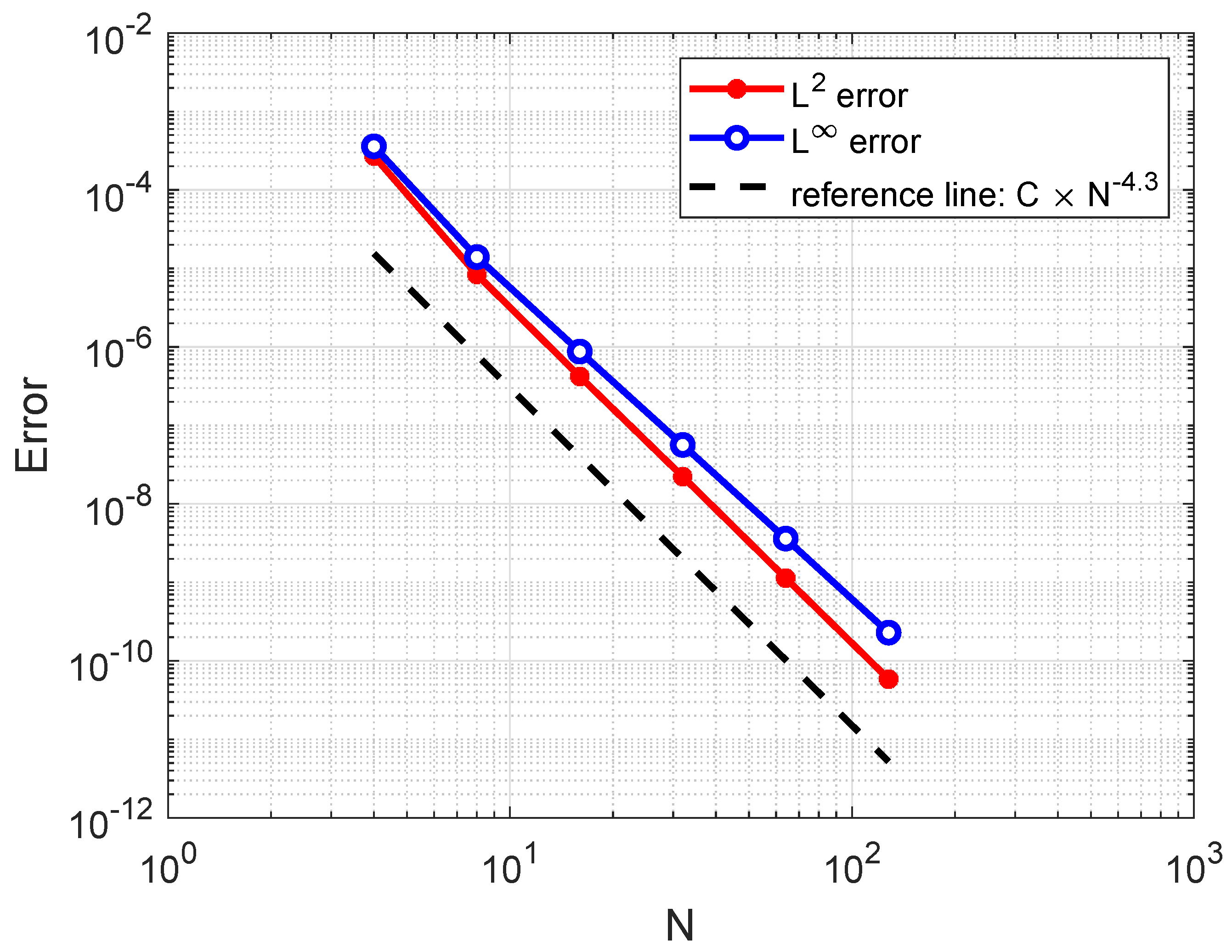
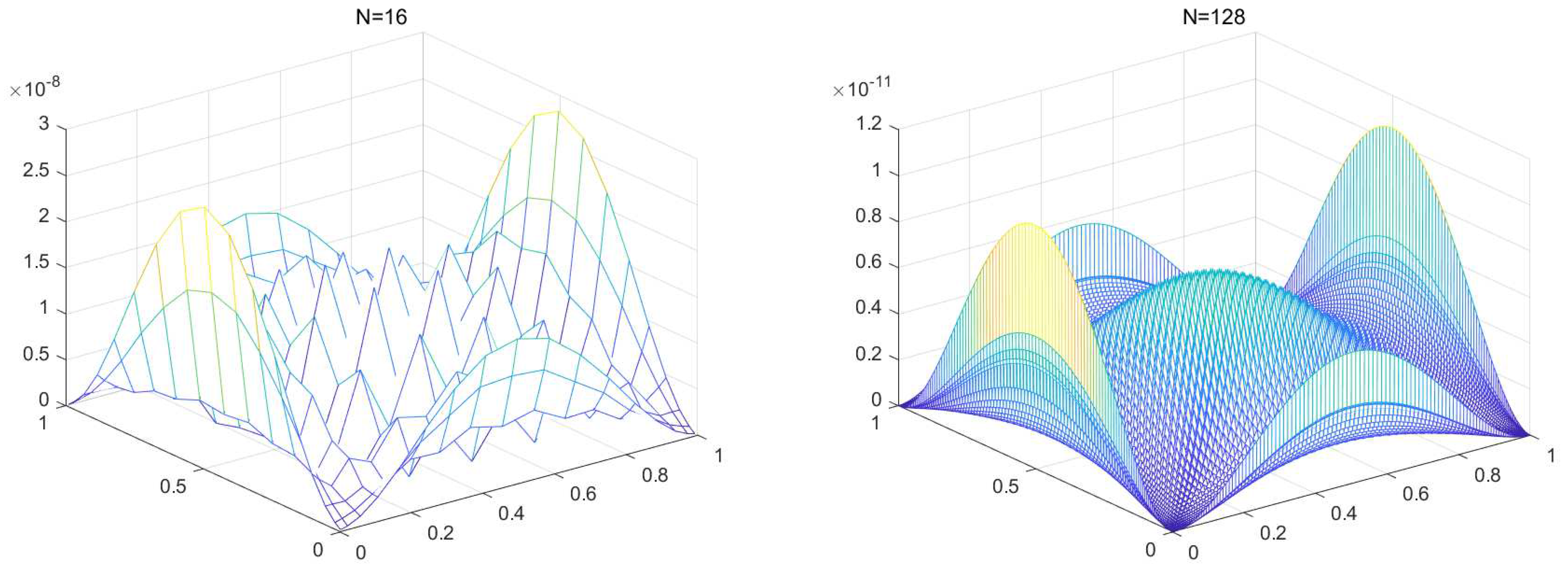
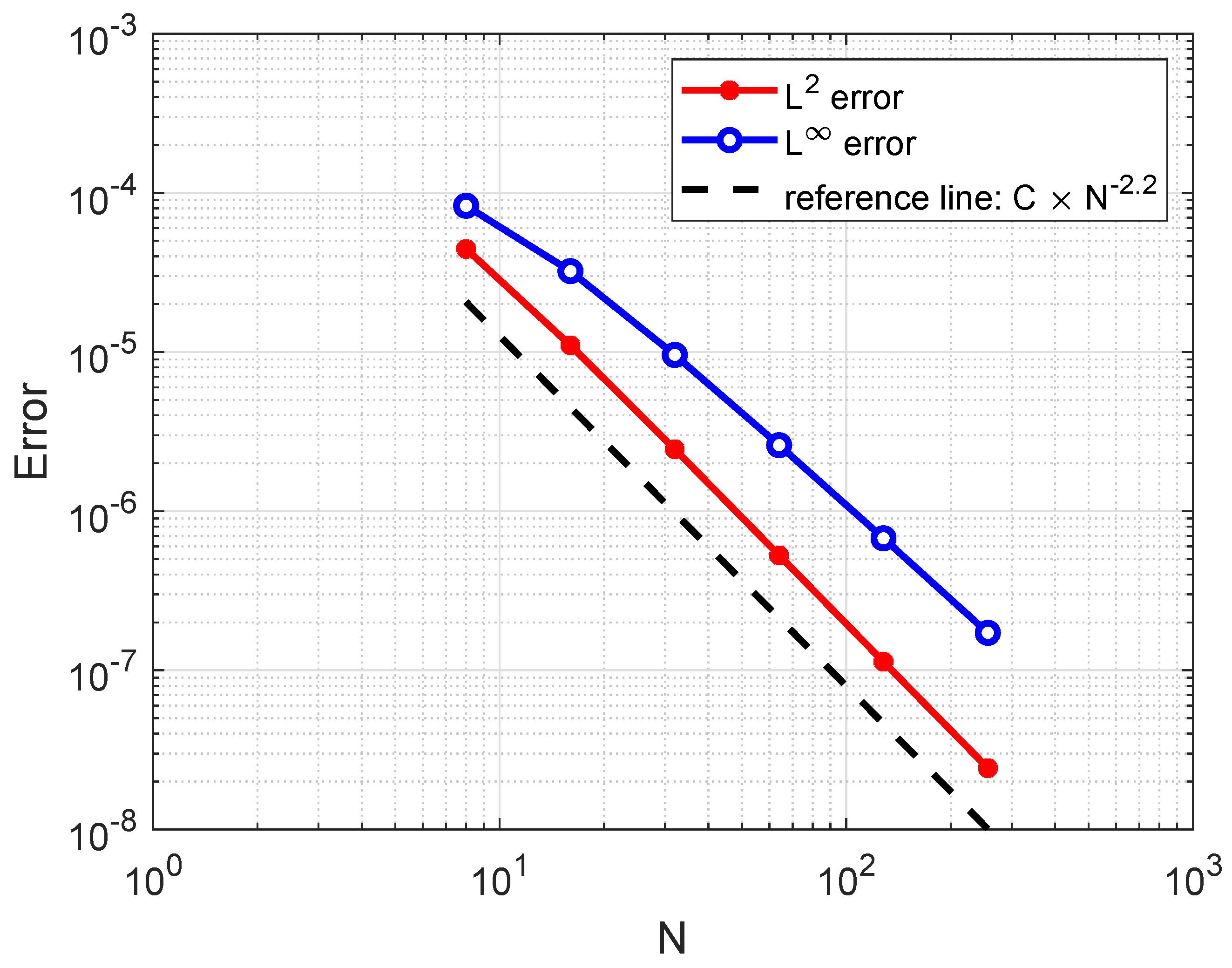
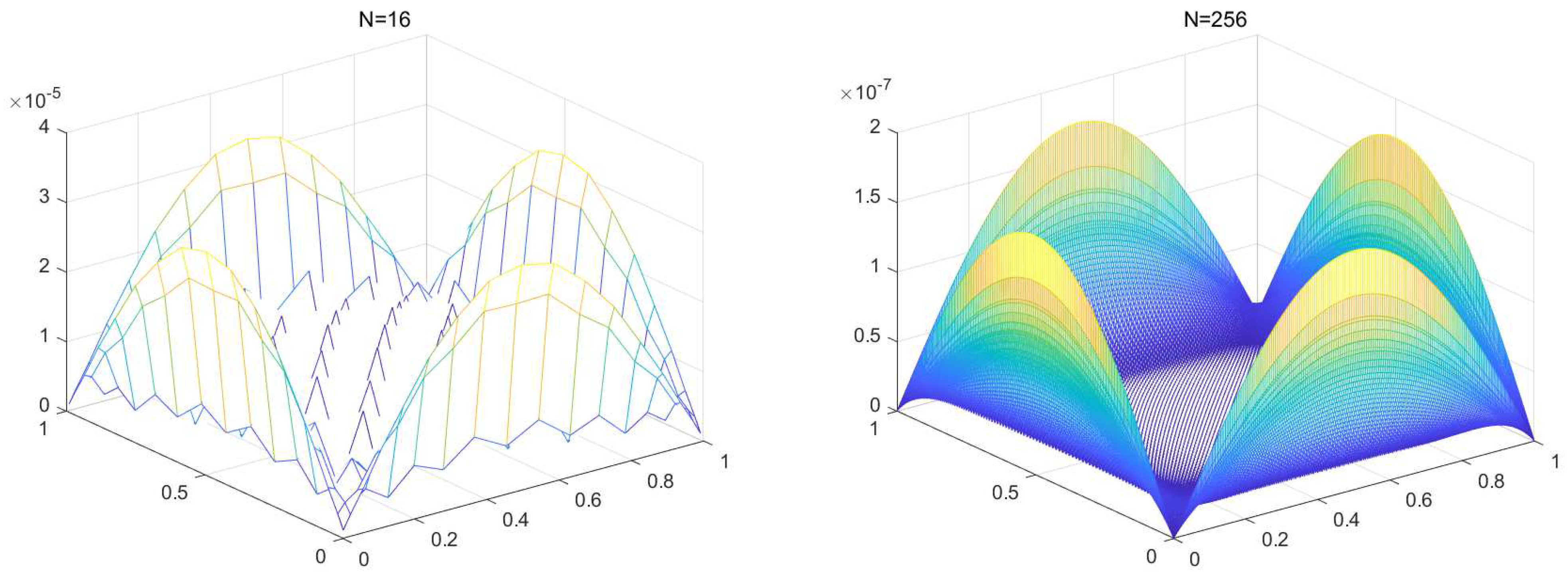
The time step is chosen to be $\tau ={10}^{-4}$ to reduce the impact of the error in the time direction in the above numerical simulations. The numerical results for the fixed time step are plotted in Figure 1, Figure 2, Figure 3, Figure 4, Figure 5, Figure 6, Figure 7 and Figure 8. The ${\mathcal{L}}^{\infty }$ and ${\mathcal{L}}^2$ errors between the exact solution and the numerical solution at $T=1$ are plotted in log–log scale for Examples 1–4 in Figure 1, Figure 3, Figure 5, and Figure 7, respectively. We have sketched a reference line in the figures to show the approximate convergence rate. According to these error plots, it is easy to observe that as the number of nodes increases, the errors decrease rapidly, which is consistent with the conclusion of our error analysis. We picture the absolute values of the error point by point for both time and space intervals for Examples 1 and 2 at $N=16$ in Figure 2 and Figure 4, respectively. For the two-dimensional problems, we have drawn the point-wise error plot at $T=1$ by taking $N=16$ and $N=128$ for Example 3 in Figure 6 and taking $N=16$ and $N=256$ for Example 4 in Figure 8. It can be observed that the point-wise error estimates at the boundary are slightly higher, which is attributed to the singular kernel of the fractional-order differential operator.

Figure 1. The ${\mathcal{L}}^{\infty }$ and ${\mathcal{L}}^2$ errors at $T=1$ for Example 1 when $K_1=K_2=1$, $L=1$, $({\alpha }_1,{\alpha }_2)=(0.6,1.8)$, $\mu =1$, $\nu =-1$, $\tau =0.0001$, and $N=[4,8,16,32,46,128]$.

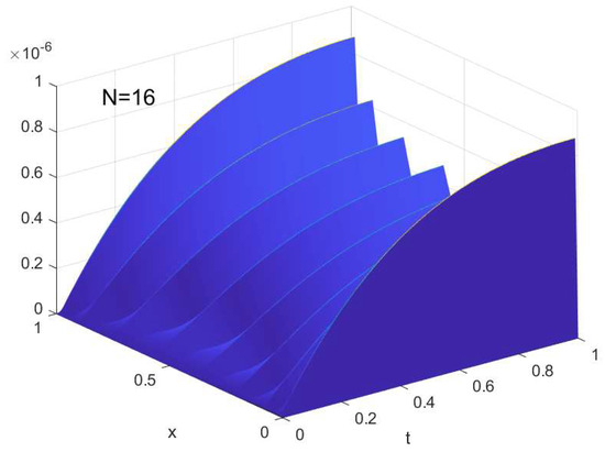
Figure 2. The point-wise error for Example 1 when $K_1=K_2=1$, $L=1$, $({\alpha }_1,{\alpha }_2)=(0.6,1.8)$, $\mu =1$, $\nu =-1$, $\tau =0.0001$, and $N=16$.

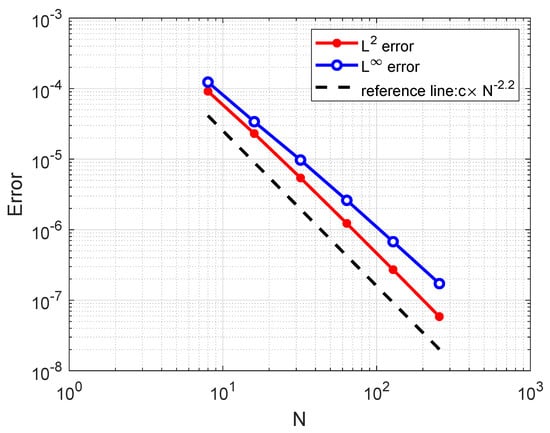
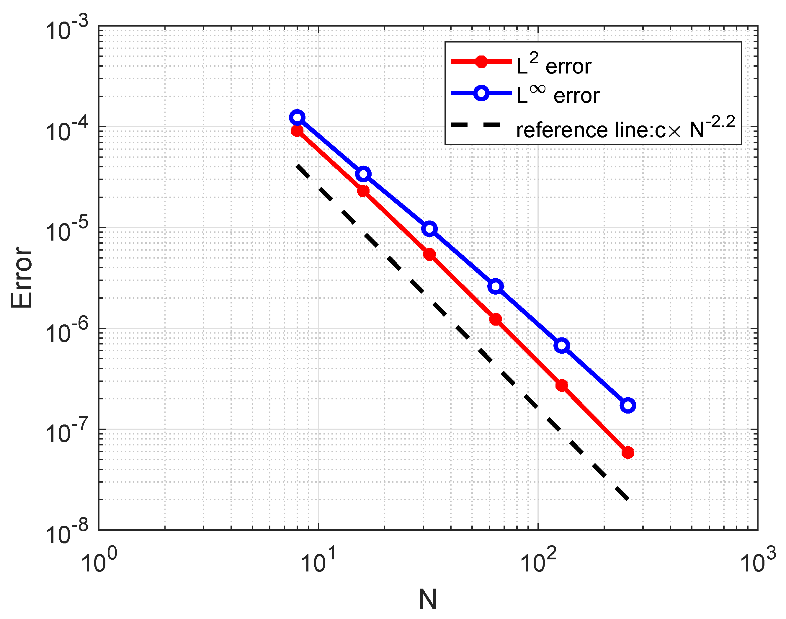
Figure 3. The ${\mathcal{L}}^{\infty }$ and ${\mathcal{L}}^2$ errors at $T=1$ for Example 2 when $K_1=K_2=1$, $L=1$, $({\alpha }_1,{\alpha }_2)=(0.6,1.8)$, $\tau =0.0001$, and $N=[8,16,32,46,128,256]$.

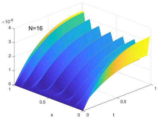
Figure 4. The point-wise error for Example 2 when $K_1=K_2=1$, $L=1$, $({\alpha }_1,{\alpha }_2)=(0.6,1.8)$, $\tau =0.0001$, and $N=16$.

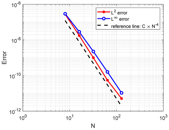
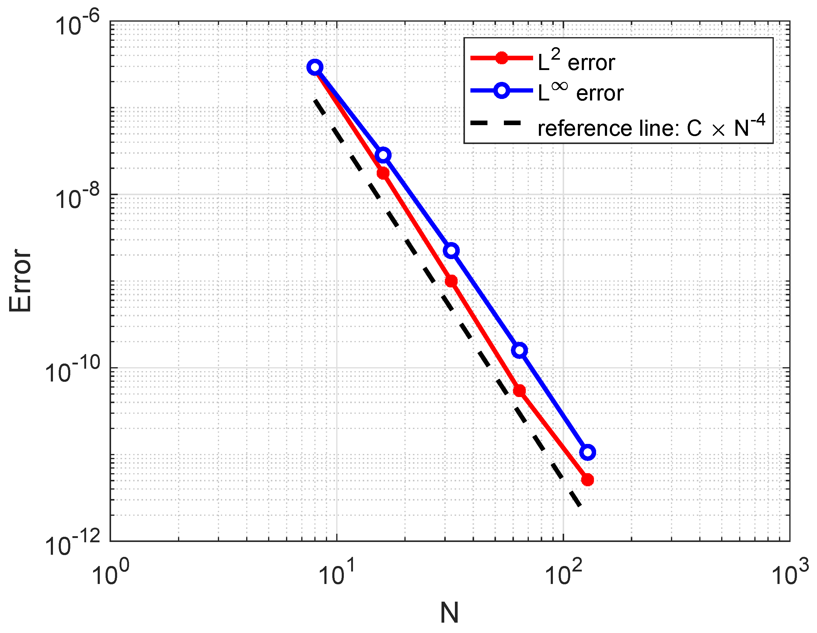
Figure 5. The ${\mathcal{L}}^{\infty }$ and ${\mathcal{L}}^2$ errors at $T=1$ for Example 3 when $K_1=K_2=K_3=K_4=1$, $L=1$, $({\alpha }_1,{\alpha }_2)=(0.6,1.6)$, $({\beta }_1,{\beta }_2)=(0.6,1.8)$, $\tau =0.0001$, and $N=[8,16,32,46,128]$.

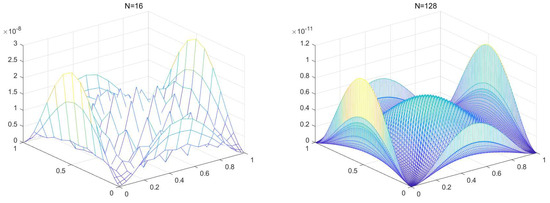
Figure 6. The point-wise error at $T=1$ for Example 3 when $K_1=K_2=K_3=K_4=1$, $L=1$, $({\alpha }_1,{\alpha }_2)=(0.6,1.6)$, $({\beta }_1,{\beta }_2)=(0.6,1.8)$, and $\tau =0.0001$. (Left): $N=16$; (Right): $N=128$.

Figure 7. The ${\mathcal{L}}^{\infty }$ and ${\mathcal{L}}^2$ errors at $T=1$ for Example 4 when $K_1=K_2=K_3=K_4=1$, $L=1$, $({\alpha }_1,{\alpha }_2)=(0.2,1.8)$, $({\beta }_1,{\beta }_2)=(0.6,1.8)$, $\tau =0.0001$, and $N=[8,16,32,46,128,256]$.

Figure 8. The point-wise error at $T=1$ for Example 4 when $K_1=K_2=K_3=K_4$, $L=1$, $({\alpha }_1,{\alpha }_2)=(0.2,1.8)$, $({\beta }_1,{\beta }_2)=(0.6,1.8)$, and $\tau =0.0001$. (Left): $N=16$; (Right): $N=256$.

In the following, we will provide the results of numerical comparison experiments for Example 1 with the finite difference method proposed in [37]. For this analysis, the time step in the simulations is chosen to be $1/N$. The experimental results are listed in Table 1 and Table 2. From the data in the tables, one can see that our proposed method has higher accuracy and generally results in higher convergence orders. This is due to the spectral methods used in the spatial domain, which has spectral accuracy for smooth functions. The reason that the convergence order is much lower than that shown in Figure 1 is that our method results in a convergence rate of $O\left({\tau }^2\right)$ in the time domain, which holds the total convergence rate back.

Table 1. Convergence order and maximum error for Example 1, which is convection-dominant at $T=1$ when $\nu ={\alpha }_1$, $\mu ={\alpha }_2$, $K_1=2$, and $K_2=0.25$.

		${\mathit{\alpha }}_1=0.1$		${\mathit{\alpha }}_1=0.45$		${\mathit{\alpha }}_1=0.85$
	$\mathit{N}(\mathbf{1}/\mathit{\tau })$	${\mathbf{err}}_{{\mathcal{L}}^{\infty }}{|}_{\mathit{t}=\mathbf{1}}$	Order	${\mathbf{err}}_{{\mathcal{L}}^{\infty }}{|}_{\mathit{t}=\mathbf{1}}$	Order	${\mathbf{err}}_{{\mathcal{L}}^{\infty }}{|}_{\mathit{t}=\mathbf{1}}$	Order
	10	$1.7575\times {10}^{-4}$	−	$7.6952\times {10}^{-4}$	−	$2.3088\times {10}^{-3}$	−
	20	$3.3515\times {10}^{-5}$	$2.3906$	$1.7774\times {10}^{-4}$	$2.1142$	$5.3559\times {10}^{-4}$	$2.1080$
${\alpha }_2=1.25$	40	$5.1936\times {10}^{-6}$	$2.6900$	$4.2000\times {10}^{-5}$	$2.0813$	$1.2951\times {10}^{-4}$	$2.0481$
	80	$1.0632\times {10}^{-6}$	$2.2883$	$9.6456\times {10}^{-6}$	$2.1224$	$3.1667\times {10}^{-5}$	$2.0320$
	160	$6.5589\times {10}^{-7}$	$0.6969$	$2.0735\times {10}^{-6}$	$2.2178$	$7.7614\times {10}^{-6}$	$2.0286$
	10	$6.6256\times {10}^{-4}$	−	$1.6599\times {10}^{-3}$	−	$4.0506\times {10}^{-3}$	−
	20	$1.6206\times {10}^{-4}$	$2.0316$	$3.9472\times {10}^{-4}$	$2.0722$	$9.3815\times {10}^{-4}$	$2.1103$
${\alpha }_2=1.85$	40	$4.0207\times {10}^{-5}$	$2.0110$	$9.6426\times {10}^{-5}$	$2.0333$	$2.2591\times {10}^{-4}$	$2.0541$
	80	$9.9963\times {10}^{-6}$	$2.0080$	$2.3816\times {10}^{-5}$	$2.0175$	$5.5400\times {10}^{-5}$	$2.0278$
	160	$2.4873\times {10}^{-6}$	$2.0068$	$5.9151\times {10}^{-6}$	$2.0094$	$1.3715\times {10}^{-5}$	$2.0141$

Table 2. Convergence order and maximum error for Example 1, which is diffusion-dominant at $T=1$ when $\nu ={\alpha }_1$, $\mu ={\alpha }_2$, $K_1=0.25$, and $K_2=2$.

		${\mathit{\alpha }}_1=0.1$		${\mathit{\alpha }}_1=0.45$		${\mathit{\alpha }}_1=0.85$
	$\mathit{N}(\mathbf{1}/\mathit{\tau })$	${\mathbf{err}}_{{\mathcal{L}}^{\infty }}{|}_{\mathit{t}=\mathbf{1}}$	Order	${\mathbf{err}}_{{\mathcal{L}}^{\infty }}{|}_{\mathit{t}=\mathbf{1}}$	Order	${\mathbf{err}}_{{\mathcal{L}}^{\infty }}{|}_{\mathit{t}=\mathbf{1}}$	Order
	10	$2.1908\times {10}^{-4}$	−	$8.4270\times {10}^{-4}$	−	$2.4135\times {10}^{-3}$	−
	20	$4.9719\times {10}^{-5}$	$2.1396$	$1.9674\times {10}^{-4}$	$2.0987$	$5.5850\times {10}^{-4}$	$2.1115$
${\alpha }_2=1.25$	40	$1.2464\times {10}^{-5}$	$1.9960$	$4.8421\times {10}^{-5}$	$2.0226$	$1.3554\times {10}^{-4}$	$2.0428$
	80	$3.0933\times {10}^{-6}$	$2.0106$	$1.1983\times {10}^{-5}$	$2.0146$	$3.3352\times {10}^{-5}$	$2.0229$
	160	$7.6035\times {10}^{-7}$	$2.0244$	$2.9711\times {10}^{-6}$	$2.0119$	$8.2632\times {10}^{-6}$	$2.0130$
	10	$7.2807\times {10}^{-4}$	−	$1.8363\times {10}^{-3}$	−	$4.4266\times {10}^{-3}$	−
	20	$1.6902\times {10}^{-4}$	$2.1069$	$4.2649\times {10}^{-4}$	$2.1063$	$1.0152\times {10}^{-3}$	$2.1244$
${\alpha }_2=1.85$	40	$4.2081\times {10}^{-5}$	$2.0059$	$1.0427\times {10}^{-4}$	$2.0322$	$2.4453\times {10}^{-4}$	$2.0537$
	80	$1.0500\times {10}^{-5}$	$2.0028$	$2.5777\times {10}^{-5}$	$2.0162$	$5.9981\times {10}^{-5}$	$2.0274$
	160	$2.6225\times {10}^{-6}$	$2.0014$	$6.4080\times {10}^{-6}$	$2.0081$	$1.4852\times {10}^{-5}$	$2.0139$

6. Conclusions

In this paper, we studied spectral Galerkin methods for the one-dimensional and two-dimensional Riesz space-fractional convection–diffusion equations in (1).

Firstly, we developed the semi-discrete and fully discrete schemes of the one-dimensional equation in (2) using the CNLF scheme for discretization in the temporal direction and the spectral Galerkin–Legendre method for discretization in the spatial direction. We then rewrote the fully discrete form into a matrix-vector form, as in (8), and provided detailed calculation formulas for all matrices. Subsequently, we meticulously proved the theorems of stability and convergence for the semi-discrete and fully discrete schemes and showed that the schemes are stable with a convergence order of $O({\tau }^2+N^{{\alpha }_1/2-r}+N^{{\alpha }_2/2-r})$, where $\tau$ is the time step, $N+1$ is the number of spatial nodes, ${\alpha }_1$ and ${\alpha }_2$ are the orders of fractional derivatives, and r represents the smoothness of the function.

Secondly, we established the fully discrete format for two-dimensional problems, as in (23), in a similar way. We added a supplementary term ${\tau }^2{F}_x{F}_y{\delta }_{\hat{t}}{u}^n$ to the left side of Equation (26), resulting in a symmetric fully discrete scheme. Next, we transformed the fully discrete form into a matrix-vector form, as in (31). Stability and convergence analyses of the semi-discrete and fully discrete schemes for two-dimensional problems were then presented, and the conclusions obtained were consistent with the one-dimensional case.

Finally, several numerical examples were designed, and the simulation results verified our theoretical study and analysis of our proposed numerical methods.

From the analysis and numerical results, we can see that the convergence rate in the temporal direction hinders the fast convergence rate in the spatial direction. In the future, we will study algorithms that apply spectral methods to both the time and space domains.

References

- Saichev, A.I.; Zaslavsky, G.M. Fractional Kinetic Equations: Solutions and Applications. Chaos Interdiscip. J. Nonlinear Sci. 1997, 7, 753–764. [Google Scholar] [CrossRef] [PubMed]
- Mandelbrot, B.B.; Mandelbrot, B.B. The Fractal Geometry of Nature; WH Freeman: New York, NY, USA, 1982; pp. 54–96. [Google Scholar]
- Mainardi, F. Some Basic Problem in Continum and Statistical Mechanics. Fractals Fract. Calc. Contin. Mech. 1997, 378, 291–348. [Google Scholar]
- Bagley, R.L.; Torvik, P.J. A Theoretical Basis for the Application of Fractional Calculus to Viscoelasticity. J. Rheol. 1983, 27, 201–210. [Google Scholar] [CrossRef]
- Bagley, R.L.; Torvik, P.J. Fractional Calculus in the Transient Analysis of Viscoelastically Damped Structures. AIAA J. 1985, 23, 918–925. [Google Scholar] [CrossRef]
- Hilfer, R. Applications of Fractional Calculus in Physics; World Scientific: Singapore, 2000; pp. 10–25. [Google Scholar]
- Scalas, E.; Gorenflo, R.; Mainardi, F. Fractional Calculus and Continuous-Time Finance. Phys. A Stat. Mech. Its Appl. 2000, 284, 376–384. [Google Scholar] [CrossRef]
- Mainardi, F.; Raberto, M.; Gorenflo, R.; Scalas, E. Fractional Calculus and Continuous-Time Finance II: The Waiting-Time Distribution. Phys. A Stat. Mech. Its Appl. 2000, 287, 468–481. [Google Scholar] [CrossRef]
- Wang, S.; Xu, M. Generalized Fractional Schrödinger Equation with Space-Time Fractional Derivatives. J. Math. Phys. 2007, 48, 2–10. [Google Scholar] [CrossRef]
- Huang, F.; Liu, F. The Fundamental Solution of the Space-Time Fractional Advection-Dispersion Equation. J. Appl. Math. Comput. 2005, 18, 339–350. [Google Scholar]
- El-Sayed, A.; Behiry, S.; Raslan, W. Adomian’s Decomposition Method for Solving an Intermediate Fractional Advection-Dispersion Equation. Comput. Math. Appl. 2010, 59, 1759–1765. [Google Scholar] [CrossRef]
- Golbabai, A.; Sayevand, K. Analytical Modelling of Fractional Advection-Dispersion Equation Defined in a Bounded Space Domain. Math. Comput. Model. 2010, 53, 1708–1718. [Google Scholar] [CrossRef]
- Canuto, C.; Hussaini, M.Y.; Quarteroni, A.; Zang, T.A. Spectral Methods: Fundamentals in Single Domains; Springer Science & Business Media: Berlin/Heidelberg, Germany, 2007; pp. 20–35. [Google Scholar]
- Santos, M.A.F. Analytic approaches of the anomalous diffusion: A review. Chaos Solitons Fractals 2019, 124, 86–96. [Google Scholar] [CrossRef]
- Benson, D.A.; Wheatcraft, S.W.; Meerschaert, M.M. Application of a Fractional Advection-Dispersion Equation. Water Resour. Res. 2000, 36, 1403–1412. [Google Scholar] [CrossRef]
- Benson, D.A.; Wheatcraft, S.W.; Meerschaert, M.M. The Fractional-Order Governing Equation of Lévy Motion. Water Resour. Res. 2000, 36, 1413–1423. [Google Scholar] [CrossRef]
- Metzler, R.; Klafter, J. The Random Walk’s Guide to Anomalous Diffusion: A Fractional Dynamics Approach. Phys. Rep. 2000, 339, 1–77. [Google Scholar] [CrossRef]
- Metzler, R.; Klafter, J. The Restaurant at the end of the Random Walk: Recent Developments in the Description of Anomalous Transport by Fractional Dynamics. J. Phys. A Math. Gen. 2004, 37, R161. [Google Scholar] [CrossRef]
- Zaslavsky, G.M. Chaos, Fractional Kinetics and Anomalous transport. Phys. Rep. 2002, 371, 461–580. [Google Scholar] [CrossRef]
- Schumer, R.; Benson, D.A.; Meerschaert, M.M.; Wheatcraft, S.W. Eulerian Derivation of the Fractional Advection-Dispersion Equation. J. Contam. Hydrol. 2001, 48, 69–88. [Google Scholar] [CrossRef]
- Sun, Z.; Wu, X. A Fully Discrete Difference Scheme for a Diffusion-Wave System. Appl. Numer. Math. 2006, 56, 193–209. [Google Scholar] [CrossRef]
- Liu, Q.; Liu, F.; Turner, I.; Anh, V. Approximation of the Lévy-Feller Advection-Dispersion Process by Random Walk and Finite Difference Method. J. Comput. Phys. 2007, 222, 57–70. [Google Scholar] [CrossRef]
- Shen, S.; Liu, F.; Anh, V. Numerical Approximations and Solution Techniques for the Space-Time Riesz-Caputo Fractional Advection-Diffusion Equation. Numer. Algorithms 2011, 56, 383–403. [Google Scholar] [CrossRef]
- Zhou, H.; Tian, W.; Deng, W. Quasi-Compact Finite Difference Schemes for Space Fractional Diffusion Equations. J. Sci. Comput. 2013, 56, 45–66. [Google Scholar] [CrossRef]
- Wang, K.; Wang, H. A Fast Characteristic Finite Difference Method for Fractional Advection-Diffusion Equations. Adv. Water Resour. 2011, 34, 810–816. [Google Scholar] [CrossRef]
- Huang, Q.; Huang, G.; Zhan, H. A Finite Element Solution for the Fractional Advection-Dispersion Equation. Adv. Water Resour. 2008, 31, 1578–1589. [Google Scholar] [CrossRef]
- Lai, J.; Liu, F.; Anh, V.V.; Liu, Q. A space-time finite element method for solving linear Riesz space fractional partial differential equations. Numer. Algorithms 2021, 88, 499–520. [Google Scholar] [CrossRef]
- Tang, H.; Xia, J. High-Order Accurate Runge-Kutta (Local) Discontinuous Galerkin Methods for One- and Two-Dimensional Fractional Diffusion Equations. Numer. Math. Theory Methods Appl. 2012, 5, 333–358. [Google Scholar] [CrossRef]
- Bhrawy, A.H. A Jacobi Spectral Collocation Method for Solving Multi-Dimensional Nonlinear Fractional Sub-Diffusion Equations. Numer. Algorithms 2016, 73, 91–113. [Google Scholar] [CrossRef]
- Bhrawy, A.H.; Zaky, M.A.; Van Gorder, R.A. A Space-Time Legendre Spectral Tau Method for the Two-Sided Space-Time Caputo Fractional Diffusion-Wave Equation. Numer. Algorithms 2016, 71, 151–180. [Google Scholar] [CrossRef]
- Saadatmandi, A.; Dehghan, M.; Azizi, M.R. The Sinc-Legendre Collocation Method for a class of Fractional Convection-Diffusion Equations with Variable Coefficients. Commun. Nonlinear Sci. Numer. Simul. 2012, 17, 4125–4136. [Google Scholar] [CrossRef]
- Shen, S.; Liu, F.; Anh, V.; Turner, I. The Fundamental Solution and Numerical Solution of the Riesz Fractional Advection-Dispersion Equation. IMA J. Appl. Math. 2008, 73, 850–872. [Google Scholar] [CrossRef]
- Yang, Q.; Liu, F.; Turner, I. Numerical Methods for Fractional Partial Differential Equations with Riesz Space Fractional Derivatives. Appl. Math. Model. 2010, 34, 200–218. [Google Scholar] [CrossRef]
- Zhang, H.; Liu, F.; Anh, V. Galerkin Finite Element Approximation of Symmetric Space-Fractional Partial Differential Equations. Appl. Math. Comput. 2010, 217, 2534–2545. [Google Scholar] [CrossRef]
- Celik, C.; Duman, M. Crank-Nicolson Method for the Fractional Diffusion Equation with the Riesz Fractional Derivative. J. Comput. Phys. 2012, 231, 1743–1750. [Google Scholar] [CrossRef]
- Zeng, F.; Liu, F.; Li, C.; Burrage, K.; Turner, I.; Anh, V. A Crank-Nicolson ADI Spectral Method for a Two-Dimensional Riesz Space Fractional Nonlinear Reaction-Diffusion Equation. SIAM J. Numer. Anal. 2014, 52, 2599–2622. [Google Scholar] [CrossRef]
- Anley, E.F.; Zheng, Z. Finite Difference Method for Two-Sided Two Dimensional Space Fractional Convection-Diffusion Problem with Source Term. Mathematics 2020, 8, 1878. [Google Scholar] [CrossRef]
- Basha, M.; Anley, E.F.; Dai, B. Linearized Crank–Nicolson Scheme for the Two-Dimensional Nonlinear Riesz Space-Fractional Convection–Diffusion Equation. Fractal Fract. 2023, 7, 240. [Google Scholar] [CrossRef]
- Li, J.; Liu, F.; Feng, L.; Turner, I. A Novel Finite Volume Method for the Riesz Space Distributed-Order Diffusion Equation. Comput. Math. Appl. 2017, 74, 772–783. [Google Scholar] [CrossRef]
- Li, J.; Liu, F.; Feng, L.; Turner, I. A Novel Finite Volume Method for the Riesz Space Distributed-Order Advection-Diffusion Equation. Appl. Math. Model. 2017, 46, 536–553. [Google Scholar] [CrossRef]
- Ye, H.; Liu, F.; Anh, V.; Turner, I. Numerical Analysis for the Time Distributed-Order and Riesz Space Fractional Diffusions on Bounded Domains. IMA J. Appl. Math. 2015, 80, 825–838. [Google Scholar] [CrossRef]
- Zhang, H.; Liu, F.; Jiang, X.; Zeng, F.; Turner, I. A Crank-Nicolson ADI Galerkin-Legendre Spectral Method for the Two-Dimensional Riesz Space Distributed-Order Advection-Diffusion Equation. Comput. Math. Appl. 2018, 76, 2460–2476. [Google Scholar] [CrossRef]
- Hu, X.; Liu, F.; Turner, I.; Anh, V. An Implicit Numerical Method of a New Time Distributed-Order and Two-Sided Space-Fractional Advection-Dispersion Equation. Numer. Algorithms 2016, 72, 393–407. [Google Scholar] [CrossRef]
- Ding, H.; Zhang, Y. New numerical methods for the Riesz space fractional partial differential equations. Comput. Math. Appl. 2012, 63, 1135–1146. [Google Scholar]
- Shen, J.; Tang, T.; Wang, L. Spectral Methods: Algorithms, Analysis and Applications; Springer Science & Business Media: Berlin/Heidelberg, Germany, 2011. [Google Scholar]
- Ervin, V.J.; Roop, J.P. Variational solution of fractional advection dispersion equations on bounded domains in Rd. Numer. Methods Partial. Differ. Equ. Int. J. 2007, 23, 256–281. [Google Scholar] [CrossRef]
- Bærentzen, J.A.; Gravesen, J.; Anton, F.; Aanæs, H. Finite Difference Methods for Partial Differential Equations. In Guide to Computational Geometry Processing; Springer: London, UK, 2012; pp. 65–79. [Google Scholar]
Disclaimer/Publisher’s Note: The statements, opinions and data contained in all publications are solely those of the individual author(s) and contributor(s) and not of MDPI and/or the editor(s). MDPI and/or the editor(s) disclaim responsibility for any injury to people or property resulting from any ideas, methods, instructions or products referred to in the content. |
© 2024 by the authors. Licensee MDPI, Basel, Switzerland. This article is an open access article distributed under the terms and conditions of the Creative Commons Attribution (CC BY) license (https://creativecommons.org/licenses/by/4.0/).