FLRNN-FGA: Fractional-Order Lipschitz Recurrent Neural Network with Frequency-Domain Gated Attention Mechanism for Time Series Forecasting

Abstract

Time series forecasting has played an important role in different industries, including economics, energy, weather, and healthcare. RNN-based methods have shown promising potential due to their strong ability to model the interaction of time and variables. However, they are prone to gradient issues like gradient explosion and vanishing gradients. And the prediction accuracy is not high. To address the above issues, this paper proposes a Fractional-order Lipschitz Recurrent Neural Network with a Frequency-domain Gated Attention mechanism (FLRNN-FGA). There are three major components: the Fractional-order Lipschitz Recurrent Neural Network (FLRNN), frequency module, and gated attention mechanism. In the FLRNN, fractional-order integration is employed to describe the dynamic systems accurately. It can capture long-term dependencies and improve prediction accuracy. Lipschitz weight matrices are applied to alleviate the gradient issues. In the frequency module, temporal data are transformed into the frequency domain by Fourier transform. Frequency domain processing can reduce the computational complexity of the model. In the gated attention mechanism, the gated structure can regulate attention information transmission to reduce the number of model parameters. Extensive experimental results on five real-world benchmark datasets demonstrate the effectiveness of FLRNN-FGA compared with the state-of-the-art methods.

1. Introduction

Time series data play an important role in modern society [1,2,3]. A large number of time series data are presented in various fields, such as finance [4], economics [5], transportation [6], and meteorology [7]. These time series data contain a wealth of useful information. Accurate analysis and information extraction can help decision makers and managers in various fields to mitigate risks, manage resources, predict future trends, and formulate long-term plans for better development.

Traditional time series forecasting methods are mainly divided into statistical methods and grey models [8,9]. These methods can achieve good forecasting results for low-dimensional and stationary time series data [10]. However, accurately forecasting high-dimensional and non-stationary time series data remains challenging. For forecasting complex time series data, deep learning technology, with its powerful computational and learning capabilities, has become a research hotspot in the academic community [9,10]. Compared to statistical time series forecasting models, deep learning models can handle complex nonlinear relationships. Additionally, deep learning models can accurately capture the long-term dependencies in sequences [11,12].

Recently, thanks to their tremendous success in natural language processing and computer vision [13,14], Transformers have also been successfully applied to time series tasks, with a great many Transformer variants being proposed [15]. This is attributed to the attention mechanism’s ability to enhance the model’s focus and understanding of different parts of the time series, allowing it to more effectively learn and utilize the information in the time series, thereby improving prediction accuracy. However, Transformer modeling requires substantial computational resources and costs, which limits its development in time series forecasting [16,17,18]. To this end, in this paper, we adopt recurrent neural networks as the main structure.

The recurrent neural network (RNN) model can establish temporal dependencies through recursion, and it is considered suitable for handling sequential data [19]. Many studies have indicated the effectiveness of recurrent neural network models in time series data [20]. However, when recurrent neural network models are applied to long-sequence tasks, they are prone to gradient issues like gradient explosion and vanishing gradients [21,22]. Although long short-term memory (LSTM) networks and other variants alleviate these issues to some extent, there still exist problems with inaccurate dynamic descriptions and high computational complexity.

In order to address these gradient-related issues, Hochreiter proposed the long short-term memory (LSTM) networks [23]. The LSTM networks use gate structures to control the flow of gradients to solve gradient-related issues. Benefiting from the dynamic systems perspective of RNNs [24,25,26], Rubanova and Brouwer formulated new recurrent model equations and their discrete integrals based on differential theory [27]. Lechner and Hasani extended these models based on ordinary differential equations [28]. They designed an ordinary differential equation model based on the LSTM to address the gradient vanishing and exploding issues. Ding combined fuzzy systems to construct the recurrent fuzzy neural network [29]. Park applied a dual RNN architecture with partial linear dependencies to forecast time series data [30]. Erichson reconstructed the weight matrices of recurrent units using Lipschitz RNN to alleviate the gradient issues [31]. However, the prediction accuracy was not high.

For the prediction accuracy, fractional calculus theory can achieve more accurate predictions because fractional calculus is an expansion of integer calculus, which can more accurately describe the actual system. And fractional-order systems have more precise results [32]. The essence of the world is a fractional-order system. And numerous natural phenomena cannot be precisely captured by traditional integer-order calculus equations. Therefore, an extension of traditional calculus is necessary to better describe and analyze such occurrences. Using Lipschitz recurrent units, the issues of gradient vanishing and exploding in recurrent neural networks for long-term sequence prediction tasks are alleviated.

To overcome the above problems, this paper proposes a Fractional-order Lipschitz Recurrent Neural Network with a Frequency-domain Gated Attention mechanism (FLRNN-FGA) for time series prediction. Deep learning techniques and fractional calculus theory can achieve more accurate predictions of long-term time series data by capturing the long-term dependencies of the time series. This paper utilizes piecewise recurrent units, which can effectively reduce the number of iterations of the recurrent units. Based on fractional calculus, fractional-order integration is used to accurately describe the dynamics of the system [33], and it can enhance the model’s ability to capture long-term dependencies and improve the prediction accuracy. By introducing Fourier transform, the temporal data are transformed into the frequency domain. Some processing is conducted, including frequency domain selection and sampling. This reduces the computational complexity of the model, addressing the inefficiency involved in handling long-term time series data. To address the issue of insufficient feature interaction in the model, a gated attention mechanism is adopted, which combines gated techniques with an attention mechanism. The gated structure can adjust the information flow of the attention, enabling the model to filter out noise and avoid its introduction. This facilitates better handling of inter-variable relationships, enhancing features while reducing model parameter count and improving efficiency. The main contributions of this study are as follows.

• A new Fractional-order Lipschitz Recurrent Neural Network with a Frequency-domain Gated Attention mechanism is proposed for time series prediction. Extensive experimental results on five datasets demonstrate the effectiveness of this method.
• This paper introduces fractional calculus to describe the system dynamics of recurrent neural networks, effectively improving the model’s prediction accuracy.
• In this paper, piecewise recurrent units are introduced to reduce the number of iterations of recurrent units. By reconstructing the weight matrix of the recurrent layer to control the system’s dynamic changes, the gradient problem in recurrent neural networks is effectively alleviated.
• This paper combines gated techniques with an attention mechanism to regulate attention information, which can reduce the number of model parameters and effectively improve the model’s efficiency and accuracy.

The remainder of the article is structured in the following way. In Section 3, the FLRNN-FGA method is deduced in detail. Section 4 verifies the effectiveness of the proposed method through some experiments. Finally, our conclusions are derived in Section 5.

2. Related Work

A Time Series Forecasting Model Based on RNNs

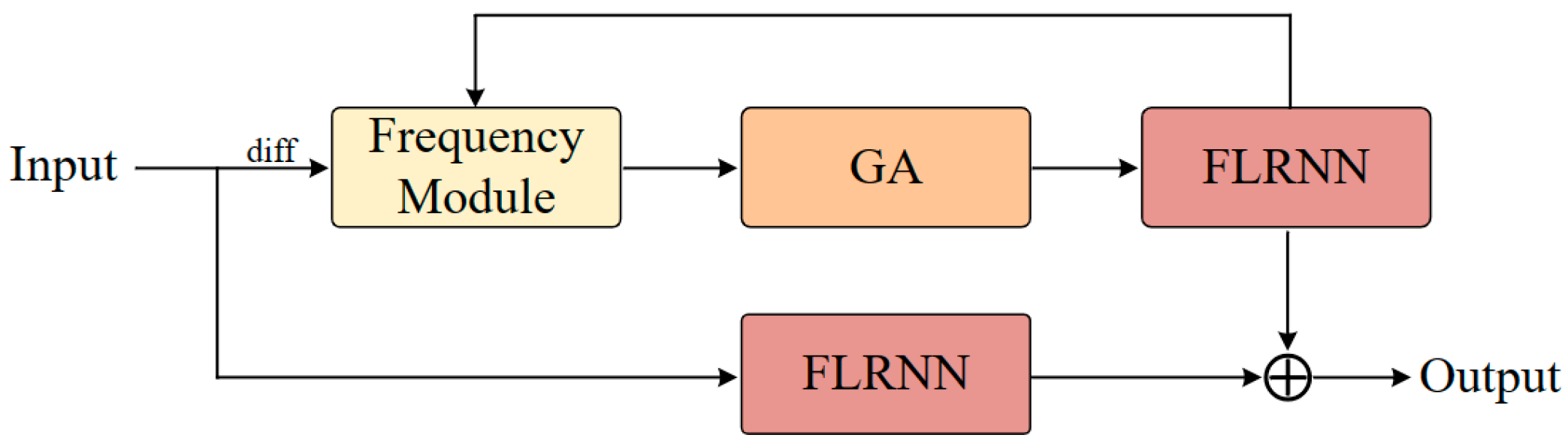
Recurrent neural networks (RNNs) have long been the preferred choice for time series forecasting tasks due to their ability to handle sequential data. Extensive research has focused on applying RNNs to short-term and probabilistic forecasting, achieving significant progress. For instance, the work by Lai et al. [33], Wen et al. [34], Tan, Xie, and Cheng [35], and Bergsma et al. [36] has made important contributions in this area. However, in the field of long-term sequence forecasting (LTSF), RNNs are considered ineffective at capturing long-term dependencies when faced with excessively long historical windows and prediction horizons, leading to their gradual abandonment [37,38].

To address these challenges, novel RNN architectures such as SegRNN and RWKV-TS have emerged, aiming to enhance the ability of RNNs to capture long-term dependencies by improving their structure. Additionally, in the field of large-scale language models, some new RNN architectures, like RWKV, Retentive Network [39], and Mamba [40], have demonstrated performance comparable to Transformer models [41], while also being more efficient. These new developments suggest that, despite the limitations of traditional RNNs in certain long-sequence forecasting tasks, RNNs still hold great potential in time series forecasting through architectural innovation and improvement.

However, when recurrent neural network (RNN) models are applied to long-sequence tasks, they are prone to issues such as gradient explosion and gradient vanishing. Although long short-term memory (LSTM) networks and other variants have mitigated these issues to some extent, they still face challenges related to inaccurate dynamic descriptions and high computational complexity.

3. Methods

Addressing the issues of inaccurate prediction and gradient problems in recurrent neural networks, a Fractional-order Lipschitz Recurrent Neural Network with a Frequency-domain Gated Attention mechanism (FLRNN-FGA) is proposed for time series prediction. The model architecture of FLRNN-FGA is depicted in Figure 1, which mainly involves the Fractional-order Lipschitz Recurrent Neural Network (FLRNN), frequency module, and gated attention mechanism.

First, we present our redesigned FLRNN architecture of FLRNN-FGA in Section 3.1 Time Series Forecasting Model Based on RNN. Here, piecewise recurrent units are introduced. The segmented sequence is used as the input to the Lipschitz recurrent unit. Through segmented recurrent units, the model can accelerate the processing speed of the recurrent units for long sequences without compromising their performance. By employing fractional-order Lipschitz recurrent units, it is possible to control the sensitivity of the system. And it can alleviate gradient issues and accurately capture system dynamics and dependencies. Thus, more precise predictions can be provided for time series tasks. Then, we present the frequency module in Section 3.2. The temporal data are transformed into the frequency domain by Fourier transform. Then, the low-frequency part that contains more sequence information is selected using frequency domain selection. A strategy of random frequency domain sampling is employed to reduce the computational overhead. Frequency domain processing can effectively decrease the computational cost while retaining crucial sequence features. In addition, we also present the detailed gated attention mechanism in Section 3.3. This combines gated techniques with an attention mechanism. The correlation between features is captured by attention. Then, it can be enhanced through feature interaction. The gated structure can regulate the attention information transmission. That method can reduce the number of model parameters.

3.1. FLRNN

The Fractional-order Lipschitz Recurrent Neural Network (FLRNN) can achieve a more accurate result and avoid gradient vanishing and exploding problems.

The recurrent neural network is shown as follows.

$$\left\{\begin{array}{l}\dot{h}=A_{{\beta }_A,{\gamma }_A}h+\tanh \left(W_{{\beta }_W,{\gamma }_W}h+Ux+b\right)\\ y=Dh\end{array}\right.$$

(1)

where $h$ represents the hidden state that contains past information. $\dot{h}$ is the derivative of the hidden state h with respect to time. $A$, $W,$ and $U$ are matrices. $b$ is the offset of the system. x is input, and $y$ is output. The Lipschitz Recurrent Neural Network reconstructed the hidden layer weight matrix [22] as follows.

$$\left\{\begin{array}{cc}{A}_{{\beta }_A,{\gamma }_A}& =\left(1-{\beta }_A\right)\left(M_A+M_A^T\right)+{\beta }_A\left(M_A-M_A^T\right)-{\gamma }_{A}I\\ W_{{\beta }_W,{\gamma }_W}& =\left(1-{\beta }_W\right)\left(M_W+M_W^T\right)+{\beta }_W\left(M_W-M_W^T\right)-{\gamma }_{W}I\end{array}\right.$$

(2)

where $I$ is a unit diagonal matrix. $M_A^T$ and $M_W^T$ are transposed matrices. $\beta \mathrm{ }$ and $\mathrm{ }\gamma \mathrm{ }$ are used to control the spectrum of the weight matrix. The former one controls the width of the spectrum, and the latter one shifts the position of the entire spectrum. The Lipschitz Recurrent Neural Network obtains the hidden state $h$ through numerical integration.

$$h=\Delta t\sum \dot{h}\left(t-r\Delta t\right)$$

(3)

To describe the system dynamics more accurately, fractional-order GL calculus [42] can be used to compute this hidden state. Fractional calculus is a generalization of classical calculus where the order of differentiation and integration can be a fraction rather than an integer. This generalization allows the modeling of systems with memory and hereditary properties, which are common in real-world phenomena. In the FLRNN, fractional calculus is used to integrate the hidden states of the RNN.

$${}_{a}D_t^{\alpha } f(t)=\underset{\mathrm{p}\to 0}{{\displaystyle \lim }}{p}^{-\alpha }{\displaystyle \sum _{j=0}^{\left[(t-a)/p\right]}{(-1)}^j\left(\begin{array}{l}\alpha \\ j\end{array}\right)}f(t-jp)$$

(4)

where $f$ is the function, and $\mathrm{p}$ i0s the step. $\alpha$ represents the fractional order. And $\left(\begin{array}{l}\alpha \\ j\end{array}\right)$ expresses a binomial coefficient, and j denotes a natural number.

Here, fractional-order integration is employed to calculate the hidden state of the system.$\dot{ h }$is taken as the integrand. The coefficient ${\left(-1\right)}^j\left({\displaystyle \genfrac{}{}{0pt}{}{\alpha }{j}}\right)$ can be pre-computed before training. The hidden state $h$ can be computed through fractional-order integration, and it is shown in Equation (5).

$$D_t^{-p}\left(h\left(t\right)\right)=\Delta t^p\sum 〈\begin{array}{c}p\\ r\end{array}〉h\left(t-r\Delta t\right)$$

(5)

where $D_t^{-p}$is a p-order integration operator, and it can be a non-integer. The $<\cdot >$ represents the Grünwald number. Its computation process is shown in Equation (6).

$$〈\begin{array}{c}p\\ r\end{array}〉={\displaystyle \frac{p\left(p+1\right)\cdots \left(p+r+1\right)}{r!}}={\left(-1\right)}^r\left(\begin{array}{c}-p\\ r\end{array}\right)$$

(6)

Fractional calculus is a generalization of integer-order calculus, where the order is not limited to integers but can be any real number or even a complex number. Fractional calculus possesses non-local properties, which are inherent in many complex systems. The dynamic behavior of complex systems can be better described by fractional calculus.

By introducing fractional calculus and Lipschitz recurrent units, this paper constructs a Fractional-order Lipschitz Recurrent Neural Network. And this can accurately capture the temporal relationships in long-term sequential data and alleviate the gradient issue of recurrent neural networks.

Figure 2 shows the structure of the Fractional-order Lipschitz Recurrent Neural Network in this paper, where $x_i$ represents the input data at different time points. ${\mathrm{h}}_0$ represents the initial hidden state of the Lipschitz recurrent unit, and ${\mathrm{h}}_{\mathrm{i}}$ represents the time derivative of the hidden state at different time points, which is calculated through the Lipschitz recurrent unit. After the model calculates the time derivatives at all time points, the final hidden state $h$ is computed through the fractional-order GL integration. Through fractional-order integration, the dynamic behavior of complex systems can be described more accurately, which can make the prediction results more precise.

When recurrent neural networks process sequential data, they typically take the data at a single time point as the input for each iteration. However, adjacent time point data often contain similar information in temporal data analysis. To reduce the training time of the network, this paper proposes that adjacent data segments can be input into the recurrent unit. This approach not only accelerates the training process of the network but also maintains the prediction accuracy of the model. The structure of the piecewise recurrent units is illustrated in Figure 3.

The adjacent time point data can be inserted as a segment into the recurrent unit. Then, the model can more effectively utilize the temporal characteristics of the data. This improves the training efficiency of the model. The piecewise recurrent units help reduce the computational burden of the network, and this can accelerate the convergence speed of the model.

3.2. Frequency Module

Here, the frequency domain transformation is used to process temporal information, where there are differences between the time domain and frequency domain information. Time domain information focuses more on the data changes over time, while frequency domain information represents the frequency components of the data. When temporal data are processed in the frequency domain, it is possible to identify various frequency components in the data, and different frequency components are processed, which is very effective in handling complex data. The frequency domain processing module is illustrated in Figure 4.

The Fourier transfer is used to convert time domain data into frequency domain data. A function is represented by sine and cosine waves of different frequencies. Through the Fourier transform, the frequencies of the original data can be analyzed. The Fourier transfer is shown in Equation (7).

$$F\left(\omega \right)=\mathcal{F}\left[f\left(t\right)\right]=\underset{-\mathrm{\infty }}{\overset{\mathrm{\infty }}{\int }}f\left(t\right)e^{-i\omega t}dt.$$

(7)

As high-frequency data often contain noise that may not be beneficial for prediction, the low-frequency data are selected for the subsequent calculation. Here, frequency domain sampling is employed to avoid getting stuck in local optima. The different frequency components are randomly selected to enhance the oscillation ability of the network, and they can also accelerate convergence to a better solution.

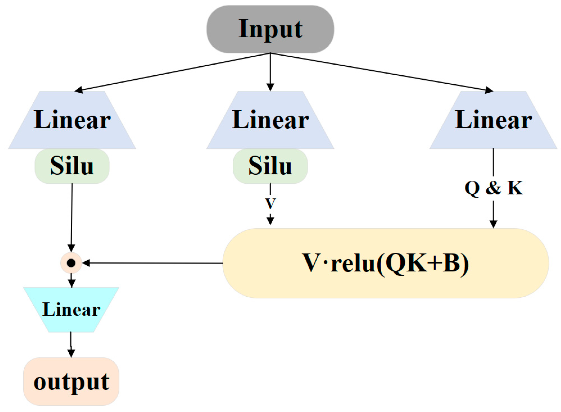
3.3. Gated Attention Mechanism

This paper combines gated technology with the attention mechanism. For feature interaction and enhancement, the attention mechanism can capture the correlations between features. By calculating similarity and weighted scores, the attention mechanism is able to acquire attention to different parts. This process has excellent adaptability to the input data and can accurately capture relevant relationships. To accurately capture the correlations between features, the attention module is focused on the changing trends of the sequence. The gated structure is able to regulate the information flow of attention. This can make the model exclude the influence of noise, and it can result in a more accurate analysis of information with a higher correlation.

The calculation process of the gated attention mechanism is shown in Equation (8).

$$O=\left(U\odot AV\right)W_o$$

(8)

where $O$represents the output. $U and V$ are matrices calculated from the input, and $W$ is the parameter matrix. $A$ is the attention weight matrix, and it is calculated by Equation (9).

$$A=\mathrm{r}\mathrm{e}\mathrm{l}\mathrm{u}\left(\mathcal{Q}\left(Z\right)\mathcal{K}{\left(Z\right)}^{\top }+b\right)$$

(9)

where $\mathrm{r}\mathrm{e}\mathrm{l}\mathrm{u}$ is the activation function, and b is the bias. $Z$ is the same as U and V.

$$Z={\varphi }_z\left(X{W}_z\right), U={\varphi }_u\left(X{W}_u\right),V={\varphi }_v\left(X{W}_v\right)$$

(10)

where $X$ is the input, and $\varphi$ is the activation function, where this paper uses the $Silu$ activation function. Q and K are functions from $Z$. They are similar to a $\mathrm{L}\mathrm{a}\mathrm{y}\mathrm{e}\mathrm{r}\mathrm{N}\mathrm{o}\mathrm{r}\mathrm{m}$ layer structure with one learnable parameter, and they perform scaling and translation operations on each dimension of $Z$. The structure of the gated attention mechanism is shown in Figure 5.

By introducing the gated attention mechanism, the gated structure can be used to regulate the flow of attention information, making the attention computation more efficient. The gated attention mechanism can reduce the possibility of noise and encourage the model to focus on learning relevant information. Additionally, the gated attention mechanism unit utilizes attention information more efficiently through the gated structure, and it requires less resources.

3.4. Gated Attention Mechanism

In this paper, we propose a time series forecasting method based on FLRNN-FGA. First, multivariate time series data are input into the FLRNN module, initializing the RNN model, and integrating all hidden layers through fractional calculus to capture long-term dependencies. Then, the time domain data are transformed into the frequency domain via Fourier transform, selecting low-frequency components to reduce noise interference. Next, a gated attention mechanism is used to capture correlations between features, regulating the transmission of the attention information through the gated structure and finally calculating the model’s output.

As shown in Algorithm 1, the specific steps are as follows: first, the data are input, and the RNN model is instantiated, using fractional calculus to integrate all hidden layers, thus outputting the results of the FLRNN module. Second, the time domain data are transformed into the frequency domain via Fourier transform, and low-frequency components are selected to reduce noise. Finally, the correlations between the features are calculated using the attention mechanism, and the final output is computed through the gated attention layer to obtain the prediction results. This method not only addresses the gradient issues in traditional RNN and LSTM models for long-sequence tasks but also significantly improves prediction accuracy and computational efficiency.

Algorithm 1 FLRNN-FGA
Input: Multivariate time series data
Section 3.1: FLRNN module
	Step 1 Data input instantiation of the RNN model, Equation (1)
	Step 2 Integrating all hidden layers using fractional calculus, Equations (2)~(6)
	Step 3 Output of the FLRNN module
Section 3.2: Frequency Module
	Step 4 Fourier transform converts the time domain into the frequency domain, Equation (7)
	Step 5 Select the low-frequency components to reduce noise.
Section 3.3: Gated Attention mechanism
	Step 6 Capture the correlations between features using the attention mechanism.
	Step 7 Calculate the final output through the gated attention layer using Equation (8).
Output: The output of the prediction results

4. Experiments

To evaluate the performance of FLRNN-FGA, we conduct some experiments on five real-world time series benchmarks and compare them with the corresponding state-of-the-art methods.

4.1. Datasets

The datasets cover multiple major application areas, including energy, economy, transportation, and weather. This provides a more comprehensive test for the performance validation of the model. The real-world multidomain datasets make the model’s prediction results more credible.

Brief descriptions of the datasets:

(a)

Electricity dataset: the hourly electricity consumption records of 321 users from 2012 to 2014;

(b)

ETT dataset: Transformer data from July 2016 to July 2018;

(c)

Weather dataset: 21 meteorological indicator records from every 10 min throughout 2020;

(d)

Exchange dataset: the daily exchange rate records of eight countries from 1990 to 2016;

(e)

Traffic dataset: the hourly road occupancy rates records measured by different sensors on highways in the San Francisco Bay Area.

A sliding window method is adopted to extract data. To avoid the impact of missing data, the time series segments with missing data are excluded from the datasets.

Each dataset used in the experiments is divided into three parts: training set, test set, and validation set. For the ETT dataset, the partitioning ratio of the training set, test set, and validation set is 6:2:2, while for other datasets, the partitioning ratio is 7:1:2.

4.2. Baselines and Evaluation Metrics

To evaluate the effectiveness of the proposed model, this paper selects some current deep learning models in the field of time series forecasting as baselines, including:

⮚

CN: Temporal Convolutional Network, a deep learning method that utilizes one-dimensional dilated convolutions and causal convolutions to process sequential data.

⮚

LSTM: Long Short-Term Memory Network, a deep learning method that uses gated structures to retain long-term information to learn long-term dependencies.

⮚

LSTNet: A method that combines Convolutional Neural Networks and Long Short-Term Memory Networks.

⮚

Informer [37]: A Transformer variant that utilizes sparse self-attention.

⮚

Autoformer [43]: A Transformer variant that employs inter-series attention.

⮚

FEDformer [38]: A Transformer variant that uses the frequency domain to analyze time series data.

The selected baseline models are the ones that have shown good performances in the field of time series data prediction in recent years. Experimental comparisons with these baseline models can demonstrate the feasibility and effectiveness of the proposed model in this paper.

In this paper, mean squared error (MSE) and mean absolute error (MAE) are used as evaluation metrics for the model. These two metrics are the most important indicators to demonstrate the predictive accuracy of a model in time series forecasting.

The calculation of MSE is shown in Formula (11).

$$\mathrm{M}\mathrm{S}\mathrm{E}\left(\mathbf{Y},\widehat{\mathbf{Y}}\right)={\displaystyle \frac{1}{N}}{\sum _{i=1}^N\left(y_i-{\widehat{y}}_i\right)}^2$$

(11)

The calculation process of MAE is shown in Formula (12).

$$\mathrm{M}\mathrm{A}\mathrm{E}\left(\mathbf{Y},\widehat{\mathbf{Y}}\right)={\displaystyle \frac{1}{N}}\sum _{i=1}^N|y_i-{\widehat{y}}_i|$$

(12)

4.3. Experimental Settings

The choice of parameters can affect the experimental results of deep learning models. A batch of data is one input into the network. The size of this batch is called the batch size. A larger batch size can fully utilize the computational resources and parallelism. At the same time, too many input data can reduce the model’s ability to escape from local optimal solutions. Here, a batch size is 32, and it can balance the model’s computational efficiency and its ability to escape from local optimal solutions.

Fractional calculus often leads to increased model complexity and difficulty in network training. Here, the coefficients are pre-computed, and this will result in a relatively small computational burden. Additionally, it is difficult to determine the appropriate fractional order. The optimal order may vary depending on the specific dynamics and time dependence of the data. The most relevant fractional-order interval is (0, 2), and experiments are conducted with the orders [0.2, 0.5, 0.8, 1.0, 1.2, 1.5, 1.8] to find a more appropriate order. The experiments use the electricity dataset and weather dataset for evaluation, and the fractional order is set to 1.8.

In this paper, the Lipschitz recurrent unit is utilized to reconstruct the weight matrix of the hidden layer in the recurrent neural network. The size of the hidden layer vector is set to 128. There are two parameters for controlling the dynamic changes in the system. They are chosen as 0.7 and 0.01. This enables the network to learn the dynamics appropriately while maintaining the stability of the system. Fractional-order integration is introduced to calculate the hidden state of the recurrent neural network. And the fractional-order integration order is set to 1.8, which is an appropriate value determined through experimental comparison. This aims to describe the dynamic behavior of the system more accurately, thereby improving the performance of the model.

The optimizer is ADAM, and the initial learning rate is set to 0.01. After some epochs of training, the learning rate will be adjusted to find the global optimal solution faster in the early stages of training, while avoiding excessive adjustments in the later stages, improving the convergence and stability of the model.

To prevent the model from overfitting the training set, this paper introduces an early stopping mechanism in the experiments. The training will be terminated if there is no improvement on the test set for five consecutive epochs. This mechanism helps stop the training in time after the model performance reaches its peak. To reduce the training time, all the experiments are limited to 20 epochs. The low-frequency part ratio is 0.5. The input length is 336. The hidden layer size of the gated attention module is set to 168.

4.4. Main Results

The results of the multivariate time series forecasting are presented in

Table 1. Forecasting results in terms of MSE and MAE. The best results are highlighted in bold, and the second best results are underlined. The 1st Count means the first number. Smaller values indicate better performance.

Models		FLRNN-FGA (Ours)		FEDformer		Autoformer		Informer		LSTNet		LSTM		TCN
Metric		MSE	MAE	MSE	MAE	MSE	MAE	MSE	MAE	MSE	MAE	MSE	MAE	MSE	MAE
Electricity	96	0.130	0.228	0.183	0.297	0.201	0.317	0.274	0.368	0.680	0.645	0.375	0.437	0.985	0.813
	192	0.151	0.251	0.195	0.308	0.222	0.334	0.296	0.386	0.725	0.676	0.442	0.473	0.996	0.821
	336	0.167	0.269	0.212	0.313	0.231	0.338	0.300	0.394	0.828	0.727	0.439	0.473	1.000	0.824
	720	0.192	0.296	0.231	0.343	0.254	0.361	0.373	0.439	0.957	0.811	0.980	0.814	1.438	0.784
Ettm2	96	0.124	0.240	0.203	0.287	0.255	0.339	0.365	0.453	3.142	1.365	2.041	1.073	3.041	1.330
	192	0.154	0.271	0.269	0.328	0.281	0.340	0.533	0.563	3.154	1.369	2.249	1.112	3.072	1.339
	336	0.194	0.302	0.325	0.366	0.339	0.372	1.363	0.887	3.160	1.369	2.568	1.238	3.105	1.348
	720	0.236	0.344	0.421	0.415	0.422	0.419	3.379	1.338	3.171	1.368	2.720	1.287	3.135	1.354
Exchange	96	0.118	0.255	0.139	0.276	0.197	0.323	0.847	0.752	1.551	1.058	1.453	1.049	3.004	1.432
	192	0.207	0.341	0.256	0.369	0.300	0.369	1.204	0.895	1.477	1.028	1.846	1.179	3.048	1.444
	336	0.353	0.464	0.426	0.464	0.509	0.524	1.672	1.036	1.507	1.031	2.136	1.231	3.113	1.459
	720	1.284	0.823	1.090	0.800	1.447	0.941	2.478	1.310	2.285	1.243	2.984	1.427	3.150	1.458
Traffic	96	0.410	0.265	0.562	0.349	0.613	0.388	0.719	0.391	1.107	0.685	0.843	0.453	1.438	0.784
	192	0.433	0.277	0.562	0.346	0.616	0.382	0.696	0.379	1.157	0.706	0.847	0.453	1.463	0.794
	336	0.451	0.288	0.570	0.323	0.622	0.337	0.777	0.420	1.216	0.730	0.853	0.455	1.476	0.799
	720	0.502	0.306	0.596	0.368	0.660	0.408	0.864	0.472	1.481	0.805	1.500	0.805	1.499	0.804
Weather	96	0.151	0.213	0.217	0.286	0.266	0.336	0.300	0.384	0.594	0.587	0.369	0.406	0.615	0.589
	192	0.206	0.268	0.276	0.336	0.307	0.367	0.598	0.544	0.560	0.565	0.416	0.435	0.629	0.600
	336	0.268	0.320	0.339	0.380	0.359	0.395	0.578	0.523	0.597	0.587	0.455	0.454	0.639	0.608
	720	0.402	0.407	0.403	0.428	0.419	0.428	1.059	0.741	0.618	0.599	0.535	0.520	0.639	0.610
1st Count		37		3		0		0		0		0		0
Improvement		-		18.15%		31.52%		149.36%		281.52%		232.80%		357.32%

.

In this experiment, we compare the performance of FLRNN-FGA (our model) with six other models (FEDformer, Autoformer, Informer, LSTNet, LSTM, and TCN) on five datasets for time series forecasting. The evaluation metrics are mean squared error (MSE) and mean absolute error (MAE). The results show that FLRNN-FGA performs outstandingly on all datasets and prediction windows, achieving the best results in 37 experimental settings, while the second-best model, FEDformer, achieves the best results in only 3 settings. Specifically, on the electricity, Ettm2, exchange, traffic, and weather datasets, the MSE and MAE of FLRNN-FGA are significantly better than those of the other models. For example, on the electricity dataset with a 96-step prediction, FLRNN-FGA has an MSE of 0.130 and an MAE of 0.228, which are 28.42% and 29.02% lower, respectively, than the second-best FEDformer. On the Ettm2 dataset with a 96-step prediction, FLRNN-FGA has an MSE of 0.124 and an MAE of 0.240, which are 38.92% and 19.33% lower, respectively, than the second-best FEDformer. Overall, compared to the other models, the average improvements in MSE and MAE for FLRNN-FGA are 18.15% and 31.52%, respectively, with improvements on some datasets reaching as high as 149.36% (Informer) and 281.52% (LSTNet). This demonstrates that FLRNN-FGA has significant advantages in time series forecasting tasks, maintaining stable and superior performance across different types of time series data.

4.5. Ablation Study

In our approach, there are three major components: the FLRNN, frequency module, and gated attention mechanism. We analyze the effects of each component, and a series of ablation experiments are conducted.

• w/o fractional calculus. 

Firstly, we remove the fractional-order integral; this is the LRNN-FGA model. Then, we eliminate the Lipschitz weight matrix; this is the RNN-FGA model. The changes in performance are shown in

Table 2. Ablation study on fractional-order component.

Models		FLRNN-FGA		LRNN-FGA		RNN-FGA
Metric		MSE	MAE	MSE	MAE	MSE	MAE
Electricity	96	0.130	0.228	0.183	0.273	0.179	0.277
	192	0.151	0.251	0.188	0.281	0.190	0.288
	336	0.167	0.269	0.202	0.295	0.205	0.302
	720	0.192	0.296	0.241	0.328	0.242	0.336
Traffic	96	0.410	0.265	0.588	0.343	0.633	0.364
	192	0.433	0.277	0.585	0.339	0.629	0.366
	336	0.451	0.288	0.609	0.340	0.635	0.365
	720	0.502	0.306	0.636	0.357	0.676	0.377

.

As can be seen in Table 2, fractional-order integration can effectively enhance the prediction performance of the model. The fractional-order description of complex systems provides more useful information for the model, and it makes the final prediction results more accurate. In this paper, the Lipschitz weight matrix is introduced to address the gradient issue. The performance difference between LRNN-FGA and RNN-FGA is relatively small.

• w/o frequency module and gated structure, respectively. 

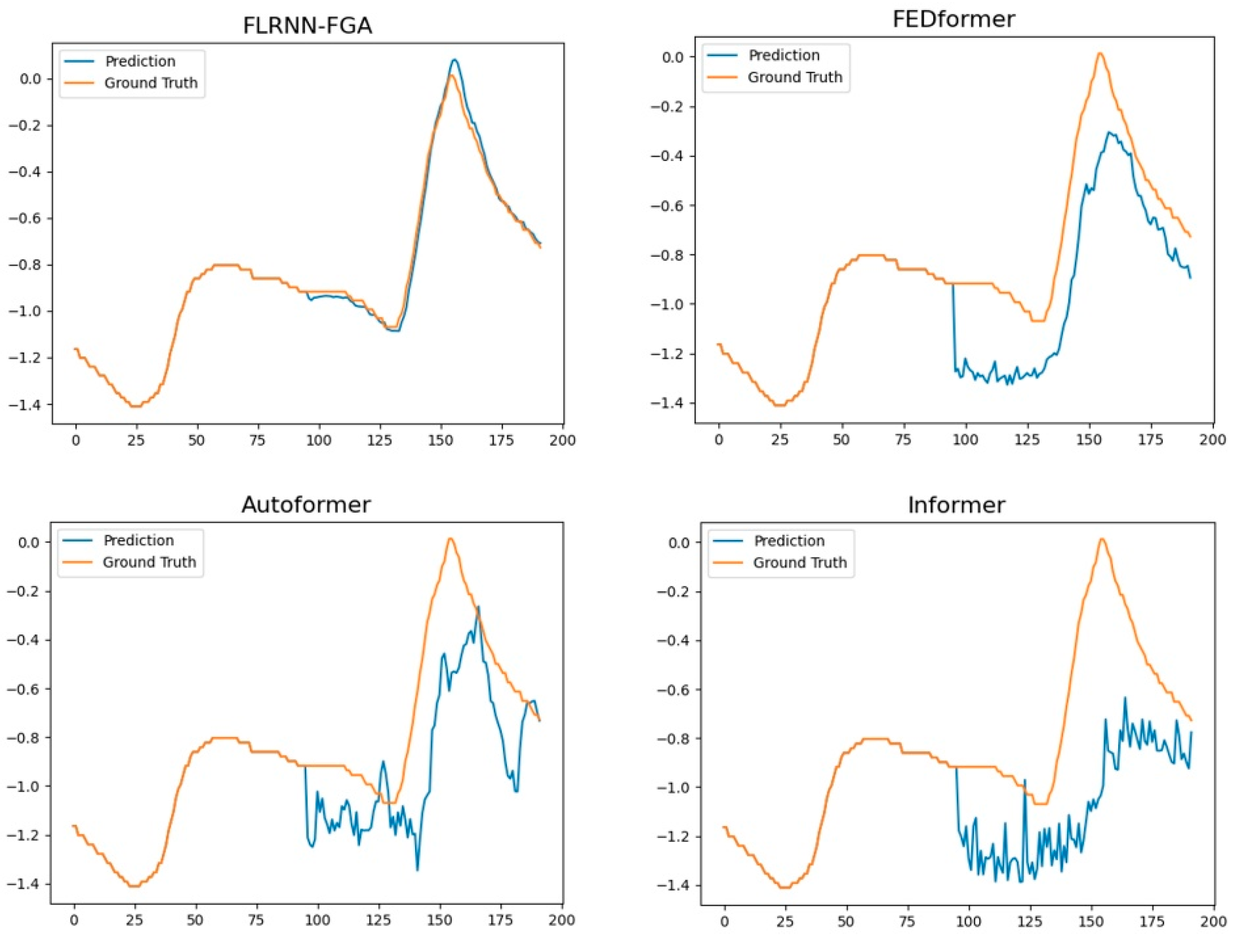
When the frequency module is removed, it is the FLRNN-GA model. When the gated structure is removed, it is the FLRNN-FA model. The frequency processing can reduce the number of parameters to improve prediction accuracy. The gated structure can help the attention mechanism process the similarity information of the data. The experimental results are shown in

Table 3. Ablation study on frequency module and gated structure.

Models		FLRNN-FGA (Ours)			w/o Gated Structure			w/o Frequency Module
Metric		MSE	MAE	Paras/k	MSE	MAE	Paras/k	MSE	MAE	Paras/k
ETTh2	96	0.188	0.305	355.76	0.335	0.395	381.46	0.312	0.374	752.24
	192	0.236	0.340	380.52	0.434	0.457	406.23	0.406	0.432	777.01
	336	0.266	0.363	417.68	0.428	0.447	443.38	0.684	0.580	814.16
	720	0.337	0.421	516.75	2.019	0.976	542.46	1.225	0.751	913.23
Ettm2	96	0.124	0.250	355.76	0.190	0.278	381.46	0.201	0.284	752.24
	192	0.154	0.271	380.52	0.256	0.332	406.23	0.260	0.328	777.01
	336	0.194	0.302	417.68	0.335	0.382	443.38	0.318	0.368	814.16
	720	0.236	0.344	516.75	0.443	0.441	542.46	0.489	0.471	913.23

, which displays the MAE, MSE, and number of parameters (Paras).

It can be seen that the FLRNN-FGA model has a lower number of parameters and lower MSE and MAE compared to the others. This indicates that the frequency module and the gated attention mechanism can decrease the parameters and improve the model’s accuracy. The FLRNN-FGA model can obtain the better results.

4.6. Visualization

To facilitate a clear comparison between the different models, we visualize the prediction results on the ETTm2 dataset with a 96-step output horizon. We compared three recent baseline models: FEDformer, Autoformer, and Informer. The visualization of the prediction results is shown in Figure 6. In contrast, among the various models, the prediction results of FLRNN-FGA are closer to the ground truth results and exhibit superior performance.

4.7. Computational Efficiency Analysis

In this section, we perform a comparative analysis of the computational efficiency of the models on the ETTm2 dataset. As shown in

Table 4. Computational efficiency analysis on the ETTm2 dataset (predict-96). The symbols “M”, “G”, and “S” are used to denote the units for “#Para”, “Memory” and “Time”, respectively, representing million bytes, gigabytes, and seconds, respectively. Smaller values indicate better performance.

	#Para (M)	Memory (G)	Time (S)	MSE
Informer	62.80	1.54	52	0.365
FEDformer	83.70	2.44	174	0.203
Autoformer	59.70	1.97	38	0.255
FLRNN-FGA	1.60	0.49	45	0.124

, we select models with good MSE for the comparison analysis, including FEDformer, Informer, and Autoformer. As we can observe, our proposed FLRNN-FGA model has the smallest number of parameters and the lowest memory usage, which are 1.60 M and 0.49 G, respectively. Moreover, the FLRNN-FGA model also has a shorter training time. Overall, our proposed efficiency analysis indicates that FLRNN-FGA achieves a good balance between computational resources and prediction accuracy.

5. Conclusions

Recurrent neural network (RNN) models establish temporal dependencies for time series data. Many studies have demonstrated the effectiveness of RNN models on time series data. However, gradient explosion and gradient vanishing are important issues when applying RNNs to time series tasks. And the prediction accuracy is not high.

To overcome these problems, the FLRNN-FGA is proposed in this paper. This method mainly involves the FLRNN, frequency module, and gated attention mechanism. In the FLRNN module, piecewise recurrent units are introduced to accelerate the processing speed of recurrent units for long sequences without compromising their performance. Fractional-order Lipschitz recurrent units can alleviate gradient issues and accurately capture system dynamics and dependencies, and they improve the prediction accuracy. In the frequency module, the temporal data are transformed into the frequency domain by the Fourier transform. Frequency domain processing can reduce the computational complexity of the model. In addition, the gated attention mechanism combines gated techniques with the attention mechanism. The gated structure can regulate the attention information transmission. This method can handle inter-variable relationships and reduce model parameter count. The extensive experimental results show the effectiveness and excellence of our proposed method, and the ablation experiments further confirm the rationality of the various components of the model. We hope this work can facilitate more future research on the fractional-order method of time series modeling.

References

1. Li, Z.L.; Zhang, G.W.; Yu, J.; Xu, L.Y. Dynamic graph structure learning for multivariate time series forecasting. Pattern Recognit. 2023, 138, 109423. [Google Scholar] [CrossRef]
2. Klein, N.; Smith, M.S.; Nott, D.J. Deep distributional time series models and the probabilistic forecasting of intraday electricity prices. J. Appl. Econom. 2023, 38, 493–511. [Google Scholar] [CrossRef]
3. Khashei, M.; Bijari, M. A novel hybridization of artificial neural networks and ARIMA models for time series forecasting. Appl. Soft Comput. 2011, 11, 2664–2675. [Google Scholar] [CrossRef]
4. Masini, R.P.; Medeiros, M.C.; Mendes, E.F. Machine learning advances for time series forecasting. J. Econ. Surv. 2023, 37, 76–111. [Google Scholar] [CrossRef]
5. Selvin, S.; Vinayakumar, R.; Gopalakrishnan, E.A.; Menon, V.K.; Soman, K.P. Stock price prediction using LSTM, RNN and CNN-sliding window model. In Proceedings of the 2017 International Conference on Advances in Computing, Communications and Informatics (icacci), Udupi, India, 13–16 September 2017. [Google Scholar]
6. Vlahogianni, E.I.; Karlaftis, M.G.; Golias, J.C. Optimized and meta-optimized neural networks for short-term traffic flow prediction: A genetic approach. Transp. Res. Part C Emerg. Technol. 2005, 13, 211–234. [Google Scholar] [CrossRef]
7. Kumar, B.; Yadav, N. A novel hybrid model combining βsarma and lstm for time series forecasting. Appl. Soft Comput. 2023, 134, 110019. [Google Scholar] [CrossRef]
8. Pedregal, D.J.; Young, P.C. Statistical approaches to modelling and forecasting time series. In Companion to Economic Forecasting; Wiley: Hoboken, NJ, USA, 2002; pp. 69–104. [Google Scholar]
9. Li, X.; Li, N.; Ding, S.; Cao, Y.; Li, Y. A novel data-driven seasonal multivariable grey model for seasonal time series forecasting. Inf. Sci. 2023, 642, 119165. [Google Scholar] [CrossRef]
10. Garcia, R.; Contreras, J.; Van Akkeren, M.; Garcia, J. A GARCH forecasting model to predict day-ahead electricity prices. IEEE Trans. Power Syst. 2005, 20, 867–874. [Google Scholar] [CrossRef]
11. Yi, K.; Zhang, Q.; Fan, W.; He, H.; Hu, L.; Wang, P.; An, N.; Cao, L.; Niu, Z. FourierGNN: Rethinking multivariate time series forecasting from a pure graph perspective. Adv. Neural Inf. Process. Syst. 2024, 36. [Google Scholar]
12. Pan, Z.; Jiang, Y.; Garg, S.; Schneider, A.; Nevmyvaka, Y.; Song, D. S2 IP-LLM: Semantic Space Informed Prompt Learning with LLM for Time Series Forecasting. In Proceedings of the Forty-First International Conference on Machine Learning, Vienna, Austria, 21–27 July 2024. [Google Scholar]
13. Liang, J.; Cao, J.; Fan, Y.; Zhang, K.; Ranjan, R.; Li, Y.; Timofte, R.; Van Gool, L. Conv2former: A simple transformer-style convnet for visual recognition. IEEE Trans. Pattern Anal. Mach. Intell. 2024. early access. [Google Scholar]
14. Liang, J.; Cao, J.; Fan, Y.; Zhang, K.; Ranjan, R.; Li, Y.; Timofte, R.; Van Gool, L. Vrt: A video restoration transformer. IEEE Trans. Image Process. 2024, 33, 2171–2182. [Google Scholar] [CrossRef]
15. Polson, N.G.; Sokolov, V.O. Deep learning for short-term traffic flow prediction. Transp. Res. Part C Emerg. Technol. 2017, 79, 1–17. [Google Scholar] [CrossRef]
16. Zeng, A.; Chen, M.; Zhang, L.; Xu, Q. Are transformers effective for time series forecasting? In Proceedings of the AAAI Conference on Artificial Intelligence, Washington, DC, USA, 7–14 February 2023; Volume 37, pp. 11121–11128. [Google Scholar] [CrossRef]
17. Siami-Namini, S.; Tavakoli, N.; Namin, A.S. A comparison of ARIMA and LSTM in forecasting time series. In Proceedings of the 2018 17th IEEE International Conference on Machine Learning and Applications (ICMLA), Orlando, FL, USA, 17–20 December 2018. [Google Scholar]
18. Hinton, G.E. Learning distributed representations of concepts. In Proceedings of the Eighth Annual Conference of the Cognitive Science Society, Amherst, MA, USA, 1–4 August 1986. [Google Scholar]
19. Xiaotong, H.; Chen, C. Time Series Prediction Based on Multi-dimensional Cross-scale LSTM Model. Comput. Eng. Des. 2023, 44, 440–446. [Google Scholar]
20. Bengio, Y.; Simard, P.; Frasconi, P. Learning long-term dependencies with gradient descent is difficult. IEEE Trans. Neural Netw. 1994, 5, 157–166. [Google Scholar] [CrossRef] [PubMed]
21. Pascanu, R.; Mikolov, T.; Bengio, Y. On the difficulty of training recurrent neural networks. In Proceedings of the International Conference on Machine Learning, Atlanta, GA, USA, 16–21 June 2013. [Google Scholar]
22. Hochreiter, S.; Schmidhuber, J. Long short-term memory. Neural Comput. 1997, 9, 1735–1780. [Google Scholar] [CrossRef] [PubMed]
23. Funahashi, K.-I.; Nakamura, Y. Approximation of dynamical systems by continuous time recurrent neural networks. Neural Netw. 1993, 6, 801–806. [Google Scholar] [CrossRef]
24. Li, X.-D.; Ho, J.K.; Chow, T.W. Approximation of dynamical time-variant systems by continuous-time recurrent neural networks. IEEE Trans. Circuits Syst. II Express Briefs 2005, 52, 656–660. [Google Scholar]
25. Trischler, A.P.; D’Eleuterio, G.M. Synthesis of recurrent neural networks for dynamical system simulation. Neural Netw. 2016, 80, 67–78. [Google Scholar] [CrossRef]
26. Lechner, M.; Hasani, R. Learning long-term dependencies in irregularly-sampled time series. arXiv 2020, arXiv:200604418. [Google Scholar]
27. Rubanova, Y.; Chen, R.T.; Duvenaud, D.K. Latent ordinary differential equations for irregularly-sampled time series. Adv. Neural Inf. Process. Syst. 2019, 32. [Google Scholar]
28. Ding, H.; Li, W.; Qiao, J. A self-organizing recurrent fuzzy neural network based on multivariate time series analysis. Neural Comput. Appl. 2021, 33, 5089–5109. [Google Scholar] [CrossRef]
29. Park, H.; Lee, G.; Lee, K. Dual recurrent neural networks using partial linear dependence for multivariate time series. Expert Syst. Appl. 2022, 208, 118205. [Google Scholar] [CrossRef]
30. Erichson, B.; Azencot, O.; Queiruga, A.; Hodgkinson, L.; Mahoney, M. Lipschitz Recurrent Neural Networks. In Proceedings of the International Conference on Learning Representations (ICLR), Vienna, Austria, 4 May 2021. [Google Scholar]
31. Zhao, C.; Dai, L.; Huang, Y. Fractional Order Sequential Minimal Optimization Classification Method. Fractal Fract. 2023, 7, 637. [Google Scholar] [CrossRef]
32. Xia, L.; Ren, Y.; Wang, Y. Forecasting China’s total renewable energy capacity using a novel dynamic fractional order discrete grey model. Expert Syst. Appl. 2024, 239, 122019. [Google Scholar] [CrossRef]
33. Lai, G.; Chang, W.C.; Yang, Y.; Liu, H. Modeling long-and short-term temporal patterns with deep neural networks. In Proceedings of the 41st International ACM SIGIR Conference on Research & Development in Information Retrieval, Ann Arbor, MI, USA, 8–12 July 2018; pp. 95–104. [Google Scholar]
34. Wen, R.; Torkkola, K.; Narayanaswamy, B.; Madeka, D. A multi-horizon quantile recurrent forecaster. arXiv 2017, arXiv:1711.11053. [Google Scholar]
35. Tan, Y.; Xie, L.; Cheng, X. Neural Differential Recurrent Neural Network with Adaptive Time Steps. arXiv 2023. [Google Scholar]
36. Bergsma, S.; Zeyl, T.; Rahimipour Anaraki, J.; Guo, L. C2FAR: Coarse-to-fine autoregressive networks for precise probabilistic forecasting. Adv. Neural Inf. Process. Syst. 2022, 35, 21900–21915. [Google Scholar]
37. Zhou, H.; Zhang, S.; Peng, J.; Zhang, S.; Li, J.; Xiong, H.; Zhang, W. Informer: Beyond efficient transformer for long sequence time-series forecasting. In Proceedings of the AAAI Conference on Artificial Intelligence, Virtual Event, 2–9 February 2021; Volume 35, pp. 11106–11115. [Google Scholar]
38. Zhou, T.; Ma, Z.; Wen, Q.; Wang, X.; Sun, L.; Jin, R. Fedformer: Frequency enhanced decomposed transformer for long-term series forecasting. In Proceedings of the International Conference on Machine Learning, Baltimore, MD, USA, 17–23 July 2022. [Google Scholar]
39. Sun, Y.; Dong, L.; Huang, S.; Ma, S.; Xia, Y.; Xue, J.; Wang, J.; Wei, F. Retentive Network: A Successor to Transformer for Large Language Models. arXiv 2023, arXiv:2307.08621. [Google Scholar]
40. Gu, A.; Dao, T. Mamba: Linear-Time Sequence Modeling with Selective State Spaces. arXiv 2023, arXiv:2312.00752. [Google Scholar]
41. Vaswani, A.; Shazeer, N.; Parmar, N.; Uszkoreit, J.; Jones, L.; Gomez, A.N.; Kaiser, Ł.; Polosukhin, I. Attention is all you need. Adv. Neural Inf. Process. Syst. 2017, 30, 5998–6008. [Google Scholar]
42. Podlubny, I. Fractional Differential Equations; Academic Press: San Diego, CA, USA, 1999. [Google Scholar]
43. Wu, H.; Xu, J.; Wang, J.; Long, M. Autoformer: Decomposition transformers with auto-correlation for long-term series forecasting. Adv. Neural Inf. Process. Syst. 2021, 34, 22419–22430. [Google Scholar]
Figure 1. The framework overview of FLRNN-FGA: the FLRNN is to improve the prediction accuracy and mitigate gradient vanishing and exploding problems; the frequency module reduces the computational complexity by Fourier transform; the GA combines gated techniques with an attention mechanism to reduce model parameter count and improve efficiency.
Fractalfract 08 00433 g001
Figure 2. Fractional-order Lipschitz Recurrent Neural Network.
Fractalfract 08 00433 g002
Figure 3. Piecewise recurrent units.
Fractalfract 08 00433 g003
Figure 4. Frequency module.
Fractalfract 08 00433 g004
Figure 5. The structure of gated attention mechanism.
Fractalfract 08 00433 g005
Figure 6. Visualization of 96-step results on the ETTm2 dataset.
Fractalfract 08 00433 g006