Voltage Controller Design for Offshore Wind Turbines: A Machine Learning-Based Fractional-Order Model Predictive Method

Abstract

Integrating renewable energy sources (RESs), such as offshore wind turbines (OWTs), into the power grid demands advanced control strategies to enhance efficiency and stability. Consequently, a Deep Fractional-order Wind turbine eXpert control system (DeepFWX) model is developed, representing a hybrid proportional/integral (PI) fractional-order (FO) model predictive random forest alternating current (AC) bus voltage controller designed explicitly for OWTs. DeepFWX aims to address the challenges associated with offshore wind energy systems, focusing on achieving the smooth tracking and state estimation of the AC bus voltage. Extensive comparative analyses were performed against other state-of-the-art intelligent models to assess the effectiveness of DeepFWX. Key performance indicators (KPIs) such as MAE, MAPE, RMSE, RMSPE, and R² were considered. Superior performance across all the evaluated metrics was demonstrated by DeepFWX, as it achieved MAE of [15.03, 0.58], MAPE of [0.09, 0.14], RMSE of [70.39, 5.64], RMSPE of [0.34, 0.85], as well as the R² of [0.99, 0.99] for the systems states [X₁, X₂]. The proposed hybrid approach anticipates the capabilities of FO modeling, predictive control, and random forest intelligent algorithms to achieve the precise control of AC bus voltage, thereby enhancing the overall stability and performance of OWTs in the evolving sector of renewable energy integration.

1. Introduction

Incorporating intelligent models has significantly improved control strategies utilized in offshore wind turbines (OWTs) for alternating current (AC) bus voltage regulation in recent years. Demand for intelligent and effective control mechanisms has increased considerably, paralleling the complexity of renewable energy systems. This introductory section explores the importance of intelligent models, focusing on recent developments in the field that emphasize their key role in enhancing the reliability and effectiveness of OWTs. Significant development has occurred in renewable energy control strategies due to recent advances in intelligent mathematical modeling. Integrating intelligent models has been crucial in achieving precision and resilience in offshore wind energy systems characterized by their dynamics. This section looks into the state-of-the-art advancements that have impacted control methodologies related to AC bus voltage in OWTs. In addition, fractional-order (FO) controllers are implemented in power systems that incorporate renewable energy sources (RESs) (wind, solar, photovoltaic, etc.). The work conducted in [1] provides a comprehensive review of the FO techniques to the RES. An approach was proposed in [2] to address the issue of low inertia resulting from incorporating RES into the power grid. This approach implements an optimized intelligent FO integral controller. A fuzzy-tuned FO proportional/derivative (PD) method for hybrid system load frequency and its control incorporating wind, solar photovoltaic, fuel cells, as well as battery storage systems has been proposed in [3]. An FO frequency controller, explicitly designed for implementation in electrical power infrastructures employing RES, was presented in [4]. The utilization of the FO P-resonant controller is investigated in [5]. Its application is to regulate grid connection supply in the context of hybrid RES. This controller aims to reach improved stabilization speed, even in a fluctuating power supply. A parameterized FO proportional/integral/derivative (PID) is discussed in [6] for a hybrid renewable energy system that supplies continuous power through a photovoltaic and wind energy conversion system (WECS). The analysis of an adaptive FO sliding mode-based disturbance observer integrated with a robust controller is detailed in [7] to regulate the frequency of the wind/diesel power system.

An algorithm is introduced in [8] for wind turbine power control. The algorithm utilizes a FO synergetic PID controller based on a particle swarm optimization (PSO) technique. In [9], FO controllers were used to model and regulate wind conversion systems incorporating hybrid generators. Furthermore, using FO control combined with traditional synergetic control theory, as described in [10], eliminates the unintended chattering problem in multi-rotor wind power systems that employ asynchronous generator-based variable speed. In [11], an approach for controlling multi-rotor wind energy systems is presented utilizing FO fuzzy control. A wind turbine system utilizing an FO permanent magnet synchronous generator is enhanced with a robust adaptive fractional sliding-mode controller to achieve superior tracking precision, rapid response speed, and robustness, as proposed in [12]. This control methodology combines FO and fuzzy control techniques, providing a more resilient strategy. A recent study conducted in [13] delivers a control strategy combining neural networks (NNs) and FO control to enhance the optimization of reactive/active power in dual-rotor wind turbine systems with changing speeds. In [14], a model called adaptive FO fault-tolerant sliding mode control is introduced. This approach is designed to enable the fault-tolerant management of a wind energy conversion system that utilizes an induction generator. The main objective of this control strategy is to achieve maximum power point tracking. In [15], a FO-PID controller is developed for load frequency regulation in power networks that accommodate wind turbines. A hybrid PSO and gravitational search method FO PID are employed in [16] to optimize the operation of voltage source converters for offshore wind farms (OWFs) connected to high-voltage direct current transmission lines. In [17], the application of fractional calculus theory (FCT) improved the performance and effectiveness of the super-twisting algorithm (STA) for controlling the wind power system with an asynchronous generator. Therefore, the integration of the PSO algorithm is investigated in [18] to implement FO PI controllers. The objective is to guarantee the stability of the wind turbine system even while it is running under faulty conditions.

In [19], an approach called Adaptive Reinforcement Learning Takagi and Sugeno Interval Type II Fuzzy Fractional Sliding Mode Observer is presented. This methodology accurately estimates faults and disturbances in a wind turbine using a doubly fed induction generator (DFIG). Considering a shortage of knowledge about uncertainty bounds in real-world situations, an adaptive observer is developed to solve this challenge. Interval Type II fuzzy rules/sets are encompassed to manage the uncertainty associated with membership functions. The observer’s gains are tuned using Proximal Policy Optimization as an implementation of reinforcement learning. In [20], FO adaptive back-stepping control enhances generator-based wind turbines’ maximum power point tracking performance. This is achieved by adjusting for disturbance and uncertainty terms.

Similarly, an FO sliding mode control method is employed in [21] to enhance the performance of the hybrid drive wind turbine during transient operation. Using a direct-speed FO PI controller, as described in [22], can solve the problem of maintaining low-voltage ride-through capabilities in WECS. This method enhances the efficiency of extracting the maximum power from wind turbines.

Model predictive control (MPC) is a commonly used technique employed in wind turbines and wind farms. In [23], a distributed MPC was developed to analyze the frequency response of direct current (DC)-operated OWFs. The use of feedback linearization MPC is also investigated in [24] for a WECS that is generator-based. The objective of this control strategy is to achieve maximum power point tracking. This design aims to eliminate any non-linearity in the system, minimize the computational load of the MPC, and enhance the system’s performance. Wind power generation systems are subject to variations in wind speed, which can affect their stability. A parameter-adaptive robust control was proposed in [25] to tackle this challenge. This method utilizes Bayesian optimization to enable the controller parameters to self-optimize. In order to manage power, reposition floating OWTs, and preserve structural stability, MPC was introduced in [26]. In [27], a further-improved approach enhances the MPC regulation of wind turbine peak shaving. In [28], an MPC coordinated control technique was presented to enhance wind turbines’ grid reliabilities, incorporating permanent magnet synchronous generators (PMSGs) that concentrate on managing active/reactive power. In [29], the incorporation of wind turbines into the classic load frequency control system is manifested to increase the RES generation level by decreasing the costs associated with electricity generation and addressing the issues caused by fake data injection attacks. The possibility of utilizing finite space MPC to establish an interaction between wind farms and the electric grid is investigated in [30]. The objective is to improve the output from the DFIG while considering the fault ride-through technique. In this regard, the summary of the reviewed methodologies is presented in

Table 1. Summary of the reviewed literature.

Control Methodology	Plants	Advantages	Disadvantages	Ref.
FO-IC	Power systems with RES	Improved precision and resilience in energy systems; handle dynamics effectively.	May be complex to implement and tune.	[2]
FO-PD	Hybrid system load frequency including RES	Enhanced load frequency control; can handle hybrid energy sources effectively.	Complexity in controller design and tuning.	[3]
FO	Electrical power infrastructures with RES	Designed specifically for RES; improves stability and performance.	Requires careful parameter tuning.	[4]
FO-PRC	Grid connection supply in hybrid RES	Improves stabilization speed and performance even with fluctuating power supply.	May not be suitable for all types of power fluctuations.	[5]
FO-PID	RES	Continuous power supply regulation; adaptable to different renewable sources.	Complexity in parameterization and maintenance.	[6]
AFO-SMC	Wind/diesel power systems	Enhanced disturbance rejection and robustness.	May be complex and computationally intensive.	[7]
FO-PID-PSO	Wind turbine power control	Optimizes control performance with particle swarm optimization (PSO); effective for wind turbine systems.	PSO might be computationally demanding.	[8]
FO	Wind conversion systems	Effective in regulating hybrid generator systems.	Integration complexity with hybrid generators.	[9]
FO	Multi-rotor wind power systems	Eliminates chattering problems in asynchronous generator-based variable speed systems.	Complexity in combining FO and traditional control theories.	[10]
FO-Fuzzy	Multi-rotor wind energy systems	Enhances control precision and robustness through fuzzy logic.	May be complex to design and tune fuzzy rules.	[11]
FO-Fractional SMC	Wind turbine systems with PMSG	Superior tracking precision, rapid response speed, and robustness.	Potential complexity in adaptive control design.	[12]
NN-FO	Dual-rotor wind turbine systems with varying speeds	Enhances the optimization of reactive/active power; integrates neural networks for improved control.	May require significant computational resources for neural network training.	[13]
Adaptive FO-SMC	Wind energy conversion system with induction generators	Achieves maximum power point tracking; fault-tolerant management.	Complex fault-tolerant design and integration.	[14]
FO-PID	Power networks with wind turbines	Effective for load frequency regulation; hybrid PSO and gravitational search methods enhance optimization.	Complexity in combining multiple optimization techniques.	[15]
FO-PID-PSO	Voltage source converters for OWTs	Optimizes operation and enhances the performance of converters.	Requires complex algorithm integration and parameter tuning.	[16]
FO-SMC-STA	Wind power system with an asynchronous generator	Improves performance and effectiveness in controlling wind power systems.	Complexity in integrating FO control with STA.	[17]
FO-PI-PSO	Wind turbine systems	Enhances stability even under faulty conditions through PSO integration.	Implementation complexity with fault tolerance.	[18]
Adaptive RL-FO	Wind turbines with DFIG	Accurate fault and disturbance estimation; handle uncertainty with adaptive observers.	Complexity in reinforcement learning and adaptive observer design.	[19]
FO Adaptive Back-Stepping Control	Generator-based wind turbines	Enhances maximum power point tracking performance by adjusting for disturbances.	Potential complexity in back-stepping design.	[20]
FO-SMC	Hybrid drive wind turbines	Improves performance during transient operations.	Implementation complexity and need for precise tuning.	[21]
FO-PI	WECS	Maintains low-voltage ride-through capabilities; enhances the efficiency of power extraction.	Potential complexity in maintaining ride-through capabilities.	[22]
MPC	DC-operated OWFs	Analyze frequency response; improve system performance.	Distributed control might be complex to implement and coordinate.	[23]
Feedback Linearization MPC	Generator-based WECS	Achieves maximum power point tracking by minimizing non-linearity.	May increase the computational load and complexity of the system.	[24]
Parameter-Adaptive	Wind power generation systems	Use Bayesian optimization for the self-optimization of controller parameters; handle wind speed variations.	Complexity in parameter adaptation and robustness.	[25]
MPC	Floating offshore wind turbines	Manag power, reposition floating turbines, and preserve structural stability.	Complexity in floating system control and stability management.	[26]
MPC	Wind turbine peak shaving	Enhances the regulation of peak power generation.	May require advanced MPC techniques and tuning.	[27]
MPC	Wind turbines with PMSG	Enhances grid reliability; manages active/reactive power effectively.	Coordination among multiple turbines and PMSGs can be complex.	[28]
Protector	Power systems with wind turbines	Increases RES generation and addresses issues related to fake data injection attacks.	Integration complexity and potential cybersecurity concerns.	[29]
Finite Space MPC	Interaction between wind farms and electric grid	Improves output from DFIG and considers fault ride-through technique.	Finite space MPC implementation can be complex and computationally demanding.	[30]

.

Although significant progress has been achieved in control techniques, there is still a noticeable gap in reaching the highest tracking smoothness, predictive control, and estimating accuracy level in OWTs. This gap presents a challenge in successfully incorporating RES into the electrical power grid. It is essential to address this problem to guarantee the stability and effectiveness of OWTs. Consequently, this paper presents a Deep Fractional-order Wind turbine eXpert control system (DeepFWX) as a controller, providing a comprehensive method to enhance tracking, predictive control, and state estimation precision. DeepFWX is a hybrid PI-FO model predictive RF AC bus voltage controller intended for OWTs. By integrating the advantages of FO modeling, predictive control, and random forest algorithms, DeepFWX is developed. Consequently, the contributions of the work are highlighted as follows:

• A hybrid PI-FOMPC random forest AC bus voltage controller for OWT.
• Focus on addressing OWT challenges, ensuring smooth voltage tracking and state estimation.
• Comparative analyses regarding other intelligent models.
• Superior performance demonstrated across key metrics: mean absolute error (MAE), mean absolute percentage error (MAPE), root mean squared error (RMSE), root mean squared percentage error (RMSPE), and R².
• The integration of FO modeling, predictive control, and random forest algorithms for precise voltage control.

Overall, the non-linear turbine dynamics, the variability in wind conditions, and the complexities of integrating renewable energy sources into the power infrastructure are among the numerous challenges of smooth voltage tracking and state estimation in OWTs. Particularly, the fluctuating and unpredictable character of wind impedes the accurate tracking of voltage, affecting the power output and, as a result, the voltage. Furthermore, the precise estimation and control of the turbine’s state are further complicated by the high level of non-linearity in its dynamic response. Through its hybrid control system, which integrates advanced algorithms with FO modeling, DeepFWX handles these challenges. The FO model improves the smoothness of voltage tracking by more accurately depicting the system’s dynamic behavior than traditional integer-order models, thereby providing enhanced flexibility and precision. The model predictive control component anticipates future system behaviors and adjusts control actions accordingly, thereby ensuring stable voltage regulation and mitigating the impact of wind variability. Additionally, the integration of RF algorithms improves state estimation by efficiently managing intricate, non-linear relationships and minimizing prediction errors, a critical component of ensuring stable control in dynamic environments.

This paper is organized as follows: Section 2 includes the relevant principles. The applied control methodologies, and the detailed explanation of the architecture of the DeepFWX controller are manifested by Section 3 and Section 4, respectively. Section 5 and Section 6 provide results, demonstrating the model’s effectiveness. As the final step, Section 7 concludes the study.

2. Relevant Principles

AC bus voltage control in OWTs is an important aspect of the controlling system designed to ensure the stability and reliable operation of the power grid. The AC bus voltage refers to the voltage level in the AC electrical bus that connects various components within the wind turbine system. This voltage must be carefully controlled to meet specific operational requirements and standards.

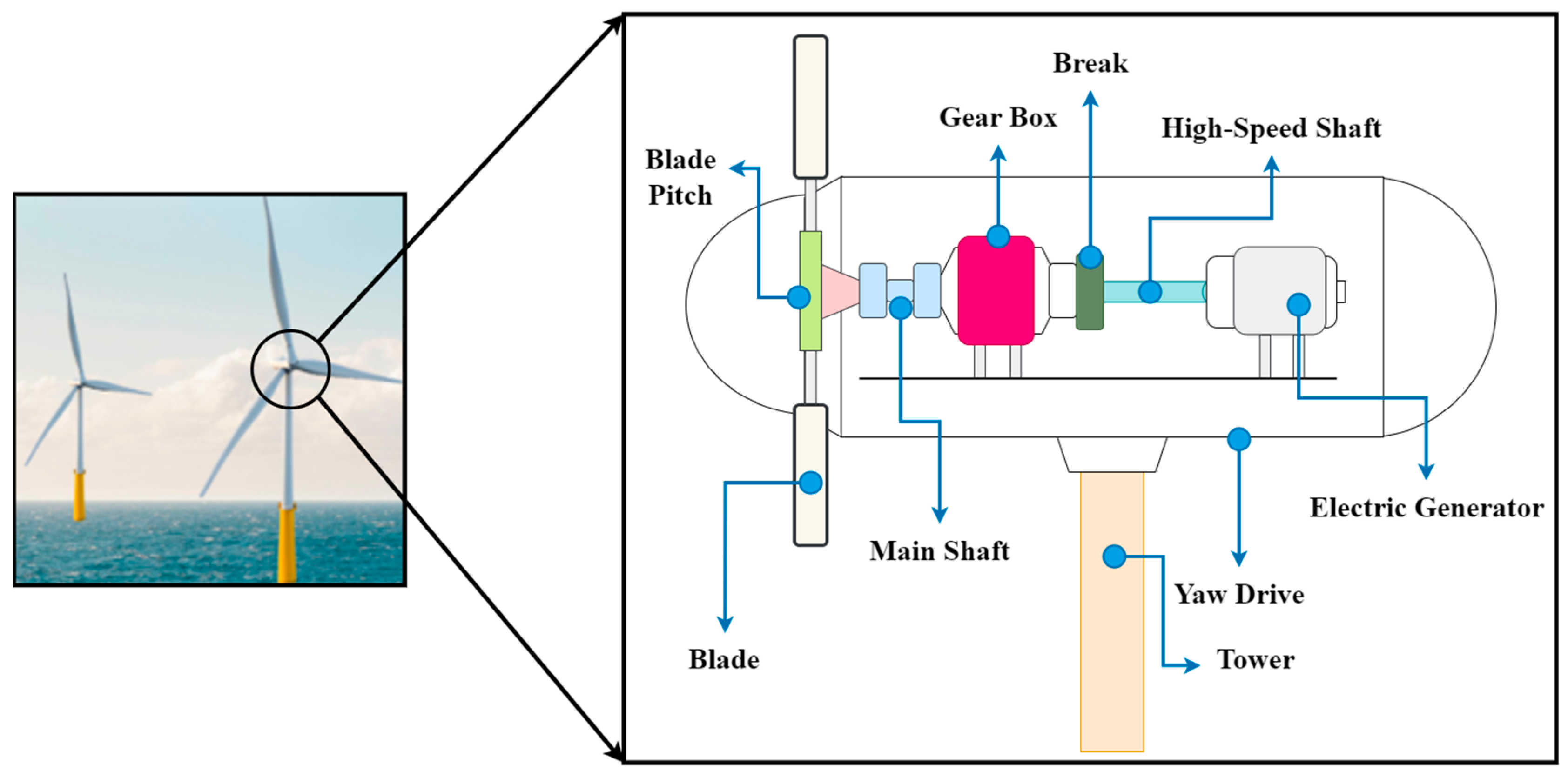
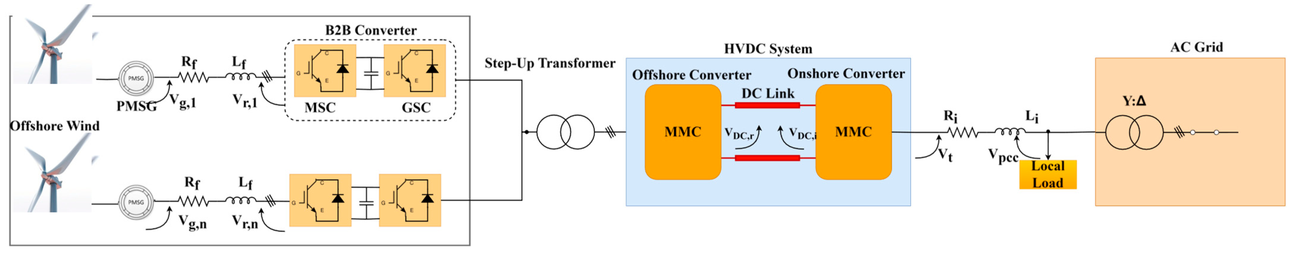
2.1. Offshore Wind Turbines

OWTs represent an important and rapidly expanding renewable energy infrastructure, harnessing the power of wind to generate electricity in maritime environments. These towering structures, anchored in the seabed, utilize the stronger and more consistent winds found offshore, offering a more efficient and reliable energy source than onshore alternatives. The design and engineering of OWTs have evolved to withstand the challenging conditions of open waters, including harsh weather, saltwater corrosion, and the dynamic forces of the sea. Their colossal size and cutting-edge technology enable these turbines to capture substantial amounts of wind energy, converting it into a clean and sustainable power source. With advancements in offshore wind farm projects globally, these turbines contribute significantly to diversifying the energy mix and reducing carbon emissions, which are essential in the transition to sustainable energy technologies. An OWT is conceptualized in Figure 1.

From Figure 1, an OWT’s rotating component consists of a hub connected to the main shaft, with three blades positioned within it. The hub houses the mechanism responsible for adjusting the pitch of the blades. Typically constructed from fiberglass occasionally reinforced with Kevlar, these hollow blades are designed to optimize aerodynamics, ensure maximum efficiency, and minimize noise generation during movement. As wind flows across a blade, a pressure difference on either side generates lift and drag. The resultant lift, surpassing drag, propels the rotor into rotation. Most turbines incorporate three variable-length blades, with the largest wind turbine featuring blades exceeding 100 m. The hydraulic system governs the blade pitch, modifying the angle of the blades in response to wind conditions. This adjustment controls rotor speed and, consequently, the energy generated. The low-speed main shaft, a drivetrain component, is linked to the rotor and rotates at a speed of 8–20 revolutions per minute (RPM). The gear system within the gearbox ensures a consistent output shaft frequency, facilitating the use of a synchronous generator. The generated electricity is then directed to a transformer station and into the grid.

The main bearing supports the rotating low-speed shaft, minimizing friction to protect against damage caused by rotor forces. The turbine structure, mounted on a reinforced concrete foundation, comprises a tubular steel tower typically assembled on-site in three sections. Taller towers capitalize on increased wind speed at greater heights, enhancing energy capture. The yaw drive is responsible for orienting the turbine in alignment with the wind, and the yaw drive, in conjunction with the wind vane, ensures proper alignment with the wind direction. Aerodynamic braking is employed to halt turbine operation, orienting the blades to minimize wind resistance. The rotor brake serves as a parking brake during maintenance, preventing rotor movement. Wind-driven blade rotation transmits rotational force via a shaft, gearbox, and generator, converting mechanical energy into electricity through copper windings turning within a magnetic field. Wind direction and speed are monitored by a wind vane and anemometer, respectively, with a computer utilizing these data to adjust blade pitch and optimize turbine efficiency.

OWTs come in various designs tailored to specific environmental conditions and project requirements. Fixed-bottom turbines, the most common type, are anchored directly to the seabed using monopile or jacket foundations. Monopile foundations are based on a single, large-diameter steel tube that goes into the seabed, stabilizing the wind turbine tower. On the other hand, jacket foundations utilize a lattice-like structure anchored to the seabed, distributing the load more evenly. Floating OWTs are another category gaining prominence in deeper waters where fixed-bottom solutions are impractical. These turbines are tethered to the seabed using mooring systems, allowing them to operate in deeper ocean areas. Floating platforms can be categorized into various designs, such as tension-leg, spar buoy, semi-submersible, and barge configurations. Their adaptability to deeper waters expands the potential offshore wind farm locations, tapping into untapped wind resources.

Innovations include vertical-axis wind turbine technologies (VAWTs), an alternative to horizontal-axis wind turbines (HAWTs). VAWTs can operate regardless of wind direction and potentially reduce maintenance costs. However, HAWTs remain more prevalent in offshore installations due to their established technology and higher efficiency in harnessing wind energy.

2.2. Modular Multilevel Converter (MMC)

The MMC stands out as an advanced power electronics technology with extensive application in OWTs. This converter topology, known for its scalability and ability to handle high voltage levels efficiently, is pivotal in converting the variable and often unpredictable output from OWFs into stable, grid-compatible electricity. In OWTs, the MMC is commonly employed as a part of the power conversion system within the wind turbine’s substation. Its modular structure, consisting of multiple power electronic cells, enables it to achieve high-voltage levels with improved efficiency and reduced energy losses. The MMC’s capability to handle the demanding conditions of offshore environments, including saltwater exposure and challenging weather, makes it an ideal choice for converting the variable AC output generated by the wind turbine into a stable DC voltage for transmission to onshore facilities. The offshore environment poses unique challenges for power transmission due to the distance between the wind turbines and onshore connections, necessitating efficient and reliable power conversion systems. The MMC addresses these challenges by providing a compact and scalable solution that enhances the overall performance of offshore wind energy systems.

Moreover, the MMC’s ability to operate with high-voltage direct current (HVDC) transmission systems makes it particularly suitable for connecting OWFs to onshore grids. This is crucial for optimizing power transmission over long distances, minimizing transmission losses, and ensuring a more reliable integration of offshore wind energy into the larger electrical grid.

3. Applied Control Concepts and Strategies

This section details the applied control concepts, scheme, and DeepFWX architecture.

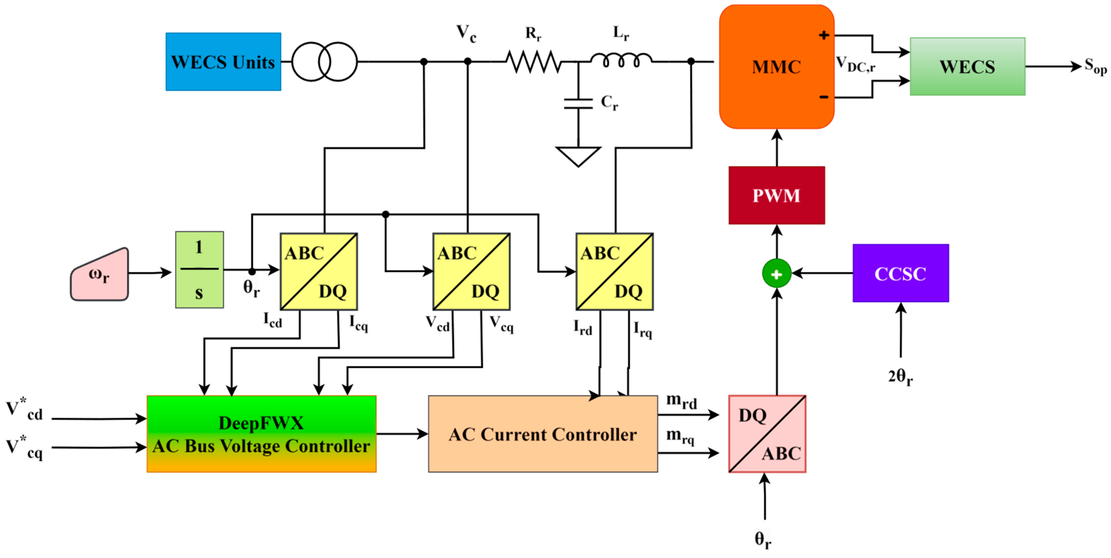
Overall Control Scheme

AC bus voltage control in OWTs ensures stable and reliable power generation. The AC bus, or alternating current bus, serves as the main electrical connection point for various components within the wind turbine, including the generator, power electronics, and auxiliary systems. Maintaining a consistent and stable AC bus voltage is crucial for optimizing the performance and longevity of these components. One key element in AC bus voltage control is power electronic devices such as voltage source converters (VSCs) or MMCs. These converters are integral to the wind turbine’s power conversion system and regulate the AC bus voltage. They achieve this by setting the voltage’s magnitude and phase, ensuring it remains within predefined limits. In the context of OWTs, where environmental conditions can be harsh and unpredictable, the AC bus voltage control system must be robust and adaptive. It should account for variations in wind speed, load fluctuations, and potential grid disturbances. Advanced control algorithms, such as MPC or model algorithmic control (MAC), are implemented to enhance the system’s responsiveness and resilience to changing conditions. The overall system bench and its control scheme are illustrated in Figure 2 and Figure 3:

Figure 3 and Figure 4 show that the OWT’s MMC is a grid-forming converter to the wind-induced generating units (WGUs), supplying collector network voltage. To accomplish this goal, an AC voltage control loop has been developed. With f_r equal to 60 Hz, an integrator provided at an angular frequency of ω = (2πf_r) ABC/DQ transformation angle. The WECS control mode block monitors the converter DC voltage. When the DC voltage reaches its rated value of 110%, the WECS units receive the signal, which causes the control mode of the wind generator to change. In this regard, AC bus voltage dynamics are modulated as follows [31]:

$$C_r\left({\dot{v}}_{cd}-{\omega }_r{v}_{cq}\right)=i_{cd}-i_{rd}$$

(1)

$$C_r\left({\dot{v}}_{cq}+{\omega }_r{v}_{cd}\right)=i_{cq}-i_{rq}$$

(2)

where i_cd and i_cq denote the direct and quadrature axes of grid-injected currents, respectively. Accordingly, the correlations of AC bus voltages yield as follows:

$$i^{*}rd=-u_{v2d}+\left(C_r{\omega }_r\right)v_{cq}+i_{cd}$$

(3)

$${i^{*}}_{rq}=-u_{v2q}+\left(C_r{\omega }_r\right)v_{cd}+i_{cq}$$

(4)

In the next phase, the DeepFWX (PI-fractional-order model predictive controller (FOMPC)-random forest (RF)) is applied to the system to regulate V_cd and V_cq. Their * equivalents are signals, considered references, that must be tracked. Using the Laplace transforms of the developed equations in (1)–(4), the AC bus voltage control strategy is depicted in Figure 4.

The control schemes shown in Figure 4 employ the following transfer functions:

$$G_{FOMPC-RF}\left(s\right)\cdot G_{c2}\left(s\right)\cdot U_{v2d}\left(s\right)+\left[1-G_{c2}\left(s\right)\right]\cdot {\omega }_r\cdot C_r\cdot V_{cq}\left(s\right)+\left[1-G_{c2}\left(s\right)\right]\cdot I_{cd}\left(s\right)=s\cdot C_r\cdot V_{cd}\left(s\right)$$

$$G_{FOMPC-RF}\left(s\right)\cdot G_{c2}\left(s\right)\cdot U_{v2q}\left(s\right)+\left[1-G_{c2}\left(s\right)\right]\cdot {\omega }_r\cdot C_r\cdot V_{cd}\left(s\right)+\left[1-G_{c2}\left(s\right)\right]\cdot I_{cq}\left(s\right)=s\cdot C_r\cdot V_{cq}\left(s\right)$$

(5)

where, G_c2(s), likewise, I_cq(s) and I_cd(s), as well as U_v2d(s) and U_v2q(s) mitigate the grid current influence on the control variables, respectively. Consequently, based on the resulting equations, the close loop online control transfer function of the system can be formed as follows:

$$G_{v2dq}\left(s\right)={\displaystyle \frac{V_{cdq}\left(s\right)}{{V^{*}}_{cdq}\left(s\right)}}={\displaystyle \frac{s\left(\frac{K_{pv2}}{C_r}\right)+\left(\frac{K_{iv2}}{C_r}\right)}{s^2+s\left(\frac{K_{pv2}}{C_r}\right)+\left(\frac{K_{iv2}}{C_r}\right)}}$$

(6)

$$T{F}_{sys}=G_{FOMPC-RF}\left(s\right)\cdot G_{v2dq}\left(s\right)=G_{FOMPC-RF}\left(s\right)\cdot {\displaystyle \frac{s\left(\frac{K_{pv2}}{C_r}\right)+\left(\frac{K_{iv2}}{C_r}\right)}{s^2+s\left(\frac{K_{pv2}}{C_r}\right)+\left(\frac{K_{iv2}}{C_r}\right)}}$$

(7)

In which ${K_p}_{v2}=2{\zeta }_{v2}{\omega }_{v2}{C}_r$ and ${K_i}_{v2}={{\omega }^2}_{v2}{C}_r$ are the PI-controller parameters. In this regard, ${\zeta }_{v2}$, and ${\omega }_{v2}$ are the damping factor of the online system and natural undamped frequency, respectively. The closed-loop transfer function of Equation (7) is a second-order transfer function, so it has two states, namely X₁ and X₂. In other words, these states are related to AC bus voltage control in OWTs. The X₁ and X₂ states are essential factors in understanding and analyzing the behavior of AC bus voltage control of OWTs.

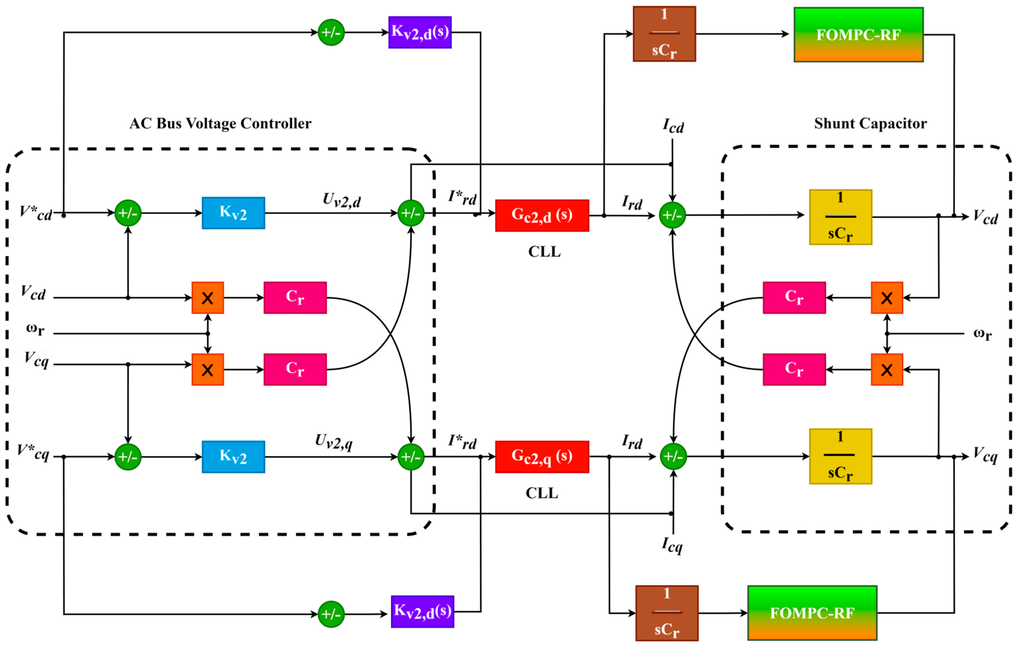
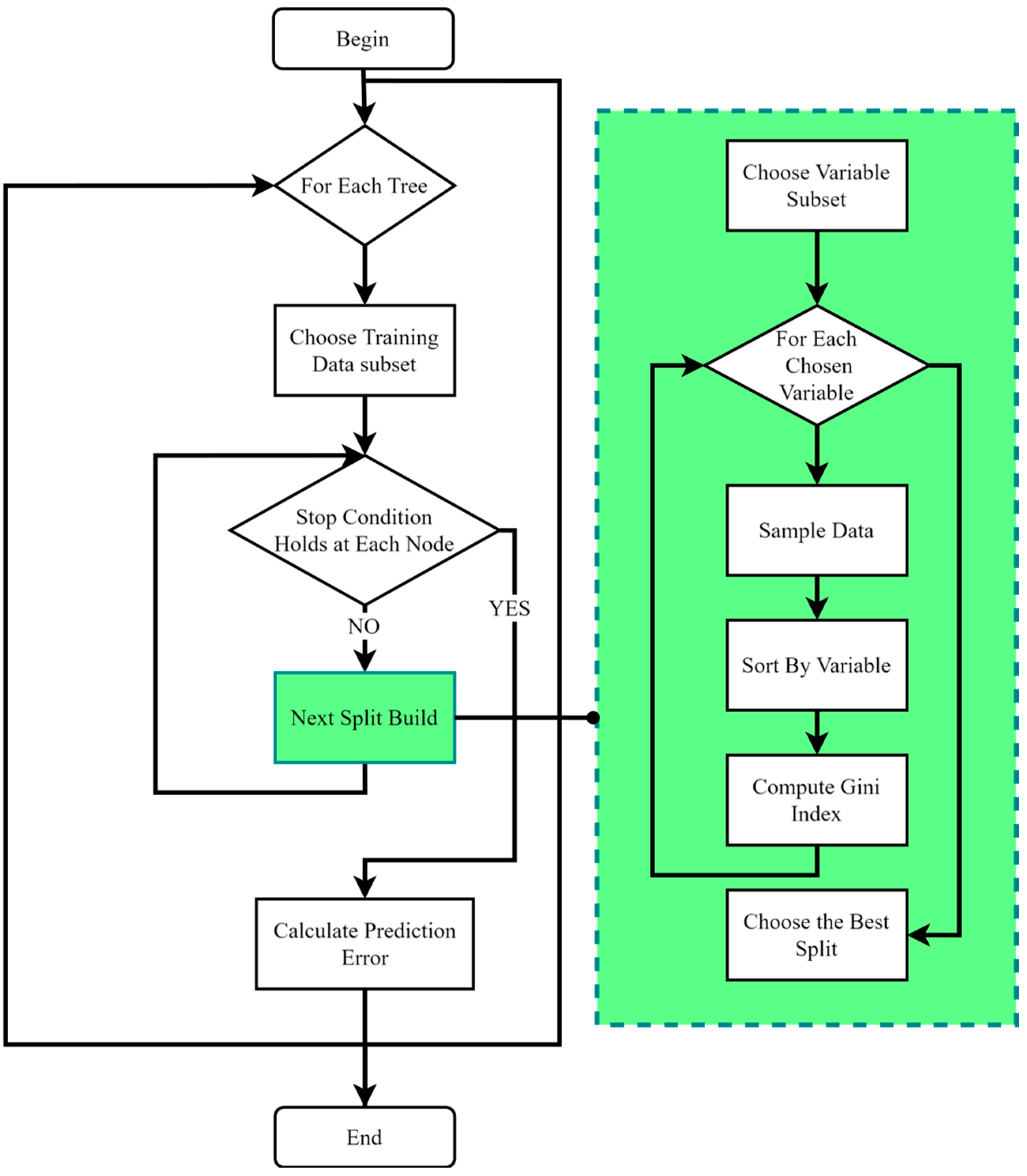
4. DeepFWX: FO Model Predictive Random Forest Controller

MPC is an advanced control technique that utilizes an internal process model to forecast system behavior over a finite time horizon, determines an optimal control signal by minimizing a cost function over that horizon while fulfilling input and state constraints, and only implements the current time step of the optimized manipulated variable profile before repeating the optimization at the next time step. Traditionally, MPC uses integer-order process models within its formulation and optimization. However, many real-world systems exhibit FO dynamics that integer-order differential equations cannot entirely describe. To address this, FOMPC employs FO process models within the MPC technique. This allows it to better model systems with inherent FO behavior, such as diffusive and dispersive processes represented by fractional differential equations rather than ordinary differential equations. FOMPC approximates the fractional derivatives and integrals involved using various numerical techniques and directly incorporates the FO dynamics into the predictive process model and its online optimization. The result is improved control performance for FO plants compared to the conventional integer-order MPC, with benefits such as enhanced reference tracking, disturbance rejection, and stability. However, the extra computational complexity introduced by approximating and working with fractional dynamics also means FOMPC faces greater processing demands than the standard MPC. Consequently, the overall steps of DeepFWX implementation are as follows:

• The implementation of a model predictive controller;
• Tuning the MPC with fractional-order concepts;
• Applying FOMPC on the system for controlling purposes;
• Estimating FOMPC-applied system’s states using the machine learning algorithm of random forest.

In this regard, the FOMPC of DeeFWX is mathematically formulated as follows:

$$J{=}^{\alpha }{\mathcal{I}}_{T_s}^{P{T}_s}q⌊\left(y\left(t\right)-y_r\left(t\right){)}^T\left(y\left(t\right)-y_r\left(t\right)\right)\right]{+}^{\beta }{\mathcal{I}}_{T_s}^{M{T}_s}r⌊\Delta u\left(t{)}^T\Delta u\left(t\right)\right]$$

(8)

where $T_s=0.01$ is the sampling time, and $\mathcal{I}$ is the FO integral. $\alpha$ and $\beta$ denote the FO integral order. The symbols $q$ and $r$ are weighting factors and $y_r$ denotes the desired output. P and M are predictive and control horizons, respectively. The symbol u is the control signal applied to the AC bus voltage in OWT. To discretize $J$, one can use the following [32]:

$$J_{FO}\cong {(\mathrm{Y}-{\mathrm{Y}}_r)}^T\mathrm{Q}\mathsf{\Gamma }\left(T_s,{\alpha }_1\right)\left(\mathrm{Y}-{\mathrm{Y}}_r\right)+{\Delta \mathrm{U}}^T\mathrm{R}\mathsf{\Gamma }\left(T_s,{\alpha }_2\right)\Delta \mathrm{U}$$

(9)

In which Y, $\Delta \mathrm{U}$, and Y_r are defined as follows:

$$\mathrm{Y}=\left[\begin{array}{l}y\left(k+1\right)\hfill \\ y\left(k+2\right)\hfill \\ ⋮\hfill \\ y\left(k+P\right)\hfill \end{array}\right], \Delta \mathrm{U}=\left[\begin{array}{l}\Delta u\left(k\right)\hfill \\ \Delta u\left(k+1\right)\hfill \\ ⋮\hfill \\ \Delta u\left(k+\left(M-1\right)\right)\hfill \end{array}\right], {\mathrm{Y}}_r=\left[\begin{array}{l}{y}_r\hfill \\ y_r\hfill \\ ⋮\hfill \\ y_r\hfill \end{array}\right]$$

(10)

As well, $\mathrm{Q}$ and $\mathrm{R}$ are weighting matrices with the following:

$$\Gamma \left(T_s,{\alpha }_1\right)=T_s^{{\alpha }_1}diag\left(W_N,W_{N-1},\dots ,W_1,W_0\right)$$

(11)

$$\Gamma \left(T_s,{\alpha }_2\right)=T_s^{{\alpha }_2}diag\left(W_M,W_{M-1},\dots ,W_1,W_0\right)$$

(12)

where $W_i={\omega }_i^{-{\alpha }_j}-{\omega }_{\left(i-Z\right)}^{-{\alpha }_j}$ and $Z=P$ for $j=1$, $Z=M$ for $j=2$ and ${\omega }_i^{-{\alpha }_j}$ can be obtained as follows:

$${\omega }_i^{-{\alpha }_j}=\left\{\begin{array}{ll}\left(1-{\displaystyle \frac{1-{\alpha }_j}{i}}\right){\omega }_i^{-{\alpha }_{j-1}}\hfill & i>0\hfill \\ 1\hfill & i=0\hfill \\ 0\hfill & i<0\hfill \end{array}\right.$$

(13)

FO modeling has a precise and adjustable representation of dynamic systems by stretching the concept of differentiation and integration to non-integer (fractional) orders. In contrast to the conventional integer-order models, which employ fixed-order derivatives, FO models enable a continuum of derivative orders, thereby providing improved system behavior approximation and enhanced tuning capabilities. This mathematical foundation is founded on fractional calculus, which is capable of describing the memory and hereditary properties of a variety of materials and processes. FO controllers can enhance the stability, robustness, and efficacy of OWTs by achieving more precise control over system dynamics through the capture of these properties. FO is entirely introduced in [33]. Also, one of its applications in power systems, integrated with AI-driven models, is presented in [34].

For the next phase, RF is implemented to estimate states. RF is an ML algorithm that utilizes an ensemble of decision trees for classification and regression tasks, as illustrated in Figure 5.

Based on Figure 5, RF operates by creating decision trees throughout the training process and determining the class of trees considered most frequently among the trees or the average forecast of the individual trees. Random forest can be employed to estimate the status of OWTs by training a model to comprehend the intricate non-linear connections between the measurements from turbine sensors and the different operational states of the turbine. It can estimate turbine quantities that are difficult to measure directly, such as tower vibrations, shaft torques, and power outputs, based on easier-to-acquire data, such as wind speed, rotor speed, etc. This helps optimize maintenance and operation. Consequently, the proposed capability is important for state estimation, as the accurate prediction of system states is crucial for the preservation of performance and stability by capitalizing on the random forest’s capacity to generate predictions with high accuracy and robustness in the context of high-dimensional data.

For AC bus voltage control in OWFs, the RF can accurately learn the effect of controllable variables such as capacitor bank switching, reactive power adjustments, and turbine terminal voltage changes on the overall bus voltage. It can then perform online short-term predictions of the bus voltage and automatically determine optimum control actions needed to maintain the voltage level within specified bounds under changing electrical loads and turbine power outputs influenced by fluctuating wind conditions. The non-linear control capabilities of random forest improve voltage stability compared to traditional linear control schemes. Consequently, RF is modulated as [35], available in Appendix A. Furthermore, to evaluate the performance of DeepEMS and make a comparison with other models, the KPIs are considered [36,37,38,39], described in Appendix B. The reason for selecting the mentioned KPIs is that insights into the average error amplitude, both in absolute and relative terms, are essential for evaluating the controller’s overall performance and consistency, as provided by MAE and MAPE. RMSPE provides a normalized perspective for comparing performance across various scales, whereas RMSE accentuates larger errors, which reflect the model’s ability to manage significant deviations. The model’s overall predictive potential was validated by R², which quantifies the proportion of variance accounted for by the model. The PI-MPC was implemented in MATLAB by utilizing its control system design tools and robust numerical solvers. The PI-MPC controller, boundary conditions, and necessary system simplifications were facilitated by MATLAB. The RF component was developed and trained on Google Colab using Python (https://www.python.org/).

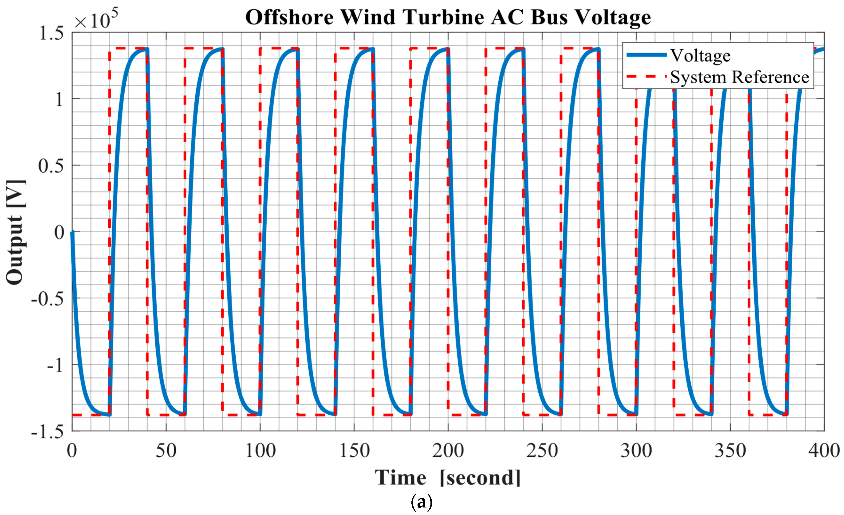
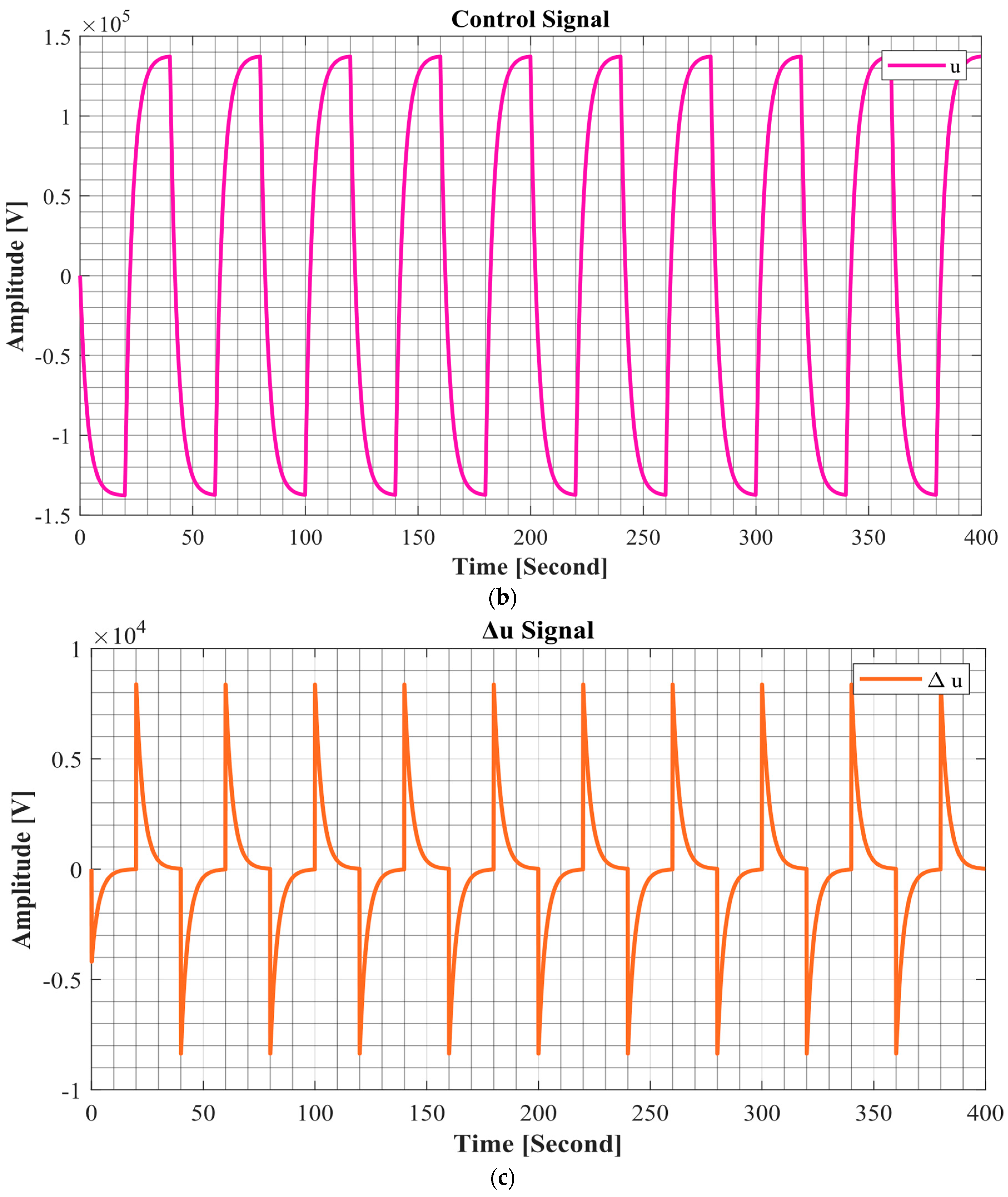
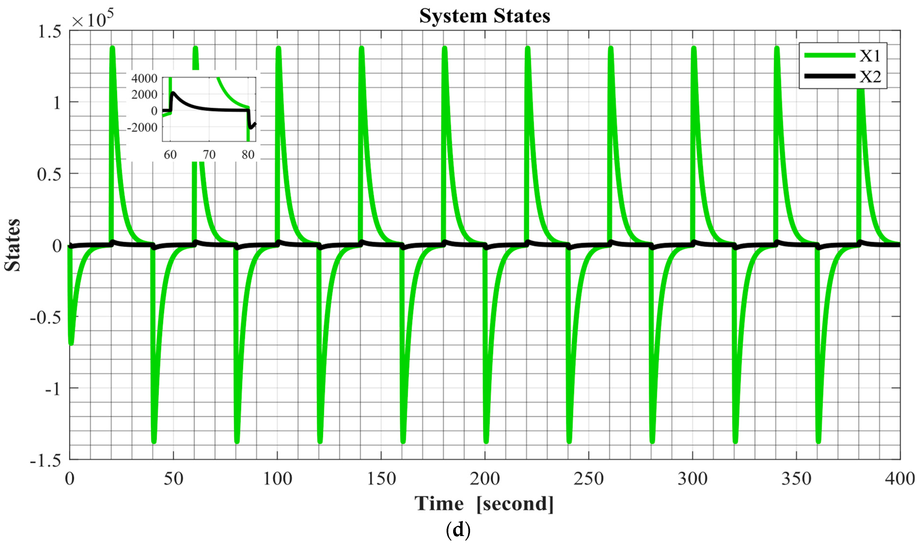
5. Simulations and Results

In this section, the results are presented to assess the performance of the AC bus voltage regulation in an OWT by applying the FOMPC. The simulations were conducted in two phases, with the initial phase dedicated to implementing the FOMPC for AC bus voltage control. The outcomes, encompassing output responses, characteristics of control signals, and the system states, are comprehensively depicted in Figure 6.

A visual representation of the AC bus voltage dynamics, controlled by the FOMPC, is presented in Figure 6a, emphasizing the controller’s impact on the overall system behavior. The characteristics of the control signals generated by the FOMPC are similarly illustrated in Figure 6b, manifesting their role in forming the system’s performance. Additionally, Figure 6c,d portrays the states of the system, offering insights into the internal dynamics of the OWT system influenced by the FOMPC. The effectiveness of the FOMPC is evident in the controlled output responses, well-defined control signals, and stabilized system states. The controlled output responses, well-defined control signals, and stabilized system states affirm the effectiveness of the FOMPC in maintaining the desired performance by the system output ranging from −1.5 × 10⁵ to 1.5 × 10⁵. The control signal graph also performs in the −10⁴ to 10⁴ range. The results of these simulations provide a comprehensive analysis of the practical implications of the DeepFWX. Further analysis and comparison with alternative controllers will be integral to establishing the superiority and robustness of the FOMPC.

For the second phase, the states estimated by RF are the generated data characteristics, and the results are presented in

Table 2. The details of the generated dataset.

	u [kV]	Δu	X1 [kV]	X2 [kV]
Mean	−1.0631	343.55	−1.0937	662.6547
Variance	12,964.39	5.6252	1300	1990
Total Count	4000

, and Figure 7 and Figure 8, indicating that X₁ and X₂ are the states of the systems originating from the OWT form in the Laplace space.

As shown in Figure 7 and Figure 8, density analysis involves creating visual representations, such as density plots or histograms, to illustrate the distribution of values within a dataset, providing insights into the concentration and spread of data points along the range of a variable. The closed-loop transfer function described in Equation (7) is a second-order transfer function. As a result, it comprises two states, denoted as X1 and X2. In the context of offshore wind turbines, these states specifically pertain to AC bus voltage control. Also, the X1 and X2 states are key factors in the behavior of the AC bus voltage control of offshore wind turbines. This technique aids in understanding the frequency and intensity of the predicted values for a given state variable, as seen in the context of the state estimation for X₁ and X₂. In parallel, scatter analysis utilizes scatter plots to visualize the relationship between two variables, assessing how well-predicted values align with the actual observations. A linear pattern in a scatter plot presents a robust correlation between the predicted and actual values, indicative of a successful model. In analyzing the system’s state estimation conducted through RF, density, and scatter plots were generated to understand the model’s performance. For the state estimation of X₁, the density plot depicted a range from 0 to 1.75 × 10⁵, corresponding to the X₁ values from −150,000 to 150,000. This range effectively encapsulated the distribution of the estimated values and showcased the concentration of the predictions within the specified bounds. Similarly, for X₂ state estimation, the density plot presented results ranging from 0 to 0.0012, with X₂ values varying between −2000 and 2000. This representation effectively illustrated the density of the model’s predictions within the designated range and provided insights into the distribution of the estimated X₂ values.

Additionally, scatter analytics were generated for both X₁ and X₂. Despite the wide-ranging values, both the scatter plots exhibited linearity, indicating a strong alignment between the predicted and actual data points. The linear pattern observed in the scatter plots suggests that the random forest model successfully fitted the predicted data to the actual observations. For the final state, the KPIs of the model were computed using the metrics defined in

Table 3. The KPIs for DeepFWX.

Metric	X1	X2
MAE	15.03	0.5797
MAPE	0.09%	0.001374
RMSE	70.39	5.6371
RMSPE	0.34%	0.008548
R2	0.999998	0.999938

.

The KPIs derived from the DeepFWX model for state estimation exhibit noteworthy accuracy and precision. For the estimation of X₁, the model achieved an MAE of 15.03, indicating a minimal average deviation of the predicted values from the actual observations. The MAPE for X₁ was low at 0.09%, highlighting the model’s capability to maintain high accuracy even in relative terms. The RMSE for X₁ was 70.39, reflecting the mean square error associated with the predicted and real values. The RMSPE for X₁, at 0.34%, further underscores the precision of the model’s predictions. The R² for X₁ was exceptionally high at 0.999998, indicating an almost entire model fit to the actual data.

Similarly, for the estimation of X₂, the KPIs demonstrate outstanding performance. The MAE for X₂ was 0.5797, signifying a minimal average absolute deviation of the predicted values from the true observations. The MAPE for X2 was remarkably low at 0.001374%, showcasing the model’s accuracy in percentage terms. The RMSE for X₂ was 5.6371, measuring the error average rates derived in the predicted values. The RMSPE for X₂, at 0.008548%, indicates the precision of the model in relative terms. The R² value for X₂ was exceptionally high at 0.999938, affirming the model’s ability to approximate the observed data closely.

A comprehensive comparison of the DeepFWX model with several alternative models in the state estimation of X₁ and X₂ for the AC bus voltage control of OWTs was conducted. LightGBM (LGBM) [40] and XGBoost [41] are intelligent gradient-boosting frameworks that are renowned for their exceptional accuracy and efficiency. LGBM is particularly well suited for large datasets due to its utilization of histogram-based algorithms, which facilitate quicker computation and reduced memory usage. On the other hand, XGBoost utilizes a robust ensemble method that combines multiple weak learners to create a robust predictive model, which is particularly adept at managing complex data patterns and missing values. Artificial neural networks (ANNs) [42] are capable of modeling non-linear relationships and are inspired by the structure of the human brain, rendering them potent tools for capturing complex patterns in data. Recurrent neural networks (RNNs) [43] are particularly effective for sequential data due to their architecture, which incorporates loops. This is due to the fact that they maintain a memory of the previous inputs to inform current processing, making them particularly efficient in tasks such as natural language processing and time series forecasting. In order to conduct a comprehensive evaluation of DeepFWX’s performance, these models were chosen for comparison. The evaluated metrics include MAE, MAPE, RMSPE, RMSE, and R2, and the results are indicated in

Table 4. The comparison of the models.

X1
Metrics	DeepFWX	LGBM [44]	XGBoost [45]	ANN [46]	RNN [47]
MAE	15.03	389.74	75.27	2508.2	4634.95
MAPE	0.09	33.19	0.95	170.04	244.81
RMSPE	0.34	236.85	1.82	2149.06	2296.38
RMSE	70.39	1493.54	195.03	9792.44	10,999.68
R2	0.999998	0.998949	0.999982	0.954806	0.942976
X2
Metrics	DeepFWX	LGBM [44]	XGBoost [45]	ANN [46]	RNN [47]
MAE	0.58	6.96	1.58	40.46	97.46
MAPE	0.14	22.86	1.05	188.22	350.79
RMSPE	0.85	165.78	1.7	1651.23	2184.5
RMSE	5.64	18.49	5.05	122.66	188.64
R2	0.999938	0.999332	0.99995	0.970622	0.930517

and Figure 9.

From Figure 9, the performance of DeepFWX (MAE: 15.03) significantly outperforms other models such as Light Gradient Boosting Machine (LGBM) (MAE: 389.74), XGBoost (MAE: 75.27), artificial neural network (ANN) (MAE: 2508.2), and RNN (MAE: 4634.95). DeepFWX demonstrated accuracy with a lower MAPE (0.09), RMSPE (0.34), and RMSE (70.39) compared to the other models, manifesting its effectiveness in state estimation for X₁. For the side of R², DeepFWX achieved an R² value (0.999998), indicating a close fit to the actual data, surpassing the performance of LGBM, XGBoost, ANN, and RNN.

DeepFWX outperformed the alternative models, yielding lower MAE (0.58), MAPE (0.14%), and RMSPE (0.85) in the estimation of X₂. DeepFWX presented with a lower RMSE (5.64) and a high R² value (0.999938), indicating its effectiveness in accurately estimating X₂ compared to LGBM, XGBoost, ANN, and recurrent neural network (RNN). Consequently, the comparison results consistently manifested the performance of DeepFWX across all the evaluated metrics for both X₁ and X₂ state estimations in the proposed offshore system control. DeepFWX can achieve accurate predictions with significantly lower errors than the alternative models. The exceptional R² values further indicate the model’s ability to fit the observed data closely.

6. Challenges and Future Perspectives

Although DeepFWX’s efficacy is demonstrated through simulations, it is essential to transition from simulation to real-world testing to validate its performance and ensure practical applicability. The integration of the control system with the existing utility infrastructure, the unpredictable nature of actual wind conditions, and hardware constraints are among the numerous challenges that real-world testing entails. Further, real-world environments introduce variables that may not be fully represented in simulations, including sensor noise, mechanical wear, and changing operational conditions. The transition process will consist of a series of measures to address these challenges. Initially, pilot testing will be conducted in controlled environments that closely resemble real-world conditions or on a smaller scale. This method will assist in the identification of prospective issues and the refinement of the system prior to its full-scale deployment. Subsequently, hardware-in-the-loop (HIL) testing will be implemented to facilitate the integration of the control system with physical hardware components, thereby bridging the distance between theoretical models and practical applications. This testing phase will enable us to evaluate the interaction between DeepFWX and real-world components and resolve any integration challenges. Field trials will be conducted by deploying DeepFWX on OWTs following HIL testing. This phase will enable iterative adjustments and enhancements based on operational feedback by providing real-world data and performance insights. Eventually, iterative refinement will be indispensable for the continuous evaluation of performance in real-world scenarios and the implementation of the requisite modifications to the control algorithms and system configurations.

7. Conclusions

The DeepFWX was presented in this work as a hybrid PI-FO model predictive random forest AC bus voltage controller tailored for OWTs. The comprehensive evaluation of KPIs solidifies DeepFWX’s performance compared to other intelligent models, with remarkable numbers in MAE, MAPE, RMSE, RMSPE, and R². The KPIs for the proposed model were [15.03, 0.09, 0.34, 70.39, 0.99] for X₁, and [0.58, 0.14, 0.85, 5.64, 0.99] for X₂, respectively. These results present the model’s efficacy in achieving tracking smoothness, predictive control, and state estimation accuracy, addressing gaps in OWT control strategies. DeepFWX outperformed the other models in KPIs and provided robust and efficient control. Implementing DeepFWX holds implications for the continued evolution and optimization of control strategies, increasing stability and efficiency in OWTs. Regarding the associated challenges and future directions of OWTs, maintaining the integrity of the grid connection and minimizing possible damage to the turbine components are important for effective voltage regulation. Furthermore, the offshore wind farms’ remote position makes maintenance and monitoring more challenging. Robust control strategies and advanced monitoring systems are required to quickly identify and handle voltage variations. Coordination issues are also considered for the future by integrating several turbines into a power grid, which is needed for complex control and communication systems to synchronize voltage control operations throughout the wind farm.

References

1. Alilou, M.; Azami, H.; Oshnoei, A.; Mohammadi-Ivatloo, B.; Teodorescu, R. Fractional-Order Control Techniques for Renewable Energy and Energy-Storage-Integrated Power Systems: A Review. Fractal Fract. 2023, 7, 391. [Google Scholar] [CrossRef]
2. Zaid, S.A.; Bakeer, A.; Magdy, G.; Albalawi, H.; Kassem, A.M.; El-Shimy, M.E.; AbdelMeguid, H.; Manqarah, B. A New Intelligent Fractional-Order Load Frequency Control for Interconnected Modern Power Systems with Virtual Inertia Control. Fractal Fract. 2023, 7, 62. [Google Scholar] [CrossRef]
3. Gulzar, M.M.; Gardezi, S.; Sibtain, D.; Khalid, M. Discrete-Time Modeling and Control for LFC Based on Fuzzy Tuned Fractional-Order PDμ Controller in a Sustainable Hybrid Power System. IEEE Access 2023, 11, 63271–63287. [Google Scholar] [CrossRef]
4. El-Sousy, F.F.M.; Alqahtani, M.H.; Aljumah, A.S.; Aly, M.; Almutairi, S.Z.; Mohamed, E.A. Design Optimization of Improved Fractional-Order Cascaded Frequency Controllers for Electric Vehicles and Electrical Power Grids Utilizing Renewable Energy Sources. Fractal Fract. 2023, 7, 603. [Google Scholar] [CrossRef]
5. Perumal, V.; Kannan, S.K.; Balamurugan, C.R. Grid Mode Selection Scheme based on a Novel Fractional Order Proportional Resonant Controller for Hybrid Renewable Energy Resources. Electr. Power Compon. Syst. 2023, 51, 1710–1729. [Google Scholar] [CrossRef]
6. Singh, K.; Saroha, S.; Verma, A.; Prabhakar, P.; Kumar, K.; Madan, C. An Optimal Parameterized Fractional-Order PID Controller for the Single Phase Grid Integrated with Solar and Wind System. Cybern. Syst. 2023, 54, 1086–1110. [Google Scholar] [CrossRef]
7. Guha, D.; Roy, P.K.; Banerjee, S. Adaptive fractional-order sliding-mode disturbance observer-based robust theoretical frequency controller applied to hybrid wind–diesel power system. ISA Trans. 2023, 133, 160–183. [Google Scholar] [CrossRef] [PubMed]
8. Benbouhenni, H.; Hamza, G.; Oproescu, M.; Bizon, N.; Thounthong, P.; Colak, I. Application of fractional-order synergetic-proportional integral controller based on PSO algorithm to improve the output power of the wind turbine power system. Sci. Rep. 2024, 14, 609. [Google Scholar] [CrossRef]
9. Mseddi, A.; Wali, K.; Abid, A.; Naifar, O.; Rhaima, M.; Mchiri, L. Advanced modeling and control of wind conversion systems based on hybrid generators using fractional order controllers. Asian J. Control 2024, 26, 1103–1119. [Google Scholar] [CrossRef]
10. Benbouhenni, H.; Mosaad, M.I.; Colak, I.; Bizon, N.; Gasmi, H.; Aljohani, M.; Abdelkarim, E. Fractional-Order Synergetic Control of the Asynchronous Generator-Based Variable-Speed Multi-Rotor Wind Power Systems. IEEE Access 2023, 11, 133490–133508. [Google Scholar] [CrossRef]
11. Benbouhenni, H.; Bizon, N.; Mosaad, M.I.; Colak, I.; Djilali, A.B.; Gasmi, H. Enhancement of the power quality of DFIG-based dual-rotor wind turbine systems using fractional order fuzzy controller. Expert Syst. Appl. 2024, 238, 121695. [Google Scholar] [CrossRef]
12. Narayanan, G.; Ali, M.S.; Joo, Y.H.; Perumal, R.; Ahmad, B.; Alsulami, H. Robust Adaptive Fractional Sliding-Mode Controller Design for Mittag-Leffler Synchronization of Fractional-Order PMSG-Based Wind Turbine System. IEEE Trans. Syst. Man Cybern. Syst. 2023, 53, 7646–7655. [Google Scholar] [CrossRef]
13. Benbouhenni, H.; Colak, I.; Bizon, N.; Abdelkarim, E. Fractional-order neural control of a DFIG supplied by a two-level PWM inverter for dual-rotor wind turbine system. Meas. Control 2023, 57, 301–318. [Google Scholar] [CrossRef]
14. Dong, Y.; Wang, J.; Ding, S.; Li, W. Adaptive fractional-order fault-tolerant sliding mode control scheme of DFIG wind energy conversion system. Proc. Inst. Mech. Eng. Part I J. Syst. Control Eng. 2022, 237, 15–25. [Google Scholar] [CrossRef]
15. Amiri, F.; Eskandari, M.; Moradi, M.H. Improved Load Frequency Control in Power Systems Hosting Wind Turbines by an Augmented Fractional Order PID Controller Optimized by the Powerful Owl Search Algorithm. Algorithms 2023, 16, 539. [Google Scholar] [CrossRef]
16. Mohamed, N.A.; Hasanien, H.M.; Alkuhayli, A.; Akmaral, T.; Jurado, F.; Badr, A.O. Hybrid Particle Swarm and Gravitational Search Algorithm-Based Optimal Fractional Order PID Control Scheme for Performance Enhancement of Offshore Wind Farms. Sustainability 2023, 15, 11912. [Google Scholar] [CrossRef]
17. Gasmi, H.; Benbouhenni, H.; Mendaci, S.; Colak, I. A new scheme of the fractional-order super twisting algorithm for asynchronous generator-based wind turbine. Energy Rep. 2023, 9, 6311–6327. [Google Scholar] [CrossRef]
18. Labed, N.; Attoui, I.; Makhloufi, S.; Bouraiou, A.; Bouakkaz, M.S. PSO Based Fractional Order PI Controller and ANFIS Algorithm for Wind Turbine System Control and Diagnosis. J. Electr. Eng. Technol. 2023, 18, 2457–2468. [Google Scholar] [CrossRef]
19. Delavari, H.; Sharifi, A. Adaptive reinforcement learning interval type II fuzzy fractional nonlinear observer and controller for a fuzzy model of a wind turbine. Eng. Appl. Artif. Intell. 2023, 123, 106356. [Google Scholar] [CrossRef]
20. Kasbi, A.; Rahali, A. MPPT Performance and Power Quality Improvement by Using Fractional-Order Adaptive Backstepping Control of a DFIG-Based Wind Turbine with Disturbance and Uncertain Parameters. Arab. J. Sci. Eng. 2023, 48, 6595–6614. [Google Scholar] [CrossRef]
21. Wang, Z.; Yin, W.; Liu, L.; Wang, Y.; Zhang, C.; Rui, X. Fractional-order Sliding Mode Control of Hybrid Drive Wind Turbine for Improving Low-voltage Ride-through Capacity. J. Mod. Power Syst. Clean Energy 2023, 11, 1427–1436. [Google Scholar] [CrossRef]
22. Garkki, B.; Revathi, S. Direct speed fractional order controller for maximum power tracking on DFIG-based wind turbines during symmetrical voltage dips. Int. J. Dyn. Control 2023, 12, 211–226. [Google Scholar] [CrossRef]
23. Zhang, Z.; Kou, P.; Zhang, Y.; Liang, D. Distributed model predictive control of all-dc offshore wind farm for short-term frequency support. IET Renew. Power Gener. 2023, 17, 458–479. [Google Scholar] [CrossRef]
24. Jiang, P.; Zhang, T.; Geng, J.; Wang, P.; Fu, L. An MPPT Strategy for Wind Turbines Combining Feedback Linearization and Model Predictive Control. Energies 2023, 16, 4244. [Google Scholar] [CrossRef]
25. Tang, M.; Wang, W.; Yan, Y.; Zhang, Y.; An, B. Robust model predictive control of wind turbines based on Bayesian parameter self-optimization. Front. Energy Res. 2023, 11, 1306167. [Google Scholar] [CrossRef]
26. Jard, T.; Snaiki, R. Real-Time Repositioning of Floating Wind Turbines Using Model Predictive Control for Position and Power Regulation. Wind 2023, 3, 131–150. [Google Scholar] [CrossRef]
27. Tian, D.; Tang, S.; Tao, L.; Li, B.; Wu, X. Peak shaving strategy for load reduction of wind turbines based on model predictive control. Energy Rep. 2023, 9, 338–349. [Google Scholar] [CrossRef]
28. Ma, X.; Yu, J.; Yang, P.; Wang, P.; Zhang, P. An MPC based active and reactive power coordinated control strategy of PMSG wind turbines to enhance the support capability. Front. Energy Res. 2023, 11, 1159946. [Google Scholar] [CrossRef]
29. Hu, Z.; Su, R.; Ling, K.-V.; Guo, Y.; Ma, R. Resilient Event-Triggered MPC for Load Frequency Regulation with Wind Turbines Under False Data Injection Attacks. IEEE Trans. Autom. Sci. Eng. 2023, 1–11. [Google Scholar] [CrossRef]
30. Achar, A.; Djeriri, Y.; Benbouhenni, H.; Colak, I.; Oproescu, M.; Bizon, N. Self-filtering based on the fault ride-through technique using a robust model predictive control for wind turbine rotor current. Sci. Rep. 2024, 14, 1905. [Google Scholar] [CrossRef]
31. Paulo, M.S.; Almeida, A.d.O.; de Almeida, P.M.; Barbosa, P.G. Control of an Offshore Wind Farm Considering Grid-Connected and Stand-Alone Operation of a High-Voltage Direct Current Transmission System Based on Multilevel Modular Converters. Energies 2023, 16, 5891. [Google Scholar] [CrossRef]
32. Yaghini, H.H.; Kharrati, H.; Rahimi, A. Linear time-varying fractional-order model predictive attitude control for satellite using two reaction wheels. Aerosp. Sci. Technol. 2024, 145, 108901. [Google Scholar] [CrossRef]
33. Oldham, K.; Spanier, J. The Fractional Calculus Theory and Applications of Differentiation and Integration to Arbitrary Order; Elsevier: Amsterdam, The Netherlands, 1974. [Google Scholar]
34. Safari, A.; Sorouri, H.; Oshnoei, A. The Regulation of Superconducting Magnetic Energy Storages with a Neural-Tuned Fractional Order PID Controller Based on Brain Emotional Learning. Fractal Fract. 2024, 8, 365. [Google Scholar] [CrossRef]
35. Safari, A.; Gharehbagh, H.K.; Nazari-Heris, M.; Oshnoei, A. DeepResTrade: A peer-to-peer LSTM-decision tree-based price prediction and blockchain-enhanced trading system for renewable energy decentralized markets. Front. Energy Res. 2023, 11, 1275686. [Google Scholar] [CrossRef]
36. Safari, A.; Kharrati, H.; Rahimi, A. Multi-Term Electrical Load Forecasting of Smart Cities Using a New Hybrid Highly Accurate Neural Network-Based Predictive Model. Smart Grids Sustain. Energy 2023, 9, 8. [Google Scholar] [CrossRef]
37. Safari, A.; Gharehbagh, H.K.; Heris, M.N. DeepVELOX: INVELOX Wind Turbine Intelligent Power Forecasting Using Hybrid GWO–GBR Algorithm. Energies 2023, 16, 6889. [Google Scholar] [CrossRef]
38. Sadeghian, O.; Safari, A. Net saving improvement of capacitor banks in power distribution systems by increasing daily size switching number: A comparative result analysis by artificial intelligence. J. Eng. 2024, 2024, e12357. [Google Scholar] [CrossRef]
39. Safari, A.; Ghavifekr, A.A. Use case of artificial intelligence and neural networks in energy consumption markets and industrial demand response. In Industrial Demand Response: Methods, Best Practices, Case Studies, and Applications; IET Digital Library: Stevenage, UK, 2022; Volume 4, p. 379. [Google Scholar]
40. Ke, G.; Meng, Q.; Finley, T.; Wang, T.; Chen, W.; Ma, W.; Ye, Q.; Liu, T. Lightgbm: A highly efficient gradient boosting decision tree. In Advances in Neural Information Processing Systems; NIPS: Denver, CO, USA, 2017; Volume 30. [Google Scholar]
41. Chen, T.; Guestrin, C. Xgboost: A scalable tree boosting system. In Proceedings of the 22nd ACM SIGKDD International Conference on Knowledge Discovery and Data Mining, San Francisco, CA, USA, 13–17 August 2016. [Google Scholar]
42. Mcculloch, W.S.; Pitts, W.H. A logical calculus of the ideas immanent in nervous activity. Bull. Math. Biophys. 1943, 5, 115–133. [Google Scholar] [CrossRef]
43. Hopfield, J.J. Neural networks and physical systems with emergent collective computational abilities. Proc. Natl. Acad. Sci. USA 1982, 79, 2554–2558. [Google Scholar] [CrossRef] [PubMed]
44. Fahim, P.; Vaezi, N.; Shahraki, A.; Khoshnevisan, M. An Integration of Genetic Feature Selector, Histogram-Based Outlier Score, and Deep Learning for Wind Turbine Power Prediction. Energy Sources Part A Recover. Util. Environ. Eff. 2022, 44, 9342–9365. [Google Scholar] [CrossRef]
45. Zhang, Y.; Wang, B.; Xu, W. Multi-factor offshore short-term wind power prediction based on XGBoost. In Proceedings of the 2023 35th Chinese Control and Decision Conference (CCDC), Yichang, China, 20–22 May 2023. [Google Scholar]
46. Quevedo-Reina, R.; Álamo, G.M.; Padrón, L.A.; Aznárez, J.J. Surrogate model based on ANN for the evaluation of the fundamental frequency of offshore wind turbines supported on jackets. Comput. Struct. 2023, 274, 106917. [Google Scholar] [CrossRef]
47. Wei, C.-C.; Chiang, C.-S. Assessment of Offshore Wind Power Potential and Wind Energy Prediction Using Recurrent Neural Networks. J. Mar. Sci. Eng. 2024, 12, 283. [Google Scholar] [CrossRef]
Figure 1. An OWT, integrated with its components.
Fractalfract 08 00463 g001
Figure 2. The bench concepts.
Fractalfract 08 00463 g002
Figure 3. The overall control method of AC bus voltage in OWT.
Fractalfract 08 00463 g003
Figure 4. The AC bus voltage control entire diagram using DeepFWX.
Fractalfract 08 00463 g004
Figure 5. The overall performance block diagram of RF.
Fractalfract 08 00463 g005
Figure 6. (a,b) The overall system output of AC bus voltage, (c) the related control signal derived by FOMPC, and (d) the condition of the system states (X1, X2), in the presence of DeepFWX.
Fractalfract 08 00463 g006aFractalfract 08 00463 g006bFractalfract 08 00463 g006c
Figure 7. The density results in the state estimation of (a) X1, and (b) X2 derived by RF.
Fractalfract 08 00463 g007
Figure 8. The scatter results in the state estimation of (a) X1, and (b) X2 derived by RF.
Fractalfract 08 00463 g008
Figure 9. Density comparison in (a) X1 state, and (b) X2 state.
Fractalfract 08 00463 g009