Abstract
In this article, our aim is to consider an efficient finite volume element method combined with the formula for solving the coupled Schrödinger equations with nonlinear terms and time-fractional derivative terms. We design the fully discrete scheme, where the space direction is approximated using the finite volume element method and the time direction is discretized making use of the formula. We then prove the stability for the fully discrete scheme, and derive the optimal convergence result, from which one can see that our scheme has second-order accuracy in both the temporal and spatial directions. We carry out numerical experiments with different examples to verify the optimal convergence result.
1. Introduction
As a generalization of the standard Schrödinger equation, the time-fractional Schrödinger equation is often employed to describe quantum systems with non-Markovian processes or memory effects. When dealing with multiple interacting particles or systems, we typically need to employ coupled time-fractional Schrödinger equations to describe their collective behavior []. These coupled equations provide a novel theoretical framework for studying quantum systems with memory effects, non-locality, or long-range interactions. They can be used to simulate complex interactions in quantum multi-body systems, such as quantum entanglement and quantum decoherence. In this article, we propose a finite volume element method to solve the following coupled Schrödinger equations with nonlinear and time-fractional derivative terms:
where is the imaginary unit, is a bounded space domain, and are unknown complex functions, is a given real function, and are the given complex initial functions, and with represents the Caputo fractional derivative defined by
where denotes the standard Gamma function.
Because Schrödinger equations have great significance in physics, more and more people have developed some numerical methods to solve these models. Gao et al. [] presented a Padé compact high-order finite volume scheme for carrying out the numerical calculation for the one-dimensional nonlinear Schrödinger equation. Chen et al. proposed a two-grid finite volume element method and constructed a Crank-Nicolson finite volume element scheme for solving the time-dependent Schrödinger equation in [,]. With the progress of research, the numerical methods for Schrödinger equations with nonlinear terms and fractional derivative terms have attracted a lot of attention. Zhao et al. provided an optimal error analysis of the Alikhanov formula for a time-fractional Schrödinger equation in []. In [], Wang et al. adopted the method [] to approximate the Caputo time-fractional derivative and utilized the Galerkin finite element method in space to derive two numerical methods with second-order accuracy in time direction for solving a nonlinear time-fractional Schrödinger equation. Jia et al. derived an Legendre-Galerkin spectral method to solve the two-dimensional nonlinear coupled time-fractional Schrödinger equations in []. For these numerical methods, the finite volume method and finite volume element method constructed by combining the finite volume method and finite element method are two kinds of efficient numerical algorithms for solving fractional PDEs, which has attracted a lot of attention. In [], Zhang et al. presented a finite volume method for solving the two-dimensional Bloch-Torrey equation with space-time-fractional derivatives. In [], Zhang and Guo studied a finite volume method with a finite difference approximation for solving the fractional diffusion equation. Fang et al. used the finite volume element methods on triangular grids and the classical -formula to solve time-fractional reaction-diffusion equations with the Caputo fractional derivative in [,]. Karaa and Mustapha proposed a finite volume element method with the convergence result for two-dimensional fractional subdiffusion problems in []. From the literature, it can be seen that there are relevant studies on finite volume element methods based on the formula for simple fractional PDE models and other numerical methods for time-fractional Schrödinger-type equations.
However, as far as we know, there are limited analyses on the finite volume element method and the formula for nonlinear coupled time-fractional Schrödinger equations. The finite volume element method has good conservation in physics. In [], Richard et al. studied finite volume element algorithms for solving nonlocal reactive flows in porous media. Wang et al. considered the finite volume element method for diffusion problems with general simplicial meshes in [] and constructed the finite volume element schemes with the optimal convergence rate in []. Other than that, the formula [] has a higher time convergence order and has been applied to solve some fractional PDE models. In [], Gao et al. developed temporal second-order difference schemes based on the formula for solving the time-distributed-order and multi-term fractional sub-diffusion equations. In [], Wang et al. proposed a mixed finite element algorithm with the formula for solving a nonlinear time-fractional wave model. In [], Qin et al. used Alikhanov linearized Galerkin finite element methods for solving the nonlinear time-fractional Schrödinger equation. In this article, our aim is to present the finite volume element method with the formula to establish a numerical algorithm for solving the nonlinear coupled time-fractional Schrödinger equations in one and two dimensions. We derive the stability of the high-order fully discrete finite volume element scheme, prove an optimal error result, and implement the numerical calculations through several examples. In summary, the main contributions and research contents are provided as follows:
- The finite volume element method combined with the approximation formula is established, which has second-order accuracy in both temporal and spatial directions.
- The stability for the fully discrete finite volume element scheme and the optimal error estimate result are proven based on the discrete fractional Gronwall inequality.
- Numerical experiments by choosing 1D and 2D coupled time-fractional Schrödinger equations with several different nonlinear terms are carried out to illustrate the accuracy and efficiency of our scheme.
The remaining structures of this article are as follows. In Section 2, we establish the numerical scheme for the finite volume element method, and prove the stability for the fully discrete scheme. In Section 3, we provide the error analysis for this scheme. In Section 4, we show some numerical examples to verify the theoretical results. Finally, we present the conclusion in Section 5.
2. Numerical Scheme and Stability
For the positive integers M and N, we choose the time step length size and space mesh size . We introduce the formula given in [] to approximate the Caputo derivative. Denote () as .
where , and
with
Make a triangulation on the spatial domain , which is denoted as . Let K be one of the triangular cells. Make the dual partition of barycenter on . Let be one of the dual units. Let represent the node set of and represent the inner node set of . We take the trial functions as the piecewise linear finite element space corresponding to , i.e., is a primary polynomial, completely determined by the values on the three vertices, ∀.
The test function is a piecewise lower order polynomial space. Let be the basis function corresponding to the point . It is obvious that and . Any can be uniquely tabulated as . For any , let be the interpolation projection of q to the test function
From interpolation theory, we obtain:
Using the formula, (1) is discretized as
where and is the time semi-discrete solution pair of and at time , , and .
The space is discretized by using the finite volume element method. Multiplying the test functions and on both sides of (6) and integrating over the dyadic cell , we have
That is, find , such that
where
In summary, we obtain the fully discrete finite volume element scheme based on the formula
We use the local extrapolation when dealing with nonlinear terms. Therefore, we need to know the initial values , , , and to start the iteration. Because and are known, we only consider and . To deal with this issue, we adopt the following special technique like the one in []
where
Now, we prove the stability of the fully discrete scheme. For this purpose, we introduce some useful lemmas.
Lemma 1
([]). The bilinear form satisfies the following properties
and there exist constants and independent of h, such that
Lemma 2
([]). For any grid function , we have
where and denote the imaginary part and the real part of μ, respectively.
Lemma 3
([,,]). Suppose that the nonnegative sequences satisfy
where are the given constants independent of τ. Then, there exists a positive constant such that, when , we have
where is the Mittag–Leffler function, and λ can be represented by
For the sake of simplicity, we define . According to the above definition, (9) can also be written as
Theorem 1.
Suppose and are the solution pair of the fully discrete scheme (9), then we have the following unconditionally stable result
where C is a constant independent of τ and h.
Proof.
When , we approximate and . Taking and in (16) and considering only the imaginary part of the result, we have
Make use of Lemmas 1 and 2, and apply Young’s inequality as well as triangle inequality to obtain
When , taking and in (16) and considering only the imaginary part of the result, we have
Make use of Lemmas 1 and 2, and apply Young’s inequality as well as triangle inequality to obtain
where , and are constants independent of and h. Use Lemma 3 to obtain
which imply that the stability holds. □
3. Error Analysis
Here, for the need of error analysis, we introduce an orthogonal projection H from to , which satisfies
Lemma 4
([,]). There exists a constant independent of h and τ, such that
For implementing the error analysis, we also need to provide the local truncation error.
Lemma 5
([]). For a function , the local truncation error between and satisfies
where .
Theorem 2.
Suppose and are the exact solution pair, and and are the numerical solution pair at , respectively. There exists a constant C independent of space mesh size h and time step length size τ, such that
Proof.
For convenience, we let
We assume that and of the time semi-discrete solution pair are bounded. We now define and as the local truncation errors
From the Taylor expansion and Lemma 5, we know
From the above we obtain that the constant C eixists, that is independent of time step and mesh size h, such that
Let Using the finite volume element scheme we created and definitions of and , we can obtain the following equation
where , and
Using the proven conclusion, triangle inequality and Hölder inequality, we have
where is a function between and , is a function between and , and the constant C is independent of
By setting and in (31), taking the imaginary part and making use of Lemma 1, we obtain
Using Lemma 2, we can find the constant C independent of and h, such that
Using Lemma 3, we can obtain
Make use of Lemma 4 and (27) to obtain
The proof ends. □
4. Numerical Tests
In this section, for verifying the theoretical results, we implement some numerical tests. Firstly, the algorithm process is introduced. Using the definition of and taking , we can rewrite (16) in the following matrix form
where
Making use of the initial values of , , , and obtained by (10), we can compute (37).
Here, the test function space is taken to be the space of the piecewise constant functions corresponding to . The basis function is
In what follows, we will carry out numerical computations by taking several examples.
Example 1.
Consider the following one-dimensional nonlinear coupled time-fractional Schrödinger equations
where and are determined by the exact solution pair and .
For reducing the computational cost and memory, we investigate the temporal convergence and spatial convergence together by refining and h simultaneously. In Table 1, by taking , we arrive at errors in -norm of u and v, as well as its space-time convergence orders, when takes different values. Based on the computed results, one can find that the space-time convergence order is colose to 2, regardless of the different .

Table 1.
-errors and convergence rates of the proposed scheme with different .
In order to test the influence of the space parameter N, we draw the comparison images between the numerical solution and the exact solution with different N in Figure 1 and Figure 2. To check the influence of the changed fractional parameter , we draw the errors of and with different in Figure 3 and Figure 4, from which one can see that the variation of the fractional parameter has a slight impact on errors.
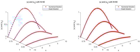
Figure 1.
and with for different N.
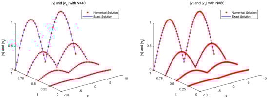
Figure 2.
and with for different N.
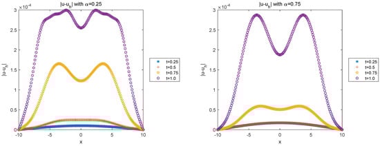
Figure 3.
with for different .
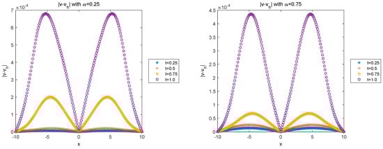
Figure 4.
with for different .
Example 2.
Consider the following two-dimensional nonlinear coupled time-fractional Schrödinger equations
where , and are determined by the exact solution pair and . The nonlinear term is selected as the following three cases []:
In Example 2, we test the convergence order of the proposed scheme by solving the two-dimensional nonlinear coupled fractional Schrödinger equations. For the convenience of calculation, we take the same space partition in both x and y directions. For the ease of description, we denote the numerical solution in Cases 1, 2, and 3 as , , and , respectively. The -errors and convergence rates with different and cases are listed in Table 2. We can observe again that the proposed scheme has an optimal convergence result with , and for three different nonlinear terms, all the convergence orders are close to 2. This shows that our scheme is effective for solving these nonlinear equations.
Table 2.
-errors and convergence rates of the proposed scheme with different for Cases 1–3.
To observe the approximation effect for different spatial parameters N on and , we separately plotted Figure 5 for and Figure 6 for of Case 1 with and the exact solution pair and at . In order to test the influence of time t, we draw the error graphs and of Case 2 with at different time points in Figure 7.
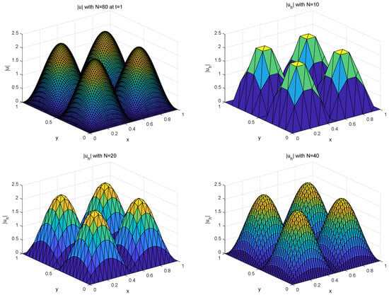
Figure 5.
and of Case 1 with for different N at .
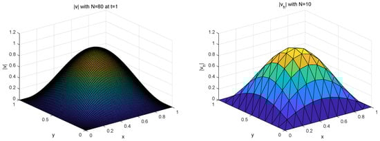
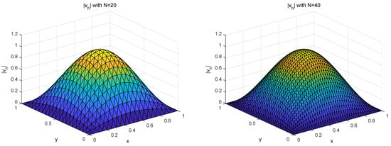
Figure 6.
and of Case 1 with for different N at .
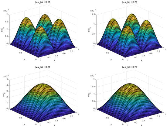
Figure 7.
and of Case 2 with at different t.
5. Conclusions and Advancements
In this article, to solve the nonlinear coupled time-fractional Schrödinger equations, we establish a fully discrete finite volume element method based on the formula. We provide the theoretical proof of stability, and derive the optimal error estimate. Finally, choosing several numerical examples, we carry out the numerical tests and obtain the approximate second-order convergence results, which are consistent with the theoretical optimal results, and indicate that the convergence is almost unaffected by the changed fractional parameter when the solution has good regularity.
In future work, we will continue to develop the finite volume element method for the coupled fractional Klein-Gordon-Schrödinger equations.
Author Contributions
X.Z.: methodology, validation, software, and writing—original draft preparation; Y.Y.: conceptualization, formal analysis, validation, and writing—review and editing; H.L.: validation, formal analysis, and writing—review and editing, funding acquisition; Z.F.: validation, formal analysis, and writing—review and editing; Y.L.: conceptualization, methodology, validation, formal analysis, funding acquisition, and writing—review and editing. All authors have read and agreed to the published version of the manuscript.
Funding
This work is supported by the Program for Innovative Research Team in Universities of Inner Mongolia Autonomous Region (NMGIRT2413, NMGIRT2207).
Data Availability Statement
All the data were computed using our algorithm. Data sharing is not applicable to this article as no dataset was generated or analyzed during the current study.
Conflicts of Interest
The authors declare no conflicts of interest.
References
- Hadhoud, A.R.; Agarwal, P.; Rageh, A.M. Numerical treatments of the nonlinear coupled time-fractional Schrödinger equations. Math. Meth. Appl. Sci. 2022, 45, 7119–7143. [Google Scholar] [CrossRef]
- Gao, W.; Li, H.; Liu, Y.; Wei, X.X. A Padé compact high-order finite volume scheme for nonlinear Schrödinger equations. Appl. Numer. Math. 2014, 85, 115–127. [Google Scholar] [CrossRef]
- Chen, C.J.; Lou, Y.Z.; Hu, H.Z. Two-grid finite volume element method for the time-dependent Schrödinger equation. Comput. Math. Appl. 2022, 108, 185–195. [Google Scholar] [CrossRef]
- Chen, C.J.; Lou, Y.Z.; Zhang, T. Two-grid Crank-Nicolson finite volume element method for the time-dependent Schrödinger equation. Adv. Appl. Math. Mech. 2022, 6, 1357–1380. [Google Scholar]
- Zhao, G.Y.; An, N.; Huang, C.B. Optimal error analysis of the Alikhanov formula for a time-fractional Schrödinger equation. J. Appl. Math. Comput. 2023, 69, 159–170. [Google Scholar] [CrossRef]
- Wang, Y.; Wang, G.; Bu, L.L.; Mei, L.Q. Two second-order and linear numerical schemes for the multi-dimensional nonlinear time-fractional Schrödinger equation. Numer. Algor. 2021, 88, 419–451. [Google Scholar] [CrossRef]
- Alikhanov, A.A. A new difference scheme for the time fractional diffusion equation. J. Comput. Phys. 2015, 280, 424–438. [Google Scholar] [CrossRef]
- Jia, J.Q.; Jiang, X.Y.; Zhang, H. An L1 Legendre-Galerkin spectral method with fast algorithm for the two-dimensional nonlinear coupled time fractional Schrödinger equation and its parameter estimation. Comput. Math. Appl. 2021, 82, 13–35. [Google Scholar] [CrossRef]
- Zhang, M.; Liu, F.; Turner, I.; Anh, V.; Feng, L. A finite volume method for the two-dimensional time and space variable-order fractional Bloch-Torrey equation with variable coefficients on irregular domains. Comput. Math. Appl. 2021, 98, 81–98. [Google Scholar] [CrossRef]
- Zhang, T.; Guo, Q.X. The finite difference/finite volume method for solving the fractional diffusion equation. J. Comput. Phys. 2018, 375, 120–134. [Google Scholar] [CrossRef]
- Fang, Z.C.; Zhao, J.; Li, H.; Liu, Y. Finite volume element methods for two-dimensional time fractional reaction-diffusion equations on triangular grids. Appl. Anal. 2023, 102, 2248–2270. [Google Scholar] [CrossRef]
- Fang, Z.C.; Zhao, J.; Li, H.; Liu, Y. A fast time two-mesh finite volume element algorithm for the nonlinear time-fractional coupled diffusion model. Numer. Algor. 2023, 93, 863–898. [Google Scholar] [CrossRef]
- Karaa, S.; Mustapha, K.; Pani, A. Finite volume element method for two-dimensional fractional subdiffusion problems. IMA J. Numer. Anal. 2017, 37, 945–964. [Google Scholar] [CrossRef]
- Richard, E.; Raytcho, L.; Lin, Y.P. Finite volume element approximations of nonlocal reactive flows in porous media. Numer. Meth. Part. Differ. Equ. 2000, 16, 285–311. [Google Scholar]
- Wang, X.; Huang, W.Z.; Li, Y.H. Conditioning of the finite volume element method for diffusion problems with general simplicial meshes. Math. Comput. 2019, 88, 2665–2696. [Google Scholar] [CrossRef]
- Wang, X.; Zhang, Y. On the construction and analysis of finite volume element schemes with optimal L2 convergence rate. Numer. Math. Theor. Meth. Appl. 2021, 14, 47–70. [Google Scholar]
- Gao, G.H.; Alikhanov, A.A.; Sun, Z.Z. The temporal second order difference schemes based on the interpolation approximation for solving the time multi-term and distributed-order fractional sub-diffusion equations. J. Sci. Comput. 2017, 73, 93–121. [Google Scholar] [CrossRef]
- Wang, J.F.; Yin, B.L.; Liu, Y.; Li, H.; Fang, Z.C. Mixed finite element algorithm for a nonlinear time fractional wave model. Math. Comput. Simulat. 2021, 188, 60–76. [Google Scholar] [CrossRef]
- Qin, H.Y.; Wu, F.Y.; Zhou, B.Y. Alikhanov linearized Galerkin finite element methods for nonlinear time-fractional Schrödinger equations. J. Comput. Math. 2023, 41, 1305–1324. [Google Scholar] [CrossRef]
- Liu, J.F.; Wang, T.C.; Zhang, T. A second-order finite difference scheme for the multi-dimensional nonlinear time-fractional Schrödinger equation. Numer. Algor. 2023, 92, 1153–1182. [Google Scholar] [CrossRef]
- Li, R.H.; Chen, Z.; Wu, W. Generalized Difference Methods for Differential Equations: Numerical Analysis of Finite Volume Methods; CRC Press: Boca Raton, FL, USA, 2000. [Google Scholar]
- Liao, H.L.; William, M.; Zhang, J.W. A discrete Grönwall inequality with application to numerical schemes for subdiffusion problems. SIAM J. Numer. Anal. 2019, 57, 218–237. [Google Scholar] [CrossRef]
Disclaimer/Publisher’s Note: The statements, opinions and data contained in all publications are solely those of the individual author(s) and contributor(s) and not of MDPI and/or the editor(s). MDPI and/or the editor(s) disclaim responsibility for any injury to people or property resulting from any ideas, methods, instructions or products referred to in the content. |
© 2024 by the authors. Licensee MDPI, Basel, Switzerland. This article is an open access article distributed under the terms and conditions of the Creative Commons Attribution (CC BY) license (https://creativecommons.org/licenses/by/4.0/).