Dynamics of the Traveling Wave Solutions of Fractional Date–Jimbo–Kashiwara–Miwa Equation via Riccati–Bernoulli Sub-ODE Method through Bäcklund Transformation

Abstract

The dynamical wave solutions of the time–space fractional Date–Jimbo–Kashiwara–Miwa (DJKM) equation have been obtained in this article using an innovative and efficient technique including the Riccati–Bernoulli sub-ODE method through Bäcklund transformation. Fractional-order derivatives enter into play for their novel contribution to the enhancement of the characterization of dynamic waves while providing better modeling ability compared to integer types of derivatives. The solutions of the above-mentioned time–space fractional Date–Jimbo–Kashiwara–Miwa equation have tremendous importance in numerous scientific scenarios. The regular dynamical wave solutions of the aforementioned equation encompass three fundamental functions: trigonometric, hyperbolic, and rational functions will be among the topics covered. These solutions are graphically classified into three categories: compacton kink solitary wave solutions, kink soliton wave solutions and anti-kink soliton wave solutions. In addition, to explore the impact of the fractional parameter ($\alpha$) on those solutions, $2D$ plots are utilized, while $3D$ plots are applied to present the solutions involving the integer-order derivatives.

1. Introduction

It is established that fractional-order derivatives provide a remarkable way of describing the wave dynamics because of more flexibility in terms of frequency and phase responses than the integer ones, which do not consider the memory and hereditary nature of the wave systems adequately. With the use of fractional derivatives, it becomes possible to also take into consideration non-locality interactions and anomalous diffusion, thus improving the precision in wave dynamics and propagation. This approach enhances the capacity to give and analyze details of wave complex structures, making the application of this approach key to enhancing the understanding of complex structures. A wide range of phenomena can be described by partial differential equations that are referred to as quasi-linear or nonlinear evolution equations (NLEEs). These are mathematical equations that are dependent on space and time, and they can practically replicate virtually all the phenomena in the natural world, mainly in the science and engineering industries. For depicting the phenomena in the various sectors of science like engineering, solid-state physics, plasma physics, applied physics, applied mathematics, plasma waves, fluid mechanics, quantum mechanics, electrodynamics, magnetohydrodynamics, turbulence, biology, fiberoptics, chemistry, chemical physics, astrophysics, theory of relativity, cosmology and medical science, it becomes relevant to look for exact solutions of NLEEs [1,2,3,4,5]. Numerous researchers have developed various methods to obtain exact solutions for NLEEs. These include the lie group method, the $exp(-\varphi (x\left)\right)$-expansion method, the extended direct algebraic method, the variational iteration method, the unified method, the $(G^{\prime }/G^2)$–expansion method, the sine–gordon expansion method, the tanh–coth method, the homotopy analysis method, the auxiliary ordinary differential equation method, and the tanh function method [6,7,8,9,10]. Moreover, applications of fractional calculus (FC) have increased extensively in different branches of science and engineering. It has been used to model and predict many high-order algorithms and nonlinear mechanics of physics and applied electromagnetism and engineering or anomalous diffusion, chemical kinetics, viscoelasticity, and electrochemistry, and so on [11,12,13,14,15,16]. The application of fractional calculus has been on the rise in these fields in the last few decades. Many algorithms have been proposed for handling nonlinear FDEs, which implies the significance and versatility of FC in expanding the existing understanding and capacity for analyzing and modeling systems [17,18,19]. As evident from the above discussion, the improvement of techniques regarding the FDEs has enabled researchers to solve the problems which were previously beyond the scope of any theoretical and computational tool, leading to numerous new insights and ideas in various scientific and engineering fields. One of the most interesting and intricate cases of usage of fractional calculus is related to the solution of various partial differential equations using different types of fractional derivatives that are both numerical and analytical [20,21,22,23,24].

The Kadomtsev–Petviashil (KP) equation is one of the essential equations for solitons and is crucial for the connection between mathematics and physics. The Date–Jimbo–Kashiwara–Miwa (DJKM) equation, a member of the KP hierarchy equations, can be expressed as follows [25,26]:

$$D_y^{\alpha }\left(D_x^{3\alpha }f\right)+4D_y^{\alpha }\left(D_x^{2\alpha }f\right)D_x^{\alpha }f+\left(2D_x^{3\alpha }f\right)D_y^{\alpha }f+6D_y^{\alpha }\left(D_x^{\alpha }f\right)\left(D_x^{2\alpha }f\right)-\lambda \left(D_y^{3\alpha }f\right)-2\gamma D_t^{\alpha }\left(D_x^{2\alpha }f\right)=0.$$

(1)

Here, the notation $f(x,y,t)$ is used for the wave amplitude, with (t) being the time variable. According to the said parameter, the parameter ( $0<\alpha \le 1$) refers to the fractal dimensions related to the time (t) and the spatial coordinates ($x,y$). Further, the operator integrating $\alpha$-derivatives of powers agree exactly with the idea of conformable fractional derivatives [17].

$$\begin{array}{c}\hfill D_{\Theta }^{\alpha }M(\Theta )=\underset{i\to 0}{lim}{\displaystyle \frac{M(i{(\Theta )}^{i-\alpha }-M\left(\theta \right))}{i}},0<\alpha \le 1.\end{array}$$

(2)

$$\left\{\begin{array}{c}{D}_{\Theta }^{\alpha }{\Theta }^m=m{\Theta }^{m-\alpha }.\hfill \\ D_{\Theta }^{\alpha }\left(m_1\eta (\Theta )\pm m_{2}t(\Theta )\right)=m_1{D}_{\Theta }^{\alpha }\left(\eta (\Theta )\right)\pm m_2{D}_{\Theta }^{\alpha }\left(t(\Theta )\right).\hfill \\ D_{\Theta }^{\alpha }\left[f\circ g\right]={\Theta }^{1-\alpha }g\left(\Theta \right)D_{\Theta }^{\alpha }f\left(g(\Theta )\right).\hfill \end{array}\right.$$

(3)

The (DJKM) equation describes long water waves using frequency dispersion and nonlinear restoring forces that are considered to be weak. This equation has been analyzed with the help of a number of powerful methods among which it is possible to mention the Hirota bilinear method [25], the extended transformed rational function method [27], and the Wronskian and Grammian techniques [28]. Wazwaz [26] proved that this equation is Painleve integrable and obtained several soliton solutions of the (2+1)-dimensional DJKM equation. In this work, the method of Ricatti–Bernoulli sub–ODE will be used to obtain analytical solutions for the (DJKM) equation. This will be accomplished by using the proposed approach [29,30,31] and the Bäcklund transformation with respect to nonlinear wave effects. This paper is structured as follows:

In Section 2, a brief description of the used methods is provided. Section 3 indicates the actual solutions of the fractional (DJKM) equation. Section 4 focuses on results and discussion and providing graphical illustrations. In the last section, Section 5, the conclusion of our work is provided.

2. Algorithm

Consider the nonlinear partial differential equation of the following form:

$$p_1\left(U,D_t^{\alpha }\left(U\right),D_{x_1}^{\alpha }\left(U\right),D_{x_2}^{\alpha }\left(U\right),U{D}_{x_1}^{\alpha }\left(U\right),\dots \right)=0,0<\alpha \le 1,$$

(4)

where $U=U(t,x_1,x_2,x_3,\dots ,x_k)$ is an unknown function and $p_1$ is a polynomial in U and its partial derivatives. We use the wave transformation to translate Equation (4) into an ordinary differential equation (ODE) of the following form:

$$V(\Phi )=v(t,x_1,x_2,x_3,\dots ,x_k),\Phi =a{\displaystyle \frac{t^{\alpha }}{\alpha }}+b{\displaystyle \frac{x_1^{\alpha }}{\alpha }}+c{\displaystyle \frac{x_2^{\alpha }}{\alpha }}+\dots ,+\omega {\displaystyle \frac{x_k^{\alpha }}{\alpha }},$$

(5)

where ($\omega$) is the traveling wave velocity and (a), (b), are constants. It follows that Equation (4) becomes an ordinary differential equation:

$$p_2\left(V,V^{\prime }(\Phi ),V^{″}(\Phi ),V{V}^{\prime }(\Phi ),\dots \right)=0,$$

(6)

Equation (6), a wave solution, is expressed as a finite series using the proposed approach:

$$G(\Phi )=\sum _{i=-n}^n{k}_i{g(\Phi )}^i,$$

(7)

In this work, focus is made on the change of $g=g(\Phi )$ as described through the Bäcklund transformation. The Bäcklund transformation can be used as a tool when solving nonlinear differential equations. Specifically, the function (g) as a function of ($\Phi$) is articulated through the following Bäcklund transformation framework:

$$g(\Phi )={\displaystyle \frac{-\rho Y_2+Y_{1}Z(\Phi )}{Y_1+Y_{2}Z(\Phi )}},$$

(8)

where ($\rho$), ($Y_1$), and ($Y_2$) are constants such that $Y_2\ne 0$ and $Z=Z(\Phi )$ represent a solution to the generalized Ricatti equation:

$${\displaystyle \frac{dZ}{d\Phi }}=\rho +Z{(\Phi )}^2.$$

(9)

The Ricatti Equation (9) possess the following general solutions [32].

$$\begin{array}{cc}\hfill & Z(\Phi )=\left\{\begin{array}{cc}-\sqrt{-\rho }tanh(\sqrt{-\rho }\Phi ),\hfill & \mathrm{as}\rho <0,\hfill \\ -\sqrt{-\rho }coth(\sqrt{-\rho }\Phi ),\hfill & \mathrm{as}\rho <0,\hfill \end{array}\right.\hfill \\ \hfill & Z(\Phi )=-{\displaystyle \frac{1}{\Phi }},\mathrm{as}\rho =0,\hfill \\ \hfill & Z(\Phi )=\left\{\begin{array}{cc}\sqrt{\rho }tan(\sqrt{\rho }\Phi ),\hfill & \mathrm{as}\rho >0,\hfill \\ -\sqrt{\rho }cot(\sqrt{\rho }\Phi ),\hfill & \mathrm{as}\rho >0.\hfill \end{array}\right.\hfill \end{array}$$

(10)

The next step is to obtain the positive integer (n) in our assumed solution by comparing the orders of derivative terms and nonlinear terms for ordinary differential equations. Plug the proposed solution and convert this into a system of algebraic equations and set the coefficients of $Z(\Phi )$ to zero. Then, we plugged the constants ($k_i$), ($\omega$), and ($\rho$) we obtained earlier into that algebraic equation which is derived from expansion of functions and solved them in Maple. Consequently, we obtained a set of exact solutions for Equation (4).

3. Problem Execution

This section deals with a new a new algorithm in order to solve the space–time fractional (DJKM) equation, which describes long waves affected by frequency dispersion and weak nonlinear restoring forces. Here, one of the principal aims is to obtain an analytic soliton solution for this fractional partial differential equation (PDE). This is an evaluation of $f(x,y,t)$ at a retarded time (t) due to the propagation in (x). In order to carry this out, we need the wave transformation which transforms Equation (1) into an ordinary differential equation (ODE), making it easier for us deal with them analytically.

$$\begin{array}{c}\hfill f(x,y,t)=F(\Phi ),\mathrm{where}\Phi ={\displaystyle \frac{p{x}^{\alpha }}{\alpha }}+{\displaystyle \frac{q{y}^{\alpha }}{\alpha }}-{\displaystyle \frac{\omega t^{\alpha }}{\alpha }}.\end{array}$$

(11)

where (p), (q), and ($\omega$) are constants. Applying the above wave transformation, we convert Equation (1) into a nonlinear ordinary differential equation (ODE):

$$\begin{array}{c}\hfill 6p^{3}q{\left({\displaystyle \frac{d^{2}F}{d{\Phi }^2}}\right)}^2-q^3\lambda \left({\displaystyle \frac{d^{3}F}{d{\Phi }^3}}\right)+2p^2\omega \gamma \left({\displaystyle \frac{d^{3}F}{d{\Phi }^3}}\right)+6p^{3}q\left({\displaystyle \frac{d^{3}F}{d{\Phi }^3}}\right)\left({\displaystyle \frac{dF}{d\Phi }}\right)+p^{4}q\left({\displaystyle \frac{d^{5}F}{d{\Phi }^5}}\right)=0.\end{array}$$

(12)

Now, after integrating Equation (12) and keeping the constant of integration zero for simplicity, we have

$$-q^3\lambda \left({\displaystyle \frac{d^{2}F}{d{\Phi }^2}}\right)+2p^2\omega \gamma \left({\displaystyle \frac{d^{2}F}{d{\Phi }^2}}\right)+6p^{3}q\left({\displaystyle \frac{d^{2}F}{d{\Phi }^2}}\right)\left({\displaystyle \frac{dF}{d\Phi }}\right)+p^{4}q\left({\displaystyle \frac{d^{4}F}{d{\Phi }^4}}\right)=0.$$

(13)

Balancing ($F^{″″}$) and $F^{\prime }{F}^{″}$, we obtain N = 1 [33]. Substituting Equation (7) with Equation (9) into Equation (13) and then collecting the coefficients of $Z{(\Phi )}^i$ yields the following system:

$$\begin{array}{cc}\hfill & 24p^{4}q{k}_1{Y_2}^{10}{\rho }^{10}+12p^{3}q{k_1}^2{Y_2}^{10}{\rho }^{10}=0,\hfill \\ \hfill & 40p^{4}q{k}_1{Y_2}^{10}{\rho }^9-2q^3\lambda k_1{Y_2}^{10}{\rho }^8+24p^{3}q{k_1}^2{Y_2}^{10}{\rho }^9+4p^2\omega \gamma k_1{Y_2}^{10}{\rho }^8-12p^{3}q{k}_{-1}{Y_2}^{10}{\rho }^8{k}_1=0,\hfill \\ \hfill & -2q^3\lambda k_1{Y_2}^{10}{\rho }^7+16p^{4}q{k}_1{Y_2}^{10}{\rho }^8+12p^{3}q{k_1}^2{Y_2}^{10}{\rho }^8+4p^2\omega \gamma k_1{Y_2}^{10}{\rho }^7-12p^{3}q{k}_{-1}{Y_2}^{10}{\rho }^7{k}_1=0,\hfill \\ \hfill & -2q^3\lambda k_{-1}{Y_2}^{10}{\rho }^5+16p^{4}q{k}_{-1}{Y_2}^{10}{\rho }^6-12p^{3}q{k_{-1}}^2{Y_2}^{10}{\rho }^5+12p^{3}q{k}_{-1}{Y_2}^{10}{\rho }^6{k}_1+4p^2\omega \gamma k_{-1}{Y_2}^{10}{\rho }^5=0,\hfill \\ \hfill & 40p^{4}q{k}_{-1}{Y_2}^{10}{\rho }^5-24p^{3}q{k_{-1}}^2{Y_2}^{10}{\rho }^4-2q^3\lambda k_{-1}{Y_2}^{10}{\rho }^4+12p^{3}q{k}_{-1}{Y_2}^{10}{k}_1{\rho }^5+4p^2\omega \gamma k_{-1}{Y_2}^{10}{\rho }^4=0,\hfill \\ \hfill & 24p^{4}q{k}_{-1}{Y_2}^{10}{\rho }^4-12p^{3}q{k_{-1}}^2{Y_2}^{10}{\rho }^3=0.\hfill \end{array}$$

(14)

This give us the algebraic equations by setting $Z(\Phi )=0$. The solutions of this system of algebraic equations obtained from Maple are below:

Set:1

$$\begin{array}{c}\hfill k_0=k_0,k_1=0,k_{-1}=1/2{\displaystyle \frac{-q^3\lambda +2p^2\omega \gamma }{p^{3}q}},\rho =1/4{\displaystyle \frac{-q^3\lambda +2p^2\omega \gamma }{p^{4}q}},\omega =\omega ,p=p,q=q.\end{array}$$

(15)

Set:2

$$\begin{array}{c}\hfill k_0=k_0,k_1=-2p,k_{-1}=0,\rho =1/4{\displaystyle \frac{-q^3\lambda +2p^2\omega \gamma }{p^{4}q}},\omega =\omega ,p=p,q=q.\end{array}$$

(16)

Set:3

$$\begin{array}{c}\hfill k_0=k_0,k_1=-2p,k_{-1}=1/8{\displaystyle \frac{-q^3\lambda +2p^2\omega \gamma }{p^{3}q}},\rho =1/16{\displaystyle \frac{-q^3\lambda +2p^2\omega \gamma }{p^{4}q}},\omega =\omega ,p=p,q=q.\end{array}$$

(17)

3.1. Solution Set 1

For Equation (1), we obtain the following set of solutions (when $\rho <0$), and for this, we consider set 1.

$$\begin{array}{cc}\hfill & f_1(x,y,t)=1/2\left(-q^3\lambda +2p^2\omega \gamma \right)\left(Y_1-1/2Y_2\sqrt{-{\displaystyle \frac{-q^3\lambda +2p^2\omega \gamma }{p^{4}q}}}tanh\left(1/2\sqrt{-{\displaystyle \frac{-q^3\lambda +2p^2\omega \gamma }{p^{4}q}}}\Phi \right)\right)\hfill \\ \hfill & p^{-3}{q}^{-1}{\left(-1/4{\displaystyle \frac{\left(-q^3\lambda +2p^2\omega \gamma \right)Y_2}{p^{4}q}}-1/2Y_1\sqrt{-{\displaystyle \frac{-q^3\lambda +2p^2\omega \gamma }{p^{4}q}}}tanh\left(1/2\sqrt{-{\displaystyle \frac{-q^3\lambda +2p^2\omega \gamma }{p^{4}q}}}\Phi \right)\right)}^{-1}+k_0.\hfill \end{array}$$

(18)

or

$$\begin{array}{cc}\hfill & f_2(x,y,t)=1/2\left(-q^3\lambda +2p^2\omega \gamma \right)\left(Y_1-1/2Y_2\sqrt{-{\displaystyle \frac{-q^3\lambda +2p^2\omega \gamma }{p^{4}q}}}coth\left(1/2\sqrt{-{\displaystyle \frac{-q^3\lambda +2p^2\omega \gamma }{p^{4}q}}}\Phi \right)\right)\hfill \\ \hfill & p^{-3}{q}^{-1}{\left(-1/4{\displaystyle \frac{\left(-q^3\lambda +2p^2\omega \gamma \right)Y_2}{p^{4}q}}-1/2Y_1\sqrt{-{\displaystyle \frac{-q^3\lambda +2p^2\omega \gamma }{p^{4}q}}}coth\left(1/2\sqrt{-{\displaystyle \frac{-q^3\lambda +2p^2\omega \gamma }{p^{4}q}}}\Phi \right)\right)}^{-1}+k_0.\hfill \end{array}$$

(19)

3.2. Solution Set 2

For Equation (1), we obtain the following set of solutions (when $\rho >0$), and for this, we consider set 1.

$$\begin{array}{cc}\hfill & f_3(x,y,t)=1/2\left(-q^3\lambda +2p^2\omega \gamma \right)\left(Y_1+1/2Y_2\sqrt{{\displaystyle \frac{-q^3\lambda +2p^2\omega \gamma }{p^{4}q}}}tan\left(1/2\sqrt{{\displaystyle \frac{-q^3\lambda +2p^2\omega \gamma }{p^{4}q}}}\Phi \right)\right)\hfill \\ \hfill & p^{-3}{q}^{-1}{\left(-1/4{\displaystyle \frac{\left(-q^3\lambda +2p^2\omega \gamma \right)Y_2}{p^{4}q}}+1/2Y_1\sqrt{{\displaystyle \frac{-q^3\lambda +2p^2\omega \gamma }{p^{4}q}}}tan\left(1/2\sqrt{{\displaystyle \frac{-q^3\lambda +2p^2\omega \gamma }{p^{4}q}}}\Phi \right)\right)}^{-1}+k_0.\hfill \end{array}$$

(20)

or

$$\begin{array}{cc}\hfill & f_4(x,y,t)=1/2\left(-q^3\lambda +2p^2\omega \gamma \right)\left(Y_1-1/2Y_2\sqrt{{\displaystyle \frac{-q^3\lambda +2p^2\omega \gamma }{p^{4}q}}}cot\left(1/2\sqrt{{\displaystyle \frac{-q^3\lambda +2p^2\omega \gamma }{p^{4}q}}}\Phi \right)\right)\hfill \\ \hfill & p^{-3}{q}^{-1}{\left(-1/4{\displaystyle \frac{\left(-q^3\lambda +2p^2\omega \gamma \right)Y_2}{p^{4}q}}-1/2Y_1\sqrt{{\displaystyle \frac{-q^3\lambda +2p^2\omega \gamma }{p^{4}q}}}cot\left(1/2\sqrt{{\displaystyle \frac{-q^3\lambda +2p^2\omega \gamma }{p^{4}q}}}\Phi \right)\right)}^{-1}+k_0.\hfill \end{array}$$

(21)

3.3. Solution Set 3

For Equation (1), we obtain the following set of solutions (when $\rho =0$), and for this, we consider set 1.

$$\begin{array}{cc}\hfill & f_5(x,y,t)=1/2\left(-q^3\lambda +2p^2\omega \gamma \right)\left(Y_1-{\displaystyle \frac{Y_2}{\Phi }}\right)p^{-3}{q}^{-1}{\left(-1/4{\displaystyle \frac{\left(-q^3\lambda +2p^2\omega \gamma \right)Y_2}{p^{4}q}}-{\displaystyle \frac{Y_1}{\Phi }}\right)}^{-1}+k_0.\hfill \end{array}$$

(22)

where, $\Phi ={\displaystyle \frac{p{x}^{\alpha }}{\alpha }}+{\displaystyle \frac{q{y}^{\alpha }}{\alpha }}-{\displaystyle \frac{\omega t^{\alpha }}{\alpha }}.$

3.4. Solution Set 4

For Equation (1), we obtain the following set of solutions (when $\rho <0$), and for this, we consider set 2.

$$\begin{array}{cc}\hfill f_6(x,y,t)=& k_0-2p\left(-1/4{\displaystyle \frac{\left(-q^3\lambda +2p^2\omega \gamma \right)Y_2}{p^{4}q}}-1/2Y_1\sqrt{-{\displaystyle \frac{-q^3\lambda +2p^2\omega \gamma }{p^{4}q}}}tanh\left(1/2\sqrt{-{\displaystyle \frac{-q^3\lambda +2p^2\omega \gamma }{p^{4}q}}}\Phi \right)\right)\hfill \\ \hfill & {\left(Y_1-1/2Y_2\sqrt{-{\displaystyle \frac{-q^3\lambda +2p^2\omega \gamma }{p^{4}q}}}tanh\left(1/2\sqrt{-{\displaystyle \frac{-q^3\lambda +2p^2\omega \gamma }{p^{4}q}}}\Phi \right)\right)}^{-1}.\hfill \end{array}$$

(23)

or

$$\begin{array}{cc}\hfill f_7(x,y,t)=& k_0-2p\left(-1/4{\displaystyle \frac{\left(-q^3\lambda +2p^2\omega \gamma \right)Y_2}{p^{4}q}}-1/2Y_1\sqrt{-{\displaystyle \frac{-q^3\lambda +2p^2\omega \gamma }{p^{4}q}}}coth\left(1/2\sqrt{-{\displaystyle \frac{-q^3\lambda +2p^2\omega \gamma }{p^{4}q}}}\Phi \right)\right)\hfill \\ \hfill & {\left(Y_1-1/2Y_2\sqrt{-{\displaystyle \frac{-q^3\lambda +2p^2\omega \gamma }{p^{4}q}}}coth\left(1/2\sqrt{-{\displaystyle \frac{-q^3\lambda +2p^2\omega \gamma }{p^{4}q}}}\Phi \right)\right)}^{-1}.\hfill \end{array}$$

(24)

3.5. Solution Set 5

For Equation (1), we obtain the following set of solutions (when $\rho >0$), and for this, we consider set 2.

$$\begin{array}{cc}\hfill f_8(x,y,t)=& k_0-2p\left(-1/4{\displaystyle \frac{\left(-q^3\lambda +2p^2\omega \gamma \right)Y_2}{p^{4}q}}+1/2Y_1\sqrt{{\displaystyle \frac{-q^3\lambda +2p^2\omega \gamma }{p^{4}q}}}tan\left(1/2\sqrt{{\displaystyle \frac{-q^3\lambda +2p^2\omega \gamma }{p^{4}q}}}\Phi \right)\right)\hfill \\ \hfill & {\left(Y_1+1/2Y_2\sqrt{{\displaystyle \frac{-q^3\lambda +2p^2\omega \gamma }{p^{4}q}}}tan\left(1/2\sqrt{{\displaystyle \frac{-q^3\lambda +2p^2\omega \gamma }{p^{4}q}}}\Phi \right)\right)}^{-1}.\hfill \end{array}$$

(25)

or

$$\begin{array}{cc}\hfill f_9(x,y,t)=& k_0-2p\left(-1/4{\displaystyle \frac{\left(-q^3\lambda +2p^2\omega \gamma \right)Y_2}{p^{4}q}}-1/2Y_1\sqrt{{\displaystyle \frac{-q^3\lambda +2p^2\omega \gamma }{p^{4}q}}}cot\left(1/2\sqrt{{\displaystyle \frac{-q^3\lambda +2p^2\omega \gamma }{p^{4}q}}}\Phi \right)\right)\hfill \\ \hfill & {\left(Y_1-1/2Y_2\sqrt{{\displaystyle \frac{-q^3\lambda +2p^2\omega \gamma }{p^{4}q}}}cot\left(1/2\sqrt{{\displaystyle \frac{-q^3\lambda +2p^2\omega \gamma }{p^{4}q}}}\Phi \right)\right)}^{-1}.\hfill \end{array}$$

(26)

3.6. Solution Set 6

For Equation (1), we obtain the following set of solutions (when ($\rho =0$), and for this, we consider set 2.

$$\begin{array}{c}\hfill f_{10}(x,y,t)=k_0-2p\left(-1/4{\displaystyle \frac{\left(-q^3\lambda +2p^2\omega \gamma \right)Y_2}{p^{4}q}}-{\displaystyle \frac{Y_1}{\Phi }}\right){\left(Y_1-{\displaystyle \frac{Y_2}{\Phi }}\right)}^{-1}.\end{array}$$

(27)

where, $\Phi ={\displaystyle \frac{p{x}^{\alpha }}{\alpha }}+{\displaystyle \frac{q{y}^{\alpha }}{\alpha }}-{\displaystyle \frac{\omega t^{\alpha }}{\alpha }}.$

3.7. Solution Set 7

For Equation (1), we obtain the following set of solutions (when $\rho <0$), and for this, we consider set 3.

$$\begin{array}{c}\hfill f_{11}(x,y,t)=1/8{\displaystyle \frac{\left(-q^3\lambda +2p^2\omega \gamma \right)\left(Y_1-Y_2\sqrt{-\rho }tanh\left(\sqrt{-\rho }\Phi \right)\right)}{p^{3}q\left(-\rho Y_2-Y_1\sqrt{-\rho }tanh\left(\sqrt{-\rho }\Phi \right)\right)}}+k_0-2{\displaystyle \frac{p\left(-\rho Y_2-Y_1\sqrt{-\rho }tanh\left(\sqrt{-\rho }\Phi \right)\right)}{Y_1-Y_2\sqrt{-\rho }tanh\left(\sqrt{-\rho }\Phi \right)}}.\end{array}$$

(28)

or

$$\begin{array}{c}\hfill f_{12}(x,y,t)=1/8{\displaystyle \frac{\left(-q^3\lambda +2p^2\omega \gamma \right)\left(Y_1-Y_2\sqrt{-\rho }coth\left(\sqrt{-\rho }\Phi \right)\right)}{p^{3}q\left(-\rho Y_2-Y_1\sqrt{-\rho }coth\left(\sqrt{-\rho }\Phi \right)\right)}}+k_0-2{\displaystyle \frac{p\left(-\rho Y_2-Y_1\sqrt{-\rho }coth\left(\sqrt{-\rho }\Phi \right)\right)}{Y_1-Y_2\sqrt{-\rho }coth\left(\sqrt{-\rho }\Phi \right)}}.\end{array}$$

(29)

3.8. Solution Set 8

For Equation (1), we obtain the following set of solutions (when $\rho >0$), and for this, we consider set 3.

$$\begin{array}{c}\hfill f_{13}(x,y,t)=1/8{\displaystyle \frac{\left(-q^3\lambda +2p^2\omega \gamma \right)\left(Y_1+Y_2\sqrt{\rho }tan\left(\sqrt{\rho }\Phi \right)\right)}{p^{3}q\left(-\rho Y_2+Y_1\sqrt{\rho }tan\left(\sqrt{\rho }\Phi \right)\right)}}+k_0-2{\displaystyle \frac{p\left(-\rho Y_2+Y_1\sqrt{\rho }tan\left(\sqrt{\rho }\Phi \right)\right)}{Y_1+Y_2\sqrt{\rho }tan\left(\sqrt{\rho }\Phi \right)}}.\end{array}$$

(30)

or

$$\begin{array}{c}\hfill f_{14}(x,y,t)=1/8{\displaystyle \frac{\left(-q^3\lambda +2p^2\omega \gamma \right)\left(Y_1-Y_2\sqrt{\rho }cot\left(\sqrt{\rho }\Phi \right)\right)}{p^{3}q\left(-\rho Y_2-Y_1\sqrt{\rho }cot\left(\sqrt{\rho }\Phi \right)\right)}}+k_0-2{\displaystyle \frac{p\left(-\rho Y_2-Y_1\sqrt{\rho }cot\left(\sqrt{\rho }\Phi \right)\right)}{Y_1-Y_2\sqrt{\rho }cot\left(\sqrt{\rho }\Phi \right)}}.\end{array}$$

(31)

3.9. Solution Set 9

For Equation (1), we obtain the following set of solutions (when $\rho =0$), and for this, we consider set 3.

$$\begin{array}{c}\hfill f_{15}(x,y,t)=1/8\left(-q^3\lambda +2p^2\omega \gamma \right)\left(Y_1-{\displaystyle \frac{Y_2}{\Phi }}\right)p^{-3}{q}^{-1}{\left(-\rho Y_2-{\displaystyle \frac{Y_1}{\Phi }}\right)}^{-1}+k_0-2p\left(-\rho Y_2-{\displaystyle \frac{Y_1}{\Phi }}\right){\left(Y_1-{\displaystyle \frac{Y_2}{\Phi }}\right)}^{-1}.\end{array}$$

(32)

where $\rho =1/16{\displaystyle \frac{-q^3\lambda +2p^2\omega \gamma }{p^{4}q}}$ and $\Phi ={\displaystyle \frac{p{x}^{\alpha }}{\alpha }}+{\displaystyle \frac{q{y}^{\alpha }}{\alpha }}-{\displaystyle \frac{\omega t^{\alpha }}{\alpha }}.$

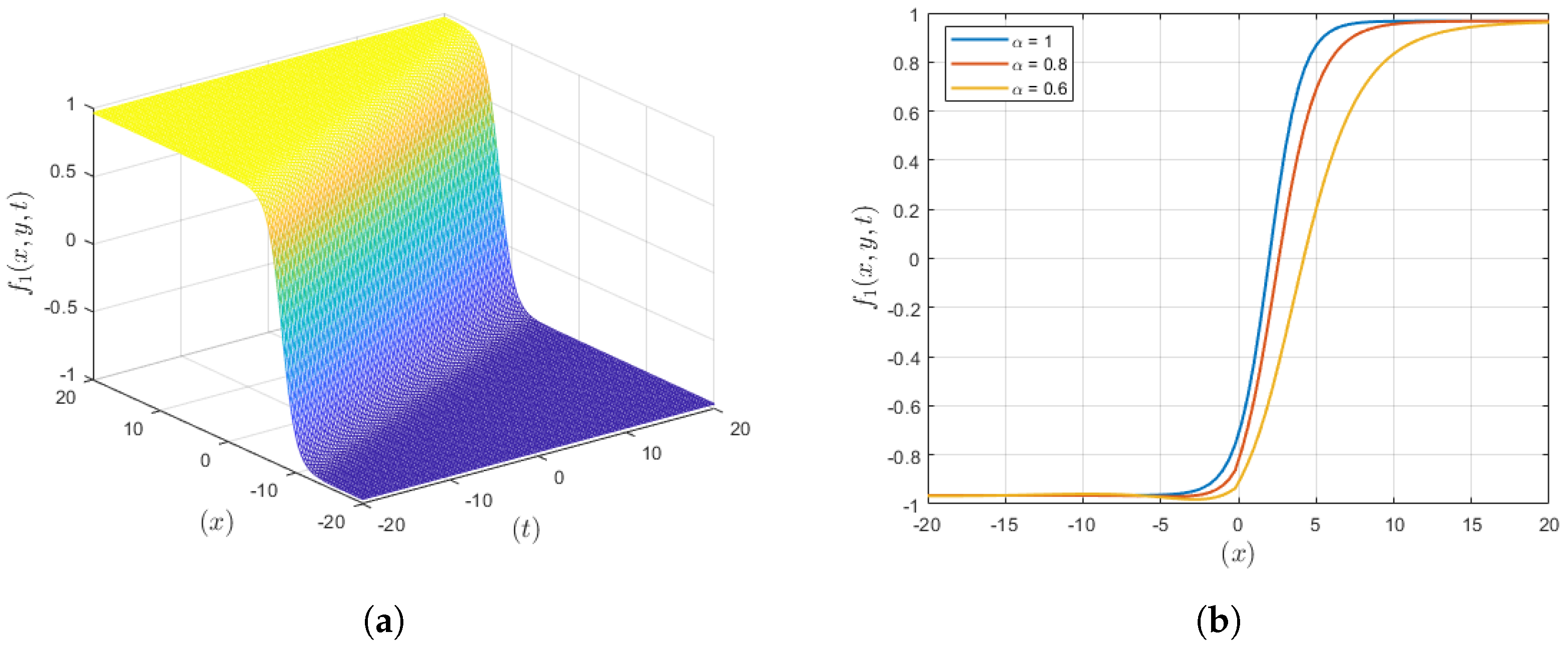
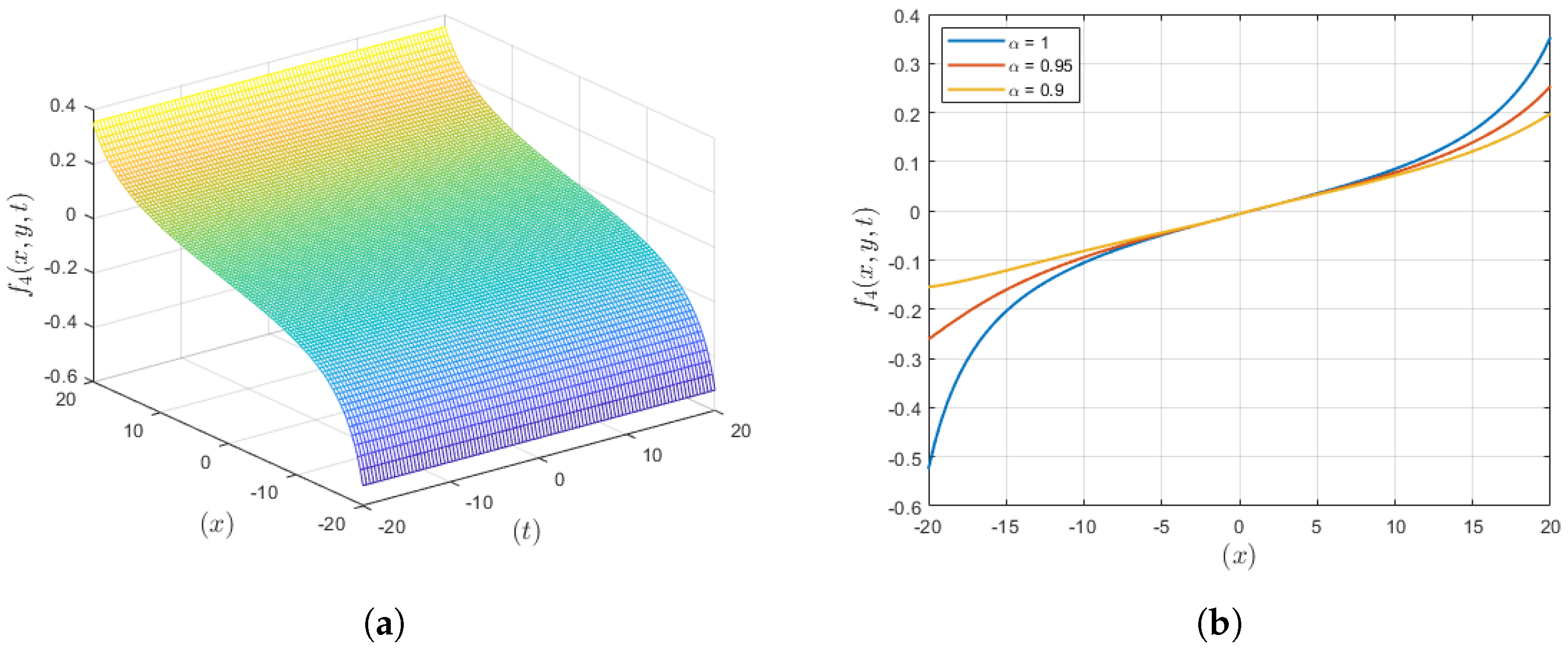
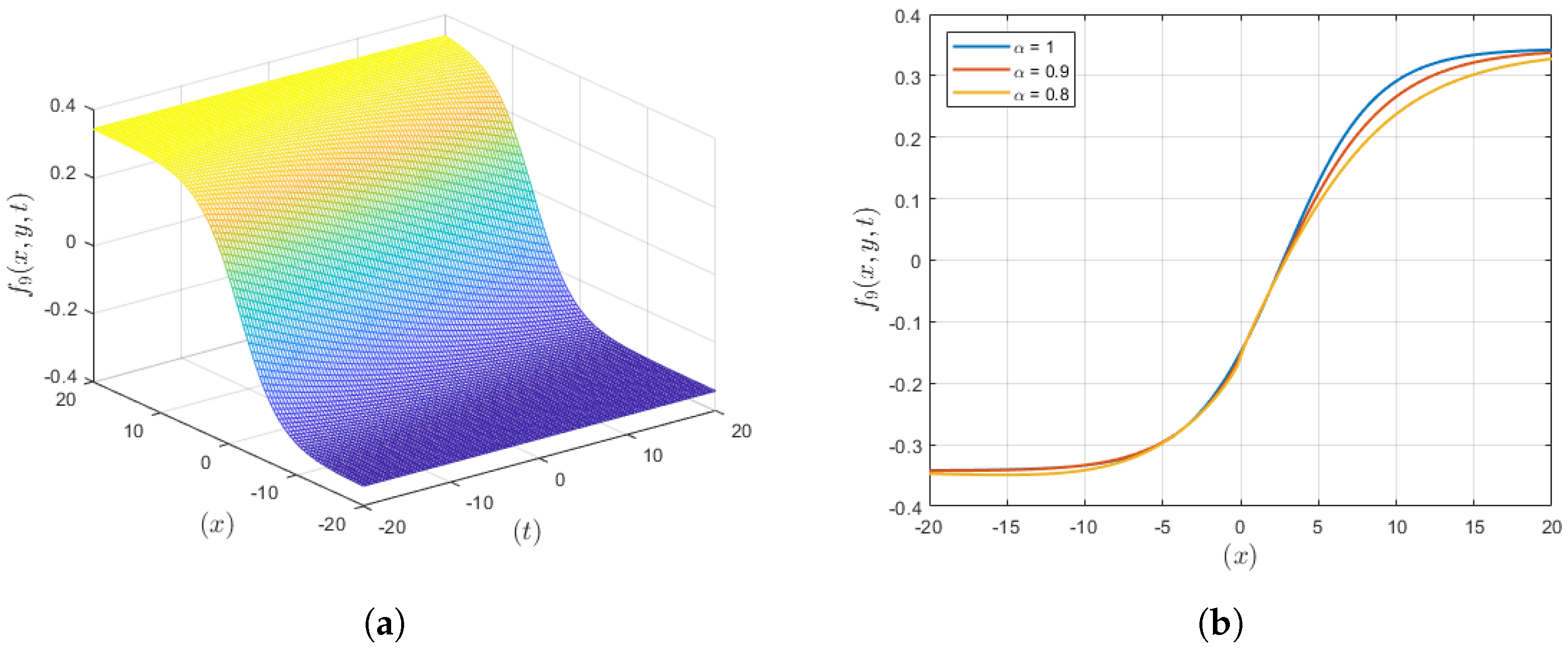
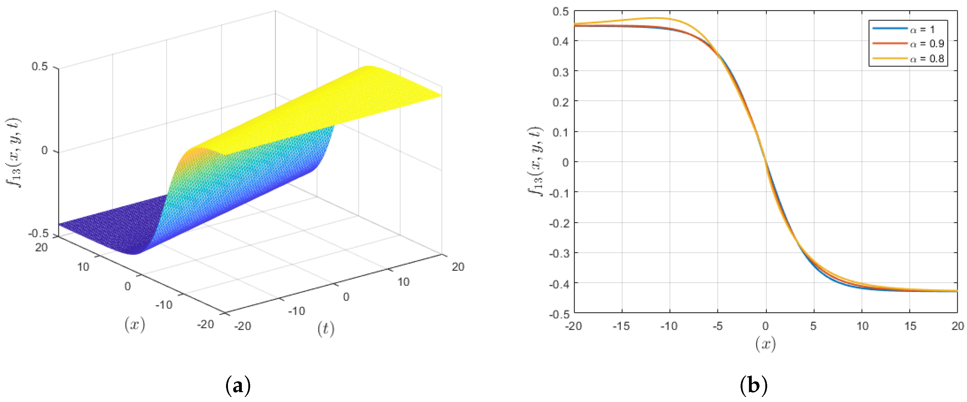
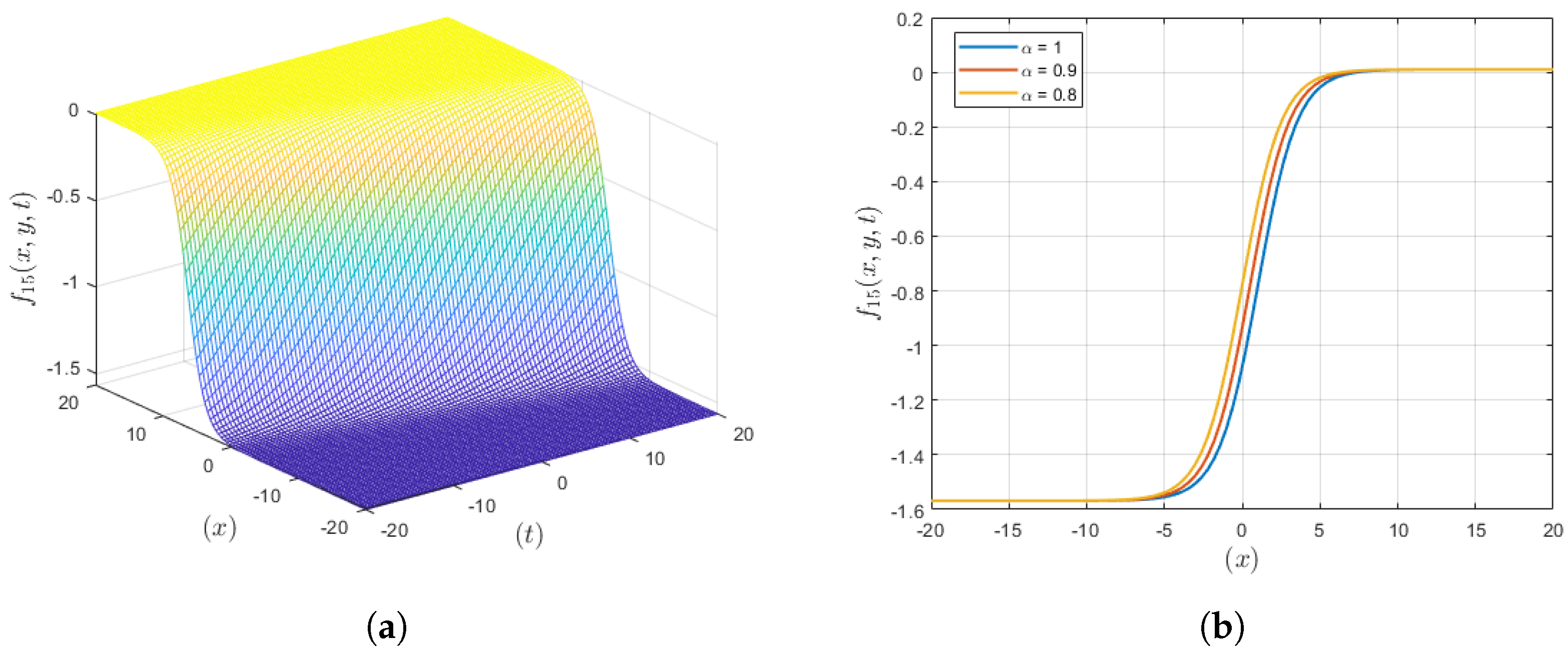
4. Results and Discussion

Further in the given section, we explore the spatial visualization of the wave solutions derived from the fractional (DJKM) equation. The types of solutions which are identified are trigonometric, hyperbolic and rational solutions as observed from the $3D$ and $2D$ Figure 1, Figure 2, Figure 3, Figure 4, Figure 5 and Figure 6 for the parameter values $p=0.5$, $q=0.2$, $\lambda =0.01$, $\omega =0.1$, $Y_1=0.001$, $Y_2=0.01$, $y=0.2$ and $\gamma =0.1$.

Figure 1 shows the anti-kink wave solution. However, it can clearly be seen that as the fractional order is small, wave propagation characteristics change drastically. The amplitude of the solution is significantly huge in the medium in which the wave travels. The study shows how minor differences in the parameter of the fractional-order derivative cause different wave characteristics. This is important in the area such as fluid dynamics where innovative methods of propagating waves must be achieved. The solutions suggested show high amplitudes, which means that the interactions occurring in the medium are strong, and these characteristics may be required to explain certain actions or processes in different scientific disciplines.

The compacton kink wave solution of the solution ($f_4$) is portrayed in Figure 2, which presents the effects of the used fractional order of the derivatives. Hence, the analysis of the $2D$ plot reveals that the amplitude of the wave is highly affected by the use of the fractional-order parameter that implies great changes in wave behavior. The illustration for integer-order derivatives in $3D$ has a localized high amplitude wavelet form and keeps within a finite area of space while oscillating. These plots suggest that fractional derivatives result in significantly higher and higher amplitude oscillations in contrast to integer-order derivatives, which is quite important in fluid dynamics, chemical kinetics and biological morphogenesis applications.

The graphical representation of the anti-kink wave solution ($f_6$) is depicted in Figure 3, where it is revealed that compared to the integer order, the fractional order gives a more localized waveform. If the virtue involves fractional derivatives, then the $2D$ plot reflects more confined waves, while in case of integer-order derivatives, the $3D$ plot illustrates less confined structures. This improved localization is useful for applications that demand a specific manipulation of the wave as in the case of drug delivery or optic fiber communications, hence increasing the probability of the accomplishment of the intended goal through the management of waves.

Figure 4 illustrates how any changes to the parameter ($\alpha$), which is dependent on a fractional order, are concentrated at anti-kink waves as opposed to when the parameter ($\alpha$) depends on an integer order. Plot $2D$ demonstrates that fractional derivatives give a more bound and narrow wavefront, and the third plot for integer-order derivatives reveals a broader wave front. This behavior can be rationalized in terms of long water waves where problems of frequency dispersion and nonlinear restoring forces are recognized as weak. Whereas localizations improve the description of the wave propagation, describing long water waves under these circumstances, fractional derivatives are of extreme value. The use of fractional derivatives is important when it comes to tuning the position of waves in order to model and predict the behavior of waves in situations where both dispersion as well as weak nonlinearity are important.

The kink wave solution ($f_{13}$) is presented in Figure 5 to depict that the wave amplitude is higher in the fractional-order derivatives than in the integer-order derivatives. From the $2D$ plot, it can be observed that when increasing fractional-order parameters, the resulting wave amplitudes are much higher than the original wave amplitudes. The node $3D$ portrayal of the integer-order derivative looks like it possesses a lesser surge than the one depicted for the fractional-order solutions. This greater amplitude with fractional derivatives means a higher energy of wave propagation, which is beneficial in cases where more energy is to be transferred, such as that which is necessary in fluid dynamics and high-energy wave interactions involving models. The possibility of obtaining larger amplitudes in comparison with fractional-order derivatives gives a powerful tool for the improvement and management of waves in different scientific and engineering fields.

The anti-kink wave solution ($f_{15}$) is presented in Figure 6 where the amplitude of the wave is larger with fractional-order derivatives as compared to the integer order. As can be seen in the $2D$ plot, decreasing the fractional-order parameter results in much higher wave amplitudes. When regarding the $3D$ scenario, the integer-order derivative solution bears lower amplitudes compared with the corresponding fractional-order solution, which indicates much more outstanding and higher amplitudes of waveforms. Such behavior implies that while fractional-order derivatives magnify the intensity of the waves to which they are applied, they are more powerful and energetic. This characteristic is highly beneficial for instances where a greater energy of the waves is needed for the interaction with a substance or material such as in the flow dynamics of fluids. The idea of attaining bigger amplitudes with the help of fractional derivatives gives a flexible means for controlling the oscillatory response in a plethora of science and engineering fields.

5. Conclusions

In this study, we were able to obtain dynamical wave solutions of the time–space fractional (DJKM) equation using an exciting and very efficient method called Riccati–Bernoulli sub-ODE method through Bäcklund transformation. Indeed, the method used in the paper allowed us to construct different solitary wave solutions such as compacton kink, kink soliton, and anti-kink soliton solutions. From the analysis, it was shown that the fractional-order derivatives give better wave amplitude and localization compared with the integer-order derivatives. These discoveries are significant especially in cases such as application in fluid dynamics, chemical kinetics, and biological morphogenesis where the characteristics of the waves need to be controlled. With the enhanced higher amplitude and better localization, the fractional-order derivatives are useful in enhancing wave behavior in different scientific and engineering fields. In the future, nonlinear dependencies of the electro-osmotic flow through viscoelastic fluids will be investigated as well as comparing the obtained results with experimental data. In conclusion, the present paper shows that fractional-order derivatives play a critical role in wave solutions for providing ways to improve the characterization of dynamic waves in various systems.

References

1. Wang, M.L.; Zhou, Y.B.; Li, Z.B. Application of a homogeneous balance method to exact solutions of nonlinear equations in mathematical physics. Phys. Lett. A 1996, 216, 67–75. [Google Scholar] [CrossRef]
2. Fan, E.; Zhang, H. A note on the homogeneous balance method. Phys. Lett. A 1998, 246, 403–406. [Google Scholar] [CrossRef]
3. Mahak, N.; Akram, G. Exact solitary wave solutions of the (1+1)-dimensional Fokas-Lenells equation. Optik 2020, 208, 1–9. [Google Scholar] [CrossRef]
4. Rezazadeh, H.; Manafian, J.; Khodadad, F.S.; Nazari, F. Traveling wave solutions for density dependent conformable fractional diffusion-reaction equation by the first integral method and the improved tan (ϕ(x)/2)-expansion method. Opt. Quantum Electron. 2018, 50, 1–15. [Google Scholar] [CrossRef]
5. Lu, D. Jacobi elliptic function solutions for two variant Boussinesq equations. Chaos Soliton Fractals 2005, 24, 1373–1385. [Google Scholar] [CrossRef]
6. Jafari, H.; Kadkhoda, N.; Baleanu, D. Fractional Lie group method of the time-fractional Boussinesq equation. Nonlinear Dyn. 2015, 81, 1569–1574. [Google Scholar] [CrossRef]
7. Raza, N.; Aslam, M.R.; Rezazadeh, H. Analytical study of resonant optical solitons with variable coefficients in Kerr and non-Kerrlaw media. Opt. Quantum Electron. 2019, 51, 59. [Google Scholar] [CrossRef]
8. Gao, W.; Rezazadeh, H.; Pinar, Z.; Baskonus, H.M.; Sarwar, S.; Yel, G. Novel explicit solutions for the nonlinear Zoomeron equation by using newly extended direct algebraic technique. Opt. Quantum Electron. 2020, 52, 1–13. [Google Scholar] [CrossRef]
9. Abdel-Gawad, H.I.; Osman, M.S. On the Variational Approach for Analyzing the Stability of Solutions of Evolution Equations. Kyungpook Math. J. 2013, 53, 661–680. [Google Scholar] [CrossRef]
10. Abdel-Gawad, H.I.; Osman, M. On shallow water waves in a medium with time-dependent dispersion and nonlinearity coefficients. J. Adv. Res. 2014, 6, 593–599. [Google Scholar] [CrossRef]
11. Ali, M.N.; Osman, M.S.; Husnine, S.M. On the analytical solutions of conformable time-fractional extended Zakharov-Kuznetsov equation through (G/G2)-expansion method and the modified Kudryashov method. SeMA J. 2019, 76, 15–25. [Google Scholar] [CrossRef]
12. Ali, K.K.; Osman, M.; Abdel-Aty, M. New optical solitary wave solutions of Fokas-Lenells equation in optical fiber via Sine-Gordon expansion method. Alex. Eng. J. 2020, 59, 1191–1196. [Google Scholar] [CrossRef]
13. Kumar, A.; Pankaj, R.D. Tanh–coth scheme for traveling wave solutions for Nonlinear Wave Interaction model. J. Egypt. Math. Soc. 2015, 23, 282–285. [Google Scholar] [CrossRef]
14. Domairry, G.; Mohsenzadeh, A.; Famouri, M. The application of homotopy analysis method to solve nonlinear differential equation governing Jeffery–Hamel flow. Commun. Nonlinear Sci. Numer. Simul. 2009, 14, 85–95. [Google Scholar] [CrossRef]
15. Zhang, Z.Y. Exact traveling wave solutions of the perturbed Klein-Gordon equation with quadratic nonlinearity in (1+1)-dimension. Part I: Without local inductance and dissipation effect. Turk. J. Phys. 2013, 37, 259–267. [Google Scholar] [CrossRef]
16. Fan, E. Extended tanh-function method and its applications to nonlinear equations. Phys. Lett. A 2000, 277, 212–218. [Google Scholar] [CrossRef]
17. Sarikaya, M.Z.; Budak, H.; Usta, H. On generalized the conformable fractional calculus. TWMS J. Appl. Eng. Math. 2019, 9, 792–799. [Google Scholar]
18. Akbar, M.A.; Ali, N.H.M.; Islam, M.T. Multiple closed form solutions to some fractional order nonlinear evolution equations in physics and plasma physics. AIMS Math. 2019, 4, 397–411. [Google Scholar] [CrossRef]
19. Liu, T. Exact solutions to time-fractional fifth order KdV equation by trial equation method based on symmetry. Symmetry 2019, 11, 742. [Google Scholar] [CrossRef]
20. Alshammari, S.; Al-Sawalha, M.M.; Shah, R. Approximate analytical methods for a fractional-order nonlinear system of Jaulent–Miodek equation with energy-dependent Schrodinger potential. Fractal Fract. 2023, 7, 140. [Google Scholar] [CrossRef]
21. Alderremy, A.A.; Shah, R.; Iqbal, N.; Aly, S.; Nonlaopon, K. Fractional series solution construction for nonlinear fractional reaction-diffusion Brusselator model utilizing Laplace residual power series. Symmetry 2022, 14, 1944. [Google Scholar] [CrossRef]
22. Yasmin, H.; Alshehry, A.S.; Ganie, A.H.; Mahnashi, A.M. Perturbed Gerdjikov–Ivanov equation: Soliton solutions via Backlund transformation. Optik 2024, 298, 171576. [Google Scholar] [CrossRef]
23. Elsayed, E.M.; Nonlaopon, K. The Analysis of the Fractional-Order Navier-Stokes Equations by a Novel Approach. J. Funct. Spaces 2022, 2022, 8979447. [Google Scholar] [CrossRef]
24. Alqhtani, M.; Saad, K.M.; Weera, W.; Hamanah, W.M. Analysis of the fractional-order local Poisson equation in fractal porous media. Symmetry 2022, 14, 1323. [Google Scholar] [CrossRef]
25. Hajar, F.I.; Hasan, B.; Choonkil, P.; Osman, M.S. M-lump, N-soliton solutions, and the collision phenomena for the (2+1)- dimensional Date–Jimbo–Kashiwara-Miwa equation. Results Phys. 2020, 19, 103329. [Google Scholar]
26. Wazwaz, A.M. A (2+1)–dimensional time–dependent Date–Jimbo–Kashiwara–Miwa equation: Painleve integrability and multiple soliton solutions. Comput. Math. Appl. 2020, 79, 1145–1149. [Google Scholar] [CrossRef]
27. Adem, A.R.; Yildirim, Y.; Yasar, E. Complexiton solutions and soliton solutions: (2+1)–dimensional Date–Jimbo–Kashiwara–Miwa equation. Pramana 2019, 92, 1–12. [Google Scholar] [CrossRef]
28. Yuan, Y.Q.; Tian, B.; Sun, W.R.; Chai, J.; Liu, L. Wronskian and Grammian solutions for a (2+1)-dimensional Date–Jimbo–Kashiwara–Miwa equation. Comp. Math. Appl. Int. J. 2017, 74, 873–879. [Google Scholar] [CrossRef]
29. Abdelrahman, M.A.E.; Sohaly, M.A. Solitary waves for the modified Korteweg-de Vries equation in deterministic case and random case. J. Phys. Math. 2017, 8, 214. [Google Scholar] [CrossRef]
30. Abdelrahman, M.A.E.; Sohaly, M.A. Solitary waves for the nonlinear Schrödinger problem with the probability distribution function in the stochastic input case. Eur. Phys. J. Plus 2017, 132, 339. [Google Scholar] [CrossRef]
31. Yang, X.F.; Deng, Z.C.; Wei, Y. A Riccati-Bernoulli sub-ODE method for nonlinear partial differential equations and its application. Adv. Differ. Equ. 2015, 1, 117–133. [Google Scholar] [CrossRef]
32. Lu, D.; Shi, Q. New Jacobi elliptic functions solutions for the combined KdV-mKdV equation. Int. J. Nonlinear Sci. 2010, 10, 320–325. [Google Scholar]
33. Zhang, Y. Solving STO and KD equations with modified Riemann-Liouville derivative using improved (G/G)-expansion function method. Int. J. Appl. Math. 2015, 45, 16–22. [Google Scholar]
Figure 1. Analyzing the influence of the derivative parameter ( α ) for both the fractional and integer order of the solution ( f 1 ) . (a) Three-dimensional (3D) depiction for the solution ( f 1 ) for integer-order derivative parameter ( α ). (b) Two-dimensional (2D) depiction for the solution ( f 1 ) for fractional-order derivative parameter ( α ).
Fractalfract 08 00497 g001
Figure 2. Analyzing the influence of the derivative parameter ( α ) for both the fractional and integer order of the solution ( f 4 ) . (a) Three-dimensional (3D) depiction for the solution ( f 4 ) for integer-order derivative parameter ( α ). (b) Two-dimensional (2D) depiction for the solution ( f 4 ) for fractional-order derivative parameter ( α ).
Fractalfract 08 00497 g002
Figure 3. Analyzing the influence of the derivative parameter ( α ) for both the fractional and integer order of the solution ( f 6 ) . (a) Three-dimensional (3D) depiction for the solution ( f 6 ) for integer-order derivative parameter ( α ). (b) Two-dimensional (2D) depiction for the solution ( f 6 ) for fractional-order derivative parameter ( α ).
Fractalfract 08 00497 g003
Figure 4. Analyzing the influence of the derivative parameter ( α ) for both the fractional and integer order of the solution ( f 9 ) . (a) Three-dimensional (3D) depiction for the solution ( f 9 ) for integer-order derivative parameter ( α ). (b) Two-dimensional (2D) depiction for the solution ( f 9 ) for fractional-order derivative parameter ( α ).
Fractalfract 08 00497 g004
Figure 5. Analyzing the influence of the derivative parameter ( α ) for both the fractional and integer order of the solution ( f 13 ) . (a) Three-dimensional (3D) depiction for the solution ( f 13 ) for integer-order derivative parameter ( α ). (b) Two-dimensional (2D) depiction for the solution ( f 13 ) for fractional-order derivative parameter ( α ).
Fractalfract 08 00497 g005
Figure 6. Analyzing the influence of the derivative parameter ( α ) for both the fractional and integer order of the solution ( f 15 ) . (a) Three-dimensional (3D) depiction for the solution ( f 15 ) for integer-order derivative parameter ( α ). (b) Two-dimensional (2D) depiction for the solution ( f 15 ) for fractional-order derivative parameter ( α ).
Fractalfract 08 00497 g006
Disclaimer/Publisher’s Note: The statements, opinions and data contained in all publications are solely those of the individual author(s) and contributor(s) and not of MDPI and/or the editor(s). MDPI and/or the editor(s) disclaim responsibility for any injury to people or property resulting from any ideas, methods, instructions or products referred to in the content.