Abstract
This study presents the application of the model expansion technique to find exact solutions for the (3+1)-dimensional space-time fractional modified KdV-Zakharov-Kuznetsov equation under Jumarie’s modified Riemann–Liouville derivative (JMRLD). The suggested method captures dark, periodic, traveling, and singular soliton solutions, providing deep insights into wave behavior. Clear graphics demonstrate that the solutions are greatly affected by changes in the fractional order, deepening our understanding and revealing the hidden dynamics of wave propagation. The considered equation has several applications in fluid dynamics, plasma physics, and nonlinear optics.
1. Introduction
Differential equations play important role in the modelling of physical phenomena [1,2]. Besides this, fractional differential equations (FDEs) have gained important attention in recent years due to their growing application in modeling complex nonlinear phenomena across several fields of science, containing physics, biology, mathematics, economics, engineering, and others [3,4]. These equations are used to define real-world systems, which are then explained into mathematical models. As a result, the quest of exact solutions for FDEs is essential in scientific research [5,6,7].
FDEs are an expansion of classical differential equations. Differentiation orders may be any real number, instead of just integers as in traditional differential equations. This makes FDEs much better at modeling complex system dynamics, especially in cases that show non-locality or memory features [8]. Applications for FDEs are numerous and varied starting from modelling population dynamics and chemical reactions, all the way to involving behavioral phenomena of materials and systems in physics and engineering [9,10,11].
In the investigation of FDEs, new analytical and numerical methods are developed for solving these equations, with prevailing among them the Adomian decomposition method [12], homotopy perturbation method [13], variational iteration method [14], and matrix approach method [15], between others. The method selected usually depends on the specific problem at hand and the required level of accuracy.
Fractional soliton solutions, arising from FDEs, have diverse applications across scientific and engineering fields. They model phenomena in nonlinear optical fibers, plasma physics, and fluid dynamics, where standard solitons fall short due to non-local effects. In quantum mechanics, they describe wave functions with unique dispersion properties, while in biological systems, they capture wave propagation with memory effects. Their applications extend to financial modeling, acoustics, epidemiology, control systems, and material science, offering insights into complex behaviors and interactions in these areas [16,17,18,19].
Recently, nonlinear integrable systems and their soliton solutions have attracted the attention of the researchers. Various soliton solutions of integrable systems have been investigated in the literature. For instance, Chen–Lee–Liu equation [20], Sasa-Satsuma equation [21], Drinfel’d–Sokolov–Wilson equation [22], pKP-BKP integrable equation [23], complex Ginzburg–Landau equation [24], Chaffee–Infante equation [25], nonlinear Zakharov system [26], and many more [27,28]. The (3+1)-dimensional modified Korteweg-de Vries-Zakharov-Kuznetsov ((3+1)-D MKDV-ZK) equation is a mathematical equation that shows the propagation of nonlinear waves in four-dimensional space time. It’s an extension of the classic KdV equation, which expresses solitary wave phenomena, and the Zakharov-Kuznetsov equation, which explanations for wave propagation in plasmas. The revised equation contains additional terms or modifications for a better explanation of actual phenomena. It’s commonly used to examine various physical systems such as fluid dynamics and nonlinear optics where it gives an understanding of complex wave behaviors [29,30]. The following expression has been proposed to offer a generalized version of the classical KdV equation to have fractional derivatives taken as per the modified Riemann-Liouville derivative.
(3+1)-D MKDV-ZK.
Here is an arbitrary constant.
Various techniques have been developed to solve the (3+1)-D MKDV-ZK equation, containing the method of undetermined coefficients [31], the ansatz method [32], the functional variable method [33], and the exp-function method [34]. These methods were applied for getting different types of solutions like solitons, dark solitons etc. In addition to this, they have also been working on studying a number of different cases including (3+1)-D MKDV-ZK equation in different fields of physics related to other aspects of nonlinear waves, solitons, etc. The equation is also related to fractional calculus and its applications in modeling complex systems.
The method that we have suggested provides exact solutions to complicated equations such as the (3+1)-D MKDV-ZK equation. Taking into account JMRLD and model expansion method of Jumarie makes it a fairly extensive observation of wide soliton behaviors. The power of the proposed approach lies in its ability to solve fractional derivative nonlinear wave equations properly and effectively in order to capture different wave phenomena. This method has wide applications such as in fluid dynamics and nonlinear optics where exact control of nonlinear wave dynamics is useful in forecasting actual systems.
The unique thing about this research is how it addresses the research gap by modeling complex wave dynamics exactly. Previous attempts often needed accuracy and completeness to achieve broad soliton behaviors depending on numerical approximations or simplification techniques. This study contributes by providing exact solutions to the (3+1)-D MKDV-ZK equations, thereby filling the research gap. Thus, this investigation significantly improves our capability for modeling and understanding nonlinear wave phenomena through a new approach for obtaining exact solutions which are different from those used before.
This paper proposes employing JMRLD [35] in combination with model expansion method to obtain exact solutions for nonlinear FPDEs. The primary objective of this study is to demonstrate the efficiency of this approach by utilizing it to derive exact solutions for FPDEs in both spatial and temporal domains related to JMRLD. The study will propose future possibilities, like extending the method to new equations, refining techniques for complexity, and exploring practical applications. It will highlight how these efforts can advance scientific understanding and solve real-world problems effectively.
The JMRLD of order is defined by the following expression [36]:
Here describes a function that is continuous.
Property 1.
Suppose that describes a function that is continuous from . We will use the considered equality for the integral via :
Property 2.
Property 3.
Property 4.
Property 5.
where c is constant.
2. Methodology
Here in the section, we provide briefly discuss the model expansion technique. Let us take a nonlinear partial differential equation(PDE).
where, is a polynomial with is a unknown partial derivatives.
The scheme contains following steps:
Step 1:
Taking the traveling wave transformation defined as:
The transformation given above will turn Equation (8) into ordinary differential equation (ODE). where and s are arbitrary constants.
where N is a polynomial of transformed ordinary derivatives , , , , …
Step 2:
Let the formal solution of Equation (10) is:
are constants for and follows the below auxiliary non-linear ODE.
here, is a real constant for .
Step 4:
Obtaining solution for Equation (8):
here and satisfy the Jacobian Elliptic equation (JEE):
where are constants for .
The values of m and n are defined as:
under the constraint condition:
Step 5:
The JEE for Equation (14), are given in the table below.
| Sr. No. | ||||
| 1 | 1 | or | ||
| 2 | ||||
| 3 | −1 | |||
| 4 | 1 | or | ||
| 5 | ||||
| 6 | −1 | |||
| 7 | 1 | |||
| 8 | 1 | |||
| 9 | 1 | |||
| 10 | 1 | |||
| 11 | or | |||
| 12 | ||||
| 13 | ||||
| 14 |
To obtain analytic solutions to the equation, jacobian elliptic functions (JEF) limitations are given in the table.
| function | function | ||||
| 1 | 1 | ||||
| 1 | 1 | ||||
3. Implementation of the Expansion Method
Through balancing the term , we get . After substituting the value obtained for s, we get formal solution expansion as:
where are constants, and . For getting algebraic equations we make use of Equation (18), Equation (13), and Equation (10), by setting them equal to zero, we obtain.
We use Mathematica 13.0 for computing these constants from the above-mentioned algebraic equations.
The obtained analytic answers of Equation (1) are:
Case 1:
If then = or , we obtain the JEF solutions as:
where and are given below as
subject to condition obtained as:
when
As then we obtained:
or then we get:
Subject to condition computed as:
When
As then we obtain:
or then we get:
Under the condition interpreted as:
Case 2:
If , then = the JEF solution is as:
where m and n are of the form:
Under the condition which interpret as:
When
As then we obtained
subject to condition which computes as:
Now when
As then we obtained:
subject to condition which is interpreted as:
Case 3:
If , then = we obtain the JEF solution as:
where and are as:
Under condition:
If
As then we get:
subject to interpreted constraint:
Now when
As then we obtained:
subject to a condition which is interpreted as:
Case 4:
If , then = or the JEF solution can given as:
here and are as:
Subject to interpreted condition:
if
As then we get:
Or so we get:
subject to a condition which is interpreted as:
Now when
As so we obtain:
Or so
under constraint condition:
Case 5:
If , then = obtained the JEF solutions as:
here and are:
Subject to interpreted condition:
if
As we get:
With the following constraint:
When
As then we get:
under computed constraint condition:
Case 6:
If , then = the JEF solution is as:
where and are:
Under condition:
when
As then we obtained:
Under condition interpreted as:
If
As then we get:
under interpret constraint:
Case 7:
If , then = JEF solution as:
here and are:
Under the interpreted condition:
when
As then we get:
subject to computed constraint:
Now if
As then,
under condition:
Case 8:
If , then = obtained JEF solution is as:
where and are:
under condition interpreted as:
now if
As then:
subject to the computed condition:
If
As then
under interpreted constraint condition:
Case 9:
If , then = the JEF solution is as:
here and are as:
Subject to the condition:
Now If
As then we get:
under the constraint condition:
If
As then we got:
subject to interpreted condition:
Case 10:
If , then = we obtained the JEF solution as:
where and are,
Under condition:
If
As then we get:
under the interpreted constraint condition:
Now if
As we get:
under computed constraint condition:
Case 11:
If , then = then JEF solution obtained as:
here and are as:
Subject to interpreted condition:
Now if
As then we get:
also,
condition which computes as:
Now if
As then we get:
or then we get:
under condition which interpreted as:
Case 12:
If , then = then JEF solution is as:
here and are,
Under condition:
now if
As then we get:
subject to interpreted condition:
now if
As then:
under computed condition:
Case 13:
If , then = then JEF solution is as:
here and are,
Under interpreted condition:
now if
As then
under interpreted constraint condition:
Now if
As then
subject to interpreted condition:
Case 14:
If , then = then JEF solution is as:
here and are as:
Subject to an interpreted condition:
Now if
As then:
under condition:
If
As then
under defined constraint condition:
4. Graphical Illustration and Discussion
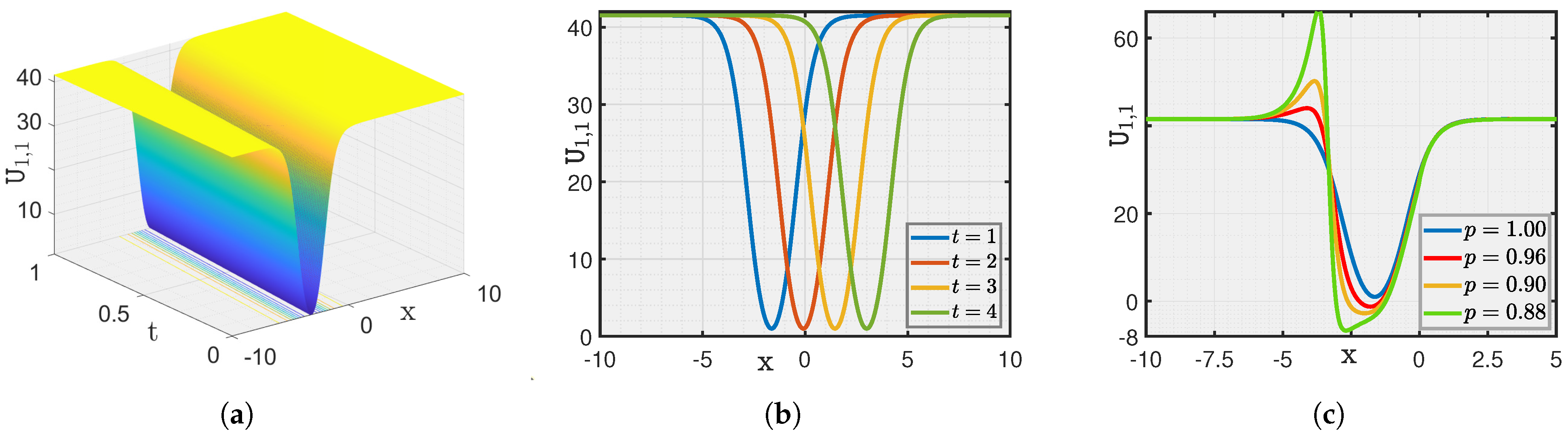
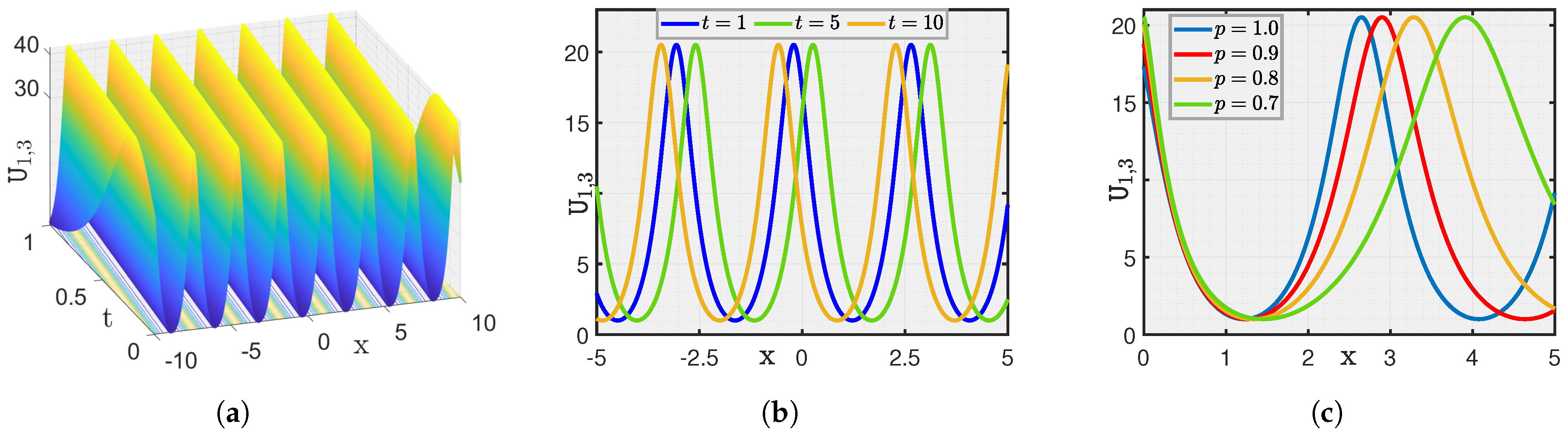
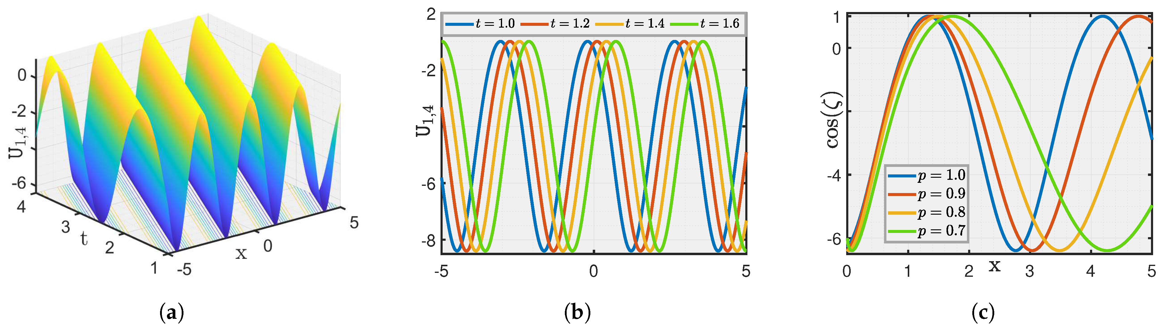
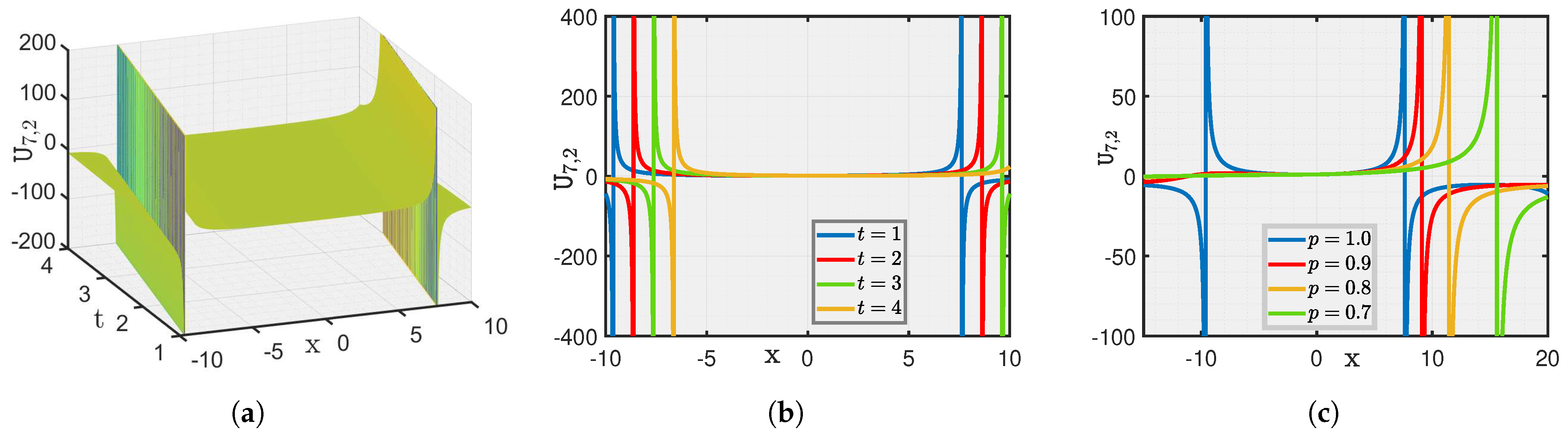
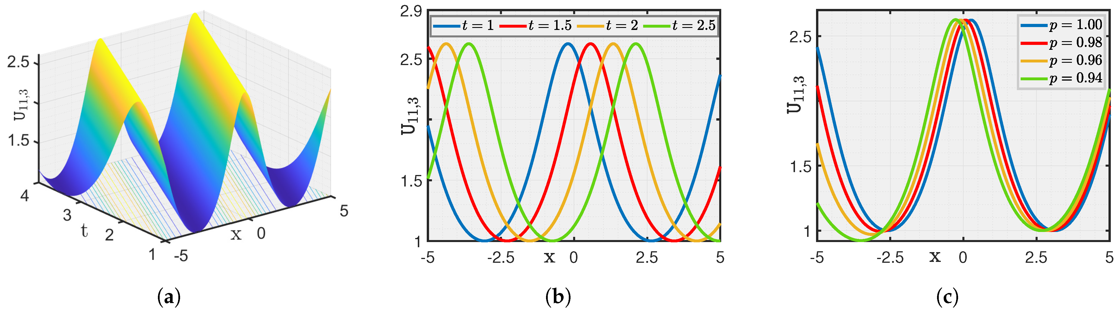
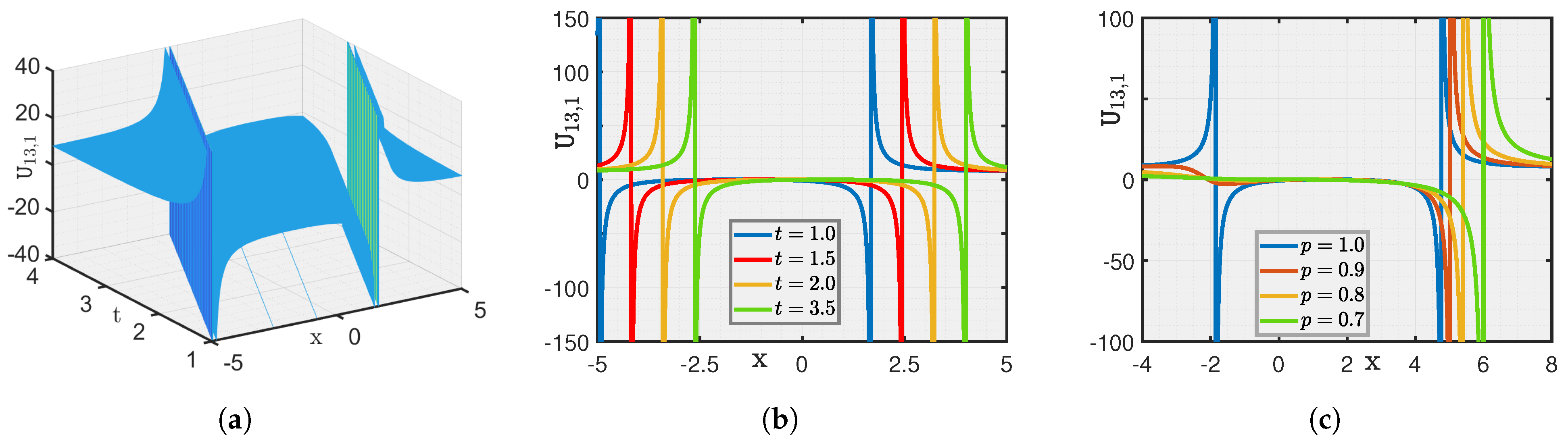
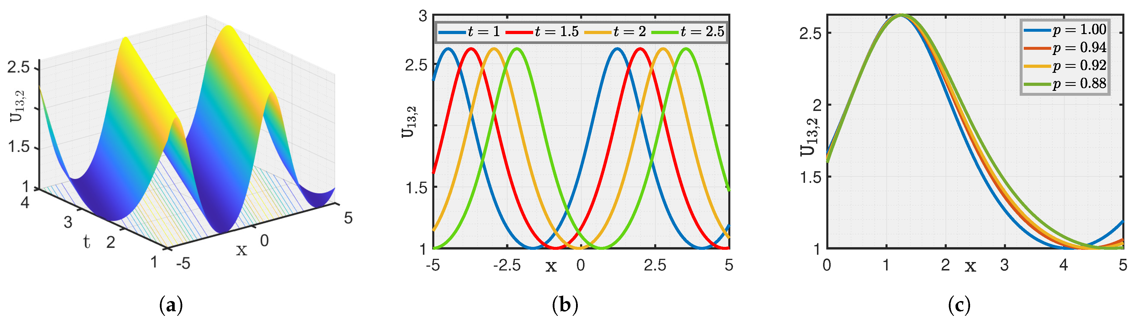
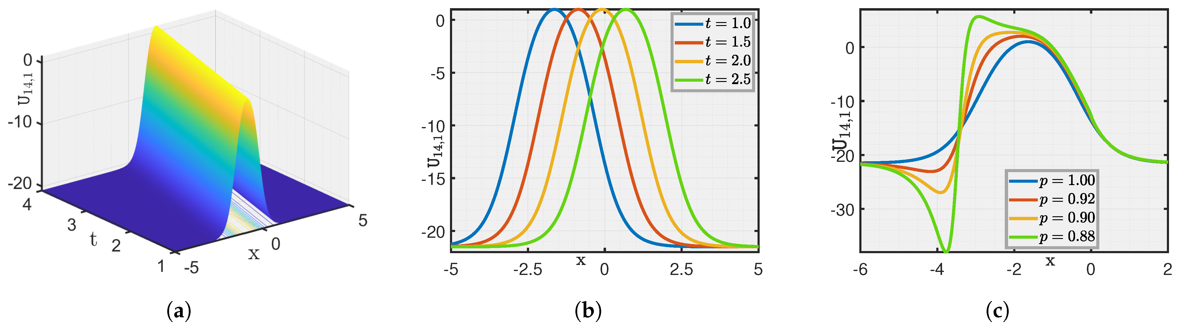
Here, we show a graphical illustration of some of the obtained new analytical soliton solutions for the (3+1)-dimensional fractional (mKDV-ZK) equation, including periodic soliton, bright soliton dark soliton, and singular periodic soliton. They are visualized in Figure 1, Figure 2, Figure 3, Figure 4, Figure 5, Figure 6, Figure 7 and Figure 8 via 3D and 2D for different values of t. We also show the effect of fractional parameters on the obtained solutions through 2D for different fractional order shown in each legend of the graph. In Figure 1, we plot the solution represented by , which shows the dark soliton behaviour. Moreover, we show periodic solitons through Figure 2, Figure 3, Figure 4, Figure 5, Figure 6 and Figure 7 representing by respectively. Additionally, we also plot singular solitons through Figure 4 and Figure 6 representing by . Lastly, we show Bright Soliton solution represented by through Figure 8. The innovation of these solutions can be observed as that they provide new analytical expressions for soliton solutions of the fractional mKdV-ZK equation, which has not been widely studied in the literature. These solutions will be more helpful in the understanding of nonlinear wave dynamics narrated by the considered equation, which is applicable in many physical systems such as fluid dynamics, plasma physics, and nonlinear optics. The gained soliton solutions can be applied to model and examine the propagation of periodic wave patterns, localized wave packets, and singular wave profiles in systems reign over by the fractional mKdV-ZK equation, together with applications in plasma turbulence, shallow water waves, and optical communications.
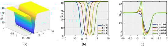
Figure 1.
(a–c) Visualization of for .
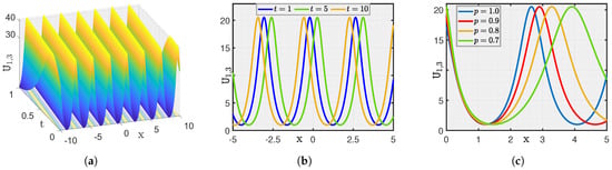
Figure 2.
(a–c) Visualization of for .
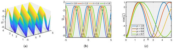
Figure 3.
(a–c) Visualization of for .
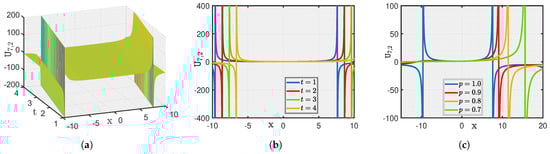
Figure 4.
(a–c) Visualization of for .

Figure 5.
(a–c) Visualization of for .

Figure 6.
(a–c) Visualization of for .
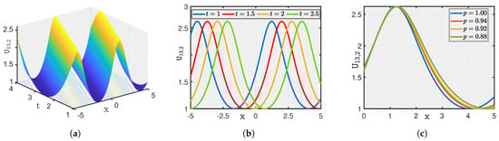
Figure 7.
(a–c) Visualization of for .
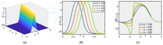
Figure 8.
(a–c) Visualization of for .
5. Conclusions
This study has well focused on the challenge of solving the (3+1)-dimensional space-time fractional modified KdV-ZK equation by using the model expansion method with Jumarie’s modified RL derivative. The method has been confirmed effective in arising exact solutions that widely capture some soliton behaviors, containing dark, periodic, traveling, and singular solitons. The effect of the fractional order on the propagation of waves has been clearly presented via graphs. The dynamics of the soliton solutions were different when we varied the fractional order. These results significantly contribute to proceeding with our understanding of nonlinear wave dynamics and have wide implications across scientific disciplines, including fluid dynamics, plasma physics, and nonlinear optics. The exact solutions obtained surpass previous efforts and present a strong framework for exactly modeling complex wave phenomena. Moving forward, further research could explore extending the method to other equations, refining techniques for handling complexity, and exploring practical applications in specific fields.
Author Contributions
Conceptualization, O.O.; methodology, M.U.S.; formal analysis, M.H.; investigation, M.H.; writing—original draft preparation, K.A.; writing—review and editing, A.E.H. and H.S.; software, O.O. and M.U.S. All authors have read and agreed to the published version of the manuscript.
Funding
This research received no external funding.
Data Availability Statement
No new data were created or analyzed in this study. Data sharing is not applicable to this article.
Acknowledgments
The Researchers would like to thank the Deanship of Graduate Studies and Scientific Research at Qassim University for financial support (QU-APC-2024-9/1). Khaled Aldwoah wishes to extend his sincere gratitude to the Deanship of Scientific Research at the Islamic University of Madinah.
Conflicts of Interest
The authors declare no conflict of interest.
References
- Li, C.; Zhu, C.X.; Zhang, N.; Sui, S.H.; Zhao, J.B. Free vibration of self-powered nanoribbons subjected to thermal-mechanical-electrical fields based on a nonlocal strain gradient theory. Appl. Math. Model. 2022, 110, 583–602. [Google Scholar] [CrossRef]
- Zhu, C.; Chen, Y.; Zhao, J.; Li, C.; Lei, Z. On Nonlocal Vertical and Horizontal Bending of a Micro-Beam. Math. Probl. Eng. 2022, 2022, 5121377. [Google Scholar] [CrossRef]
- Xu, C.; Farman, M.; Shehzad, A. Analysis and chaotic behavior of a fish farming model with singular and non-singular kernel. Int. J. Biomath. 2023. [Google Scholar] [CrossRef]
- Xu, C.; Liao, M.; Farman, M.; Shehzad, A. Hydrogenolysis of glycerol by heterogeneous ca-talysis: A fractional order kinetic model with analysis. MATCH Commun. Math. Comput. Chem. 2024, 91, 635–664. [Google Scholar] [CrossRef]
- Miller, K.S.; Ross, B. An Introduction to the Fractional Calculus and Fractional Differential Equations; Wiley: Hoboken, NJ, USA, 1993. [Google Scholar]
- Sutradhar, T.; Datta, B.K.; Bera, R.K. Analytical solution of the time fractional Fokker-Planck equation. Int. J. Appl. Mech. Eng. 2014, 19, 435–440. [Google Scholar] [CrossRef]
- Khan, A.; Akram, T.; Khan, A.; Ahmad, S.; Nonlaopon, K. Investigation of time fractional nonlinear KdV-Burgers equation under fractional operators with nonsingular kernels. AIMS Math 2023, 8, 1251–1268. [Google Scholar] [CrossRef]
- Guo, L.; Li, C.; Zhao, J. Existence of Monotone Positive Solutions for Caputo–Hadamard Nonlinear Fractional Differential Equation with Infinite-Point Boundary Value Conditions. Symmetry 2023, 15, 970. [Google Scholar] [CrossRef]
- Nieto, J.J.; Khastan, A.; Ivaz, K. Numerical solution of fuzzy differential equations under generalized differentiability. Nonlinear Anal. Hybrid Syst. 2009, 3, 700–707. [Google Scholar] [CrossRef]
- Collegari, R.; Federson, M.; Frasson, M. Linear FDEs in the frame of general-ized ODEs: Variation-of-constants formula. Czechoslov. Math. J. 2018, 68, 889–920. [Google Scholar] [CrossRef]
- Khan, A.; Ali, A.; Ahmad, S.; Saifullah, S.; Nonlaopon, K.; Akgül, A. Nonlinear Schrö-dinger equation under non-singular fractional operators: A computational study. Results Phys. 2022, 43, 106062. [Google Scholar] [CrossRef]
- Duan, J.S.; Rach, R.; Baleanu, D.; Wazwaz, A.M. A review of the Adomian de-composition method and its applications to fractional differential equations. Commun. Fract. Calc. 2012, 3, 73–99. [Google Scholar]
- He, J.-H. Recent development of the homotopy perturbation method. Topol. Methods Nonlinear Anal. 2008, 31, 205–209. [Google Scholar]
- Abdou, M.A.; Soliman, A.A. New applications of variational iteration method. Phys. D Nonlinear Phenom. 2005, 211, 1–8. [Google Scholar] [CrossRef]
- Podlubny, I.; Chechkin, A.; Skovranek, T.; Chen, Y.; Jara, B.M. Matrix approach to discrete fractional calculus II: Partial fractional differential equations. J. Comput. Phys. 2009, 228, 3137–3153. [Google Scholar] [CrossRef]
- Iqbal, M.A.; Miah, M.M.; Ali, H.S.; Shahen, N.H.M.; Deifalla, A. New applications of the fractional derivative to extract abundant soliton solutions of the fractional order PDEs in mathematics physics. Partial. Differ. Equ. Appl. Math. 2024, 9, 100597. [Google Scholar] [CrossRef]
- Younas, U.; Yao, F.; Nasreen, N.; Khan, A.; Abdeljawad, T. On the dynamics of soliton solutions for the nonlinear fractional dynamical system: Application in ultrasound imaging. Results Phys. 2024, 57, 107349. [Google Scholar] [CrossRef]
- Yasin, S.; Khan, A.; Ahmad, S.; Osman, M.S. New exact solutions of (3+1)-dimensional modified KdV-Zakharov-Kuznetsov equation by Sardar-subequation method. Opt. Quantum Electron. 2024, 56, 90. [Google Scholar] [CrossRef]
- Khan, A.; Khan, A.U.; Ahmad, S. Investigation of fractal fractional nonlinear Korteweg-de-Vries-Schrödinger system with power law kernel. Phys. Scr. 2023, 98, 085202. [Google Scholar] [CrossRef]
- Baber, M.Z.; Ahmed, N.; Xu, C.; Iqbal, M.S.; Sulaiman, T.A. A computational scheme and its comparison with optical soliton solutions for the stochastic Chen–Lee–Liu equation with sensitivity analysis. Mod. Phys. Lett. B 2024, 2450376. [Google Scholar] [CrossRef]
- Li, P.; Shi, S.; Xu, C.; ur Rahman, M. Bifurcations, chaotic behavior, sensitivity analysis and new optical solitons solutions of Sasa-Satsuma equation. Nonlinear Dyn. 2024, 112, 7405–7415. [Google Scholar] [CrossRef]
- Akram, W.; Ullah, A.; Ali, S.; Ahmad, S. Exploration of soliton solution of coupled Drinfel’d–Sokolov–Wilson equation under conformable differential operator. Partial. Differ. Equ. Appl. Math. 2024, 10, 100708. [Google Scholar] [CrossRef]
- Saifullah, S.; Ahmad, S.; Khan, M.A.; ur Rahman, M. Multiple solitons with fission and multi waves interaction solutions of a (3+1)-dimensional combined pKP-BKP integrable equation. Phys. Scr. 2024, 99, 065242. [Google Scholar] [CrossRef]
- Zhu, C.; Al-Dossari, M.; Rezapour, S.; Alsallami, S.A.M.; Gunay, B. Bifurcations, chaotic be-havior, and optical solutions for the complex Ginzburg–Landau equation. Results Phys. 2024, 59, 107601. [Google Scholar] [CrossRef]
- Zhu, C.; Al-Dossari, M.; Rezapour, S.; Gunay, B. On the exact soliton solutions and different wave structures to the (2+1) dimensional Chaffee–Infante equation. Results Phys. 2024, 57, 107431. [Google Scholar] [CrossRef]
- Zhu, C.; Al-Dossari, M.; Rezapour, S.; Shateyi, S.; Gunay, B. Analytical optical solutions to the nonlinear Zakharov system via logarithmic transformation. Results Phys. 2024, 56, 107298. [Google Scholar] [CrossRef]
- Kai, Y.; Ji, J.; Yin, Z. Study of the generalization of regularized long-wave equation. Nonlinear Dyn. 2022, 107, 2745–2752. [Google Scholar] [CrossRef]
- Kai, Y.; Yin, Z. Linear structure and soliton molecules of Sharma-Tasso-Olver-Burgers equation. Phys. Lett. A 2022, 452, 128430. [Google Scholar] [CrossRef]
- Sahoo, S.; Ray, S.S. Improved fractional sub-equation method for (3+1)-dimensional generalized fractional KdV–Zakharov–Kuznetsov equations. Comput. Math. Appl. 2015, 70, 158–166. [Google Scholar] [CrossRef]
- Guner, O. New exact solutions to the space–time fractional nonlinear wave equation obtained by the ansatz and functional variable methods. Opt. Quantum Electron. 2018, 50, 38. [Google Scholar] [CrossRef]
- Christiano, L.J. Solving dynamic equilibrium models by a method of unde-termined coefficients. Comput. Econ. 2002, 20, 21–55. [Google Scholar] [CrossRef]
- Park, C.; Nuruddeen, R.I.; Ali, K.K.; Muhammad, L.; Osman, M.S.; Baleanu, D. Novel hyperbolic and exponential ansatz methods to the fractional fifth-order Korteweg–de Vries equations. Adv. Differ. Equ. 2020, 2020, 627. [Google Scholar] [CrossRef]
- Liu, W.; Chen, K. The functional variable method for finding exact solutions of some nonlinear time-fractional differential equations. Pramana 2013, 81, 377–384. [Google Scholar] [CrossRef]
- Nisar, K.S.; Ilhan, O.A.; Abdulazeez, S.T.; Manafian, J.; Mohammed, S.A.; Osman, M.S. Novel multiple soliton solutions for some nonlinear PDEs via multiple Exp-function method. Results Phys. 2021, 21, 103769. [Google Scholar] [CrossRef]
- Jumarie, G. Modified Riemann–Liouville derivative and fractional Taylor series of nondifferentiable functions further results. Comput. Math. Appl. 2006, 51, 1367–1376. [Google Scholar] [CrossRef]
- Jumarie, G. Table of some basic fractional calculus formulae derived from a mod-ified Riemann–Liouvillie derivative for nondifferentiable functions. Appl. Math. Lett. 2009, 22, 378–385. [Google Scholar]
Disclaimer/Publisher’s Note: The statements, opinions and data contained in all publications are solely those of the individual author(s) and contributor(s) and not of MDPI and/or the editor(s). MDPI and/or the editor(s) disclaim responsibility for any injury to people or property resulting from any ideas, methods, instructions or products referred to in the content. |
© 2024 by the authors. Licensee MDPI, Basel, Switzerland. This article is an open access article distributed under the terms and conditions of the Creative Commons Attribution (CC BY) license (https://creativecommons.org/licenses/by/4.0/).