On the Numerical Investigations of a Fractional-Order Mathematical Model for Middle East Respiratory Syndrome Outbreak

Abstract

Middle East Respiratory Syndrome (MERS) is a human coronavirus subtype that poses a significant public health concern due to its ability to spread between individuals. This research aims to develop a fractional-order mathematical model to investigate the MERS pandemic and to subsequently develop two numerical methods to solve this model numerically to evaluate and comprehend the analysis results. The fixed-point theorem has been used to demonstrate the existence and uniqueness of the solution to the suggested model. We approximate the solutions of the proposed model using two numerical methods: the mean value theorem and the implicit trapezoidal method. The stability of these numerical methods is studied using various results and primary lemmas. Finally, we compare the results of our methods to demonstrate their efficiency and conduct a numerical simulation of the obtained results. A comparative study based on real data from Riyadh, Saudi Arabia is provided. The study’s conclusions demonstrate the computational efficiency of our approaches in studying nonlinear fractional differential equations that arise in daily life problems.

1. Introduction

The Middle East Respiratory Syndrome Coronavirus (MERS-CoV) is the virus that causes Middle East Respiratory Syndrome (MERS), a viral respiratory infection. First identified in Saudi Arabia in 2012, MERS is characterized by severe respiratory symptoms such as fever, coughing, and dyspnea. In extreme cases, these symptoms can progress to pneumonia and even respiratory failure. Close contact with infected people or their respiratory secretions is the main way that the virus spreads, while outbreaks have occasionally been documented in hospital environments. Despite having a relatively low transmission rate compared to other respiratory viruses like influenza1, MERS is considered a serious respiratory virus due to its high mortality rate, particularly among individuals with compromised immune systems or pre-existing medical conditions. MERS is one of the most dangerous viruses to emerge in recent years, with approximately thirty-five percent of those infected succumbing to the illness. MERS falls under the category of zoonotic viruses, meaning that an animal serves as both the virus’s carrier and its main source of transmission. The primary reservoir hosts and agents of MERS transmission are camels. This is because some camel caravans have antibodies against MERS [1,2].

The Arabian Peninsula boasts one of the world’s largest populations of camels. Consequently, it is no surprise that the Arabian Gulf region, encompassing Saudi Arabia, records the highest number of MERS cases. With almost 80% of cases, Saudi Arabia holds the highest infection rate in the Gulf. Moreover, camels are considered national resources in the Arabian Gulf region, where the populace frequently interacts with them. In this area, camel milk and meat are commonly consumed, and some people utilize camel urine in traditional healing methods, highlighting the close bond between camels and breeders along the Gulf Coast [1,3]. The infection seems geographically concentrated in the Middle East, with cases reported in Saudi Arabia, Qatar, Jordan, and the United Arab Emirates. However, it has spread to several other countries, including Algeria, Bangladesh, Indonesia, Kuwait, Egypt, Turkey, Oman, Italy, France, the United Kingdom, Germany, the United States, and South Korea [4]. Consequently, the illness has not only spread throughout the Gulf region but to 27 other countries globally.

Mathematical models of infectious diseases are extremely necessary to provide a detailed description of the spread of infectious diseases among populations [5]. These models are also useful resources for comprehending crucial elements of epidemics and the dynamics of newly developing infectious illnesses. On the other hand, to implement strategic plans to address and contain the threat of infectious diseases, decision-makers might utilize mathematical models to acquire knowledge about the behavior of epidemics and pandemics. A useful tool for characterizing epidemic dynamic systems is a fractional-order model [5,6,7]. These models, as opposed to traditional integer-order models, show a superior fit for real data that has been seen. The concept of memory, which exists in biological and epidemiological systems, is taken into consideration by fractional-order models [8,9]. It is possible to characterize memory that varies with time using the fractional variable-order derivatives, which are defined as an extension of the constant fractional-order derivatives [7,10,11].

The ongoing research into MERS aims to deepen our understanding of the virus’s transmission dynamics, pathogenesis, and potential treatment options. This includes the development of mathematical models to simulate and predict the spread of the virus, as well as efforts to develop vaccines and antiviral therapies. Understanding the factors influencing MERS transmission and severity is crucial for implementing effective public health measures to control outbreaks and minimize the impact of this potentially deadly disease [12,13,14,15,16,17,18,19,20,21].

2. Preliminaries

In this section, we present some fundamental concepts of fractional calculus as follows:

Definition 1.

Let $u\left(t\right)$ be a Lebesgue integrable function over the interval $\left[0, T\right]$. The Caputo derivative of fractional order $\alpha$ is described as follows [22]:

$$D_t^{\alpha }u\left(t\right)={\displaystyle \frac{1}{\mathrm{\Gamma }\left(n-\alpha \right)}}\underset{0}{\overset{t}{\int }}{\displaystyle \frac{d^{n}u\left(\tau \right)}{d{\tau }^n}}{\left(t-\tau \right)}^{n-\alpha -1}d\tau , n-1<\alpha <n, n\in \mathbb{N}.$$

(1)

Lemma 1.

Let $X\in C\left[0, T\right]$ be a solution of the Caputo fractional differential equation [23]:

$$D_t^{\alpha } X\left(t\right)=H\left(t, X\left(t\right)\right),X\left(0\right)=X_0, 0<\alpha <1,$$

(2)

if and only if it is a solution of the following nonlinear integral equation:

$$X\left(t\right)=X_0+{\displaystyle \frac{1}{\mathrm{\Gamma }\left(\mathsf{\alpha }\right)}}\underset{0}{\overset{t}{\int }}H\left(\tau ,X\left(\tau \right)\right){\left(t-\tau \right)}^{\mathsf{\alpha }-1}d\tau .$$

(3)

Lemma 2.

If $\alpha \in \left(0, 1\right)$ and the integer $j\ge 0$, then there exist the positive constants ${\mathfrak{K}}_{\alpha , 1}$ and ${\mathfrak{K}}_{\alpha , 2}$ dependent only on $\alpha$, such that [24]

$${\left(j+1\right)}^{\alpha }-j^{\alpha }\le {\mathfrak{K}}_{\alpha , 1}{\left(j+1\right)}^{\alpha -1},$$

(4)

and

$${\left(j+2\right)}^{\alpha +1}-2{\left(j+2\right)}^{\alpha +1}+j^{\alpha +1}\le {\mathfrak{K}}_{\alpha , 2}{\left(j+1\right)}^{\alpha -1}.$$

(5)

Lemma 3.

Consider that $c_{n, \mathrm{j}}={\left(j-n\right)}^{\alpha -1}$, $n=1, 2, \dots ,j-1$ and $c_{n, \mathrm{j}}=0$, for $n\ge j$, α, k, W, $M>0$, $tk\le M,$ and t is a positive integer. Let $\sum _{j=i}^n{c}_{n, \mathrm{j}}\left|a_n\right|=0$ for $i>n\ge 1$. If [24]

$$\left|a_n\right|\le W{k}^{\alpha }\sum _{n=1}^{n-1}{c}_{n, \mathrm{j}}\left|a_n\right|+\left|{\mu }_0\right|, n=1, 2, \dots , t,$$

(6)

then

$$\left|a_j\right|\le \theta \left|{\mu }_0\right|, n=1, 2, \dots$$

(7)

 where $\theta$ is a positive constant independent of k and t.

3. Model Derivation

This section establishes a fractional model of MERS, which is based on the model that is described in [4,25]. Five subpopulations are described: susceptible $S$, exposed or asymptomatic individuals $E$, infected individuals $I$, isolated individuals $J$, and recovered individuals $R$. These are time functions expressed in days. At time $t$, the total number of living individuals is represented by $N\left(t\right)=S\left(t\right)+E\left(t\right)+I\left(t\right)+J\left(t\right)+R\left(t\right)$. All living people who are not part of any other group are considered part of the susceptible population. The number of asymptomatic individuals who have been exposed to the virus but have not yet shown any clinical signs of MERS is indicated by the subpopulation E(t). The subpopulation $I\left(t\right)$ represents those who have MERS clinical symptoms. Individuals with isolated symptoms are represented by the subpopulation $J\left(t\right)$, while those who have recovered from MERS are represented by the subpopulation $R\left(t\right)$. The following system of ordinary differential equations presents the pandemic model for MERS [4]:

$$\begin{gathered} {\displaystyle \frac{dS\left(t\right)}{dt}}=P-{\displaystyle \frac{S\left(t\right)\left(\beta I\left(t\right)+{ϵ}_E\beta E\left(t\right)+{ϵ}_J\beta J\left(t\right)\right)}{N}}-\mu S\left(t\right), \\ {\displaystyle \frac{dE\left(t\right)}{dt}}={\displaystyle \frac{S\left(t\right)\left(\beta I\left(t\right)+{ϵ}_E\beta E\left(t\right)+{ϵ}_J\beta J\left(t\right)\right)}{N}}-\left({\rm K}+\mu \right)E\left(t\right), \\ {\displaystyle \frac{dI\left(t\right)}{dt}}={\rm K}E\left(t\right)-\left(\gamma +{\sigma }_1+d_1+\mu \right)I\left(t\right), \\ {\displaystyle \frac{dJ\left(t\right)}{dt}}=\gamma I\left(t\right)-\left({\sigma }_2+d_2+\mu \right)J\left(t\right), \\ {\displaystyle \frac{dR\left(t\right)}{dt}}={\sigma }_{1}I\left(t\right)+{\sigma }_{2}J\left(t\right)-\mu R\left(t\right). \end{gathered}$$

(8)

The initial conditions are

$$S\left(0\right)=S_0, E\left(0\right)=E_0, \mathrm{I}\left(0\right)=I_0, R\left(0\right)=R_0.$$

(9)

where the number of people who are born and enter the city every day is represented by $P$, while the population’s normal mortality rate is $\mu$ (1/day). $\beta$ (1/day) is the probability that one collision between an infected and a susceptible person will result in infection; correspondingly, ${ϵ}_E\beta$ (1/day) and ${ϵ}_J\beta$ (1/day) are the probabilities that one interaction between an isolated person and an infected person will result in infection, also $0\le {ϵ}_E, {ϵ}_J\le 1$ are the decrease factors in the spreading rates. The rate at which individuals develop clinical symptoms upon exposure is denoted by the parameter ${\rm K}$ (measured in 1/day). The isolation rate is represented by $\gamma$ (also measured in 1/day). Furthermore, in addition to the baseline mortality rate $\mu$, the disease-induced death rates among the infected and isolated populations are captured by the rate coefficients $d_1$ and $d_2$, respectively, with units of 1/day. Finally, ${\sigma }_1$ and ${\sigma }_2$ signify the rates of recovery for the infectious and isolated individuals, respectively.

Next, we replaced the time derivatives in Equations (8) and (9). with the Caputo fractional derivatives. The dimensions of the right and left sides differ because of this modification. To fix this issue, we modified the fractional operator such that the sides have the same dimension by using an auxiliary parameter $\chi$, which has the dimension of sec [26,27]. Then, Equations (8) and (9) become

$$\begin{gathered} {\chi }^{1-\alpha }{D}_t^{\alpha } S\left(t\right)=P-{\displaystyle \frac{S\left(t\right)\left(\beta I\left(t\right)+{ϵ}_{E }\beta E\left(t\right)+{ϵ}_{J }\beta J\left(t\right)\right)}{N}}-\mu S\left(t\right), \\ {\chi }^{1-\alpha }{D}_t^{\alpha } E\left(t\right)={\displaystyle \frac{S\left(t\right)\left(\beta I\left(t\right)+{ϵ}_{E }\beta E\left(t\right)+{ϵ}_{J }\beta J\left(t\right)\right)}{N}}-\left({\rm K}+\mu \right) E\left(t\right), \\ {\chi }^{1-\alpha }{D}_t^{\alpha } I\left(t\right)={\rm K} E\left(t\right)-\left(\gamma +{\sigma }_1+d_1+\mu \right) I\left(t\right), \\ {\chi }^{1-\alpha }{D}_t^{\alpha } J\left(t\right)=\gamma I\left(t\right)-\left({\sigma }_2+d_2+\mu \right) J\left(t\right), \\ {\chi }^{1-\alpha }{D}_t^{\alpha } R\left(t\right)={\sigma }_{1 }I\left(t\right)+{\sigma }_2 J\left(t\right)-\mu R\left(t\right), \end{gathered}$$

(10)

subject to the following initial conditions:

$$S\left(0\right)=S_0, E\left(0\right)=E_0, \mathrm{I}\left(0\right)=I_0, R\left(0\right)=R_0.$$

(11)

3.1. Stability and Equilibrium Points

Regarding system (10), we consider the equilibrium points [4].

$$D_t^{\alpha }S\left(t\right)=D_t^{\alpha }E\left(t\right)=D_t^{\alpha }I\left(t\right)=D_t^{\alpha }J\left(t\right)=D_t^{\alpha }R\left(t\right)=0.$$

(12)

We identified two equilibrium points as the disease-free equilibrium

$$E_0=\left({\displaystyle \frac{P}{\mu }},0, 0, 0, 0 \right)$$

and the endemic equilibrium

$$E_{*}=\left(S_{*},E_{*},I_{*},J_{*},R_{*}\right)=\left({\displaystyle \frac{P}{\mu +{\tau }_{*}}},{\displaystyle \frac{P{\tau }_{*}}{Q_1\left(\mu +{\tau }_{*}\right)}},{\displaystyle \frac{\mathrm{{\rm K}}{E}_{*}}{Q_2}},{\displaystyle \frac{\gamma \mathrm{{\rm K}}{E}_{*}}{Q_2{Q}_3}},{\displaystyle \frac{\mathrm{{\rm K}}{E}_{*}}{Q_2}}\left({\displaystyle \frac{{\sigma }_1}{\mu }}+{\displaystyle \frac{{\sigma }_2\gamma }{\mu Q_3}}\right)\right),$$

where

$Q_1=\mathrm{{\rm K}}+\mu$, $Q_2=\gamma +{\sigma }_1+d_1+\mu$, $Q_3={\sigma }_2+d_2+\mu$, $\sigma ={\displaystyle \frac{Q_3(\mu Q_2+{\rm K}({\sigma }_1+\mu \left)\right)+\gamma {\rm K}({\sigma }_2+\mu )}{Q_1{Q}_2{Q}_3}}$, and ${\tau }_{*}={\displaystyle \frac{\mu }{\sigma }}\left({\mathcal{R}}_c-1\right)$.

Also, the control reproduction number ${\mathcal{R}}_c={\displaystyle \frac{{\beta ϵ}_E}{Q_1}}+{\displaystyle \frac{\mathrm{{\rm K}}\beta }{Q_1{Q}_2}}+{\displaystyle \frac{\beta {ϵ}_{J}K\gamma }{Q_1{Q}_2{Q}_3}}$.

Theorem 1.

The disease-free equilibrium of (10) is locally asymptotically stable if ${\mathcal{R}}_0<1$ , and is unstable when ${\mathcal{R}}_0>1$ [4].

Theorem 2.

When ${\mathcal{R}}_c>1,$ there exists a unique endemic equilibrium $E_{*}=\left(S_{*}, E_{*}, I_{*}, J_{*}, R_{*}\right)$, which is locally asymptotically stable [4].

Remark 1.

The stability of the endemic equilibrium is linked to ${\mathcal{R}}_c$, while that of the disease-free equilibrium is linked to ${\mathcal{R}}_0$.

3.2. Sensitivity Analysis

This section discusses the sensitivity analysis of several parameters utilized in the suggested model (10), facilitating the identification of parameters that positively influence ${\mathcal{R}}_c$ and ${\mathcal{R}}_0$. To accomplish this, we employed the technique outlined by Tuan et al. and Praveen et al. [26,28].

Using ${\mathcal{R}}_c={\displaystyle \frac{\beta {ϵ}_E}{\mathrm{{\rm K}}+\mu }}+{\displaystyle \frac{\mathrm{{\rm K}}\beta }{(\mathrm{{\rm K}}+\mu )(\gamma +{\sigma }_1+d_1+\mu )}}+{\displaystyle \frac{\beta {ϵ}_{J}K\gamma }{(\mathrm{{\rm K}}+\mu )(\gamma +{\sigma }_1+d_1+\mu )({\sigma }_2+d_2+\mu )}}$,

$$\begin{gathered} {\displaystyle \frac{\mathit{\partial }{\mathcal{R}}_c}{\mathit{\partial }{ϵ}_E}}={\displaystyle \frac{\beta }{{\rm K}+\mu }}, \\ \begin{array}{c}{\displaystyle \frac{\mathit{\partial }{\mathcal{R}}_c}{\mathit{\partial }\mathrm{{\rm K}}}}\hfill \\ =-{\displaystyle \frac{\beta \left({\mu }^2\right({ϵ}_{{\rm E}}-1)+\mu d_2({ϵ}_{{\rm E}}-1)+{\mathsf{\mu }\mathsf{\sigma }}_2({ϵ}_{{\rm E}}-1)+\gamma \mu ({ϵ}_{{\rm E}}-{ϵ}_J\left)\right)}{{({\rm K}+\mu )}^2(\gamma +\mu +d_1+{\sigma }_1)(\mu +d_2+{\sigma }_2)}}\hfill \\ -{\displaystyle \frac{\beta (\mu d_1{ϵ}_{{\rm E}}+\gamma d_2{ϵ}_{{\rm E}}+d_1{d}_2{ϵ}_{{\rm E}}+\mu {ϵ}_{{\rm E}}{\sigma }_1+d_2{ϵ}_{{\rm E}}{\sigma }_1+\gamma {ϵ}_{{\rm E}}{\sigma }_2+d_1{ϵ}_{{\rm E}}{\sigma }_2+{ϵ}_{{\rm E}}{\sigma }_1{\sigma }_2)}{{({\rm K}+\mu )}^2(\gamma +\mu +d_1+{\sigma }_1)(\mu +d_2+{\sigma }_2)}},\hfill \end{array} \\ {\displaystyle \frac{\mathit{\partial }{\mathcal{R}}_c}{\mathit{\partial }\mu }}=-{\displaystyle \frac{\beta {ϵ}_{{{\rm E}}_{*}}}{{({\rm K}+\mu )}^2}}-{\displaystyle \frac{\beta {\rm K}}{({\rm K}+\mu ){(\gamma +\mu +d_1+{\sigma }_1)}^2}}-{\displaystyle \frac{\beta {\rm K}}{{({\rm K}+\mu )}^2(\gamma +\mu +d_1+{\sigma }_1)}} \\ -{\displaystyle \frac{\beta \gamma {\rm K}{ϵ}_J}{({\rm K}+\mu )(\gamma +\mu +d_1+{\sigma }_1){(\mu +d_2+{\sigma }_2)}^2}} \\ -{\displaystyle \frac{\beta \gamma {\rm K}{ϵ}_J}{({\rm K}+\mu ){(\gamma +\mu +d_1+{\sigma }_1)}^2(\mu +d_2+{\sigma }_2)}} \\ -{\displaystyle \frac{\beta \gamma {\rm K}{ϵ}_J}{{({\rm K}+\mu )}^2(\gamma +\mu +d_1+{\sigma }_1)(\mu +d_2+{\sigma }_2)}}, \\ {\displaystyle \frac{\mathit{\partial }{\mathcal{R}}_c}{\mathit{\partial }{d}_1}}=-{\displaystyle \frac{\beta {\rm K}(\mu +d_2+\gamma {ϵ}_J+{\sigma }_2)}{({\rm K}+\mu ){(\gamma +\mu +d_1+{\sigma }_1)}^2(\mu +d_2+{\sigma }_2)}}, \\ {\displaystyle \frac{\mathit{\partial }{\mathcal{R}}_c}{\mathit{\partial }{d}_2}}=-{\displaystyle \frac{\beta \gamma {\rm K}{ϵ}_J}{({\rm K}+\mu )(\gamma +\mu +d_1+{\sigma }_1){(\mu +d_2+{\sigma }_2)}^2}}, \\ {\displaystyle \frac{\mathit{\partial }{\mathcal{R}}_c}{\mathit{\partial }\beta }}={\displaystyle \frac{{ϵ}_E}{{\rm K}+\mu }}+{\displaystyle \frac{{\rm K}}{({\rm K}+\mu )(\gamma +\mu +d_1+{\sigma }_1)}}+{\displaystyle \frac{\gamma {\rm K}{ϵ}_J}{({\rm K}+\mu )(\gamma +\mu +d_1+{\sigma }_1)(\mu +d_2+{\sigma }_2)}}, \\ {\displaystyle \frac{\mathit{\partial }{\mathcal{R}}_c}{\mathit{\partial }{\sigma }_1}}=-{\displaystyle \frac{\beta {\rm K}(\mu +d_2+\gamma {ϵ}_J+{\sigma }_2)}{({\rm K}+\mu ){(\gamma +\mu +d_1+{\sigma }_1)}^2(\mu +d_2+{\sigma }_2)}}, \\ {\displaystyle \frac{\mathit{\partial }{\mathcal{R}}_c}{\mathit{\partial }{\sigma }_2}}=-{\displaystyle \frac{\beta \gamma {\rm K}{ϵ}_J}{({\rm K}+\mu )(\gamma +\mu +d_1+{\sigma }_1){(\mu +d_2+{\sigma }_2)}^2}}, \\ {\displaystyle \frac{\mathit{\partial }{\mathcal{R}}_c}{\mathit{\partial }\gamma }}={\displaystyle \frac{\beta {\rm K}({ϵ}_J\left(\mu +d_1+{\sigma }_1\right)-(\mu +d_2+{\sigma }_2\left)\right)}{({\rm K}+\mu ){(\gamma +\mu +d_1+{\sigma }_1)}^2(\mu +d_2+{\sigma }_2)}}, \end{gathered}$$

Given that all parameters are positive, ${\displaystyle \frac{\mathit{\partial }{\mathcal{R}}_c}{\mathit{\partial }{ϵ}_E}}>0$, ${\displaystyle \frac{\mathit{\partial }{\mathcal{R}}_c}{\mathit{\partial }\beta }}>0$, ${\displaystyle \frac{\mathit{\partial }{\mathcal{R}}_c}{\mathit{\partial }\mu }}<0$, ${\displaystyle \frac{\mathit{\partial }{\mathcal{R}}_c}{\mathit{\partial }{d}_1}}<0$, ${\displaystyle \frac{\mathit{\partial }{\mathcal{R}}_c}{\mathit{\partial }{d}_2}}<0$, ${\displaystyle \frac{\mathit{\partial }{\mathcal{R}}_c}{\mathit{\partial }{\sigma }_1}}<0$, and ${\displaystyle \frac{\mathit{\partial }{\mathcal{R}}_c}{\mathit{\partial }{\sigma }_2}}<0$. Therefore, ${\mathcal{R}}_c$ increases with ${ϵ}_E$, $\beta$, and $\gamma$ and decreases with $\mu$, $d_1$, $d_2$, ${\sigma }_1$, and ${\sigma }_2$. The sensitivity of ${\mathcal{R}}_c$ to $\gamma$ increases if ${ϵ}_J\left(\mu +d_1+{\sigma }_1\right)>(\mu +d_2+{\sigma }_2)$ and decreases if ${ϵ}_J\left(\mu +d_1+{\sigma }_1\right)<(\mu +d_2+{\sigma }_2)$. The ${\mathcal{R}}_c$ sensitivity to ${\rm K}$ decreases if ${ϵ}_E>1$ and ${ϵ}_{{\rm E}}>{ϵ}_J$.

We observe that the basic reproduction number ${\mathcal{R}}_0$ is specified in the absence of any control measures in various studies, see, e.g., [4,5,6,7,8,9,10,11,12,13,14,15,16,17,18,19,20,21,22,23,24,25]. In our instance, this means γ = 0, and so it is derived from ${\mathcal{R}}_c$ when we put γ = 0. Consequently, ${\mathcal{R}}_0={\displaystyle \frac{\beta {ϵ}_E}{\mathrm{{\rm K}}+\mu }}+{\displaystyle \frac{\mathrm{{\rm K}}\beta }{(\mathrm{{\rm K}}+\mu )(\gamma +{\sigma }_1+d_1+\mu )}}$,

$$\begin{gathered} {\displaystyle \frac{\mathit{\partial }{\mathcal{R}}_0}{\mathit{\partial }{ϵ}_E}}={\displaystyle \frac{\beta }{\mathrm{{\rm K}}+\mu }}, \\ {\displaystyle \frac{\mathit{\partial }{\mathcal{R}}_0}{\mathit{\partial }\beta }}={\displaystyle \frac{{ϵ}_E}{{\rm K}+\mu }}+{\displaystyle \frac{{\rm K}}{({\rm K}+\mu )(\mu +d_1+{\sigma }_1)}}, \\ {\displaystyle \frac{\mathit{\partial }{\mathcal{R}}_0}{\mathit{\partial }{\rm K}}}={\displaystyle \frac{\beta \mu (1-{ϵ}_E)-\beta (d_1{ϵ}_{{{\rm E}}_{*}}+{ϵ}_{{{\rm E}}_{*}}{\sigma }_1)}{{({\rm K}+\mu )}^2(\mu +d_1+{\sigma }_1)}}, \\ {\displaystyle \frac{\mathit{\partial }{\mathcal{R}}_0}{\mathit{\partial }\mu }}=-{\displaystyle \frac{\beta {ϵ}_{{{\rm E}}_{*}}}{{({\rm K}+\mu )}^2}}-{\displaystyle \frac{\beta {\rm K}}{({\rm K}+\mu ){(\mu +d_1+{\sigma }_1)}^2}}-{\displaystyle \frac{\beta {\rm K}}{{({\rm K}+\mu )}^2(\mu +d_1+{\sigma }_1)}}, \\ {\displaystyle \frac{\mathit{\partial }{\mathcal{R}}_0}{\mathit{\partial }{d}_1}}=-{\displaystyle \frac{\beta {\rm K}}{({\rm K}+\mu ){(\mu +d_1+{\sigma }_1)}^2}}, \\ {\displaystyle \frac{\mathit{\partial }{\mathcal{R}}_0}{\mathit{\partial }{\sigma }_1}}=-{\displaystyle \frac{\beta {\rm K}}{({\rm K}+\mu ){(\mu +d_1+{\sigma }_1)}^2}}, \end{gathered}$$

Given that all parameters are positive, then ${\displaystyle \frac{\mathit{\partial }{\mathcal{R}}_0}{\mathit{\partial }{ϵ}_E}}>0$, ${\displaystyle \frac{\mathit{\partial }{\mathcal{R}}_0}{\mathit{\partial }\beta }}>0$, ${\displaystyle \frac{\mathit{\partial }{\mathcal{R}}_0}{\mathit{\partial }\mu }}<0$, ${\displaystyle \frac{\mathit{\partial }{\mathcal{R}}_0}{\mathit{\partial }{d}_1}}<0$, and ${\displaystyle \frac{\mathit{\partial }{\mathcal{R}}_0}{\mathit{\partial }{\sigma }_1}}<0$. Also, if ${ϵ}_E>1$, then ${\displaystyle \frac{\mathit{\partial }{\mathcal{R}}_0}{\mathit{\partial }{\rm K}}}<0$. Therefore, for ${ϵ}_E>1$, ${\mathcal{R}}_0$ increases with ${ϵ}_E$ and $\beta$ and decreases with $\mu$, $d_1$, ${\sigma }_1$, and ${\rm K}$.

4. Existence and Uniqueness Analysis

In this section, we investigate the existence and uniqueness of the proposed model with the assistance of the Banach fixed-point theory. First, let us write Equation (10) as follows:

$$\begin{gathered} {\chi }^{1-\alpha }{D}_t^{\alpha }S\left(t\right)=h_1\left(t, S\right), \\ {\chi }^{1-\alpha }{D}_t^{\alpha }E\left(t\right)=h_2\left(t, E\right), \\ {\chi }^{1-\alpha }{D}_t^{\alpha }I\left(t\right)=h_3\left(t, I\right), \\ {\chi }^{1-\alpha }{D}_t^{\alpha }J\left(t\right)=h_4\left(t, J\right), \\ {\chi }^{1-\alpha }{D}_t^{\alpha }R\left(t\right)=h_5\left(t, R\right), \end{gathered}$$

(13)

where

$$\begin{gathered} h_1\left(t, S\right)=P-{\displaystyle \frac{S\left(t\right)\left(\beta I\left(t\right)+{ϵ}_E\beta E\left(t\right)+{ϵ}_J\beta J\left(t\right)\right)}{N}}-\mu S\left(t\right), \\ {h}_2\left(t, E\right)={\displaystyle \frac{S\left(t\right)\left(\beta I\left(t\right)+{ϵ}_E\beta E\left(t\right)+{ϵ}_J\beta J\left(t\right)\right)}{N}}-\left(\mathrm{{\rm K}}+\mu \right)E\left(t\right), \\ {h}_3\left(t, I\right)=\mathrm{{\rm K}}E\left(t\right)-\left(\gamma +{\sigma }_1+d_1+\mu \right)I\left(t\right), \\ {h}_4\left(t, J\right)=\gamma I\left(t\right)-\left({\sigma }_2+d_2+\mu \right)J\left(t\right), \\ {h}_5\left(t, R\right)={\sigma }_{1}I\left(t\right)+{\sigma }_{2}J\left(t\right)-\mu R\left(t\right). \end{gathered}$$

(14)

The corresponding system of integral equations for Equation (13) is given by

$$\begin{gathered} S\left(t\right)=S_0+{\displaystyle \frac{{\chi }^{1-\alpha }}{\mathrm{\Gamma }\left(\mathsf{\alpha }\right)}}\underset{0}{\overset{t}{\int }}{h}_1\left(\tau , S\left(\tau \right)\right){\left(t-\tau \right)}^{\alpha -1}d\tau , \\ E\left(t\right)=E_0+{\displaystyle \frac{{\chi }^{1-\alpha }}{\mathrm{\Gamma }\left(\mathsf{\alpha }\right)}}\underset{0}{\overset{t}{\int }}{h}_2\left(\tau , E\left(\tau \right)\right){\left(t-\tau \right)}^{\mathsf{\alpha }-1}d\tau , \\ I\left(t\right)=I_0+{\displaystyle \frac{{\chi }^{1-\alpha }}{\mathrm{\Gamma }\left(\mathsf{\alpha }\right)}}\underset{0}{\overset{t}{\int }}{h}_3\left(\tau , I\left(\tau \right)\right){\left(t-\tau \right)}^{\mathsf{\alpha }-1}d\tau , \\ J\left(t\right)=J_0+{\displaystyle \frac{{\chi }^{1-\alpha }}{\mathrm{\Gamma }\left(\mathsf{\alpha }\right)}}\underset{0}{\overset{t}{\int }}{h}_4\left(\tau , J\left(\tau \right)\right){\left(t-\tau \right)}^{\mathsf{\alpha }-1}d\tau , \\ R\left(t\right)=R_0+{\displaystyle \frac{{\chi }^{1-\alpha }}{\mathrm{\Gamma }\left(\mathsf{\alpha }\right)}}\underset{0}{\overset{t}{\int }}{h}_5\left(\tau , R\left(\tau \right)\right){\left(t-\tau \right)}^{\mathsf{\alpha }-1}d\tau . \end{gathered}$$

(15)

Before discussing the existence and uniqueness, we want to prove the following lemma.

Lemma 4.

The functions $h_1\left(t, S\right)$, $h_2\left(t, E\right)$, $h_3\left(t, I\right)$, $h_4\left(t, J\right),$ and $h_5\left(t, R\right)$ satisfy the Lipchitz condition if the following inequalities hold:

$$\begin{gathered} ‖h_1\left(t, S\left(t\right)\right)-h_1\left(t, S_1\left(t\right)\right)‖\le {\mathcal{l}}_1‖\left(S_1\left(t\right)-S\left(t\right)\right)‖, \\ ‖h_2\left(t, E\left(t\right)\right)-h_2\left(t, E_1\left(t\right)\right)‖{\le \mathcal{l}}_2‖\left(E_1\left(t\right)-E\left(t\right)\right)‖, \\ ‖h_3\left(t, I\left(t\right)\right)-h_3\left(t, I_1\left(t\right)\right)‖{\le \mathcal{l}}_3‖\left(I_1\left(t\right)-I\left(t\right)\right)‖, \\ ‖h_4\left(t, J\left(t\right)\right)-h_1\left(t, J_1\left(t\right)\right)‖{\le \mathcal{l}}_4‖\left(J_1\left(t\right)-J\left(t\right)\right)‖, \\ ‖h_5\left(t, R\left(t\right)\right)-h_5\left(t, R_1\left(t\right)\right)‖{\le \mathcal{l}}_{5 }‖\left(R_1\left(t\right)-R\left(t\right)\right)‖. \end{gathered}$$

where

$$‖S‖\le l_1, ‖E‖\le l_2, ‖I‖\le l_3, ‖J‖\le l_4, ‖R‖\le l_5, ‖N{N}_1‖=\delta ,$$

$${\mathcal{l}}_1=\mu +{\displaystyle \frac{\left(\beta l_3+{ϵ}_E\beta l_2+{ϵ}_J\beta l_4\right)}{\delta }}\left(l_2+l_3+l_4+l_5\right),$$

$${\mathcal{l}}_2=\left(k+\mu \right)+{\displaystyle \frac{\beta l_1{l}_3+{ϵ}_J\beta l_1{l}_4}{\delta }}+{\displaystyle \frac{{ϵ}_E\beta l_1}{\delta }}\left(l_1+l_3+l_4+l_5\right),$$

$${\mathcal{l}}_3=\left(\gamma +{\sigma }_1+d_1+\mu \right),$$

$${\mathcal{l}}_4=\left({\sigma }_2+d_2+\mu \right),$$

$${\mathcal{l}}_5=\mu .$$

Proof. 

We will prove for the first kernel and then for the other. Consider function $S_1\left(t\right)$ and $S\left(t\right)$. Then,

$$\begin{gathered} \begin{array}{c}‖h_1\left(t, S\left(t\right)\right)-h_1\left(t, S_1\left(t\right)\right)‖\hfill \\ =‖P-{\displaystyle \frac{S\left(t\right)\left(\beta I\left(t\right)+{ϵ}_E\beta E\left(t\right)+{ϵ}_J\beta J\left(t\right)\right)}{N}}-\mu S\left(t\right)-P \\ +{\displaystyle \frac{S_1\left(t\right)\left(\beta I\left(t\right)+{ϵ}_E\beta E\left(t\right)+{ϵ}_J\beta J\left(t\right)\right)}{N_1}}+\mu S_1\left(t\right)‖\hfill \end{array} \end{gathered}$$

where $N_1=S_1\left(t\right)+E\left(t\right)+I\left(t\right)+J\left(t\right)+R\left(t\right)$

$$=‖-{\displaystyle \frac{S\left(t\right)\left(\beta I\left(t\right)+{ϵ}_E\beta E\left(t\right)+{ϵ}_J\beta J\left(t\right)\right)}{N}}-\mu S\left(t\right)+{\displaystyle \frac{S_1\left(t\right)\left(\beta I\left(t\right)+{ϵ}_E\beta E\left(t\right)+{ϵ}_J\beta J\left(t\right)\right)}{N_1}}+\mu S_1\left(t\right)‖$$

$$=‖\mu \left(S_1\left(t\right)-S\left(t\right)\right)-{\displaystyle \frac{S\left(t\right)N_1\left(\beta I\left(t\right)+{ϵ}_E\beta E\left(t\right)+{ϵ}_J\beta J\left(t\right)\right)}{N{N}_1}}+{\displaystyle \frac{S_1\left(t\right)N\left(\beta I\left(t\right)+{ϵ}_E\beta E\left(t\right)+{ϵ}_J\beta J\left(t\right)\right)}{N{N}_1}}‖$$

$$=‖\mu \left(S_1\left(t\right)-S\left(t\right)\right)-{\displaystyle \frac{S\left(t\right)N_1\left(\beta I\left(t\right)+{ϵ}_E\beta E\left(t\right)+{ϵ}_J\beta J\left(t\right)\right)}{N{N}_1}}+{\displaystyle \frac{S_1\left(t\right)N\left(\beta I\left(t\right)+{ϵ}_E\beta E\left(t\right)+{ϵ}_J\beta J\left(t\right)\right)}{N{N}_1}}‖$$

$$=‖\mu \left(S_1\left(t\right)-S\left(t\right)\right)+{\displaystyle \frac{\left(\beta I\left(t\right)+{ϵ}_E\beta E\left(t\right)+{ϵ}_J\beta J\left(t\right)\right)}{N{N}_1}}\left(N{S}_1\left(t\right)-N_{1}S\left(t\right)\right)‖$$

$$=‖\mu \left(S_1\left(t\right)-S\left(t\right)\right)+{\displaystyle \frac{\left(\beta I\left(t\right)+{ϵ}_E\beta E\left(t\right)+{ϵ}_J\beta J\left(t\right)\right)}{N{N}_1}}\left(E\left(t\right)+I\left(t\right)+J\left(t\right)+R\left(t\right)\right)\left(S_1\left(t\right)-S\left(t\right)\right)‖$$

$$=‖\left(\mu +{\displaystyle \frac{\left(\beta I\left(t\right)+{ϵ}_E\beta E\left(t\right)+{ϵ}_J\beta J\left(t\right)\right)}{N{N}_1}}\left(E\left(t\right)+I\left(t\right)+J\left(t\right)+R\left(t\right)\right)\right)\left(S_1\left(t\right)-S\left(t\right)\right)‖$$

$$\le \left(\mu +{\displaystyle \frac{\left(\beta ‖I\left(t\right)‖+{ϵ}_E\beta ‖E\left(t\right)‖+{ϵ}_J\beta ‖J\left(t\right)‖\right)}{‖N{N}_1‖}}\left(‖E\left(t\right)‖+‖I\left(t\right)‖+‖J\left(t\right)‖+‖R\left(t\right)‖\right)\right)‖S_1\left(t\right)-S\left(t\right)‖$$

$$\le \left(\mu +{\displaystyle \frac{\left(\beta l_3+{ϵ}_E\beta l_2+{ϵ}_J\beta l_4\right)}{\delta }}\left(l_2+l_3+l_4+l_5\right)\right)‖S_1\left(t\right)-S\left(t\right)‖$$

where $‖S‖\le l_1$, $‖E‖\le l_2$, $‖I‖\le l_3$, $‖J‖\le l_4$, $‖R‖\le l_5$ and $‖N{N}_1‖=\delta$. Then,

$$‖h_1\left(t, S\left(t\right)\right)-h_1\left(t, S_1\left(t\right)\right)‖\le {\mathcal{l}}_1‖S_1\left(t\right)-S\left(t\right)‖,$$

where ${\mathcal{l}}_1=\mu +{\displaystyle \frac{\left(\beta l_3+{ϵ}_E\beta l_2+{ϵ}_J\beta l_4\right)}{\delta }}\left(l_2+l_3+l_4+l_5\right).$

• Similarly, we obtain

$$‖h_2\left(t, E\left(t\right)\right)-h_2\left(t, E_1\left(t\right)\right)‖\le {\mathcal{l}}_2‖E_1\left(t\right)-E\left(t\right)‖,$$

$$‖h_3\left(t, I\left(t\right)\right)-h_3\left(t, I_1\left(t\right)\right)‖\le {\mathcal{l}}_3‖I_1\left(t\right)-I\left(t\right)‖,$$

$$‖h_4\left(t, J\left(t\right)\right)-h_1\left(t, J_1\left(t\right)\right)‖\le {\mathcal{l}}_4‖J_1\left(t\right)-J\left(t\right)‖,$$

$$‖h_5\left(t, R\left(t\right)\right)-h_5\left(t, R_1\left(t\right)\right)‖\le {\mathcal{l}}_5‖R_1\left(t\right)-R\left(t\right)‖.$$

□

4.1. Existence of Solution

Consider the proposed model equation written as

$${\chi }^{1-\alpha }{D}_t^{\alpha } Y\left(t\right)=H\left(t, Y\left(t\right)\right),t\ge 0,\alpha \in (0,1]$$

(16)

with the initial condition

$$Y\left(0\right)=Y_0,$$

(17)

where

$$Y\left(t\right)=\left\{S\left(t\right),E\left(t\right), I\left(t\right), J\left(t\right), R\left(t\right)\right\},$$

$$Y_0=\left\{S\left(0\right), E\left(0\right), I\left(0\right), J\left(0\right), R\left(0\right)\right\},$$

$$H\left(t, Y\left(t\right)\right)=\left\{h_1\left(t, S\left(t\right)\right),h_2\left(t, E\left(t\right)\right), h_3\left(t, I\left(t\right)\right), h_4\left(t, J\left(t\right)\right), h_5\left(t, R\left(t\right)\right)\right\}.$$

Then, from Lemma 1, we have

$$Y\left(t\right)=Y_{0 }+{\displaystyle \frac{{\chi }^{1-\alpha }}{\mathrm{\Gamma }\left(\alpha \right)}}\underset{0}{\overset{t}{\int }}H\left(\tau ,Y\left(\tau \right)\right){\left(t-\tau \right)}^{\alpha -1}d\tau .$$

(18)

Let $M_1={max}_{C\left[a, b_1\right]}‖h_1\left(t, S\left(t\right)\right)‖$,${ M}_2={max}_{C\left[a, b_2\right]}‖h_2\left(t, E\left(t\right)\right)‖$, $M_3={max}_{C\left[a, b_3\right]}‖h_3\left(t, I\left(t\right)\right)‖$, $M_4={max}_{C\left[a, b_4\right]}‖h_4\left(t, J\left(t\right)\right)‖$, and $M_5={max}_{C\left[a, b_5\right]}‖h_5\left(t,R\left(t\right)\right)‖$, where

$$C\left[a, b_1\right]=\left[t-a, t+a\right]\times \left[S-b_1, S+b_1\right]=A\times C_1,$$

$$C\left[a, b_2\right]=\left[t-a, t+a\right]\times \left[E-b_2, E+b_2\right]=A\times C_2,$$

$$C\left[a, b_3\right]=\left[t-a, t+a\right]\times \left[I-b_3, I+b_3\right]=A\times C_3,$$

$$C[a,b_4]=\left[t-a, t+a\right]\times \left[J-b_4, J+b_4\right]=A\times C_4,$$

$$C\left[a,b_5\right]=\left[t-a, t+a\right]\times \left[R-b_5, R+b_5\right]=A\times C_5.$$

Now, we assume a uniform norm on $C\left[a,b_i\right]$, $i=1, 2, \dots ,5$ as follows:

$$‖Y‖={max}_{t\in A}‖Y\left(t\right)‖.$$

Consider the operator

$$\theta :C\left(A, C_1, C_2, C_3, C_4, C_5\right)\to C\left(A, C_1, C_2, C_3, C_4, C_5\right),$$

given as

$$\theta Y\left(t\right)=Y_0+{\displaystyle \frac{{\chi }^{1-\alpha }}{\mathrm{\Gamma }\left(\mathsf{\alpha }\right)}}\underset{0}{\overset{t}{\int }}H\left(\tau ,Y\left(\tau \right)\right){\left(t-\tau \right)}^{\mathsf{\alpha }-1}d\tau ,$$

We assume that the solutions of Equation (16). are bounded with in a time period:

$$‖Y‖\le \max \left\{C_1, C_2, C_3, C_4, C_5\right\}=C.$$

Let $\mathrm{M}=\max \left\{M_1, M_2, M_3, M_4, M_5\right\}$ and $\mathrm{T}$ exists so that $T\ge t$. Then,

$$\begin{gathered} ‖\theta Y-Y_0‖=‖{\displaystyle \frac{{\chi }^{1-\alpha }}{\mathrm{\Gamma }\left(\mathsf{\alpha }\right)}}\underset{0}{\overset{t}{\int }}H\left(\tau , Y\left(\tau \right)\right){\left(t-\tau \right)}^{\mathsf{\alpha }-1}d\tau ‖ \\ \le {\displaystyle \frac{{\chi }^{1-\alpha }}{\mathrm{\Gamma }\left(\mathsf{\alpha }\right)}}\underset{0}{\overset{t}{\int }}‖H\left(\tau , Y\left(\tau \right)\right)‖{\left(t-\tau \right)}^{\mathsf{\alpha }-1}d\tau \\ \le {\displaystyle \frac{M{\chi }^{1-\alpha }}{\mathrm{\Gamma }\left(\mathsf{\alpha }\right)}}\underset{0}{\overset{t}{\int }}{\left(t-\tau \right)}^{\mathsf{\alpha }-1}d\tau ={\displaystyle \frac{M{\chi }^{1-\alpha }}{\mathrm{\Gamma }\left(\mathsf{\alpha }+1\right)}}{t}^{\alpha } \\ \le {\displaystyle \frac{M{\chi }^{1-\alpha }}{\mathrm{\Gamma }\left(\alpha +1\right)}}{T}^{\alpha }\le \xi M\le C, \end{gathered}$$

where we demand that

$$\xi \le {\displaystyle \frac{C}{M}}.$$

• Similarly, we can prove that $‖Y-Y_0‖\le C$. Then, the operator $\theta$ maps itself.
• Also, we evolute the following equality:

$$‖\theta Y_1-\theta Y_2‖={max}_{t\in A}‖\theta Y_1\left(t\right)-\theta Y_2\left(t\right)‖.$$

By our operator, we obtain

$$\begin{gathered} ‖\theta Y_1\left(t\right)-\theta Y_2\left(t\right)‖=‖{\displaystyle \frac{{\chi }^{1-\alpha }}{\mathrm{\Gamma }\left(\mathsf{\alpha }\right)}}\underset{0}{\overset{t}{\int }}H\left(\tau , Y_1\left(\tau \right)\right){\left(t-\tau \right)}^{\mathsf{\alpha }-1}d\tau -{\displaystyle \frac{{\chi }^{1-\alpha }}{\mathrm{\Gamma }\left(\alpha \right)}}\underset{0}{\overset{t}{\int }}H\left(\tau , Y_2\left(\tau \right)\right){\left(t-\tau \right)}^{\mathsf{\alpha }-1}d\tau ‖ \\ =‖{\displaystyle \frac{{\chi }^{1-\alpha }}{\mathrm{\Gamma }\left(\mathsf{\alpha }\right)}}\underset{0}{\overset{t}{\int }}\left[H\left(\tau , Y_1\left(\tau \right)\right)-H\left(\tau , Y_2\left(\tau \right)\right)\right]{\left(t-\tau \right)}^{\mathsf{\alpha }-1}d\tau ‖ \\ \le {\displaystyle \frac{{\chi }^{1-\alpha }}{\mathrm{\Gamma }\left(\mathsf{\alpha }\right)}}\underset{0}{\overset{t}{\int }}‖H\left(\tau , Y_1\left(\tau \right)\right)-H\left(\tau , Y_2\left(\tau \right)\right)‖{\left(t-\tau \right)}^{\mathsf{\alpha }-1}d\tau . \end{gathered}$$

Now, assume hypotheses Lemma 4. The kernels $h_i$, $i=1, 2, \dots ,5$ satisfy the Lipchitz condition; thus,

$$\begin{gathered} ‖H\left(t, Y\left(t\right)\right)-H\left(t, \overline{Y}\left(t\right)\right)‖ \\ ={max}_{t\in A}\left\{‖h_1\left(t, S\left(t\right)\right)-h_1\left(t, \overline{S}\left(t\right)\right)‖, ‖h_2\left(t, E\left(t\right)\right)-h_2\left(t, \overline{E}\left(t\right)\right)‖,‖h_3\left(t, I\left(t\right)\right)-h_3\left(t, \overline{I}\left(t\right)\right)‖,‖h_4\left(t, J\left(t\right)\right)-h_4\left(t, \overline{J}\left(t\right)\right)‖,‖h_5\left(t, R\left(t\right)\right)-h_5\left(t, \overline{R}\left(t\right)\right)‖\right\} \\ \le {max}_{t\in A}\left\{{\mathcal{l}}_1‖S-\overline{S}‖, {\mathcal{l}}_2‖E-\overline{E}‖, {\mathcal{l}}_3‖I-\overline{I}‖, {\mathcal{l}}_4‖J-\overline{J}‖, {\mathcal{l}}_5‖R-\overline{R}‖\right\} \\ \le max\left\{{\mathcal{l}}_1, {\mathcal{l}}_2, {\mathcal{l}}_3, {\mathcal{l}}_4, {\mathcal{l}}_5\right\}{max}_{t\in A}\left\{‖S-\overline{S}‖, ‖E-\overline{E}‖, ‖I-\overline{I}‖, ‖J-\overline{J}‖, ‖R-\overline{R}‖\right\} \\ =\mathcal{l}\left\{‖Y-\overline{Y}‖\right\} \end{gathered}$$

Then,

$$\begin{gathered} ‖\theta Y_1-\theta Y_2‖\le {\displaystyle \frac{{\chi }^{1-\alpha }\mathcal{l}}{\mathrm{\Gamma }\left(\mathsf{\alpha }\right)}}\underset{0}{\overset{t}{\int }}‖Y_1-Y_2‖{\left(t-\tau \right)}^{\mathsf{\alpha }-1}d\tau \\ ={\displaystyle \frac{{\chi }^{1-\alpha }\mathcal{l}}{\mathrm{\Gamma }\left(\mathsf{\alpha }\right)}}‖Y_1-Y_2‖\underset{0}{\overset{t}{\int }}{\left(t-\tau \right)}^{\mathsf{\alpha }-1}d\tau \\ ={\displaystyle \frac{{\chi }^{1-\alpha }\mathcal{l}}{\mathrm{\Gamma }\left(\mathsf{\alpha }+1\right)}}{t}^{\mathsf{\alpha }}‖Y_1-Y_2‖ \\ \le {\displaystyle \frac{{\chi }^{1-\alpha }\mathcal{l}}{\mathrm{\Gamma }\left(\mathsf{\alpha }+1\right)}}{T}^{\mathsf{\alpha }}‖Y_1-Y_2‖. \end{gathered}$$

Then, by making ${\displaystyle \frac{{\chi }^{1-\alpha }\mathcal{l}}{\mathrm{\Gamma }\left(\mathsf{\alpha }+1\right)}}{T}^{\mathsf{\alpha }}<1$, this proves that $\theta$ is a contraction and has a fixed-point, which is the required solution of (16) and completes the proof. □

4.2. Uniqueness of Solution

Now, we want to prove the uniqueness of solution $Y\left(t\right)$ on $C\left[a,b_i\right]$, $i=1, 2, \dots ,5$. Let $Y\left(t\right)$ and $\overline{Y}\left(t\right)$ be two solutions of Equation (16) on $C\left[a,b_i\right]$. Then,

$$\begin{array}{ll}‖Y\left(t\right)-\overline{Y}\left(t\right)‖& =‖{\displaystyle \frac{{\chi }^{1-\alpha }}{\mathrm{\Gamma }\left(\mathsf{\alpha }\right)}}\underset{0}{\overset{t}{\int }}H\left(\tau , Y\left(\tau \right)\right){\left(t-\tau \right)}^{\mathsf{\alpha }-1}d\tau -{\displaystyle \frac{{\chi }^{1-\alpha }}{\mathrm{\Gamma }\left(\mathsf{\alpha }\right)}}\underset{0}{\overset{t}{\int }}H\left(\tau , \overline{Y}\left(\tau \right)\right){\left(t-\tau \right)}^{\mathsf{\alpha }-1}d\tau ‖\\ & =‖{\displaystyle \frac{{\chi }^{1-\alpha }}{\mathrm{\Gamma }\left(\mathsf{\alpha }\right)}}\underset{0}{\overset{t}{\int }}\left[H\left(\tau , Y\left(\tau \right)\right)-H\left(\tau , \overline{Y}\left(\tau \right)\right)\right]{\left(t-\tau \right)}^{\mathsf{\alpha }-1}d\tau ‖\\ & \le {\displaystyle \frac{{\chi }^{1-\alpha }}{\mathrm{\Gamma }\left(\mathsf{\alpha }\right)}}\underset{0}{\overset{t}{\int }}‖H\left(\tau , Y\left(\tau \right)\right)-H\left(\tau , \overline{Y}\left(\tau \right)\right)‖{\left(t-\tau \right)}^{\mathsf{\alpha }-1}d\tau .\end{array}$$

By using the Lipchitz condition,

$$‖Y\left(t\right)-\overline{Y}\left(t\right)‖\le {\displaystyle \frac{{\chi }^{1-\alpha }\mathcal{l}}{\mathrm{\Gamma }\left(\mathsf{\alpha }\right)}}\underset{0}{\overset{t}{\int }}‖Y\left(t\right)-\overline{Y}\left(t\right)‖{\left(t-\tau \right)}^{\mathsf{\alpha }-1}d\tau$$

Therefore,

$$\begin{gathered} ‖Y-\overline{Y}‖\le {\displaystyle \frac{{\chi }^{1-\alpha }\mathcal{l}}{\mathrm{\Gamma }\left(\mathsf{\alpha }\right)}}{max}_{t\in A}‖Y\left(t\right)-\overline{Y}\left(t\right)‖\underset{0}{\overset{t}{\int }}{\left(t-\tau \right)}^{\mathsf{\alpha }-1}d\tau \\ ={\displaystyle \frac{{\chi }^{1-\alpha }\mathcal{l}}{\mathrm{\Gamma }\left(\mathsf{\alpha }\right)}}‖Y-\overline{Y}‖\underset{0}{\overset{t}{\int }}{\left(t-\tau \right)}^{\mathsf{\alpha }-1}d\tau ={\displaystyle \frac{{\chi }^{1-\alpha }\mathcal{l}}{\mathrm{\Gamma }\left(\mathsf{\alpha }+1\right)}}{t}^{\mathsf{\alpha }}‖Y-\overline{Y}‖ \\ \le \mathrm{\aleph }‖Y-\overline{Y}‖. \end{gathered}$$

where $\mathrm{\aleph }={\displaystyle \frac{{\chi }^{1-\alpha }\mathcal{l}}{\mathrm{\Gamma }\left(\mathsf{\alpha }+1\right)}}{T}^{\alpha }<1$. Thus, $‖Y-\overline{Y}‖=0$ $⟹$ $Y\left(t\right)=\overline{Y}\left(t\right)$. The solution is unique.

5. Numerical Algorithms

In this section, we present two different numerical algorithms. The first algorithm relies on the mean value theorem for integrals [29,30,31], while the second one utilizes the implicit trapezoidal method [29]. There is a unique solution on the interval $[0,T]$ under the assumptions of Section 4. Let $t_j=jk$, $k=∆t$ for $j=0,1,\dots , N$ and $k={\displaystyle \frac{T}{N}}$. The solution of

$${\mathsf{\chi }}^{1-\mathsf{\alpha }}{\mathrm{D}}_{\mathrm{t}}^{\mathsf{\alpha }}\mathrm{S}\left(\mathrm{t}\right)={\mathrm{h}}_1\left(\mathrm{t}, \mathrm{S}\right),$$

(19)

is equivalent to

$$S\left(t\right)={S\left(t_0\right)}_{ }+{\displaystyle \frac{{\chi }^{1-\alpha }}{\mathrm{\Gamma }\left(\alpha \right)}}\underset{0}{\overset{t}{\int }}{h}_1\left(\tau , S\left(\tau \right)\right){\left(t-\tau \right)}^{\alpha -1}d\tau ,$$

(20)

Replace $t$ by $t_n$ in (20) to obtain:

$$S\left(t_n\right)=S\left(t_0\right)+{\displaystyle \frac{{\chi }^{1-\alpha }}{\mathrm{\Gamma }\left(\mathsf{\alpha }\right)}}\underset{0}{\overset{t_n}{\int }}{h}_1\left(\tau , S\left(\tau \right)\right){\left(t_n-\tau \right)}^{\mathsf{\alpha }-1}d\tau ,$$

(21)

Let $S_n=S\left(t_n\right)$, $n=1,2,\dots , N$. Then,

$$S_n=S_0+{\displaystyle \frac{{\chi }^{1-\alpha }}{\mathrm{\Gamma }\left(\mathsf{\alpha }\right)}}\underset{0}{\overset{t_n}{\int }}{h}_1\left(\tau , S\left(\tau \right)\right){\left(t_n-\tau \right)}^{\mathsf{\alpha }-1}d\tau .$$

(22)

5.1. Numerical Algorithm of MVM

This subsection presents the numerical algorithm based on the mean value theorem for integrals and includes its stability analysis. To apply the mean value theorem for integrals, let us rewrite Equation (22):

$$S_n=S_0+{\displaystyle \frac{{\chi }^{1-\alpha }}{\mathrm{\Gamma }\left(\mathsf{\alpha }\right)}}\sum _{j=0}^{n-1}\underset{t_j}{\overset{t_{j+1}}{\int }}{h}_1\left(\tau , S\left(\tau \right)\right){\left(t_n-\tau \right)}^{\mathsf{\alpha }-1}d\tau .$$

(23)

Since ${\left(t_n-\tau \right)}^{\mathsf{\alpha }-1}$ maintains a positive sign over the interval $\left[t_j, t_{j+1}\right]$, where $j=0, 1, \dots ,n-1$. Then, using the mean value theorem for integrals in Equation (23), we obtain

$$S_n=S_0+{\displaystyle \frac{{\chi }^{1-\alpha }}{\mathrm{\Gamma }\left(\mathsf{\alpha }\right)}}\sum _{j=0}^{n-1}{h}_1\left({\tau }^{*}, S\left({\tau }^{*}\right)\right)\underset{t_j}{\overset{t_{j+1}}{\int }}{\left(t_n-\tau \right)}^{\mathsf{\alpha }-1}d\tau ,$$

(24)

where ${\tau }^{*}\in \left(t_j,t_{j+1}\right)$. After evaluating the integral in Equation (24), we obtain

$$S_n=S_0+{\displaystyle \frac{{k^{\alpha }\chi }^{1-\alpha }}{\mathrm{\Gamma }\left(\mathsf{\alpha }+1\right)}}\sum _{j=0}^{n-1}{h}_1\left({\tau }^{*}, S\left({\tau }^{*}\right)\right)\left[{\left(n-j\right)}^{\alpha }-{\left(n-j-1\right)}^{\alpha }\right].$$

(25)

If we reduce the difference $\left(t_j-t_{j+1}\right)$ to be small enough, we can approximate $h_1\left({\tau }^{*}, S\left({\tau }^{*}\right)\right)$ by $h_1\left(t_j, S\left(t_j\right)\right)$ and rewrite Equation (25) as

$$S_n^{*}=S_0+{\displaystyle \frac{{k^{\alpha }\chi }^{1-\alpha }}{\mathrm{\Gamma }\left(\mathsf{\alpha }+1\right)}}\sum _{j=0}^{n-1}{C}_n^j{h}_1\left(t_j, S_j\right),$$

(26)

where $S_n^{*}{\approx S}_n$ and $C_n^j={\left(n-j\right)}^{\alpha }-{\left(n-j-1\right)}^{\alpha }$. Similarly, we can approximate $h_1\left({\tau }^{*}, S\left({\tau }^{*}\right)\right)$ by $h_1\left(t_{j+1}, S\left(t_{j+1}\right)\right)$ and rewrite (25) as

$$S_n^{**}=S_0+{\displaystyle \frac{{k^{\alpha }\chi }^{1-\alpha }}{\mathrm{\Gamma }\left(\mathsf{\alpha }\right)}}\sum _{j=0}^{n-1}{C_n^{j}h}_1\left(t_{j+1}, S_{j+1}\right).$$

(27)

Since $S_{j+1}$ is unknown in Equation (27), we approximate it by $S_{j+1}^{*}$ which is calculated by Equation (26). So,

$$S_n^{**}=S_0+{\displaystyle \frac{{k^{\alpha }\chi }^{1-\alpha }}{\mathrm{\Gamma }\left(\mathsf{\alpha }\right)}}\sum _{j=0}^{n-1}{C_n^{j}h}_1\left(t_{j+1}, S_{j+1}^{*}\right).$$

(28)

Finally, $S_n$ is calculated with a more precise approximation by utilizing Equations (26) and (28), yielding:

$$S_n={\displaystyle \frac{S_n^{*}+S_n^{**}}{2}}.$$

(29)

Or

$$S_n=S_0+{\displaystyle \frac{{k^{\alpha }\chi }^{1-\alpha }}{2\mathrm{\Gamma }\left(\mathsf{\alpha }+1\right)}}\sum _{j=0}^{n-1}{C}_n^k\left(h_1\left(t_{j+1}, S_{j+1}^{*}\right)+h_1\left(t_j, S_j)\right)\right).$$

(30)

Also, we can derive the numerical algorithm for the remaining equation in the system (13). Consequently, the approximate solution for our system can be expressed as follows:

$$\begin{gathered} S_n^{*}=S_0+{\displaystyle \frac{{k^{\alpha }\chi }^{1-\alpha }}{\mathrm{\Gamma }\left(\mathsf{\alpha }+1\right)}}\sum _{j=0}^{n-1}{C}_n^j{h}_1\left(t_j, S_j\right), \\ {E}_n^{*}=E_0+{\displaystyle \frac{{k^{\alpha }\chi }^{1-\alpha }}{\mathrm{\Gamma }\left(\mathsf{\alpha }+1\right)}}\sum _{j=0}^{n-1}{C_n^{j}h}_2\left(t_j, E_j\right), \\ {I}_n^{*}=I_0+{\displaystyle \frac{{k^{\alpha }\chi }^{1-\alpha }}{\mathrm{\Gamma }\left(\mathsf{\alpha }+1\right)}}\sum _{j=0}^{n-1}{C_n^{j}h}_3\left(t_j, I_j\right), \\ {J}_n^{*}=J_0+{\displaystyle \frac{{k^{\alpha }\chi }^{1-\alpha }}{\mathrm{\Gamma }\left(\mathsf{\alpha }+1\right)}}\sum _{j=0}^{n-1}{C}_n^j{h}_4\left(t_j, J_j\right), \\ {R}_n^{*}=R_0+{\displaystyle \frac{{k^{\alpha }\chi }^{1-\alpha }}{\mathrm{\Gamma }\left(\mathsf{\alpha }+1\right)}}\sum _{j=0}^{n-1}{C_n^{j}h}_5\left(t_j, R_j\right), \end{gathered}$$

(31)

and

$$\begin{gathered} S_n=S_0+{\displaystyle \frac{{k^{\alpha }\chi }^{1-\alpha }}{2\mathrm{\Gamma }\left(\mathsf{\alpha }+1\right)}}\sum _{j=0}^{n-1}{C}_n^j\left(h_1\left(t_{j+1}, S_{j+1}^{*}\right)+h_1\left(t_j, S_j\right)\right), \\ {E}_n=E_0+{\displaystyle \frac{{k^{\alpha }\chi }^{1-\alpha }}{2\mathrm{\Gamma }\left(\mathsf{\alpha }+1\right)}}\sum _{j=0}^{n-1}{C}_n^j\left(h_2\left(t_{j+1}, E_{j+1}^{*}\right)+h_2\left(t_j, E_j\right)\right), \\ {I}_n=I_0+{\displaystyle \frac{{k^{\alpha }\chi }^{1-\alpha }}{2\mathrm{\Gamma }\left(\mathsf{\alpha }+1\right)}}\sum _{j=0}^{n-1}{C}_n^j\left(h_3\left(t_{j+1}, I_{j+1}^{*}\right)+h_3\left(t_j, I_j\right)\right), \\ {J}_n=J_0+{\displaystyle \frac{{k^{\alpha }\chi }^{1-\alpha }}{2\mathrm{\Gamma }\left(\mathsf{\alpha }+1\right)}}\sum _{j=0}^{n-1}{C}_n^j\left(h_4\left(t_{j+1}, J_{j+1}^{*}\right)+h_4\left(t_j, J_j\right)\right), \\ {R}_n=R_0+{\displaystyle \frac{{k^{\alpha }\chi }^{1-\alpha }}{2\mathrm{\Gamma }\left(\mathsf{\alpha }+1\right)}}\sum _{j=0}^{n-1}{C}_n^j\left(h_5\left(t_{j+1}, R_{j+1}^{*}\right)+h_5\left(t_j, R_j\right)\right), \end{gathered}$$

(32)

where $C_n^j={\left(n-j\right)}^{\alpha }-{\left(n-j-1\right)}^{\alpha }$ and $n=1,2,\dots , N$.

Stability Analysis of MVM

Assume perturbations of $S_0$, $S_n,$ and $S_n^{*}$, where $n=1,2,\dots , N$, denote them as ${\tilde{S}}_0$, ${\tilde{S}}_n$ and ${\tilde{S}}_n^{*}$, respectively. Then,

$$S_n^{*}+{\tilde{S}}_n^{*}=S_0+{\tilde{S}}_0+{\displaystyle \frac{{k^{\alpha }\chi }^{1-\alpha }}{\mathrm{\Gamma }\left(\mathsf{\alpha }+1\right)}}\sum _{j=0}^{n-1}{C}_n^j{h}_1\left(t_j, S_j+{\tilde{S}}_j\right),$$

(33)

and

$$S_n+{\tilde{S}}_n=S_0+{\tilde{S}}_0+{\displaystyle \frac{{k^{\alpha }\chi }^{1-\alpha }}{2\mathrm{\Gamma }\left(\mathsf{\alpha }+1\right)}}\sum _{j=0}^{n-1}{C}_n^j\left(h_1\left(t_{j+1}, S_{j+1}^{*}+{\tilde{S}}_{j+1}^{*}\right)+h_1\left(t_j,S_j+{\tilde{S}}_j\right)\right).$$

(34)

Subtracting Equation (26) from Equation (33) and Equation (30) from Equation (34), respectively, we obtain

$${{\tilde{S}}_n}^{*}={\tilde{S}}_0+{\displaystyle \frac{{k^{\alpha }\chi }^{1-\alpha }}{\mathrm{\Gamma }\left(\mathsf{\alpha }+1\right)}}\sum _{j=0}^{n-1}{C}_n^j\left(h_1\left(t_j, S_j+{\tilde{S}}_j\right)-h_1\left(t_j, S_j\right)\right),$$

(35)

and

$${\tilde{S}}_n={\tilde{S}}_0+{\displaystyle \frac{{k^{\alpha }\chi }^{1-\alpha }}{2\mathrm{\Gamma }\left(\mathsf{\alpha }+1\right)}}\sum _{j=0}^{n-1}{C}_n^j\left(\left(h_1\left(t_{j+1}, S_{j+1}^{*}+{\tilde{S}}_{j+1}^{*}\right)-h_1\left(t_{j+1}, S_{j+1}^{*}\right)\right)+\left(h_1\left(t_j,S_j+{\tilde{S}}_j\right)-h_1\left(t_j, S_j\right)\right)\right).$$

(36)

Utilizing the modulus for Equation (35),

$$\begin{gathered} \left|{\tilde{S}}_n^{*}\right|=\left|{\tilde{S}}_0+{\displaystyle \frac{{k^{\alpha }\chi }^{1-\alpha }}{\mathrm{\Gamma }\left(\mathsf{\alpha }+1\right)}}\sum _{j=0}^{n-1}{C}_n^j\left(h_1\left(t_j, S_j+{\tilde{S}}_j\right)-h_1\left(t_j, S_j\right)\right)\right| \\ \le \left|{\tilde{S}}_0\right|+{\displaystyle \frac{{k^{\alpha }\chi }^{1-\alpha }}{\mathrm{\Gamma }\left(\mathsf{\alpha }+1\right)}}\sum _{j=0}^{n-1}{C}_n^j\left|h_1\left(t_j, S_j+{\tilde{S}}_j\right)-h_1\left(t_j, S_j\right)\right|. \end{gathered}$$

Subsequently, by applying the Lipschitz condition, we obtain

$$\left|{\tilde{S}}_n^{*}\right|\le \left|{\tilde{S}}_0\right|+\mu \sum _{j=0}^{n-1}{C}_n^j\left|{\tilde{S}}_j\right|,$$

(37)

where $\mu ={\displaystyle \frac{{k^{\alpha }\chi }^{1-\alpha }}{\mathrm{\Gamma }\left(\alpha +1\right)}}{\mathcal{l}}_1$. Lemma 2 is utilized to obtain

$$\left|{\tilde{S}}_n^{*}\right|\le \left|{\tilde{S}}_0\right|+\mu {\mathfrak{K}}_{\alpha , 1}\sum _{j=0}^{n-1}{\left(n-j-1\right)}^{\alpha -1}\left|{\tilde{S}}_j\right|.$$

(38)

Subsequently, through the utilization of Lemma 3 in Equation (38), we obtain

$$\left|{\tilde{S}}_n^{*}\right|\le \vartheta \left|{\tilde{S}}_0\right|,$$

(39)

where $\vartheta$ is a positive constant. Utilizing the modulus for Equation (36),

$$\begin{gathered} \left|{\tilde{S}}_n\right|=\left|{\tilde{S}}_0+{\displaystyle \frac{{k^{\alpha }\chi }^{1-\alpha }}{2\mathrm{\Gamma }\left(\mathsf{\alpha }+1\right)}}\sum _{j=0}^{n-1}{C}_n^j\left(\left(h_1\left(t_{j+1}, S_{j+1}^{*}+{\tilde{S}}_{j+1}^{*}\right)-h_1\left(t_{j+1}, S_{j+1}^{*}\right)\right)+\left(h_1\left(t_j,S_j+{\tilde{S}}_j\right)-h_1\left(t_j, S_j\right)\right)\right)\right| \\ \le \left|{\tilde{S}}_0\right|+{\displaystyle \frac{{k^{\alpha }\chi }^{1-\alpha }}{2\mathrm{\Gamma }\left(\mathsf{\alpha }+1\right)}}\sum _{j=0}^{n-1}{C}_n^j\left(\left|h_1\left(t_{j+1}, S_{j+1}^{*}+{\tilde{S}}_{j+1}^{*}\right)-h_1\left(t_{j+1}, S_{j+1}^{*}\right)\right|+\left|h_1\left(t_j,S_j+{\tilde{S}}_j\right)-h_1\left(t_j, S_j\right)\right|\right). \end{gathered}$$

Subsequently, by applying the Lipschitz condition, we obtain

$$\left|{\tilde{S}}_n\right|\le \left|{\tilde{S}}_0\right|+{\displaystyle \frac{\mu }{2}}\sum _{j=0}^{n-1}{C}_n^j\left(\left|{\tilde{S}}_{j+1}^{*}\right|+\left|{\tilde{S}}_j\right|\right).$$

(40)

From Equation (39) in Equation (40), we obtain

$$\left|{\tilde{S}}_n\right|\le \left(1+{\displaystyle \frac{\mu \vartheta }{2}}\sum _{j=0}^{n-1}{C}_n^j\right)\left|{\tilde{S}}_0\right|+{\displaystyle \frac{\mu }{2}}\sum _{j=0}^{n-1}{C}_n^j\left|{\tilde{S}}_j\right|.$$

(41)

Lemma 2 is utilized to obtain

$$\left|{\tilde{S}}_n\right|\le {\psi }_0+{\displaystyle \frac{\mu {\mathfrak{K}}_{\alpha , 1}}{2}}\sum _{j=0}^{n-1}{\left(n-j-1\right)}^{\alpha -1}\left|{\tilde{S}}_j\right|,$$

(42)

where ${\psi }_0={max}_{1\le n\le N}\left\{\left(1+{\displaystyle \frac{\mu \vartheta }{2}}{\sum }_{j=0}^{n-1}{C}_n^j\right)\left|{\tilde{S}}_0\right|\right\}$. Subsequently, applying Lemma 3 in Equation (42), we obtain

$$\left|{\tilde{S}}_n\right|\le \vartheta {\psi }_0,$$

(43)

where $\vartheta$ is a positive constant. Then, the proposed numerical scheme is unconditionally stable.

5.2. Numerical Algorithm of ITM

This subsection presents the numerical algorithm based on the implicit trapezoidal method and includes its stability analysis. Before applying the method, we rewrite Equation (22) as follows:

$$S_n=S_0+{\displaystyle \frac{{\chi }^{1-\alpha }}{\mathrm{\Gamma }\left(\mathsf{\alpha }\right)}}\underset{0}{\overset{t_{n-1}}{\int }}{h}_1\left(\tau , S\left(\tau \right)\right){\left(t_n-\tau \right)}^{\mathsf{\alpha }-1}d\tau +{\displaystyle \frac{{\chi }^{1-\alpha }}{\mathrm{\Gamma }\left(\mathsf{\alpha }\right)}}\underset{t_{n-1}}{\overset{t_n}{\int }}{h}_1\left(\tau , S\left(\tau \right)\right){\left(t_n-\tau \right)}^{\mathsf{\alpha }-1}d\tau ,$$

(44)

To approximate the solution of this equation, we apply the ITM to approximate the first integral. However, the second integral cannot be approximated using this method because it is an improper integral. So, we use another suitable technique, such as the mean value theorem for integrals, to overcome this problem:

$$S_n=S_0+{\displaystyle \frac{k{\chi }^{1-\alpha }}{2\mathrm{\Gamma }\left(\mathsf{\alpha }\right)}}\sum _{j=0}^{n-1}{a}_j{\left(t_n-t_j\right)}^{\mathsf{\alpha }-1}{h}_1\left(t_j, S_j\right)+{\displaystyle \frac{{\chi }^{1-\alpha }}{\mathrm{\Gamma }\left(\mathsf{\alpha }\right)}}{h}_1\left(t^{*}, S\left(t^{*}\right)\right)\underset{t_{n-1}}{\overset{t_n}{\int }}{\left(t_n-\tau \right)}^{\mathsf{\alpha }-1}d\tau ,$$

(45)

where ${\left(t_n-\tau \right)}^{\mathsf{\alpha }-1}$ maintains a constant sign over the interval $\left[t_{n-1}, t_n\right]$, $t_{n-1}<t^{*}<t_n$, $a_0=a_{n-1}=1$ and $a_j=2$, $j=1,\dots , n-2$. We replace $h_1\left(t^{*}, S\left(t^{*}\right)\right)$ by a suitable approximation ${\displaystyle \frac{1}{2}}\left(h_1\left(t_{n-1}, S_{n-1}\right)+h_1\left(t_n, S_n\right)\right)$. We obtain

$$S_n=S_0+{\mathfrak{P}}_1\sum _{j=0}^{n-1}{a}_j{\left(t_n-t_j\right)}^{\alpha -1}{h}_1\left(t_j, S_j\right)+{\mathfrak{P}}_2\left(h_1\left(t_{n-1}, S_{n-1}\right)+h_1\left(t_n, S_n\right)\right).$$

(46)

where ${\mathfrak{P}}_1={\displaystyle \frac{k{\chi }^{1-\alpha }}{2\mathrm{\Gamma }\left(\mathsf{\alpha }\right)}}$ and ${\mathfrak{P}}_2={\displaystyle \frac{k^{\alpha }{\chi }^{1-\alpha }}{2\mathrm{\Gamma }\left(\mathsf{\alpha }+1\right)}}$. Similarly,

$$\begin{gathered} E_n=E_0+{\mathfrak{P}}_1\sum _{j=0}^{n-1}{a}_j{\left(t_n-t_j\right)}^{\mathsf{\alpha }-1}{h}_2\left(t_j, E_j\right)+{\mathfrak{P}}_2\left(h_2\left(t_{n-1}, E_{n-1}\right)+h_2\left(t_n, E_n\right)\right). \\ {I}_n=I_0+{\mathfrak{P}}_1\sum _{j=0}^{n-1}{a}_j{\left(t_n-t_j\right)}^{\mathsf{\alpha }-1}{h}_3\left(t_j, I_j\right)+{\mathfrak{P}}_2\left(h_3\left(t_{n-1}, I_{n-1}\right)+h_3\left(t_n, I_n\right)\right). \\ {J}_n=J_0+{\mathfrak{P}}_1\sum _{j=0}^{n-1}{a}_j{\left(t_n-t_j\right)}^{\mathsf{\alpha }-1}{h}_4\left(t_j, J_j\right)+{\mathfrak{P}}_2\left(h_4\left(t_{n-1}, J_{n-1}\right)+h_4\left(t_n, J_n\right)\right). \\ {R}_n=R_0+{\mathfrak{P}}_1\sum _{j=0}^{n-1}{a}_j{\left(t_n-t_j\right)}^{\mathsf{\alpha }-1}{h}_5\left(t_j, R_j\right)+{\mathfrak{P}}_2\left(h_5\left(t_{n-1}, R_{n-1}\right)+h_5\left(t_n, R_n\right)\right). \end{gathered}$$

(47)

To determine $S_n$, $E_n$, $I_n$, $J_n$, and $R_n$, we apply Newton’s method to find the $\left(S_n, E_n, I_n, J_n, R_n\right)$ of the root of the following equations:

$$\begin{gathered} F_1\left(S_n, E_n, I_n, J_n, R_n\right)=S_n-S_0+{\mathfrak{P}}_1\sum _{j=0}^{n-1}{a}_j{\left(t_n-t_j\right)}^{\mathsf{\alpha }-1}{h}_1\left(t_j, S_j\right)+{\mathfrak{P}}_2\left(h_1\left(t_{n-1}, S_{n-1}\right)+h_1\left(t_n, S_n\right)\right)=0, \\ {F}_2\left(S_n, E_n, I_n, J_n, R_n\right)=E_1-E_0+{\mathfrak{P}}_1\sum _{j=0}^{n-1}{a}_j{\left(t_n-t_j\right)}^{\mathsf{\alpha }-1}{h}_2\left(t_j, E_j\right)+{\mathfrak{P}}_2\left(h_2\left(t_{n-1}, E_{n-1}\right)+h_2\left(t_n, E_n\right)\right)=0, \\ {F_3\left(S_n, E_n, I_n, J_n, R_n\right)=I}_1-I_0+{\mathfrak{P}}_1\sum _{j=0}^{n-1}{a}_j{\left(t_n-t_j\right)}^{\mathsf{\alpha }-1}{h}_3\left(t_j, I_j\right)+{\mathfrak{P}}_2\left(h_3\left(t_{n-1}, I_{n-1}\right)+h_3\left(t_n, I_n\right)\right)=0, \\ {F_4\left(S_1, E_1, I_1, J_1, R_1\right)=J}_1-J_0+{\mathfrak{P}}_1\sum _{j=0}^{n-1}{a}_j{\left(t_n-t_j\right)}^{\mathsf{\alpha }-1}{h}_4\left(t_j, J_j\right)+{\mathfrak{P}}_2\left(h_4\left(t_{n-1}, J_{n-1}\right)+h_4\left(t_n, J_n\right)\right)=0, \\ {F_5\left(S_1, E_1, I_1, J_1, R_1\right)=R}_1-R_0+{\mathfrak{P}}_1\sum _{j=0}^{n-1}{a}_j{\left(t_n-t_j\right)}^{\mathsf{\alpha }-1}{h}_5\left(t_j, R_j\right)+{\mathfrak{P}}_2\left(h_5\left(t_{n-1}, R_{n-1}\right)+h_5\left(t_n, R_n\right)\right)=0. \end{gathered}$$

(48)

To approximate the solution, select $W_1^{\left(0\right)}=\left(S_1^{\left(0\right)}, E_1^{\left(0\right)}, I_1^{\left(0\right)}, J_1^{\left(0\right)}, R_1^{\left(0\right)}\right)=\left(S_0, E_0, I_0, J_0, R_0\right)$ and generate $W_1^{\left(k\right)}$ by putting $n=1$ in Equation (48) and applying Newton’s method until ${‖W_1^{\left(k\right)}-W_1^{(k-1)}‖}_{\mathrm{\infty }}is$ small enough.

$$W_1^{\left(k\right)}=W_1^{(k-1)}-A^{-1}\left(W_1^{(k-1)}\right)F\left(W_1^{(k-1)}\right),$$

where $A^{-1}$ is the inverse of the Jacobian matrix, $F\left(W_1^{(k-1)}\right)=\left(F_1\left(W_1^{(k-1)}\right), F_2\left(W_1^{(k-1)}\right), F_3\left(W_1^{(k-1)}\right), F_4\left(W_1^{(k-1)}\right), F_5\left(W_1^{(k-1)}\right)\right)$ and

$$A=\left[\begin{array}{ccc}{\displaystyle \frac{\mathit{\partial }{F}_1}{\mathit{\partial }{S}_1}}& {\displaystyle \frac{\mathit{\partial }{F}_1}{\mathit{\partial }{E}_1}}& \begin{array}{ccc}{\displaystyle \frac{\mathit{\partial }{F}_1}{\mathit{\partial }{I}_1}}& {\displaystyle \frac{\mathit{\partial }{F}_1}{\mathit{\partial }{J}_1}}& {\displaystyle \frac{\mathit{\partial }{F}_1}{\mathit{\partial }{R}_1}}\end{array}\\ {\displaystyle \frac{\mathit{\partial }{F}_2}{\mathit{\partial }{S}_1}}& {\displaystyle \frac{\mathit{\partial }{F}_2}{\mathit{\partial }{E}_1}}& \begin{array}{ccc}{\displaystyle \frac{\mathit{\partial }{F}_2}{\mathit{\partial }{I}_1}}& {\displaystyle \frac{\mathit{\partial }{F}_2}{\mathit{\partial }{J}_1}}& {\displaystyle \frac{\mathit{\partial }{F}_2}{\mathit{\partial }{R}_1}}\end{array}\\ \begin{array}{c}{\displaystyle \frac{\mathit{\partial }{F}_3}{\mathit{\partial }{S}_1}}\\ {\displaystyle \frac{\mathit{\partial }{F}_4}{\mathit{\partial }{S}_1}}\\ {\displaystyle \frac{\mathit{\partial }{F}_5}{\mathit{\partial }{S}_1}}\end{array}& \begin{array}{c}{\displaystyle \frac{\mathit{\partial }{F}_3}{\mathit{\partial }{E}_1}}\\ {\displaystyle \frac{\mathit{\partial }{F}_4}{\mathit{\partial }{E}_1}}\\ {\displaystyle \frac{\mathit{\partial }{F}_5}{\mathit{\partial }{E}_1}}\end{array}& \begin{array}{ccc}\begin{array}{c}{\displaystyle \frac{\mathit{\partial }{F}_3}{\mathit{\partial }{I}_1}}\\ {\displaystyle \frac{\mathit{\partial }{F}_4}{\mathit{\partial }{I}_1}}\\ {\displaystyle \frac{\mathit{\partial }{F}_5}{\mathit{\partial }{I}_1}}\end{array}& \begin{array}{c}{\displaystyle \frac{\mathit{\partial }{F}_3}{\mathit{\partial }{J}_1}}\\ {\displaystyle \frac{\mathit{\partial }{F}_4}{\mathit{\partial }{J}_1}}\\ {\displaystyle \frac{\mathit{\partial }{F}_5}{\mathit{\partial }{J}_1}}\end{array}& \begin{array}{c}{\displaystyle \frac{\mathit{\partial }{F}_3}{\mathit{\partial }{R}_1}}\\ {\displaystyle \frac{\mathit{\partial }{F}_4}{\mathit{\partial }{R}_1}}\\ {\displaystyle \frac{\mathit{\partial }{F}_5}{\mathit{\partial }{R}_1}}\end{array}\end{array}\end{array}\right]$$

After obtaining $W_1=\left(S_1, E_1, I_1, J_1, R_1\right)$ as an approximation, the method is repeated to find $W_2,$ and so on.

Remark 2.

While applying Newton’s method, the denominators $N$ of $h_1\left(t_n, S_n\right)$ and $h_2\left(t_n, E_n\right)$ become very large after obtaining their first derivatives because the value of $S_0$ is large. To overcome this problem, we linearize them by approximating $N\left(t_n\right)\approx N\left(t_{n-1}\right)$.

Stability Analysis of ITM

Assume that $S_0$, $S_n$, $n=1,2,\dots , N$ have perturbations ${\tilde{S}}_0$, ${\tilde{S}}_n$. So, we have

$$S_n+{\tilde{S}}_n=S_0+{\tilde{S}}_0+{\mathfrak{P}}_1\sum _{j=0}^{n-1}{a}_j{\left(t_n-t_j\right)}^{\mathsf{\alpha }-1}{h}_1\left(t_j, S_j+{\tilde{S}}_j\right)+{\mathfrak{P}}_2\left(h_1\left(t_{n-1}, S_{n-1}+{\tilde{S}}_{n-1}\right)+h_1\left(t_n, S_n+{\tilde{S}}_n\right)\right).$$

(49)

Subtract Equation (46) from Equation (49). Then,

$${\tilde{S}}_n={\tilde{S}}_0+{\mathfrak{P}}_1\sum _{j=0}^{n-1}{a}_j{\left(t_n-t_j\right)}^{\mathsf{\alpha }-1}\left(h_1\left(t_j, S_j+{\tilde{S}}_j\right)-h_1\left(t_j, S_j\right)\right)+{\mathfrak{P}}_2\left(\left(h_1\left(t_{n-1}, S_{n-1}+{\tilde{S}}_{n-1}\right)-h_1\left(t_{n-1}, S_{n-1}\right)\right)+\left(h_1\left(t_n, S_n+{\tilde{S}}_n\right)-h_1\left(t_n, S_n\right)\right)\right).$$

(50)

Utilizing the modulus for Equation (50),

$$\begin{gathered} \left|{\tilde{S}}_n\right|=\left|{\tilde{S}}_0+{\mathfrak{P}}_1{\sum }_{j=0}^{n-1}{a}_j{\left(t_n-t_j\right)}^{\mathsf{\alpha }-1}\left(h_1\left(t_j, S_j+{\tilde{S}}_j\right)-h_1\left(t_j, S_j\right)\right)+{\mathfrak{P}}_2\left(\left(h_1\left(t_{n-1}, S_{n-1}+{\tilde{S}}_{n-1}\right)-h_1\left(t_{n-1}, S_{n-1}\right)\right)+\left(h_1\left(t_n, S_n+{\tilde{S}}_n\right)-h_1\left(t_n, S_n\right)\right)\right)\right| \\ \le \left|{\tilde{S}}_0\right|+{\mathfrak{P}}_1{\sum }_{j=0}^{n-1}{a}_j{\left(t_n-t_j\right)}^{\mathsf{\alpha }-1}\left(\left|h_1\left(t_j, S_j+{\tilde{S}}_j\right)-h_1\left(t_j, S_j\right)\right|\right)+{\mathfrak{P}}_2\left(\left|h_1\left(t_{n-1}, S_{n-1}+{\tilde{S}}_{n-1}\right)-h_1\left(t_{n-1}, S_{n-1}\right)\right|+\left|h_1\left(t_n, S_n+{\tilde{S}}_n\right)-h_1\left(t_n, S_n\right)\right|\right). \end{gathered}$$

By using Lipchitz condition, we obtain

$$\left|{\tilde{S}}_n\right|\le \left|{\tilde{S}}_0\right|+{\mathfrak{P}}_1{\mathcal{l}}_1\sum _{j=0}^{n-1}{a}_j{\left(t_n-t_j\right)}^{\mathsf{\alpha }-1}\left|{\tilde{S}}_j\right|+{\mathfrak{P}}_2{\mathcal{l}}_1\left(\left|{\tilde{S}}_{n-1}\right|+\left|{\tilde{S}}_n\right|\right).$$

(51)

If $n=1,$ then Equation (51) becomes

$$\left|{\tilde{S}}_1\right|\le \left|{\tilde{S}}_0\right|+{\mathfrak{P}}_1{\mathcal{l}}_1{k}^{\alpha -1}\left|{\tilde{S}}_0\right|+{\mathfrak{P}}_2{\mathcal{l}}_1\left(\left|{\tilde{S}}_0\right|+\left|{\tilde{S}}_1\right|\right),$$

which implies

$$\left|{\tilde{S}}_1\right|\le {\mathcal{f}}_1\left|{\tilde{S}}_0\right|,$$

(52)

where ${\mathcal{f}}_1={\displaystyle \frac{1+{\mathfrak{P}}_1{\mathcal{l}}_1{k}^{\mathsf{\alpha }-1}+{\mathfrak{P}}_2{\mathcal{l}}_1}{1-{\mathfrak{P}}_2{\mathcal{l}}_1}}$, and the value of ${\mathcal{f}}_1$ is positive. If we put $n=2$ in Equation (52), we obtain

$$\begin{gathered} \left|{\tilde{S}}_2\right|\le \left|{\tilde{S}}_0\right|+{\mathfrak{P}}_1{\mathcal{l}}_1\sum _{j=0}^1{a}_j{\left(t_2-t_j\right)}^{\mathsf{\alpha }-1}\left|{\tilde{S}}_j\right|+{\mathfrak{P}}_2{\mathcal{l}}_1\left(\left|{\tilde{S}}_1\right|+\left|{\tilde{S}}_2\right|\right) \\ =\left|{\tilde{S}}_0\right|+{\mathfrak{P}}_1{\mathcal{l}}_1\left({\left(2k\right)}^{\mathsf{\alpha }-1}\left|{\tilde{S}}_0\right|+k^{\mathsf{\alpha }-1}\left|{\tilde{S}}_1\right|\right)+{\mathfrak{P}}_2{\mathcal{l}}_1\left(\left|{\tilde{S}}_1\right|+\left|{\tilde{S}}_2\right|\right). \end{gathered}$$

Using inequality in Equation (52) implies

$$\left|{\tilde{S}}_2\right|\le \left|{\tilde{S}}_0\right|+{\mathfrak{P}}_1{\mathcal{l}}_1\left({\left(2k\right)}^{\mathsf{\alpha }-1}\left|{\tilde{S}}_0\right|+k^{\mathsf{\alpha }-1}{\mathcal{f}}_1\left|{\tilde{S}}_0\right|\right)+{\mathfrak{P}}_2{\mathcal{l}}_1\left({\mathcal{f}}_1\left|{\tilde{S}}_0\right|+\left|{\tilde{S}}_2\right|\right).$$

We obtain

$$\left|{\tilde{S}}_2\right|\le {\mathcal{f}}_2\left|{\tilde{S}}_0\right|$$

(53)

where ${\mathcal{f}}_2={\displaystyle \frac{1+\left(k^{\mathsf{\alpha }-1}{\mathcal{f}}_1+{\left(2k\right)}^{\mathsf{\alpha }-1}\right){\mathfrak{P}}_1{\mathcal{l}}_1+{\mathfrak{P}}_2{\mathcal{l}}_1{\mathcal{f}}_1}{1-{\mathfrak{P}}_2{\mathcal{l}}_1}}$, and the value of ${\mathcal{f}}_2$ is positive.

Thus, by the same method, we can prove that $\left|{\tilde{S}}_n\right|\le {\mathcal{f}}_n\left|{\tilde{S}}_0\right|$, $n\ge 1$, where ${\mathcal{f}}_n$ is a positive constant. Then, the proposed numerical scheme is conditionally stable.

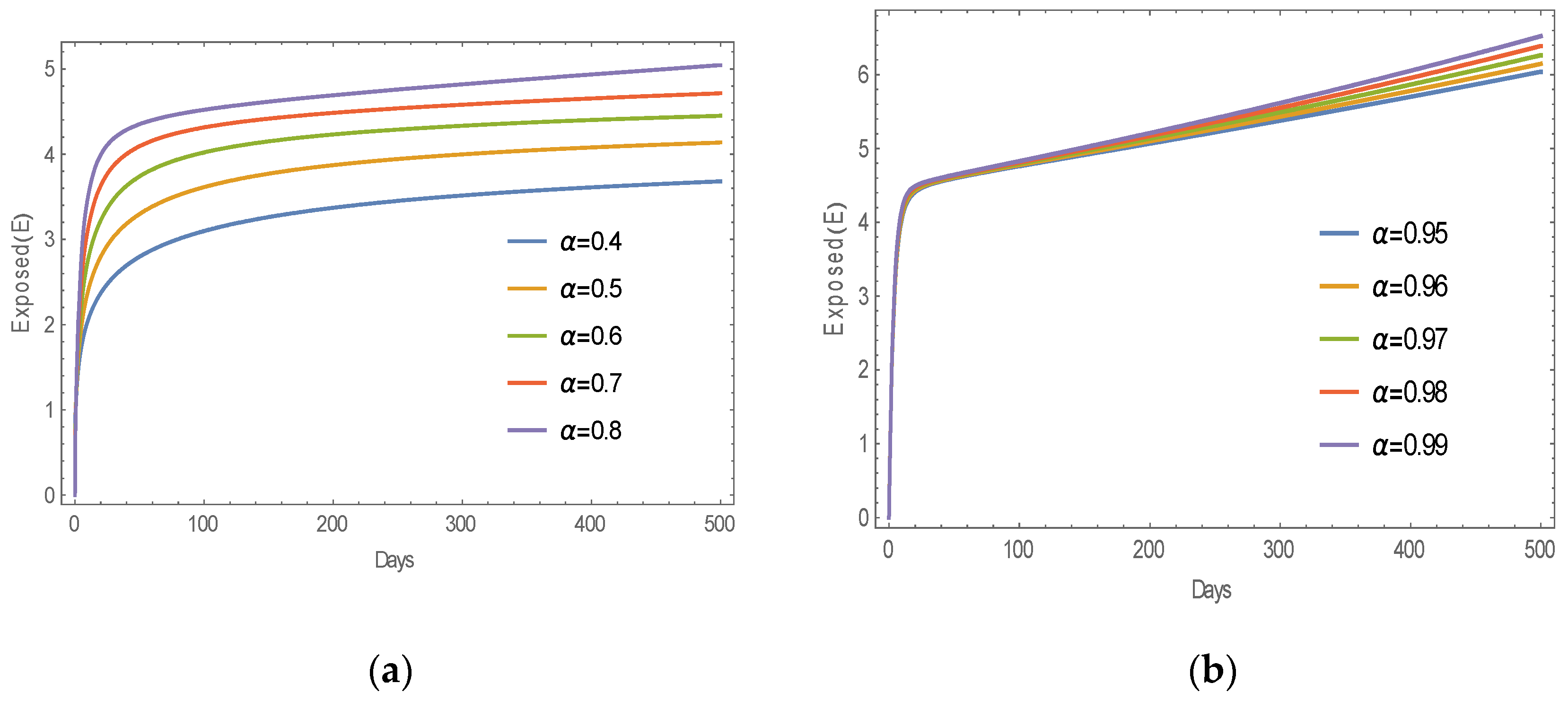
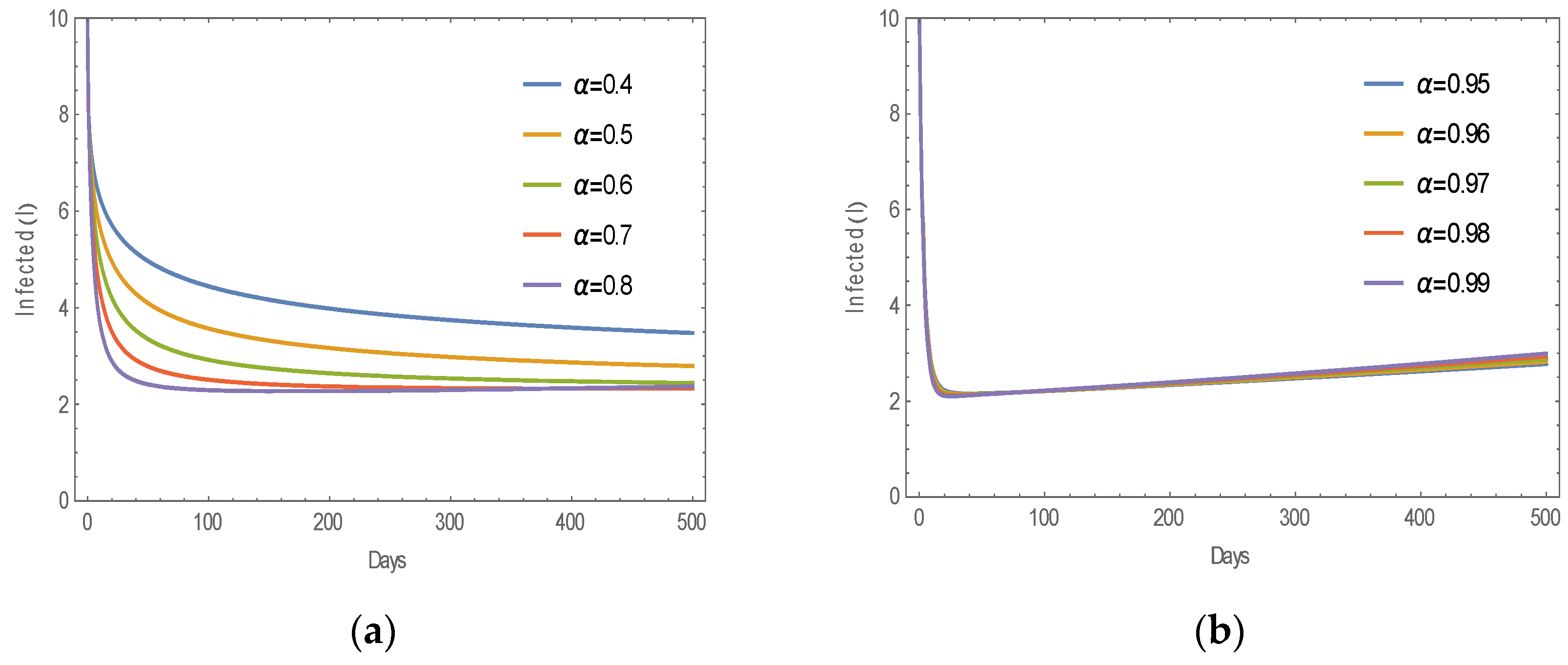
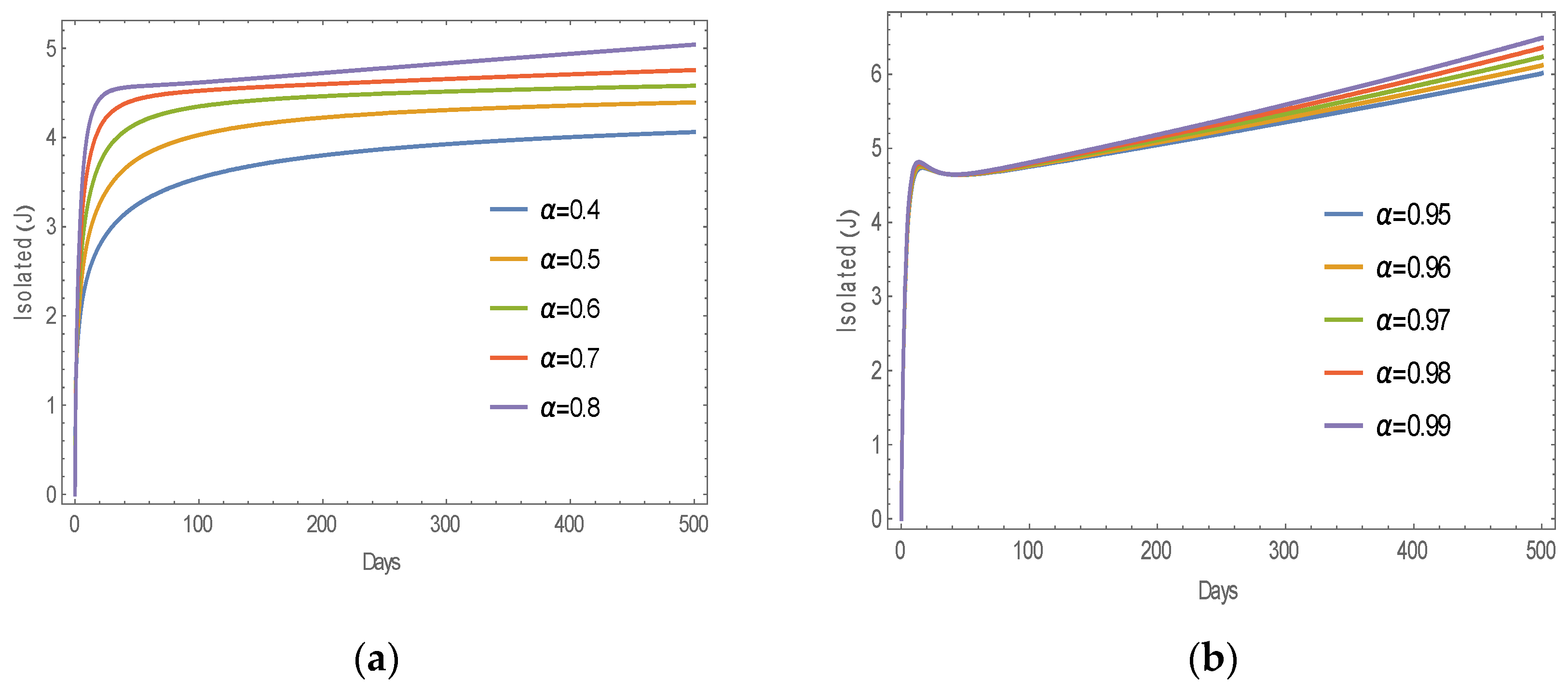
6. Numerical Results

6.1. Numerical Simulation of MERS

This subsection presents numerical results and simulations of MERS. To achieve that, we consider the parameter values, as in

Table 1. Parameter values for proposed system.

Parameter	Parameter Value	Unit	Source
${\sigma }_1$	$0.0433$	1/day	Nofe et al. [4]
${\sigma }_2$	$0.0457$	1/day	Estimated
$\mu$	$0.000034$	1/day	Nofe et al. [4]
$\gamma$	$0.1501$	1/day	Nofe et al. [4]
$d_1$	$0.0294$	1/day	Nofe et al. [4]
$d_2$	$0.0227$	1/day	Nofe et al. [4]
$\beta$	$0.122$	1/day	Nofe et al. [4]
${ϵ}_E$	$0.2996$	-	Nofe et al. [4]
${ϵ}_J$	$0.0899$	-	Nofe et al. [4]
$\mathrm{{\rm K}}$	$0.1026$	1/day	Nofe et al. [4]
$P$	$170$	individual/day	Nofe et al. [4]

and the initial values (Nofe et al. [4]) $S_0=\mathrm{4,999,990}$, $E_0=0$, $I_0=10$, $J_0=0$, and $R_0=0$. Wolfram Mathematica was used to compute all the approximate solutions with $\chi =0.99$.

Regarding the parameter values in Table 1, the ${\mathcal{R}}_c=1.011363>1$. Then, there exists a unique endemic equilibrium, $E_{*}=\left(\mathrm{4,913,405}, 29,13, 29,55,761\right),$ and the point of the model (10) is positive, which is locally asymptotically stable. The ${\mathcal{R}}_0=2.03292>1$. Then, the disease-free equilibrium of (10) is locally asymptotically unstable.

Comparisons among the numerical results are introduced in

Table 2. Approximate solutions of S$\left(t\right)$ at different time intervals.

	$\mathit{\alpha }=0.4$		$\mathit{\alpha }=0.6$		$\mathit{\alpha }=0.8$
$\mathit{t}$	MVM	ITM	MVM	ITM	MVM	ITM
$\mathbf{0}$	$\mathrm{4,999,990}$	$\mathrm{4,999,990}$	$\mathrm{4,999,990}$	$\mathrm{4,999,990}$	$\mathrm{4,999,990}$	$\mathrm{4,999,990}$
$\mathbf{50}$	$\mathrm{4,999,985}$	$\mathrm{4,999,985}$	$\mathrm{4,999,982}$	$\mathrm{4,999,982}$	$\mathrm{4,999,975}$	$\mathrm{4,999,975}$
$\mathbf{100}$	$\mathrm{4,999,984}$	$\mathrm{4,999,984}$	$\mathrm{4,999,979}$	$\mathrm{4,999,979}$	$\mathrm{4,999,967}$	$\mathrm{4,999,967}$
$\mathbf{150}$	$\mathrm{4,999,984}$	$\mathrm{4,999,984}$	$\mathrm{4,999,976}$	$\mathrm{4,999,976}$	$\mathrm{4,999,959}$	$\mathrm{4,999,959}$
$\mathbf{200}$	$\mathrm{4,999,983}$	$\mathrm{4,999,983}$	$\mathrm{4,999,974}$	$\mathrm{4,999,974}$	$\mathrm{4,999,951}$	$\mathrm{4,999,951}$
$\mathbf{250}$	$\mathrm{4,999,983}$	$\mathrm{4,999,983}$	$\mathrm{4,999,973}$	$\mathrm{4,999,973}$	$\mathrm{4,999,944}$	$\mathrm{4,999,944}$
$\mathbf{300}$	$\mathrm{4,999,982}$	$\mathrm{4,999,982}$	$\mathrm{4,999,971}$	$\mathrm{4,999,971}$	$\mathrm{4,999,937}$	$\mathrm{4,999,937}$
$\mathbf{350}$	$\mathrm{4,999,982}$	$\mathrm{4,999,982}$	$\mathrm{4,999,969}$	$\mathrm{4,999,969}$	$\mathrm{4,999,930}$	$\mathrm{4,999,930}$
$\mathbf{400}$	$\mathrm{4,999,982}$	$\mathrm{4,999,982}$	$\mathrm{4,999,968}$	$\mathrm{4,999,968}$	$\mathrm{4,999,923}$	$\mathrm{4,999,923}$
$\mathbf{450}$	$\mathrm{4,999,981}$	$\mathrm{4,999,981}$	$\mathrm{4,999,966}$	$\mathrm{4,999,966}$	$\mathrm{4,999,917}$	$\mathrm{4,999,917}$
$\mathbf{500}$	$\mathrm{4,999,981}$	$\mathrm{4,999,981}$	$\mathrm{4,999,965}$	$\mathrm{4,999,965}$	$\mathrm{4,999,910}$	$\mathrm{4,999,910}$

,

Table 3. Approximate solutions of $E\left(t\right)$ at different time intervals.

	$\mathit{\alpha }=0.4$		$\mathit{\alpha }=0.6$		$\mathit{\alpha }=0.8$
$\mathit{t}$	MVM	ITM	MVM	ITM	MVM	ITM
$\mathbf{0}$	0	0	0	0	0	0
$\mathbf{50}$	$2.7963$	$2.7960$	$3.7385$	$3.7347$	$4.3512$	$4.3488$
$\mathbf{100}$	$3.0979$	$3.0981$	$4.0200$	$4.0186$	$4.5201$	$4.5196$
$\mathbf{150}$	$3.2614$	$3.2617$	$4.1502$	$4.1494$	$4.6154$	$4.6152$
$\mathbf{200}$	$3.3708$	$3.3712$	$4.2310$	$4.2305$	$4.6907$	$4.6906$
$\mathbf{250}$	$3.4517$	$3.4520$	$4.2886$	$4.2883$	$4.7573$	$4.7573$
$\mathbf{300}$	$3.5157$	$3.5160$	$4.3332$	$4.3329$	$4.8190$	$4.8191$
$\mathbf{350}$	$3.5669$	$3.5672$	$4.3695$	$4.3693$	$4.8777$	$4.8778$
$\mathbf{400}$	$3.6104$	$3.6107$	$4.4002$	$4.4001$	$4.9344$	$4.9345$
$\mathbf{450}$	$3.6477$	$3.6480$	$4.4269$	$4.4268$	$4.9895$	$4.9897$
$\mathbf{500}$	$3.6803$	$3.6806$	$4.4506$	$4.4506$	$5.0436$	$5.0438$

,

Table 4. Approximate solutions of I$\left(t\right)$ at different time intervals.

	$\mathit{\alpha }=0.4$		$\mathit{\alpha }=0.6$		$\mathit{\alpha }=0.8$
$\mathit{t}$	MVM	ITM	MVM	ITM	MVM	ITM
$\mathbf{0}$	10	10	10	10	10	10
$\mathbf{50}$	$4.9648$	$4.9655$	$3.3488$	$3.3558$	$2.4119$	$2.4158$
$\mathbf{100}$	$4.4429$	$4.4428$	$2.9193$	$2.9220$	$2.2920$	$2.2929$
$\mathbf{150}$	$4.1645$	$4.1642$	$2.7416$	$2.7430$	$2.2703$	$2.2707$
$\mathbf{200}$	$3.9808$	$3.9803$	$2.6423$	$2.6432$	$2.2714$	$2.2717$
$\mathbf{250}$	$3.8465$	$3.8460$	$2.5784$	$2.5791$	$2.2814$	$2.2816$
$\mathbf{300}$	$3.7422$	$3.7417$	$2.5338$	$2.5344$	$2.2957$	$2.2959$
$\mathbf{350}$	$3.6578$	$3.6574$	$2.5010$	$2.5014$	$2.3124$	$2.3126$
$\mathbf{400}$	$3.5876$	$3.5872$	$2.4759$	$2.4763$	$2.3306$	$2.3307$
$\mathbf{450}$	$3.5279$	$3.5275$	$2.4562$	$2.4565$	$2.3497$	$2.3498$
$\mathbf{500}$	$3.4762$	$3.4758$	$2.4404$	$2.4407$	$2.3695$	$2.3696$

,

Table 5. Approximate solutions of J$\left(t\right)$ at different time intervals.

	$\mathit{\alpha }=0.4$		$\mathit{\alpha }=0.6$		$\mathit{\alpha }=0.8$
$\mathit{t}$	MVM	ITM	MVM	ITM	MVM	ITM
$\mathbf{0}$	0	0	0	0	0	0
$\mathbf{50}$	$3.2438$	$3.2429$	$4.1545$	$4.1505$	$4.5712$	$4.5706$
$\mathbf{100}$	$3.5444$	$3.5442$	$4.3458$	$4.3446$	$4.6147$	$4.6149$
$\mathbf{150}$	$3.6989$	$3.6989$	$4.4191$	$4.4185$	$4.6666$	$4.6668$
$\mathbf{200}$	$3.7982$	$3.7983$	$4.4614$	$4.4608$	$4.7214$	$4.7215$
$\mathbf{250}$	$3.8694$	$3.8695$	$4.4904$	$4.4902$	$4.7762$	$4.7763$
$\mathbf{300}$	$3.9237$	$3.9243$	$4.5133$	$4.5132$	$4.8302$	$4.8303$
$\mathbf{350}$	$3.9671$	$3.9672$	$4.5324$	$4.5324$	$4.8834$	$4.8836$
$\mathbf{400}$	$4.0028$	$4.0029$	$4.54919$	$4.5491$	$4.9360$	$4.9361$
$\mathbf{450}$	$4.0329$	$4.0330$	$4.5642$	$4.5642$	$4.9879$	$4.9881$
$\mathbf{500}$	$4.0588$	$4.0589$	$4.5780$	$4.5780$	$5.0394$	$5.0396$

and

Table 6. Approximate solutions of R$\left(t\right)$ at different time intervals.

	$\mathit{\alpha }=0.4$		$\mathit{\alpha }=0.6$		$\mathit{\alpha }=0.8$
$\mathit{t}$	MVM	ITM	MVM	ITM	MVM	ITM
$\mathbf{0}$	0	0	0	0	0	0
$\mathbf{50}$	$1.9809$	$1.9859$	$4.0560$	$4.0596$	$8.0843$	$8.0860$
$\mathbf{100}$	$2.5509$	$2.5559$	$5.9402$	$5.9442$	$13.639$	$13.642$
$\mathbf{150}$	$2.9576$	$2.9626$	$7.4453$	$7.4495$	$18.675$	$18.678$
$\mathbf{200}$	$3.2853$	$3.2903$	$8.7527$	$8.7570$	$23.436$	$23.441$
$\mathbf{250}$	$3.5646$	$3.5696$	$9.9329$	$9.9372$	$28.022$	$28.026$
$\mathbf{300}$	$3.8108$	$3.8158$	$11.022$	$11.026$	$32.483$	$32.488$
$\mathbf{350}$	$4.0325$	$4.0374$	$12.051$	$12.046$	$36.852$	$36.857$
$\mathbf{400}$	$4.2351$	$4.2401$	$13.006$	$13.020$	$41.150$	$41.156$
$\mathbf{450}$	$4.4226$	$4.4275$	$13.925$	$13.930$	$45.393$	$45.399$
$\mathbf{500}$	$4.5975$	$4.6025$	$14.806$	$14.811$	$49.591$	$49.598$

, with $k=0.5$, which show that the numerical results of the MVM and ITM are very similar. This helps us see how MERS has evolved as a behavior. The arbitrary-order MERS model offers greater flexibility, as demonstrated by the behavior of the solutions for susceptible $S\left(t\right)$, exposed $E\left(t\right)$, infected $I\left(t\right)$, isolated $J\left(t\right)$, and recovered $R\left(t\right)$ over time $t$. This is illustrated in Figure 1, Figure 2, Figure 3, Figure 4 and Figure 5: part (a) shows distinct values of $\alpha$, while part (b) depicts larger values of $\alpha$ approaching 1. Furthermore, we deduced from these plots that the outcome of the model under consideration is contingent upon its past performance as well as the parameters specified in the system (10). A comparison of the plots shows that the functions produced from both forms of derivatives behave consistently, even though the resultant values are different. The simulation of the numerical solution for infected I(t) is slower with time, as shown in Figure 2. Based on the results obtained, it can be observed that the proposed scheme facilitates the understanding of behavior using fractional derivatives.

Remark 3.

We used Wolfram Mathematica to extract the integer part of the values for $S\left(t\right)$ in Table 2.

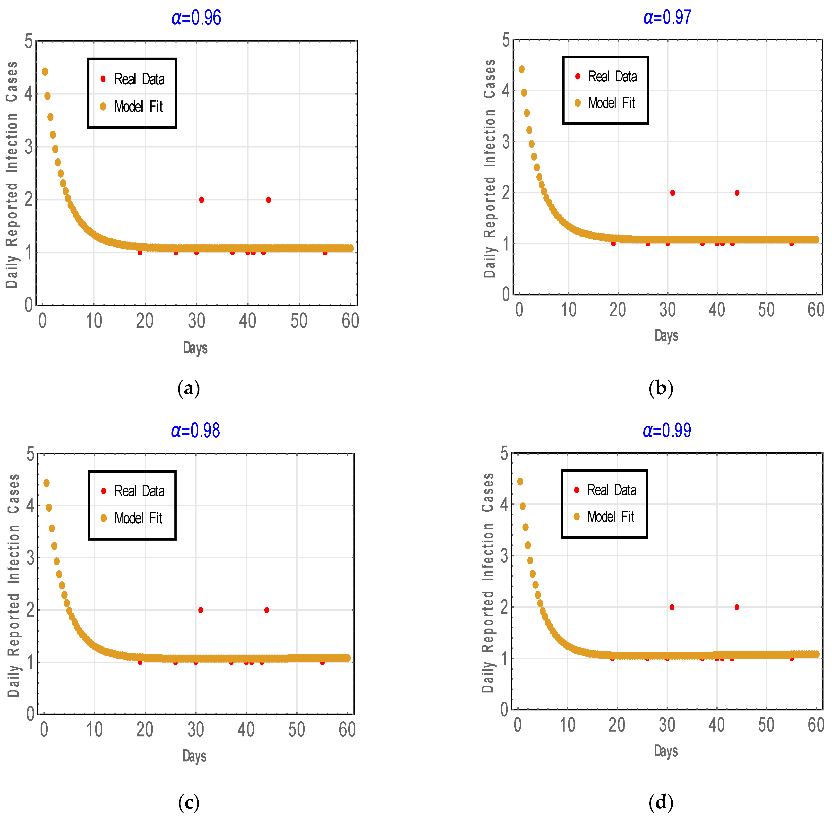
6.2. Fitting Model to Real Data

This subsection presents the fitting of the MERS model to real data. To achieve this, we considered the parameter values in Table 1. The initial value of $S_0=\mathrm{6,218,000}$ was the population of Riyadh, Saudi Arabia, in late 2015 [32], $E_0=0$, $I_0=5$, $J_0=0$, and $R_0=0$. Wolfram Mathematica was used to compute all the approximate solutions with $\chi =0.99$ and $k=0.5$.

We utilized real data from Riyadh, Saudi Arabia, in 2015 with laboratory-confirmed cases of MERS infection, as detailed in

Table 7. Real data on laboratory-confirmed cases of MERS infection.

Day	Reported MERS Cases
19 September 2015	$1$
26 September 2015	$1$
30 September 2015	$1$
1 October 2015	$2$
7 October 2015	$1$
10 October 2015	$1$
11 October 2015	$1$
13 October 2015	$1$
14 October 2015	$2$
22 October 2015	$1$

[33]. A comparison of reported MERS cases with model fittings is presented in Figure 6 and Figure 7. These figures show an excellent match with the real data. Our findings suggest that fractional-order models provide a variety of fitting data compared to traditional integer-order models.

7. Conclusions

In this work, we have presented a fractional-order derivative model and analyzed it for the MERS model. Utilizing the fixed-point theorem, we have established the existence and uniqueness of the solution to the proposed model. We employed the implicit trapezoidal and the mean value theorem methods to solve the fractional model suggested in the sense of Caputo. Furthermore, we studied the stability of our methods and demonstrated that these methods are stable. Fractional calculus theory can be used to adequately simulate the MERS model’s dynamic behavior, which is dependent on both the current time and its history. We have created a stronger and more accurate model by including Caputo fractional derivatives. To sum up, the methods suggested are quite methodical and efficient, providing workable ways to investigate nonlinear fractional mathematical models that explain biological processes. In the area of mathematical modeling, the use of fractional calculus presents novel ideas.

References

1. WHO. Available online: https://www.who.int/news-room/fact-sheets/detail/middle-east-respiratory-syndrome-coronavirus-(mers-cov)?gad_source=1&gclid=Cj0KCQjwmMayBhDuARIsAM9HM8c1PPHDJWHIKsKn146_w6EYp7Rnza8cbhHUKd1qO-OcN7KFiOR6Yj8aAkBAEALw_wcB (accessed on 1 August 2024).
2. El-Saka HA, A.; Obaya, I.; Lee, S.; Jang, B. Fractional model for Middle East respiratory syndrome coronavirus on a complex heterogeneous network. Sci. Rep. 2022, 12, 24–25. [Google Scholar] [CrossRef] [PubMed]
3. Elkholy, A.A.; Grant, R.; Assiri, A.; Elhakim, M.; Malik, M.R.; Van Kerkhove, M.D. MERS-CoV infection among healthcare workers and risk factors for death: Retrospective analysis of all laboratory-confirmed cases reported to WHO from 2012 to 2 June 2018. J. Infect. Public Health 2020, 13, 418–422. [Google Scholar] [CrossRef] [PubMed]
4. Al-Asuoad, N.; Rong, L.; Alaswad, S.; Shillor, M. Mathematical model and simulations of MERS outbreak: Predictions and implications for control measures. BIOMATH 2017, 5, 1612141. [Google Scholar] [CrossRef]
5. Arafa AA, M.; Rida, S.Z.; Khalil, M. Fractional modeling dynamics of HIV and CD4+ T-cells during primary infection. Nonlinear Biomed. Phys. 2012, 6, 1. [Google Scholar] [CrossRef]
6. Sweilam, N.H.; Nagy, A.M.; Elfahri, L.E. Fractional-order delayed Salmonella transmission model: A numerical simulation. Progr. Fract. Differ. Appl. 2022, 8, 63–76. [Google Scholar]
7. Khalil, M.; Arafa, A.; Sayed, A. On a Fractional Variable-Order Model of MERS-CoV. Prog. Fract. Differ. Appl. 2023, 9, 331–344. [Google Scholar]
8. Chechkin, A.V.; Gorenflo, R.; Sokolov, I.M. Fractional diffusion in inhomogeneous media. J. Phys. A. Math. Gen. 2005, 38, L679. [Google Scholar] [CrossRef]
9. Monje, C.A.; Chen, Y.; Vinagre, B.M.; Xue, D.; Feliu-Batlle, V. Fractional-Order Systems and Controls: Fundamentals and Applications; Springer Science & Business Media: Berlin/Heidelberg, Germany, 2010. [Google Scholar]
10. Hadhoud, A.R.; Abd Alaal, F.E.; Abdelaziz, A.A.; Radwan, T. A Cubic Spline Collocation Method to Solve a Nonlinear Space-Fractional Fisher’s Equation and Its Stability Examination. Fractal Fract. 2022, 6, 470. [Google Scholar] [CrossRef]
11. Hadhoud, A.R.; Abd Alaal, F.E.; Abdelaziz, A.A. On the numerical investigations of the time-fractional modified Burgers’ equation with conformable derivative, and its stability analysis. J. Math. Comput. Sci. 2021, 12, 36. [Google Scholar]
12. Azhar, E.I.; Hui, D.S.C.; Memish, Z.A.; Drosten, C.; Zumla, A. The middle east respiratory syndrome (MERS). Infect. Dis. Clin. 2019, 33, 891–905. [Google Scholar] [CrossRef]
13. Chowell, G.; Abdirizak, F.; Lee, S.; Lee, J.; Jung, E.; Nishiura, H.; Viboud, C. Transmission characteristics of MERS and SARS in the healthcare setting: A comparative study. BMC Med. 2015, 13, 210. [Google Scholar] [CrossRef] [PubMed]
14. World Health Organization. WHO MERS Global Summary and Assessment of Risk; World Health Organization: Geneva, Switzerland, 2019.
15. Tahir, M.; Shah SI, A.; Zaman, G.; Khan, T. Stability behaviour of mathematical model MERS corona virus spread in population. Filomat 2019, 33, 3947–3960. [Google Scholar] [CrossRef]
16. Tahir, M.; Ali Shah, S.I.; Zaman, G.; Khan, T. A dynamic compartmental mathematical model describing the transmissibility of MERS-CoV virus in public. Punjab Univ. J. Math. 2020, 51, 51–71. [Google Scholar]
17. Liang, K. Mathematical model of infection kinetics and its analysis for COVID-19, SARS and MERS. Infect. Genet. Evol. 2020, 82, 104306. [Google Scholar] [CrossRef] [PubMed]
18. DarAssi, M.H.; Shatnawi, T.A.M.; Safi, M.A. Mathematical analysis of a MERS-Cov coronavirus model. Demonstr. Math. 2022, 55, 265–276. [Google Scholar] [CrossRef]
19. Dighe, A.; Jombart, T.; Van Kerkhove, M.; Ferguson, N. A mathematical model of the transmission of middle East respiratory syndrome coronavirus in dromedary camels (Camelus dromedarius). Int. J. Infect. Dis. 2019, 79, 1. [Google Scholar] [CrossRef]
20. Chang, H.J. Estimation of basic reproduction number of the Middle East respiratory syndrome coronavirus (MERS-CoV) during the outbreak in South Korea, 2015. Biomed. Eng. Online 2017, 16, 79. [Google Scholar] [CrossRef]
21. Mackay, I.M.; Arden, K.E. MERS coronavirus: Diagnostics, epidemiology and transmission. Virol. J. 2015, 12, 222. [Google Scholar] [CrossRef]
22. Samko, S.G.; Kilbas, A.A.; Marichev, O.I. Fractional Integrals and Derivatives; Gordon and Breach: London, UK, 1993. [Google Scholar]
23. Diethelm, K.; Ford, N.J. The Analysis of Fractional Differential Equations; Lecture Notes in Mathematics; Springer: Berlin/Heidelberg, Germany, 2010; Volume 2004. [Google Scholar] [CrossRef]
24. Li, C.; Zeng, F. The finite difference methods for fractional ordinary differential equations. Numer. Funct. Anal. Optim. 2013, 34, 149–179. [Google Scholar] [CrossRef]
25. Gumel, A.B.; Ruan, S.; Day, T.; Watmough, J.; Brauer, F.; Driessche, P.v.D.; Gabrielson, D.; Bowman, C.; Alexander, M.E.; Ardal, S.; et al. Modelling strategies for controlling SARS outbreaks. Proc. R. Soc. B Biol. Sci. 2004, 271, 2223–2232. [Google Scholar] [CrossRef]
26. Agarwal, P.; Ramadan, M.A.; Rageh, A.A.M.; Hadhoud, A.R. A fractional-order mathematical model for analyzing the pandemic trend of COVID-19. Math. Methods Appl. Sci. 2022, 45, 4625–4642. [Google Scholar] [CrossRef] [PubMed]
27. Rezapour, S.; Mohammadi, H. A study on the AH1N1/09 influenza transmission model with the fractional Caputo–Fabrizio derivative. Adv. Differ. Equ. 2020, 2020, 488. [Google Scholar] [CrossRef]
28. Tuan, N.H.; Mohammadi, H.; Rezapour, S. A mathematical model for COVID-19 transmission by using the Caputo fractional derivative. Chaos Solitons Fractals 2020, 140, 110107. [Google Scholar] [CrossRef] [PubMed]
29. Burden, R.L.; Faires, J.D. Numerical Analysis, 8th ed.; Thomson Brooks/Cole: Belmont, CA, USA, 2005. [Google Scholar]
30. Hadhoud, A.R.; Alaal, F.E.A.; Abdelaziz, A.A.; Radwan, T. Numerical treatment of the generalized time—Fractional Huxley—Burgers’ equation and its stability examination. Demonstr. Math. 2021, 54, 436–451. [Google Scholar] [CrossRef]
31. Hadhoud, A.R.; Gaafar, F.M.; Alaal, F.E.A.; Abdelaziz, A.A.; Boulaaras, S.; Radwan, T. A Robust Collocation Method for Time Fractional PDEs Based on Mean Value Theorem and Cubic B-Splines. Partial Differ. Equ. Appl. Math. 2024, in press. [Google Scholar] [CrossRef]
32. MacroTrends. Available online: https://www.macrotrends.net/globalmetrics/cities/22432/riyadh/population#google_vignette (accessed on 1 August 2024).
33. Van Kerkhove, M.D.; Alaswad, S.; Assiri, A.; Perera, R.A.; Peiris, M.; El Bushra, H.E.; BinSaeed, A.A. Transmissibility of MERS-CoV infection in closed setting, Riyadh, Saudi Arabia, 2015. Emerg. Infect. Dis. 2019, 25, 1802–1809. [Google Scholar] [CrossRef]
Figure 1. Graph depicting approximate solutions of S(t) part (a) displays results for distinct values of α, while part (b) shows results for larger values of α approaching 1.
Fractalfract 08 00521 g001
Figure 2. Graph depicting approximate solutions of E t , part (a) displays results for distinct values of α, while part (b) shows results for larger values of α approaching 1.
Fractalfract 08 00521 g002
Figure 3. Graph depicting approximate solutions of I t , part (a) displays results for distinct values of α, while part (b) shows results for larger values of α approaching 1.
Fractalfract 08 00521 g003
Figure 4. Graph depicting approximate solutions of J t , part (a) displays results for distinct values of α, while part (b) shows results for larger values of α approaching 1.
Fractalfract 08 00521 g004
Figure 5. Graph depicting approximate solutions of R t , part (a) displays results for distinct values of α, while part (b) shows results for larger values of α approaching 1.
Fractalfract 08 00521 g005
Figure 6. Comparison of reported MERS cases in Riyadh, Saudi Arabia, with model fitting at various values of α , part (a) shows α = 0.5 , (b) shows α = 0.6 , (c) shows α = 0.7 , and (d) shows α = 0.8 .
Fractalfract 08 00521 g006
Figure 7. Comparison of Reported MERS Cases in Riyadh, Saudi Arabia, with model fitting at various values of α , part (a) shows α = 0.96 , (b) shows α = 0.97 , (c) shows α = 0.98 , and (d) shows α = 0.99 .
Fractalfract 08 00521 g007