Abstract
Fractional cointegration in time series data has been explored by several authors, but panel data applications have been largely neglected. A previous study of ours discovered that the Chen and Hurvich fractional cointegration test for time series was fairly robust to a moderate degree of heterogeneity across sections of the six tests considered. Therefore, this paper advances a customized version of the Chen and Hurvich methodology to detect cointegrating connections in panels with unobserved fixed effects. Specifically, we develop a test statistic that accommodates variation in the long-term cointegrating vectors and fractional cointegration parameters across observational units. The behavior of our proposed test is examined through extensive Monte Carlo experiments under various data-generating processes and circumstances. The findings reveal that our modified test performs quite well comparatively and can successfully identify fractional cointegrating relationships in panels, even in the presence of idiosyncratic disturbances unique to each cross-sectional unit. Furthermore, the proposed modified test procedure established the presence of long-run equilibrium between the exchange rate and labor wage of 36 countries’ agricultural markets.
MSC:
94A08; 68U10
1. Introduction
While cointegration techniques have proven useful in economic and financial research for decades in examining equilibrium relationships between non-stationary time series data, the ability of fractional cointegration to accommodate non-integer degrees of integration and additional nonstationary elements addresses the limitations of traditional approaches. Fractional cointegration relaxes assumptions regarding integration orders and potential randomness in time series, allowing for more robust modelling. As econometric tools progress to incorporate more complex real-world variations, fractional techniques lend increased accuracy to describing equilibrium conditions over time. Continued exploration of fractional specifications holds promise for deeper insights into the dynamics between financial and economic variables [1,2,3]. The complex research surrounding fractional cointegration in multivariate time series has led to an abundance of assessment techniques for detecting such interdependencies. A wealth of studies have created and evaluated various statistical approaches for testing fractional cointegration, ranging from early explorations that provided foundational methods to more recent innovations that have built upon previous work. Among the many contributions to this area of inquiry are tests proposed by Johansen and Nielsen [1], Marmol and Velasco [4], Chen and Hurvich [5], Johansen [6], Robinson [7], Nielsen [8], Avarucci and Velasco [9], Łasak [10], Johansen and Nielsen [11], Souza et al. [12]—each offering novel ways of quantifying the perplexing dynamics within nonstationary data comprised of multiple correlated components evolving through fractal processes over time.
Leschinski et al. [13] uncovered substantial shortcomings in how some fractional cointegration tests operate with limited data, as evidenced by their thorough Monte Carlo analysis of these methods with time series. Certain procedures demonstrated weak detection abilities or skewed false-positive rates when short-run elements were interrelated. This generalization covered the strategies put forth by Nielsen and Shimotsu [14], Nielsen and Shimotsu [14] (or Robinson and Yajima [15]), Marmol and Velasco [4], and Hualde and Velasco [16]. While investigating spurious test outcomes with confined samples, their work highlighted necessary improvements for robust evaluation of cointegrated associations over the long term.
Thus, this paper builds on the conceptual framework that is based on the foundational role of cointegration techniques in economic and financial research, focusing on fractional cointegration, which improves traditional models by allowing for non-integer degrees of integration and capturing more complex, non-linear dynamics in time series data. Furthermore, in the previous work by Olaniran and Ismail [17], the author specifically focused on determining the appropriateness of the existing fractional cointegration test for the fixed effects panel model. The Chen and Hurvich fractional cointegration test [5] originally developed for time series data was observed to withstand a moderate level of cross-sectional heterogeneity. Therefore, in this paper, we modified the test procedure to fully accommodate the fixed effect fractional cointegration structure in panel data.
2. Related Work
Both fractional and standard cointegration were defined concurrently by Engle and Granger [18], but standard cointegration has received significantly more attention. As a result, there has been a need to focus heavily on fractional cointegration in recent years due to the paucity of research, particularly for panel data as opposed to time series data.
Panel data analysis is a means of investigating a specific subject across numerous places over a fixed length of time, which is becoming increasingly popular among social and behavioural science academics. Panel data combine time series and cross-sections to improve data quality and quantity in ways that would be impossible if only one of these two dimensions were utilized [19].
Standard cointegration only allows integer values for the memory parameters
and
, and unit root theory is used to test for cointegration’s existence. The fractional cointegration framework, on the other hand, is more general, because it enables fractional values for the memory parameter and any positive real number for
. As indicated by the work of [5,7,20], fractional cointegration recently received significant attention. For time series data, all of these publications assume that the observed series is either bivariate or that the cointegrating rank is one.
Robinson [21] observed that in the presence of a correlation between
and
, the OLS estimator will be inconsistent, and they proposed a narrowband least-squares estimator (NBLSE) of the long memory parameter in the frequency domain, which was further studied in Marinucci and Robinson [20]. Robinson and Yajima [15] presented methods for finding the cointegrating rank, as in Chen and Hurvich [5], which focused on the estimation of the space of cointegrating vectors without emphasizing the use of time and cross-sections.
While Chen and Hurvich [22] tapered a narrowband least-squares estimator of the cointegration parameter utilizing a family of tapers, alternative approaches exist. Their methodology changed the data
times to account for potential
th order polynomial trends, rendering the resultant estimator insensitive to deterministic polynomial trends within the series. However, other scholars propose directly modeling such trends to comparable effects. After changing these parameters, they propose multiplying the data by a tapered sequence of constants that are dependent on the positive integer p to emphasize more recent observations. Yet, some argue for applying non-linear tapers or transforming variables prior to estimation to better address non-stationarities. In short, while their proposal offers one valid method, room remains to explore complementary techniques addressing cointegration under non-stationary conditions.
Chen and Hurvich [5] developed an innovative test for fractional cointegration based on their multivariate common-components model, allowing memory parameters to vary across factors. This novel approach recognizes that the cointegrating rank may exceed one, with the original vectors split into orthogonal fractional subspaces, yielding errors with fluctuating memory attributes from vectors drawn across different subspaces. Their fractional cointegration technique using a common-components structure with changeable memory dynamics across factors proved insightful for assessing long-run relationships between nonstationary series. Also, the complex relationships shared between financial variables often emerge through time. Resolving these intricate connections requires parsing cointegrating residuals to uncover the inherent long-term patterns. By applying a Gaussian semiparametric approach using an appropriately scaling bandwidth, one can derive a stable gauge of the persistence inherently linking economic factors within a specified cointegrating framework. With this metric in hand, we can neatly isolate cointegrating subsets and rigorously examine whether fractional processes underlie the observed synchronization. Such techniques help bring order to the initially chaotic web of interdependencies that defines economic landscapes.
Ergemen and Velasco [23] explored a large dataset with numerous variables and time periods using a panel data model containing fixed factors that enable cross-sectional interdependence, persistent information, and fractionally built-in inaccuracies. Their investigation gives a broad analysis for stationary and non-stationary signs, as corroborated through Monte Carlo tests that exhibited effectiveness in implementation. As suggested in a prior study by Robinson and Velasco [24], the strategy was further expanded to alternative estimation methods involving fixed effects and the generalized method of moments: a technique applying instruments to acquire consistent and proficient estimates from unobservable variables.
Idiosyncratic shocks can be utilized to highlight spatial dependency in a broader model by permitting nonfactor endogeneity, which results in a cointegrated system analysis in the traditional sense, as in Ergemen [25]. By comparing mean group estimates with pooled estimates produced from a homogeneous version of the model, panel unit-root and related hypothesis testing, as well as slope parameter homogeneity tests, could be constructed.
Leschinski et al. [13] explored fractional cointegration across various econometric approaches. Nine fractional cointegration tests evaluating spectral density and residual-based methods were compared. When short-term influences contained interdependences, several techniques uncovered noticeably amplified sizes. Their efficacy diverged as well, with power varying between common-component frameworks opposite triangular systems. Overall, the analysis illuminated how the presence of interconnected transient elements impacts the performance of fractional cointegration testing procedures. It was also found that the effectiveness of the test procedures diverged substantially between the two modeling situations. The test procedure of Chen and Hurvich [5] specifically had considerably higher power for stationary systems under the common component specification, whereas the techniques of Robinson and Yajima [15] and Hualde and Velasco [16] proved to be less able to identify fractional cointegration. In contrast, the test by Chen and Hurvich [5] strongly determined cointegrating associations assuming steady components, and the methodology of Robinson and Yajima [15] and that of Hualde and Velasco [16] saw diminishing prospects for detecting fractional cointegrating connections.
The methods proposed by Robinson [7], Nielsen [8], and Zhang et al. [26] are well-regarded for their robustness to short-term correlation and their simplicity, making them appealing for various applications. However, none of these works presented a comprehensive test for fractional integration and cointegration that was broadly applicable across all types of panel data, particularly in contexts involving heterogeneity. Olaniran and Ismail [17] addressed this gap by evaluating existing fractional cointegration tests in the context of time series data, focusing on their effectiveness for panel data with fixed effects and moderate to high heterogeneity. Among the methods reviewed, only Chen and Hurvich [5] proved to be effective under such conditions.
This paper builds on Olaniran and Ismail [17] by further refining Chen and Hurvich [5]’s test to accommodate fractional cointegration in fixed effect panel data that exhibit varying degrees of heterogeneity across observational units. Compared to prior studies, the unique contribution of this work lies in its ability to address fractional cointegration more comprehensively in diverse panel data settings, filling a critical gap in the literature. While previous methodologies are valuable, they fall short in contexts of significant heterogeneity, which is increasingly relevant in empirical economic and financial applications. By enhancing Chen and Hurvich [5]’s test for a wider range of panel data, this paper contributes an essential tool for researchers dealing with fractional cointegration in complex datasets, advancing the methodological landscape in this area.
3. Modified Chen and Hurvich [5] Test for Fixed Effects Panel Model
Consider a balanced panel model with fixed effects estimating cointegration relationships. The model examines the long-run equilibrium between variables across
individual units over
time periods, creating a full sample of
observations. The model is defined as follows:
This framework assumes a constant cointegrating parameter
linking independent variables
and dependent variables
for all
individuals. The model controls for individual-specific characteristics through fixed-effects parameters
. Fractional cointegration exists if two conditions are met. First, the independent and dependent variables share a common stochastic trend, making them nonstationary yet moving together in the long run. Second, their linear combination is stationary, implying convergence to equilibrium in the error correction form. Proper specification requires testing the orders of integration to validate the theoretical underpinnings of the cointegrating relationship. Overall, this approach explores how divergences from long-run steady states across units are self-correcting over repeated time periods. The null hypothesis
of no fractional cointegration holds if
, whereas the alternative of cointegration is supported if
.
The bivariate system described in (1) can be simplified to the Phillips [27] classical cointegration model if
equals 0 and
is equal to 1, known as
. The fractional lag operator
is derived using
, where the Gamma function
is defined as
.
Equation (1) can be represented as follows:
If we let
, we have the following:
It is evident that from the demeaning applied to Equation (1), Equation (3) removes the individual cross-sectional parameters
from the original model, consequently simplifying the time series representation. As elucidated by Chen and Hurvich [5], the revised formulation within Equation (3) allows for estimation using the tapered narrow-band least square (TNBLS) technique; an approach aptly suited for this adjusted specification. Nonetheless, one must take care that the demeaning process sufficiently accounts for individual effects so as not to confound the simplified structure with omitted nuances across units.
In the paper by Chen and Hurvich [5], a complex-valued taper function
is defined as follows for analyzing time series data. The taper function varies the weight applied to observations across the time period in a smooth manner. It is mathematically expressed as follows:
Correspondingly, the discrete tapered Fourier transform of a series
and the cross-periodogram are provided by equations using the taper weights to calculate a weighted sum and power:
respectively.
The averaged tapered periodogram estimated using m number of bandwidths is then determined as the mean of the periodograms across the frequencies. This provides a smoothed view of the variation between the two time series being examined over different cycles in the data.
Thus, the long-memory parameter
in Equation (3) was estimated as shown in Equation (8) below:
where the fixed parameter
. Alternatively, by setting
and avoiding differencing and tapering techniques, we derive the familiar ordinary least squares (OLS) approach. The OLS estimator provides a simpler means to the same end compared to holding (m) fixed, foregoing preprocessing of the data. In both cases, the goal is to obtain the most accurate approximation of
possible, though the complexity and computational demands vary depending on the chosen estimation technique.
Theorem 1.
In the context of a fixed-effect fractional cointegrated panel model defined by Equation (3) and adhering to the specified assumptions, the long-memory parameter can be estimated using Equation (8). Consequently, the modified test statistic is given by
, where
. Here, p denotes the a priori differencing parameter for
. Under the null hypothesis
, the test statistic
follows a standard normal distribution, i.e.,
.
Proof.
Required to show that:
under
.
Suppose we redefine
, such that
. Then:
and
□
Lemma 1.
The characteristics function of a continuous random variable U is defined as
.
Thus, the characteristics function of
in (9) is
where
. Consequently, the characteristics function of
in (9) is:
since
,
under
, similarly,
. Therefore,
If we assume
, we have
Lemma 2.
The characteristics function of a Gaussian random variable
with mean 0 and variance 1 is defined as
.
Proof.
The characteristic function
of a random variable Q is defined as the expected value of
, where i is the imaginary unit and
:
where
is the probability density function (PDF) of the standard normal distribution
. For a standard normal random variable Q, the PDF is given by the following:
Thus, the characteristic function becomes the following:
Now, combining the exponential terms
and
into a single exponent, we obtain the following:
Next, we complete the square for the exponent
:
This can be rewritten as follows:
Thus, the characteristic function becomes the following:
The integral
is the Gaussian integral, which evaluates to
. Therefore, the characteristic function simplifies to the following:
This proves that the characteristic function of
is as follows:
Thus,
under
. □
Remark 1.
The theorem establishes that for a fixed effect fractional cointegrated panel model as defined in Equation (3), fulfilling assumptions A1 and A2, the long-memory parameter can be effectively estimated using Equation (8). The modified test statistic
converges in distribution to the standardized normal distribution under
(i.e.,
under
).
4. Simulation Study
To analyze the performance of a balanced fixed effect panel model, we start by considering a scenario where n represents the number of cross-sectional units and t denotes the time periods, leading to a total sample size
. The model is defined as follows:
Here,
and
are the dependent and independent variables, respectively. The term
represents the fixed effects specific to each cross-sectional unit, capturing the unobserved heterogeneity. The parameters
,
, and
are constants that need to be estimated, with
being the cointegration parameter. The model includes the lag operator
, which accounts for the fractional differencing in the error terms
and
.
In our model, the intercepts
are assigned fixed values of
and 25 for the units
. These intercepts reflect the fixed effects across the different cross-sectional units, highlighting the variation in the baseline levels of the dependent variable across units. To evaluate the performance of the model in finite samples, we conducted Monte Carlo simulations. The data
were generated using the specified model with
. The error terms
follow a Gaussian white noise process, where
,
, and
. We examined scenarios with
and
to understand the impact of different levels of correlation between the error terms.
The sample sizes considered in the simulations were
and 5000, corresponding to time periods
and 1000, respectively. By varying the sample sizes, we aimed to assess how the model performs under different conditions of data availability. Larger sample sizes allow for more robust estimates and better convergence properties, while smaller sample sizes can highlight potential issues related to finite sample biases. This approach helps in understanding the practical applicability of the model in different empirical contexts.
Similar methodologies have been employed in previous studies, such as those by [17,28,29,30,31,32]. These studies have explored various aspects of panel data models, including fractional cointegration and the effects of different parameter settings on model performance. By comparing our results with these prior works, we can validate our findings and contribute to the broader literature on fractional cointegration in panel data models.
Table 1 presents the size for the original and modified Chen and Hurvich test. At
corresponding to the weakly stationary fractional panel model, for the three chosen significance levels, the original Chen and Hurvich test sizes were highly overestimated. In fact, the null hypothesis was
incorrectly rejected. On the other hand, the sizes of the modified Chen and Hurvich test were found to be close to the threshold values. These results were equally observed for both low and moderate correlation values. At
corresponding to the moderate non-stationary fractional panel model, for the three chosen significance levels, the sizes of the original Chen and Hurvich test were highly overestimated; in fact, the null hypothesis was at least
incorrectly rejected. On the other hand, the modified Chen and Hurvich test sizes were found to be close to the threshold values. These results were equally observed for both low and moderate correlation values. At
corresponding to a high non-stationary fractional panel model, for the three chosen significance levels, the sizes of both the original and modified Chen and Hurvich test were slightly overestimated. These results were equally observed for both low and moderate correlation values. In addition, the sizes of both tests were inconsistent with increasing sample sizes.

Table 1.
Simulation results of empirical type I error rates for both the original test proposed by Chen and Hurvich [5], denoted as
, and the modified version of the same test, referred to as
, are evaluated across a range of parameters. This evaluation considers varying levels of the parameter
, which represents the fractional differencing parameter, different correlation levels denoted by
, different levels of significance denoted by
, and various sample sizes denoted by N.
Table 2 shows the empirical power for the two tests at varying significance levels. The effect sizes (ESs)
vary between
and
. At lower ESs, when both
and
are greater than
, the empirical power of the original Chen and Hurvich test was found to be significantly lower compared to the modified test, which in most cases achieved
power. However, when
is greater than
but
, the empirical power of the original Chen and Hurvich test competes with the modified test. Also, when both
and
are less than
, the empirical power of the original Chen and Hurvich test is slightly higher than the modified test.
Table 2.
Simulation results of empirical power for both the original test proposed by Chen and Hurvich [5], denoted as
, and the modified version of the same test, referred to as
, are evaluated across a range of parameters. This evaluation considers varying levels of the parameters
and
, which represent the fractional differencing parameter for the series and residual, respectively; different correlation levels denoted by
; different levels of significance denoted by
; and various sample sizes denoted by N.
Figure 1 and Figure 2 were used to confirm the distribution of the proposed test statistic
under both
and
. Under
, the proposed density function was found to be approximately close to an
distribution. However, under
, a Gaussian distribution with different mean and variance values is suspected.
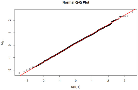
Figure 1.
Normal Q–Q plot of the modified [5] test under
.
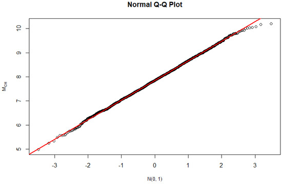
Figure 2.
Normal Q–Q plot of the modified [5] test under
.
5. Application to the Monthly Price Estimates of 36 Countries
The validity of the proposed
test procedure was ascertained using the monthly average estimates of the exchange rate and labor wage in agricultural markets for 36 countries. The aim here is to determine if there is a fractional cointegrating relationship between the United States Dollar (USD) exchange rate of each country and the labor wage. These 36 countries are classified as having similar agricultural economies according to the World Bank Development Economics Data Group (DECDG). The dataset was extracted from the World Bank Microdata Library. The dataset covers the period from January 2007 to June 2024 for 27 of the 36 countries, from January 2008 to June 2024 for Armenia, Guinea, and Myanmar, from January 2009 to June 2024 for Yemen, from January 2011 to June 2024 for the Republic of Congo and the Syrian Arab Republic, from January 2012 to June 2024 for Iraq and Lebanon, and from January 2017 to June 2024 for Libya.
Suppose we let
represent the USD exchange rate for
countries and
months, and
represents the labor wage. The underlying fractional cointegration model used to test the cointegration hypothesis is given by the following:
We estimated the fractional cointegration parameters
and
by applying a bandwidth parameter
, which corresponds to
for each individual country as well as for the combined panel of countries. The hypotheses tested to determine if the two variables exhibit fractional cointegration are as follows:
- and are not fractionally cointegrated if .
- and are fractionally cointegrated if . If the null hypothesis is rejected, it implies there is a long-run relationship between the exchange rate and labor wage such that if there is a deviation, it is only temporary.
Figure 3 shows the time plot of exchange rate
and labou = r wage
for Afghanistan, Armenia, Bangladesh, Burkina Faso, Burundi, Cameroon, Central African Republic, Chad, Democratic Republic of Congo, Republic of Congo, Gambia, and Guinea. The plots show that co-movement, which is an indication of the cointegration between the exchange rate and labor wage, is suspected across the 12 countries, and that it is more evident in Gambia.
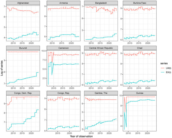
Figure 3.
Time plot of exchange rate
and labor wage
for Afghanistan, Armenia, Bangladesh, Burkina Faso, Burundi, Cameroon, Central African Republic, Chad, Democratic Republic of Congo, Republic of Congo, Gambia, and Guinea.
Figure 4 shows the time plot of exchange rate
and labor wage
for Guinea-Bisau, Haiti, Indonesia, Iraq, Kenya, Lao PDR, Lebanon, Liberia, Libya, Malawi, Mali, and Mauritania. The plots show that co-movement, which is an indication of the cointegration between the exchange rate and labor wage, is suspected across the 12 countries, and that it is more evident in Indonesia, Haiti, and Malawi.
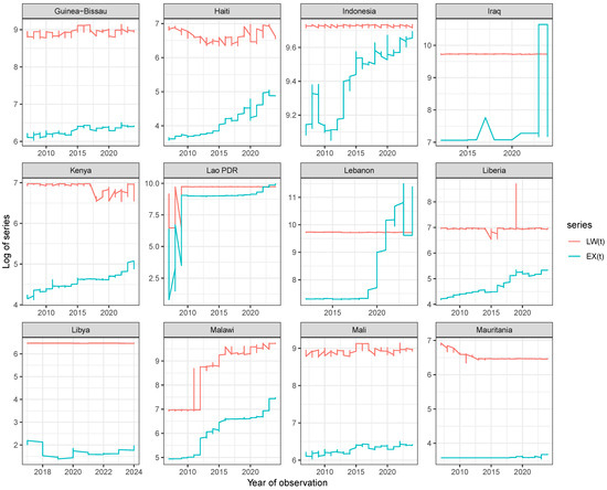
Figure 4.
Time plot of exchange rate
and labor wage
for Guinea-Bisau, Haiti, Indonesia, Iraq, Kenya, Lao PDR, Lebanon, Liberia, Libya, Malawi, Mali, and Mauritania.
Figure 5 shows the time plot of the exchange rate
and labor wage
for Mozambique, Myanmar, Niger, Nigeria, Philippines, Senegal, Somalia, South Sudan, Sri Lanka, Sudan, Syrian Arab Republic, and Yemen Republic. The plots show that co-movement, which is an indication of the cointegration between the exchange rate and labor wage, is suspected across the 12 countries, and that it is more evident in Nigeria, South Sudan, Yemen Rep., and the Syrian Arab Republic.
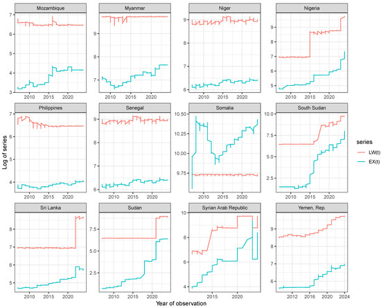
Figure 5.
Time plot of exchange rate
and labor wage
for Mozambique, Myanmar, Niger, Nigeria, Philippines, Senegal, Somalia, South Sudan, Sri Lanka, Sudan, Syrian Arab Republic, and Yemen Republic.
Table 3 presents the estimates of the fractional cointegration parameters
,
, and
, along with the proposed test statistic
and its corresponding p-value
for 36 countries and their panels. The p-value
refers to the probability that a standard normal random variable
takes a value greater than the absolute value of the test statistic
. Also, the results allow us to assess whether there is evidence of fractional cointegration between the exchange rate and labor wage in these countries. The fractional cointegration relationship is deemed significant if the test statistic
is sufficiently large and the p-value is below a conventional threshold (e.g., 0.05).
Table 3.
Fractional cointegration parameter
estimates and proposed test statistic and p-value
and
for 36 countries and their panels.
The majority of the countries exhibit significant fractional cointegration, as indicated by p-values less than 0.05. For example, Afghanistan (,
), Bangladesh (,
), and Burkina Faso (,
) all show strong evidence of fractional cointegration. This means that in these countries, the exchange rate and labor wage share a long-term equilibrium relationship, with deviations from this equilibrium expected to revert over time.
Conversely, ten countries do not exhibit significant fractional cointegration, as their p-values exceeded the 0.05 threshold. For instance, Cameroon (,
), the Democratic Republic of Congo (,
), and Libya (,
) did not show evidence of a fractional cointegrating relationship between their exchange rates and labor wages. For these countries, the lack of significant cointegration suggests that the two variables do not share a stable long-term relationship.
The panel data results, which aggregate the information across all 36 countries, indicate significant fractional cointegration (,
). This aggregated finding underscores the presence of a common long-term relationship between exchange rates and labor wages across the entire sample of countries, reinforcing the robustness of the individual country results, most especially for the 26 countries that showed evidence of long-run fractional cointegrating relationships.
6. Conclusions
In this paper, we proposed a modified Chen and Hurvich test for fixed-effect fractional cointegrated panels. An illustration is demonstrated using the simulation of several fractional cointegrated panels with varying real-valued orders spanning through weak stationarity to high non-stationarity. The test converges to a standard normal distribution under the null hypothesis and diverges under the alternative. The simulation results showed that the proposed test maintained the imposed Type I error rate with a considerably low type II error, which resulted in high power. Although the proposed test exhibited high power for nonstationary panels, the type I error is not significantly different from the original Chen and Hurvich test. Thus, there is still room for improvement in the validity of the test for series with
close to 1. Furthermore, the panel results from the monthly estimates from the 36 countries’ markets confirm the presence of a common fractional cointegration relationship across the entire sample. This highlights the generalizability and robustness of the findings, suggesting that the observed cointegration patterns are not isolated incidents but rather indicative of broader economic dynamics in agricultural markets.
In addition, the modified Chen and Hurvich test proposed in this study offers a practical tool for researchers and analysts working with fixed-effect fractional cointegrated panels, particularly in economic and financial datasets where traditional cointegration methods may fall short. By demonstrating robust performance across various simulations, the test provides a reliable approach for identifying cointegration relationships, even in nonstationary data. Its application to real-world data from 36 countries’ markets highlights its utility in understanding global economic dynamics, particularly in agriculture. The test’s ability to maintain high power while controlling type I error makes it valuable for accurately detecting long-term equilibrium relationships, which can inform better decision-making in policy, finance, and market analysis.
Furthermore, the outcomes of this research have significant social implications, particularly in understanding the interconnectedness of global agricultural markets. By confirming the presence of fractional cointegration relationships between exchange rates and labor wages across multiple countries, this study sheds light on the broader economic forces influencing wages and prices in agriculture. This insight is crucial for policymakers and stakeholders working to address global economic inequalities, stabilize agricultural markets, and ensure fair wages for workers. Moreover, the findings provide a more nuanced view of how global economic factors are linked, potentially contributing to more equitable and informed strategies for economic development and labor policy. Overall, this study underscores the importance of considering fractional cointegration in understanding the interplay between exchange rates and labor wages in the global agricultural economy.
Author Contributions
Conceptualization S.F.O. and O.R.O.; methodology, S.F.O.; software, S.F.O. and O.R.O.; validation, J.A. and A.A.A.; formal analysis, S.F.O. and O.R.O.; investigation, J.A. and A.A.A.; resources, S.F.O.; data curation, S.F.O.; writing—original draft preparation, S.F.O.; writing—review and editing, S.F.O., O.R.O., J.A. and A.A.A.; supervision, O.R.O. All authors have read and agreed to the published version of the manuscript.
Funding
This research received no external funding.
Data Availability Statement
The authors confirm that the data supporting the findings of this study are available within the article.
Conflicts of Interest
The authors declare no conflict of interest.
References
- Johansen, S.; Nielsen, M.Ø. Likelihood Inference for a Fractionally Cointegrated Vector Autoregressive Model. Econometrica 2012, 80, 2667–2732. [Google Scholar] [CrossRef][Green Version]
- Khodamoradi, T.; Salahi, M.; Najafi, A.R. A Note on CCMV Portfolio Optimization Model with Short Selling and Risk-neutral Interest Rate. Stat. Optim. Inf. Comput. 2020, 8, 740–748. [Google Scholar] [CrossRef]
- Mukhodobwane, R.M.; Sigauke, C.; Chagwiza, W.; Garira, W. Volatility Modelling of the BRICS Stock Markets. Stat. Optim. Inf. Comput. 2020, 8, 749–772. [Google Scholar] [CrossRef]
- Marmol, F.; Velasco, C. Consistent Testing of Cointegrating Relationships. Econometrica 2004, 72, 1809–1844. [Google Scholar] [CrossRef]
- Chen, W.W.; Hurvich, C.M. Semiparametric Estimation of Fractional Cointegrating Subspaces. Ann. Stat. 2006, 34, 2939–2979. [Google Scholar] [CrossRef][Green Version]
- Johansen, S. Representation of Cointegrated Autoregressive Processes with Application to Fractional Processes. Econom. Rev. 2008, 28, 121–145. [Google Scholar] [CrossRef]
- Robinson, P.M. Diagnostic Testing for Cointegration. J. Econom. 2008, 143, 206–225. [Google Scholar] [CrossRef][Green Version]
- Nielsen, M.Ø. Nonparametric Cointegration Analysis of Fractional Systems with Unknown Integration Orders. J. Econom. 2010, 155, 170–187. [Google Scholar] [CrossRef]
- Avarucci, M.; Velasco, C. A Wald Test for the Cointegration Rank in Nonstationary Fractional Systems. J. Econom. 2009, 151, 178–189. [Google Scholar] [CrossRef][Green Version]
- Łasak, K. Likelihood Based Testing for no Fractional Cointegration. J. Econom. 2010, 158, 67–77. [Google Scholar] [CrossRef]
- Johansen, S.; Nielsen, M.Ø. Nonstationary Cointegration in the Fractionally Cointegrated VAR Model. J. Time Ser. Anal. 2019, 40, 519–543. [Google Scholar] [CrossRef]
- Souza, I.V.M.; Reisen, V.A.; Franco, G.d.C.; Bondon, P. The Estimation and Testing of the Cointegration Order based on the Frequency Domain. J. Bus. Econ. Stat. 2018, 36, 695–704. [Google Scholar] [CrossRef]
- Leschinski, C.; Voges, M.; Sibbertsen, P. A Comparison of Semiparametric Tests for Fractional Cointegration. Stat. Pap. 2020, 62, 1997–2030. [Google Scholar] [CrossRef]
- Nielsen, M.Ø.; Shimotsu, K. Determining the Cointegrating Rank in Nonstationary Fractional Systems by the Exact Local Whittle Approach. J. Econom. 2007, 141, 574–596. [Google Scholar] [CrossRef]
- Robinson, P.M.; Yajima, Y. Determination of Cointegrating Rank in Fractional Systems. J. Econom. 2002, 106, 217–241. [Google Scholar] [CrossRef]
- Hualde, J.; Velasco, C. Distribution-Free Tests of Fractional Cointegration. Econom. Theory 2008, 24, 216–255. [Google Scholar] [CrossRef]
- Olaniran, S.F.; Ismail, M.T. A Comparative Analysis of Semiparametric Tests for Fractional Cointegration in Panel Data Models. Austrian J. Stat. 2022, 51, 96–119. [Google Scholar] [CrossRef]
- Engle, R.F.; Granger, C.W. Co-integration and Error correction: Representation, Estimation, and Testing. Econom. J. Econom. Soc. 1987, 55, 251–276. [Google Scholar] [CrossRef]
- Gujarati, D.N. Basic Econometrics, 4th ed.; McGraw-Hill: Singapore, 2003. [Google Scholar]
- Marinucci, D.; Robinson, P.M. Narrow-band analysis of nonstationary processes. Ann. Stat. 2001, 29, 947–986. [Google Scholar] [CrossRef]
- Robinson, P.M. Efficient tests of nonstationary hypotheses. J. Am. Stat. Assoc. 1994, 89, 1420–1437. [Google Scholar] [CrossRef]
- Chen, W.W.; Hurvich, C.M. Estimating fractional cointegration in the presence of polynomial trends. J. Econom. 2003, 117, 95–121. [Google Scholar] [CrossRef][Green Version]
- Ergemen, Y.E.; Velasco, C. Estimation of Fractionally Integrated Panels with Fixed Effects and Cross-section Dependence. J. Econom. 2017, 196, 248–258. [Google Scholar] [CrossRef]
- Robinson, P.M.; Velasco, C. Efficient inference on fractionally integrated panel data models with fixed effects. J. Econom. 2015, 185, 435–452. [Google Scholar] [CrossRef]
- Ergemen, Y.E. System estimation of panel data models under long-range dependence. J. Bus. Econ. Stat. 2019, 37, 13–26. [Google Scholar] [CrossRef]
- Zhang, R.; Robinson, P.; Yao, Q. Identifying cointegration by eigenanalysis. J. Am. Stat. Assoc. 2019, 114, 916–927. [Google Scholar] [CrossRef]
- Phillips, P.C. Optimal Inference in Cointegrated Systems. Econom. J. Econom. Soc. 1991, 59, 283–306. [Google Scholar] [CrossRef]
- Jamil, S.A.M.; Abdullah, M.A.A.; Kek, S.L.; Olaniran, O.R.; Amran, S.E. Simulation of Parametric Model towards the Fixed Covariate of Right Censored Lung Cancer Data. In Journal of Physics: Conference Series; IOP Publishing: Bristol, UK, 2017; Volume 890, p. 012172. [Google Scholar] [CrossRef]
- Olaniran, O.R.; Abdullah, M.A.A. Subset Selection in High-Dimensional Genomic Data using Hybrid Variational Bayes and Bootstrap priors. In Journal of Physics: Conference Series; IOP Publishing: Bristol, UK, 2020; Volume 1489, p. 012030. [Google Scholar] [CrossRef]
- Popoola, J.; Yahya, W.B.; Popoola, O.; Olaniran, O.R. Generalized Self-Similar First Order Autoregressive Generator (GSFO-ARG) for Internet Traffic. Stat. Optim. Inf. Comput. 2020, 8, 810–821. [Google Scholar] [CrossRef]
- Bala, N.M.; bin Safei, S. A Hybrid Harmony Search and Particle Swarm Optimization Algorithm (HSPSO) for Testing Non-functional Properties in Software System. Stat. Optim. Inf. Comput. 2021, 10, 968–982. [Google Scholar] [CrossRef]
- Olaniran, S.F.; Olaniran, O.R.; Allohibi, J.; Alharbi, A.A.; Ismail, M.T. A Generalized Residual-Based Test for Fractional Cointegration in Panel Data with Fixed Effects. Mathematics 2024, 12, 1172. [Google Scholar] [CrossRef]


Disclaimer/Publisher’s Note: The statements, opinions and data contained in all publications are solely those of the individual author(s) and contributor(s) and not of MDPI and/or the editor(s). MDPI and/or the editor(s) disclaim responsibility for any injury to people or property resulting from any ideas, methods, instructions or products referred to in the content. |
© 2024 by the authors. Licensee MDPI, Basel, Switzerland. This article is an open access article distributed under the terms and conditions of the Creative Commons Attribution (CC BY) license (https://creativecommons.org/licenses/by/4.0/).