Shallow-Water Wave Dynamics: Butterfly Waves, X-Waves, Multiple-Lump Waves, Rogue Waves, Stripe Soliton Interactions, Generalized Breathers, and Kuznetsov–Ma Breathers

Abstract

A nonlinear $(3+1)$-dimensional nonlinear Geng equation that can be utilized to explain the dynamics of shallow-water waves in fluids is given special attention. Various wave solutions are produced with the aid of the Hirota bilinear and Cole–Hopf transformation techniques. By selecting the appropriate polynomial function and implementing the distinct transformations in bilinear form, bright lump waves, dark lump waves, and rogue waves (RWs) are generated. A positive quadratic transformation and cosine function are combined in Hirota bilinear form to evaluate the RW solutions. Typically, RWs have crests that are noticeably higher than those of surrounding waves. These waves are also known as killer, freak, or monster waves. The lump periodic solutions (LPSs) are obtained using a combination of the cosine and positive quadratic functions. The lump-one stripe solutions are computed by using a mix of positive quadratic and exponential transformations to the governing equation. The lump two-stripe solutions are obtained by using a mix of positive quadratic and exponential transformations to the governing equation. The interactional solutions of lump, kink, and periodic wave solutions are obtained. Additionally, mixed solutions with butterfly waves, X-waves and lump waves are computed. The Ma breather (MB), Kuznetsov–Ma breather (KMB), and generalized breathers GBs are generated. Furthermore, solitary wave solution is obtained and a relation for energy of the wave via ansatz function technique.

1. Introduction

Unusually huge ocean waves, or rogue waves (RWs), can be extremely dangerous for ships and offshore building projects. These waves are also known as killer, freak, or monster waves. Compared to the waves nearby, these waves are substantially taller and more forceful. Because of their erratic behavior and sudden appearance, RWs pose a threat to marine life. RWs typically have crests that are substantially higher than those of nearby waves. They soar to a minimum of 100 feet, or 30 m, higher than the surrounding waves. Recently, RWs are modeled by using the nonlinear evolution equations (NLEEs). Many experts believe that nonlinear science is the best means to comprehend the fundamental concepts of physical laws and the complex nonlinearity phenomena. NLEEs explain a wide range of complex events and scientific fields, such as chemical reactions, biology, engineering, applied mathematics, and climate science. In order to understand the nuances of the system under analysis, one must solve NLEEs and find both their analytical and numerical solutions. The analytical solutions of these equations always advance our understanding of the natural world. Numerous efficient techniques have been developed to provide both analytical and numerical solutions for NLEEs. For instance, Bertoldi et al. worked on flexible mechanical metamaterials [1]. Holmes et al. worked on elasticity and stability of shape-shifting structures [2], Deng et al. studied the vector solitons in soft architected materials [3] and he also found the metamaterials with amplitude gaps for elastic solitons [4]. Raney et al. investigated the propagation of mechanical signals in soft media using stored elastic energy propagation of mechanical signals in soft media using stored elastic energy [5]. Edelman worked on stability of fractional logistic maps [6]. Shen et al. computed the complex-valued astigmatic cosine-Gaussian soliton solution of the nonlocal nonlinear Schrödinger equation and its transmission characteristics [7]. Song et al. worked on coherent superposition propagation of Laguerre–Gaussian and Hermite–Gaussian solitons [8]. Shen et al. investigated the periodic propagations for a complex valued hyperbolic cosine Gaussian solitons and breaathers in nonlinear media [9]. Yi et al. investigated High-order effect on the transmission of two optical solitons [10].

It is common knowledge that NLEEs can be used to explain the majority of phenomena that occur in mathematical physics and engineering domains. For instance, NLEEs are a good way to represent the processes of heat flow and wave propagation in physics. NLEEs control the majority of population models in ecology. NLEEs describe the dispersion of a chemically reactive substance [11]. Furthermore, NLEEs govern the majority of physical processes in the fields of quantum mechanics, fluid dynamics, electricity, plasma physics, shallow-water wave propagation, and many other models. For the purpose of explaining these natural occurrences in scientific and engineering models, NLEEs have emerged as a valuable tool. Hence, it becomes more important to be aware of all recent and traditional methods for solving NLEEs and the usage of these methods [12,13,14].

Waves that travel in water with a shallow depth in relation to their wavelength are known as shallow-water waves. For these waves, the shallow depth limits the vertical dimension of the water movement, causing a more noticeable horizontal motion. They are frequently found on continental shelves, in rivers, and along coastlines when the water depth is less than half the wavelength. Wave activity that wears away shorelines and changes coastal landform is largely caused by shallow-water waves [15,16]. Shallow ocean waves increase the load on structures such as seawalls, jetties, piers, and bridges. If structures are not sufficiently engineered to withstand the stresses exerted by these waves, particularly when they break, damage or even failure may result. Shallow-water waves can cause flooding in coastal locations, especially during storm surges, which can affect infrastructure, residential areas, and habitats. Wave energy is dispersed over a larger region when they break, which might occasionally aid in shoreline protection. But, over time, this can also result in the displacement of sediment and sand, changing the profiles of the shoreline and seabed [17,18,19]. Waves in shallow water frequently behave like solitons, particularly in certain situations where the wave holds its shape for extended periods of time. Particularly important in shallow-water scenarios, soliton waves are stable, solitary waves that result from a medium’s equilibrium between nonlinear and dispersive effects. They are especially helpful in characterizing the behavior of waves in coastal areas or canals where nonlinearity is substantial and depth is a bit uniform. Long-distance soliton energy has an effect on coastal structures when it arrives. In order to examine the energy and assess the effects of waves on harbors and coasts, it is necessary to integrate the kinetic and potential energy over the soliton profile.

We consider a (3 + 1)-dimensional nonlinear Geng equation as [20],

$$\begin{array}{c}\hfill 3u_{xz}-{\left(2u_t+u_{xxx}-2u{u}_x\right)}_y+2{\left(u_x{\partial }_x^{-1}{u}_y\right)}_x=0\end{array}$$

(1)

The Geng equation (Equation (1)) can be used to describe shallow-water wave dynamics. This model not only includes a classical Korteweg–de Vries (KdV) equation component but also contains nonlinear effect $u_x{\partial }_x^{-1}{u}_y$; ${\partial }_x^{-1}$ represents the integral with respect to x and $u_{xz}$ denotes the dispersion effects with x, y, z spatial components and t as the temporal component [20].

A few mathematicians have worked on (1); for example, Li et al. computed a hybrid soliton, molecules, and breather molecules of a (3 + 1)-Geng equation in shallow-water waves [20]. Ahmed et al. investigated homoclinic breathers and soliton propagations for the nonlinear (3 + 1)-Geng model [21]. Geng computed the algebraic–geometrical solutions of multi-dimensional nonlinear evolution equations [22]. Yin et al. investigated the exact solutions and diverse interaction phenomena via Bäcklund transformation to a (3 + 1)-dimensional nonlinear evolution equation [23]. Bai et al. found the soliton solutions to (3 + 1)-dimensional nonlinear equation by using a generalized method [24]. However, the goal of this work is to use the Hirota bilinear and Cole–Hopf transformation methods to extract distinct solutions for the specified model in the form of bright and dark lump waves, butterfly waves, X-waves, lump one-stripe soliton interaction, lump two-strip solitons interaction, LPS, RWs, and their interactions. We also find the MBs, KMBs, GBs, and SWs for the governing model. Furthermore, we develop a relation between the energy of the wave, impact of wave pressure on coastal structures, structural thickness, and safety factor.

The details of the rest of the work are as follows. In Section 2, we use the Hirota bilinear and Cole–Hopf transformation methods to compute the bright and dark lump waves for the given model. In Section 3, we study the bright lump with periodic waves. We compute the RW solutions via a positive quadratic transformation, and cosine functions in Section 4. We find the lump one-strip soliton interaction (L1SI) in Section 5 and lump two-strip soliton interaction (L2SI) in Section 6. We use the appropriate polynomial functions to generate the interaction between lump, periodic, and strip waves in Section 7. We use the appropriate polynomial functions to obtain the interaction between lump, RWs, and strip waves in Section 8. In Section 9, Section 10 and Section 11, we examine the MBs, KMBs, and GBs, respectively. Section 12 covers the symbolic computation using the ansatz function approach. In Section 13, we use the ansatz function approach to determine the SWs. Additionally, in Section 14 a relationship is established between wave energy, the effect of wave pressure on coastal structures. In Section 15 and Section 16 we will give the discussions and conclusions.

2. Bright and Dark Lump Waves

We first take the following Cole–Hopf transformation [12,13,17,18,19]:

$$\begin{array}{c}\hfill u=-3{\left(lnf\right)}_{xx},\end{array}$$

(2)

where $f=f(x,y,z,t)$ is an auxiliary function. With the usage of (2) in (1), we have the following bilinear form:

$$\begin{array}{c}\hfill \left\{\begin{array}{c}3f_{xy}{f}_{xx}+3\left(f_z-f_{xxy}\right)f_x-\left(2f_t+f_{xxx}\right)f_y+f\left(2f_{yt}-3f_{xz}+f_{xxxy}\right)=0,\hfill \\ or\hfill \\ \left(3D_x{D}_z-2D_y{D}_t-D_y{D}_x^3\right)\left(f.f\right)=0,\hfill \end{array}\right.\end{array}$$

(3)

where Hirota’s operator $D_x$ represents derivative with respect to x and $D_t$ represents derivative with respect to t, defined by $D_x^n{D}_t^m\left(f.f\right)={\left({\displaystyle \frac{\partial }{\partial x}}-{\displaystyle \frac{\partial }{\partial x^{\prime }}}\right)}^n{\left({\displaystyle \frac{\partial }{\partial t}}-{\displaystyle \frac{\partial }{\partial t^{\prime }}}\right)}^{m}f\left(x\right)f\left(x^{\prime }\right){|}_{x=x^{\prime },t=t^{\prime }}$.

Now, the function f in (3) can be assumed as [12,13]

$$f={\mho }_1^2+{\mho }_2^2+a_{11},$$

(4)

where ${\mho }_1=a_{1}x+a_{2}y+a_{3}z+a_{4}t+a_5$, ${\mho }_2=a_{6}x+a_{7}y+a_{8}z+a_{9}t+a_{10}$, $a_h(1\le h\le 11)$ are constants. Applying f to Equation (6) and resolving the coefficients of x, y, z, t and by using Mathematica 14.1 version, we get

Set I.

$$\begin{array}{c}\hfill \left\{\begin{array}{c}{a}_2={\displaystyle \frac{3\left(a_1{a}_3{a}_4+a_1{a}_8{a}_9+a_3{a}_6{a}_9-a_4{a}_6{a}_8\right)}{2\left(a_4^2+a_9^2\right)}},\hfill \\ a_7=-{\displaystyle \frac{3\left(a_1{a}_3{a}_4-a_1{a}_4{a}_8-a_3{a}_4{a}_6-a_8{a}_6{a}_9\right)}{2\left(a_4^2+a_9^2\right)}},\hfill \\ a_4=a_4,\hfill \\ a_5=a_5.\hfill \end{array}\right.\end{array}$$

(5)

Usage of (5) and (4) with (2) generates the solution

$$u_1={\displaystyle \frac{-6a_1{G}_1+6a_6{G}_2^2+3\left(2a_1^2+2a_6^2\right)\left(a_{11}+G_1^2\right)+3G_2^2}{{\left(\left(a_{11}+G_1^2\right)+G_2^2\right)}^2}},$$

(6)

where $G_1=\left(a_5+a_{4}t+a_{1}x+{\displaystyle \frac{3\left(a_1{a}_3{a}_4+a_1{a}_8{a}_9+a_3{a}_6{a}_9-a_4{a}_6{a}_8\right)y}{2\left(a_4^2+a_9^2\right)}}+a_{3}z\right)$,

$G_2=\left(a_5+a_{4}t+a_{1}x-{\displaystyle \frac{3\left(a_1{a}_3{a}_4-a_1{a}_4{a}_8-a_3{a}_4{a}_6-a_8{a}_6{a}_9\right)y}{2\left(a_4^2+a_9^2\right)}}+a_{3}z\right)$.

Set II. When

$$\begin{array}{c}\hfill \left\{\begin{array}{c}{a}_6=-{\displaystyle \frac{3a_1{a}_8-2a_2{a}_9}{3a_3}},\hfill \\ a_1=a_1,\hfill \\ a_7=-{\displaystyle \frac{3a_1{a}_3^2+3a_1{a}_8^2-2a_2{a}_8{a}_9}{2a_3{a}_9}},\hfill \\ a_4=a_4.\hfill \end{array}\right.\end{array}$$

(7)

By utilizing (7), (4), and (2),

$$u_2={\displaystyle \frac{-3{\left(2a_1\left(a_5+a_{4}t+a_{1}x+a_{2}y+a_{3}z\right)-\frac{2\left(3a_1{a}_8-2a_2{a}_9\right)G_3}{3a_3}\right)}^2+\left(2a_1^2+\frac{2\left(3a_1{a}_8-2a_2{a}_9\right)}{3a_3}\right)G_4}{{\left(a_{11}+{\left(a_5+a_{4}t+a_{1}x+a_{2}y+a_{3}z\right)}^2-\frac{2\left(3a_1{a}_8-2a_2{a}_9\right)G_3^2}{3a_3}\right)}^2}},$$

(8)

$$G_3=\left(a_{10}+a_{9}t-{\displaystyle \frac{\left(3a_1{a}_8-2a_2{a}_9\right)x}{3a_3}}-{\displaystyle \frac{\left(3a_1{a}_3^2+3a_1{a}_8^2-2a_2{a}_8{a}_9\right)y}{2a_3{a}_9}}+a_{8}z\right),$$

$$G_4={\left(a_{11}+{\left(a_5+a_{4}t+a_{1}x+a_{2}y+a_{3}z\right)}^2+a_{10}+a_{9}t-{\displaystyle \frac{\left(3a_1{a}_8-2a_2{a}_9\right)x}{3a_3}}-{\displaystyle \frac{\left(3a_1{a}_3^2+3a_1{a}_8^2-2a_2{a}_8{a}_9\right)y}{2a_3{a}_9}}+a_{8}z\right)}^2.$$

3. Bright–Dark Lump with Periodic Waves (BLPs)

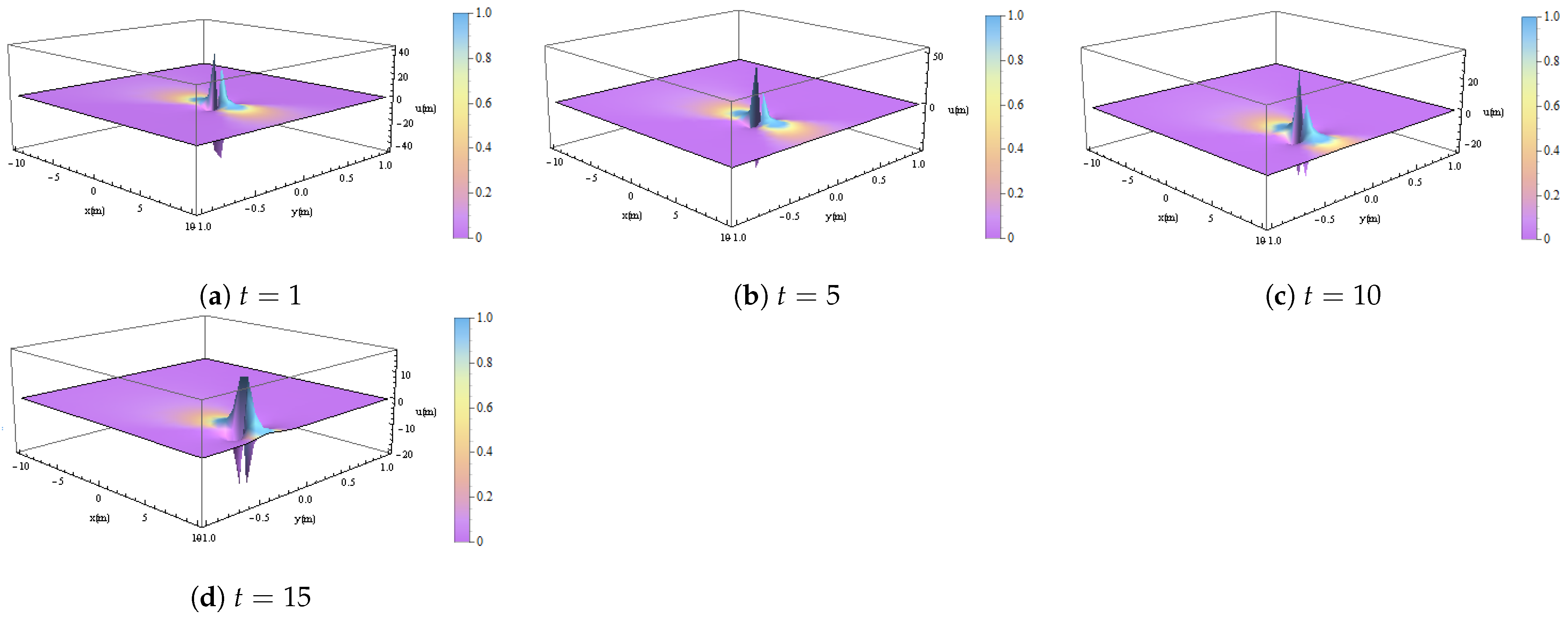
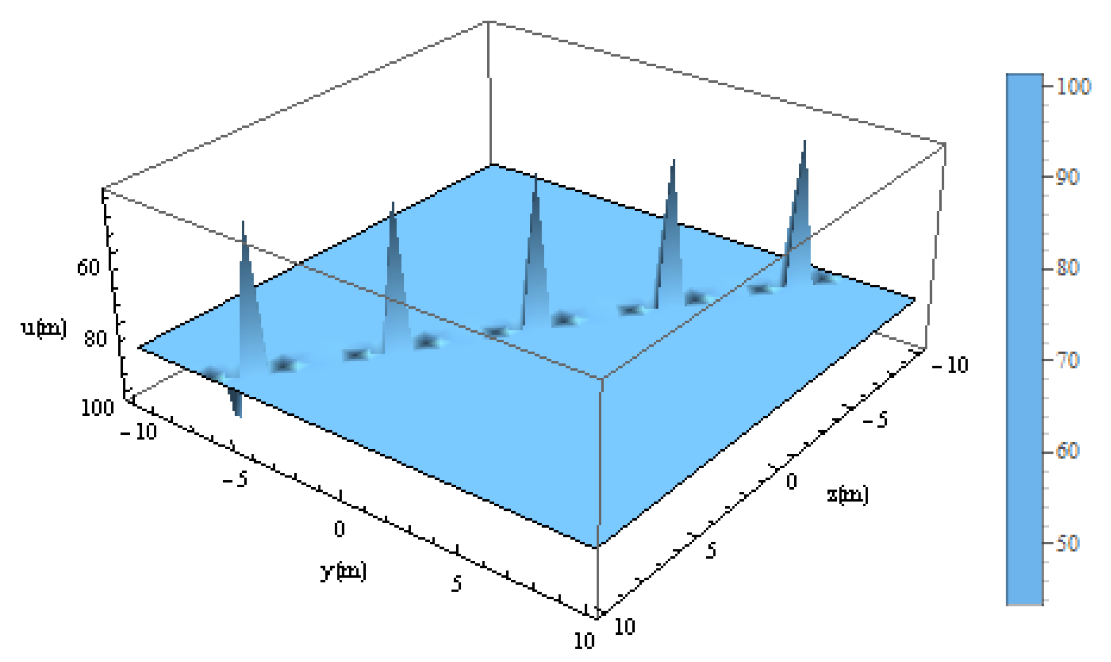
We choose f as [12,13]

$$f={\mho }_1^2+{\mho }_2^2+a_{11}+b_{1}cos(k_{1}x+k_{2}y+k_{3}z+k_{4}t),$$

(9)

where ${\mho }_1=a_{1}x+a_{2}y+a_{3}z+a_{4}t+a_5$, ${\mho }_2=a_{6}x+a_{7}y+a_{8}z+a_{9}t+a_{10}$, $a_k(1\le k\le 11)$, $k_i(1\le k\le 4)$, and $b_1$ are constants.

Utilising equations drawn from the coefficients of cos, x, y, z, and t, as well as (9), (3) and by using Mathematica 14.1 version,

Set I.

$$\begin{array}{c}\hfill \left\{\begin{array}{c}{k}_2=-{\displaystyle \frac{k_1\left(a_7{k}_1^3-2a_7{k}_4+3a_8{k}_1\right)}{2\left(a_8{k}_1^3+a_6{k}_4-a_9{k}_1\right)}},\hfill \\ a_2={\displaystyle \frac{a_4{a}_7}{a_9}}{k}_3=-{\displaystyle \frac{\left(a_7{k}_1^3-2a_7{k}_4+3a_8{k}_1\right)\left(k_1^3-2k_4\right)}{6\left(a_8{k}_1^3+a_6{k}_4-a_9{k}_1\right)}},\hfill \\ a_2=0,\hfill \\ a_1=a_1,a_4=0.\hfill \end{array}\right.\end{array}$$

(10)

By using (10), (9), and (2),

$$u_3=-3\left({\displaystyle \frac{a_{11}+{\left(a_5+a_{1}x+a_{3}z\right)}^2+{\left(a_{10}+a_{9}t+a_{7}y+a_{8}z\right)}^2+N_1\left(2a_1^2+2a_6^2-N_1\right)-N_2}{a_{11}+{\left(a_5+a_{1}x+a_{3}z\right)}^2+{\left(a_{10}+a_{9}x+a_{7}y+a_{8}z\right)}^2-N_3}}\right),$$

(11)

where $N_1=b_{1}cos\left(k_{4}t+k_{1}x-{\displaystyle \frac{k_1\left(a_7{k}_1^3-2a_7{k}_4+3a_8{k}_1\right)y}{2\left(a_8{k}_1^3+a_6{k}_4-a_9{k}_1\right)}}+-{\displaystyle \frac{\left(a_7{k}_1^3-2a_7{k}_4+3a_8{k}_1\right)\left(k_1^3-2k_4\right)z}{6\left(a_8{k}_1^3+a_6{k}_4-a_9{k}_1\right)}}\right)$,

$N_2=2a_1^2+2a_6^2-b_1{k}_1^{2}cos\left(k_{4}t+k_{1}x-{\displaystyle \frac{k_1\left(a_7{k}_1^3-2a_7{k}_4+3a_8{k}_1\right)y}{2\left(a_8{k}_1^3+a_6{k}_4-a_9{k}_1\right)}}+-{\displaystyle \frac{\left(a_7{k}_1^3-2a_7{k}_4+3a_8{k}_1\right)\left(k_1^3-2k_4\right)z}{6\left(a_8{k}_1^3+a_6{k}_4-a_9{k}_1\right)}}\right)$,

$N_3=S_5-b_1{k}_{1}sin{\left(k_{4}t+k_{1}x-{\displaystyle \frac{k_1\left(a_7{k}_1^3-2a_7{k}_4+3a_8{k}_1\right)y}{2\left(a_8{k}_1^3+a_6{k}_4-a_9{k}_1\right)}}+-{\displaystyle \frac{\left(a_7{k}_1^3-2a_7{k}_4+3a_8{k}_1\right)\left(k_1^3-2k_4\right)z}{6\left(a_8{k}_1^3+a_6{k}_4-a_9{k}_1\right)}}\right)}^2$,

$S_5=2a_1\left(a_5+a_{1}x+a_{3}z\right)+2a_6\left(a_{10}+a_{9}t+a_{7}y+a_{8}z\right)$.

Set II.

$$\begin{array}{c}\hfill \left\{\begin{array}{c}{a}_1={\displaystyle \frac{k_2\left(k_1^3+2k_4\right)}{3a_4{a}_9{k}_3}},\hfill \\ a_2={\displaystyle \frac{a_4{a}_7}{a_9}},\hfill \\ a_4=a_4,\hfill \\ a_5=a_5.\hfill \end{array}\right.\end{array}$$

(12)

By using (12), (9), and (2),

$$u_4=-3\left({\displaystyle \frac{\left(a_{11}+{\left(a_5+a_{4}t+\frac{k_2\left(k_1^3+2k_4\right)x}{3a_4{a}_9{k}_3}+\frac{a_4{a}_{7}y}{a_9}+a_{3}z\right)}^2+S_1\right)S_2-S_3}{a_{11}+{\left(a_5+a_{4}t+\frac{k_2\left(k_1^3+2k_4\right)x}{3a_4{a}_9{k}_3}+\frac{a_4{a}_{7}y}{a_9}+a_{3}z\right)}^2+{\left(a_{10}+a_{9}t+a_{6}x+a_{7}y+a_{8}z\right)}^2+S_4}}\right),$$

(13)

where $S_1={\left(a_{10}+a_{9}t+a_{6}x+a_{7}y+a_{8}z\right)}^2+b_{1}cos\left(k_{4}t+k_{1}x+k_{2}y+k_{3}z\right)$,

$S_2=\left(2a_6^2+{\displaystyle \frac{2k_2^2{\left(k_1^3+2k_4\right)}^2}{{\left(3a_4{a}_9{k}_3\right)}^2}}-b_{1}cos\left(k_{4}t+k_{1}x+k_{2}y+k_{3}z\right)\right)$,

$S_2=\left(2a_6^2+{\displaystyle \frac{2k_2^2{\left(k_1^3+2k_4\right)}^2}{{\left(3a_4{a}_9{k}_3\right)}^2}}-b_{1}cos\left(k_{4}t+k_{1}x+k_{2}y+k_{3}z\right)\right)$,

$\begin{array}{c}{S}_3=(a_{11}+{\left(a_5+a_{4}t+{\displaystyle \frac{k_2\left(k_1^3+2k_4\right)x}{3a_4{a}_9{k}_3}}+{\displaystyle \frac{a_4{a}_{7}y}{a_9}}+a_{3}z\right)}^2+{\left(a_{10}+a_{9}t+a_{6}x+a_{7}y+a_{8}z\right)}^2\hfill \\ +b_{1}cos\left(k_{4}t+k_{1}x+k_{2}y+k_{3}z\right)),\hfill \end{array}$

$S_4=b_{1}cos{\left(k_{4}t+k_{1}x+k_{2}y+k_{3}z\right)}^2$.

4. Rogue Wave (RW)

We choose f as [12,13]

$$f={\mho }_1^2+{\mho }_2^2+a_{11}+b_{1}cosh(k_{1}x+k_{2}y+k_{3}z+k_{4}t),$$

(14)

where ${\mho }_1=a_{1}x+a_{2}y+a_{3}z+a_{4}t+a_5$, ${\mho }_2=a_{6}x+a_{7}y+a_{8}z+a_{9}t+a_{10}$, $a_k(1\le k\le 11)$, $k_i(1\le k\le 4)$, and $b_1$ are constants. Equations taken from the coefficients of sinh, cosh, x, y, z, and t can be solved using (14) and (3):

Set I.

$$\begin{array}{c}\hfill \left\{\begin{array}{c}{a}_2=-{\displaystyle \frac{\left(a_7{k}_1^3-2a_7{k}_4+3a_8{k}_1\right)}{a_8{k}_1^3-2k_4}},\hfill \\ a_4={\displaystyle \frac{a_9\left(a_7{k}_1^3-2a_7{k}_4+3a_8{k}_1\right)}{a_8{k}_1^3-2k_4}},\hfill \\ a_1=a_1,\hfill \\ a_5=a_5.\hfill \end{array}\right.\end{array}$$

(15)

By using (15), (14), and (2),

$$u_5=-3\left({\displaystyle \frac{a_{11}+\left({\left(a_5+\frac{a_9\left(a_7{k}_1^3-2a_7{k}_4+3a_8{k}_1\right)t}{a_7\left(k_1^3-2k_4\right)}+a_{1}x+\frac{\left(a_7{k}_1^3-2a_7{k}_4+3a_8{k}_1\right)y}{a_8{k}_1^3-2k_4}+a_{3}z\right)}^2+M_1\right)M_2^2}{a_{11}+{\left(a_5+\frac{a_9\left(a_7{k}_1^3-2a_7{k}_4+3a_8{k}_1\right)t}{a_7\left(k_1^3-2k_4\right)}+a_{1}x+\frac{\left(a_7{k}_1^3-2a_7{k}_4+3a_8{k}_1\right)y}{a_8{k}_1^3-2k_4}+M_1\right)}^2}}\right),$$

(16)

where $M_1={\left(a_{10}+a_{9}t+a_{6}x+a_{7}y+a_{8}z\right)}^2+b_{1}cos\left(k_{4}t+k_{1}x+k_{2}y+k_{3}z\right)$,

$M_2=2a_1^2+2a_6^2-b_1{k}_1^{2}cos\left(k_{4}t+k_{1}x+k_{2}y+k_{3}z\right)$ and

$\begin{array}{c}{M}_3=2a_1(a_5+{\displaystyle \frac{a_9\left(a_7{k}_1^3-2a_7{k}_4+3a_8{k}_1\right)t}{a_7\left(k_1^3-2k_4\right)}}+a_{1}x+{\displaystyle \frac{\left(a_7{k}_1^3-2a_7{k}_4+3a_8{k}_1\right)y}{a_8{k}_1^3-2k_4}}+a_{3}z)+\hfill \\ 2a_6\left(a_{10}+a_{9}t+a_{6}x+a_{7}y+a_{8}z\right)-b_1{k}_{1}sin\left(k_{4}t+k_{1}x+k_{2}y+k_{3}z\right)\hfill \end{array}$,

Set II.

$$\begin{array}{c}\hfill \left\{\begin{array}{c}{a}_4={\displaystyle \frac{{\left(-k_4\right)}^{\frac{1}{3}}{a}_8{a}_9}{{\left(-k_4\right)}^{\frac{1}{3}}{a}_8-a_7{k}_4}},\hfill \\ k_2={\displaystyle \frac{3{\left(-k_4\right)}^{\frac{1}{3}}{a}_8-a_7{k}_4}{a_9}},\hfill \\ k_3={\displaystyle \frac{3k_4{\left(-k_4\right)}^{\frac{2}{3}}{a}_7+a_8}{2a_9}},\hfill \\ a_2=0,k_1={\left(-k_4\right)}^{{\displaystyle \frac{1}{3}}}.\hfill \end{array}\right.\end{array}$$

(17)

By using (17), (14), and (2),

$$u_6={\displaystyle \frac{\left(-3\left(a_{11}+{\left(a_5+\frac{{\left(-k_4\right)}^{\frac{1}{3}}{a}_8{a}_{9}t}{{\left(-k_4\right)}^{\frac{1}{3}}{a}_8-a_7{k}_4}+a_{1}x+a_{3}z\right)}^2+{\left(a_{10}+a_{9}x+a_{7}y+a_{8}z\right)}^2+I_1\right)I_2-I_3\right)}{{\left(a_{11}+{\left(a_5+\frac{{\left(-k_4\right)}^{\frac{1}{3}}{a}_8{a}_{9}t}{{\left(-k_4\right)}^{\frac{1}{3}}{a}_8-a_7{k}_4}+a_{1}x+a_{3}z\right)}^2+{\left(a_{10}+a_{9}x+a_{7}y+a_{8}z\right)}^2+{I_1}^2\right)}^2}},$$

(18)

where $I_1=b_{1}cos\left(k_{4}t+{\left(-k_4\right)}^{{\displaystyle \frac{1}{3}}}x+{\displaystyle \frac{\left(3{\left(-k_4\right)}^{\frac{1}{3}}{a}_8-a_7{k}_4\right)y}{2a_9}}+{\displaystyle \frac{3\left(k_4{\left(-k_4\right)}^{\frac{2}{3}}{a}_7+a_8\right)z}{2a_9}}\right),$

$I_2=2a_1^2+2a_6^2-b_{1}cos\left(k_{4}t+{\left(-k_4\right)}^{{\displaystyle \frac{1}{3}}}x+{\displaystyle \frac{\left(3{\left(-k_4\right)}^{\frac{1}{3}}{a}_8-a_7{k}_4\right)y}{2a_9}}+{\displaystyle \frac{3\left(k_4{\left(-k_4\right)}^{\frac{2}{3}}{a}_7+a_8\right)z}{2a_9}}\right)$,

$I_3=2a_1\left(a_5+{\displaystyle \frac{{\left(-k_4\right)}^{\frac{1}{3}}{a}_8{a}_{9}t}{{\left(-k_4\right)}^{\frac{1}{3}}{a}_8-a_7{k}_4}}+a_{1}x+a_{3}z\right)+2a_6\left(a_{10}+a_{9}x+a_{7}y+a_{8}z\right)-S_6$ and

$S_6=-b_1{\left(-k_4\right)}^{{\displaystyle \frac{1}{3}}}sin{\left(k_{4}t+{\left(-k_4\right)}^{{\displaystyle \frac{1}{3}}}x+{\displaystyle \frac{\left(3{\left(-k_4\right)}^{\frac{1}{3}}{a}_8-a_7{k}_4\right)y}{2a_9}}+{\displaystyle \frac{3\left(k_4{\left(-k_4\right)}^{\frac{2}{3}}{a}_7+a_8\right)z}{2a_9}}\right)}^2$.

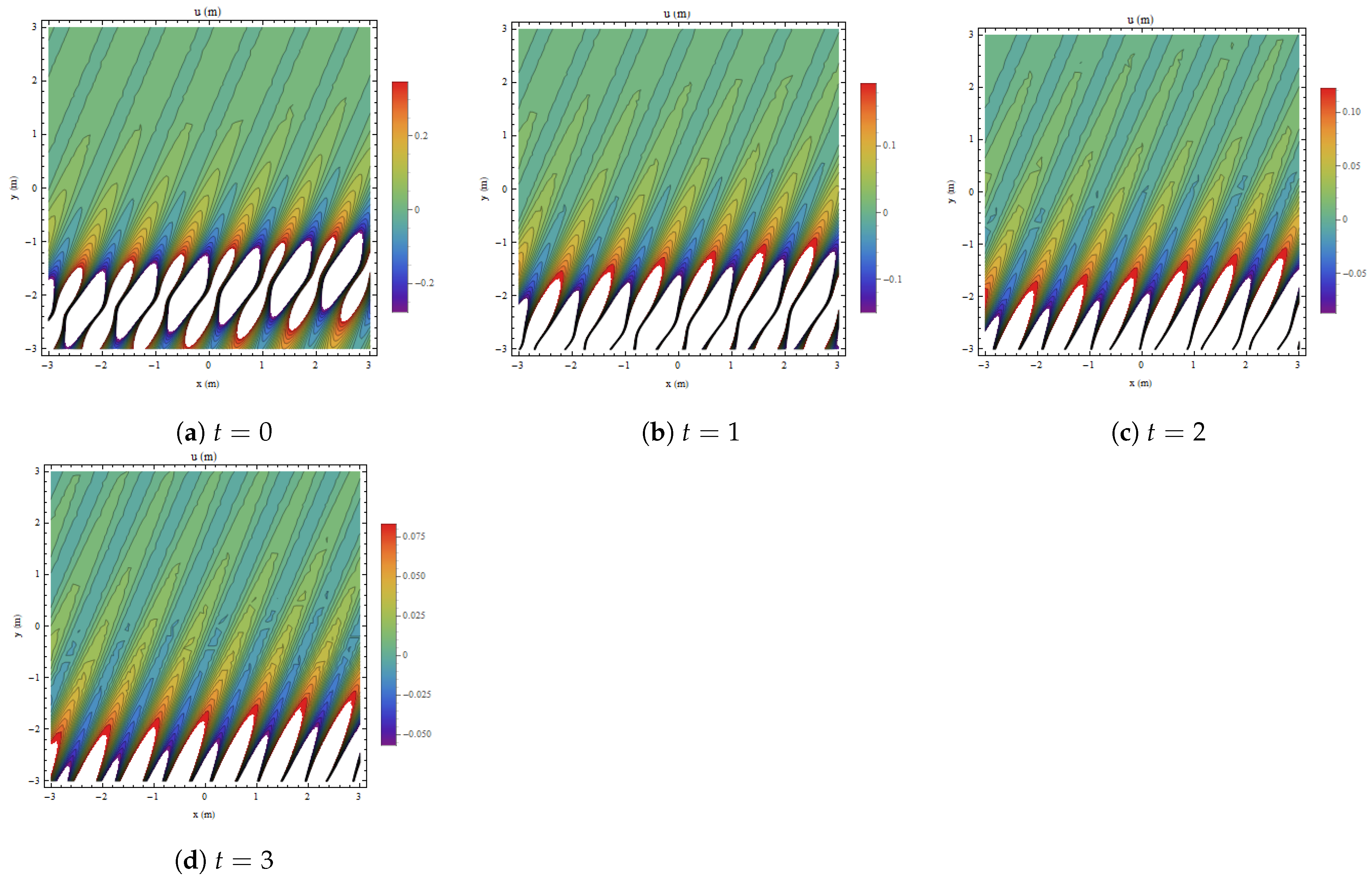
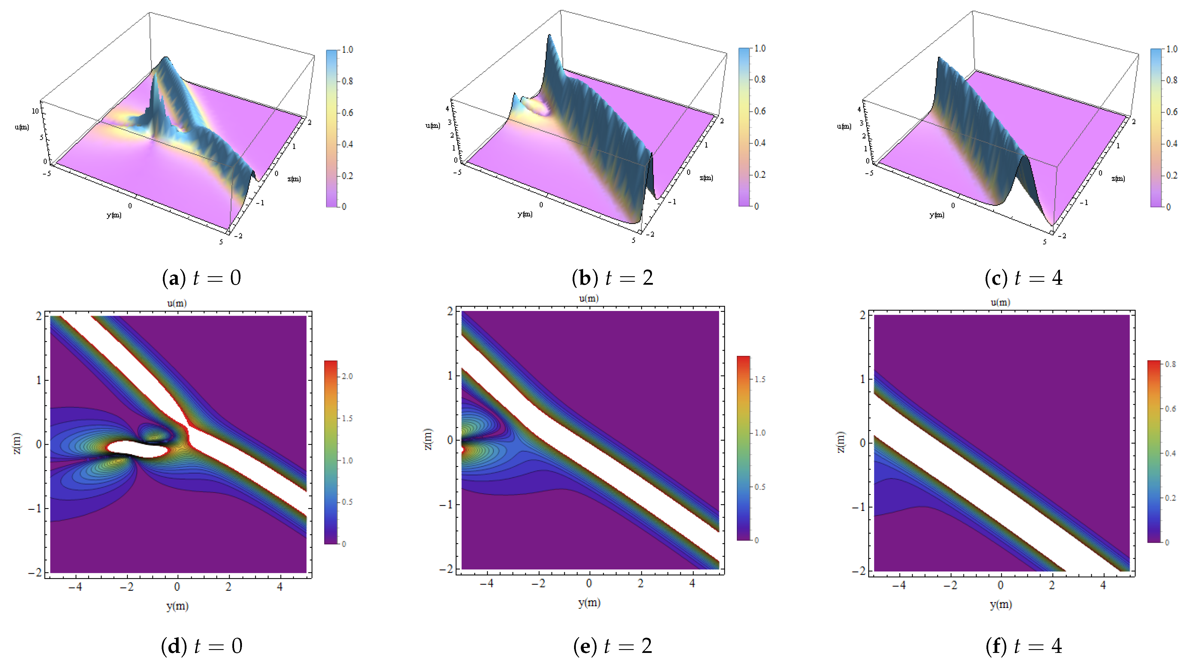
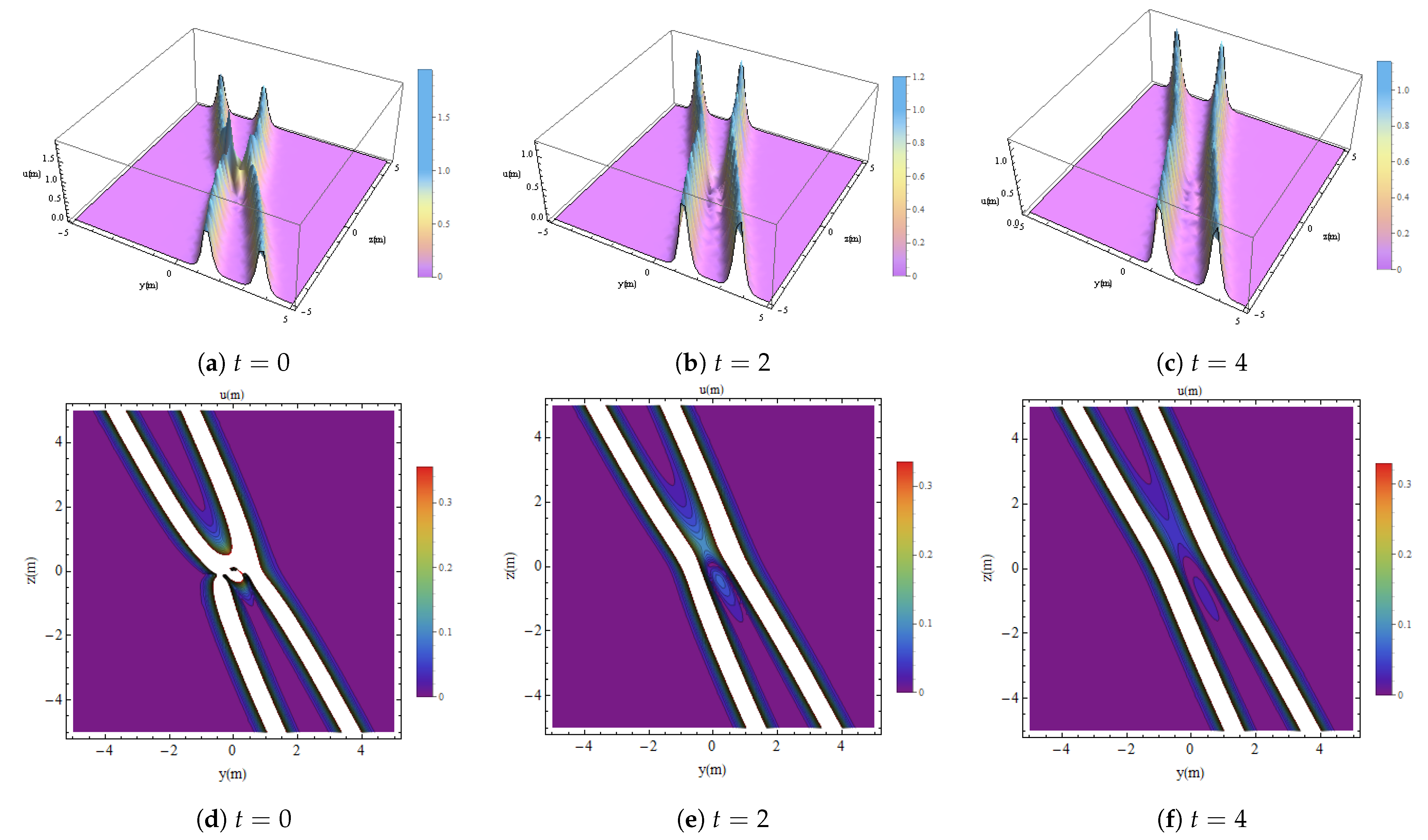
5. Lump One-Strip Soliton Interaction (L1SI)

We use f such that [12,13]

$$f={\mho }_1^2+{\mho }_2^2+a_{11}+b_1{e}^{k_{1}x+k_{2}y+k_{3}z+k_{4}t},$$

(19)

where ${\mho }_1=a_{1}x+a_{2}y+a_{3}z+a_{4}t+a_5$, ${\mho }_2=a_{6}x+a_{7}y+a_{8}z+a_{9}t+a_{10}$, $a_k(1\le k\le 11)$ are constants. By using (19) and (3) and collecting equations from the coefficients of $exp$, x, y, z, t and using Mathematica 14.1 version we get,

Set I.

$$\begin{array}{c}\hfill \left\{\begin{array}{c}{k}_3={\displaystyle \frac{k_2\left(k_1^2+2k_4\right)}{3k_1}},\hfill \\ a_8=a_8,\hfill \\ a_4=a_4,\hfill \\ a_5=a_5.\hfill \end{array}\right.\end{array}$$

(20)

By using (20), (19), and (2),

$$u_7=-3\left({\displaystyle \frac{{\left(b_1{e}^{k_{4}t+k_{1}x+k_{2}y}+\frac{k_2\left(k_1^2+2k_4\right)z}{3k_1}{k}_1+L_1\right)}^2+\left(2a_1^2+2a_6^2+b_1{e}^{k_{4}t+k_{1}x+k_{2}y}+\frac{k_2\left(k_1^2+2k_4\right)z}{3k_1}{k}_1^2\right)L_2}{{\left(a_{11}+b_1{e}^{k_{5}x+k_{6}y+k_{7}y+k_{8}z}+\frac{k_2\left(k_1^2+2k_4\right)z}{3k_1}+{\left(a_{54}+a_{4}x+a_{7}y+a_{8}z\right)}^2+{\left(a_{10}+a_{9}x+a_{7}y+a_{8}z\right)}^2\right)}^2}}\right),$$

(21)

where $L_1=2a_1\left(a_5+a_{4}t+a_{1}x+a_{2}y+a_{3}z\right)+2a_6\left(a_{10}+a_{9}t+a_{7}y+a_{8}z\right)$,

$L_2=(a_{11}+b_1{e}^{k_{4}t+k_{1}x+k_{2}y}+{\displaystyle \frac{k_2\left(k_1^2+2k_4\right)z}{3k_1}}+{\left(a_5+a_{4}t+a_{1}x+a_{2}y+a_{3}z\right)}^2+$${\left(a_{10}+a_{9}t+a_{7}y+a_{8}z\right)}^2)$.

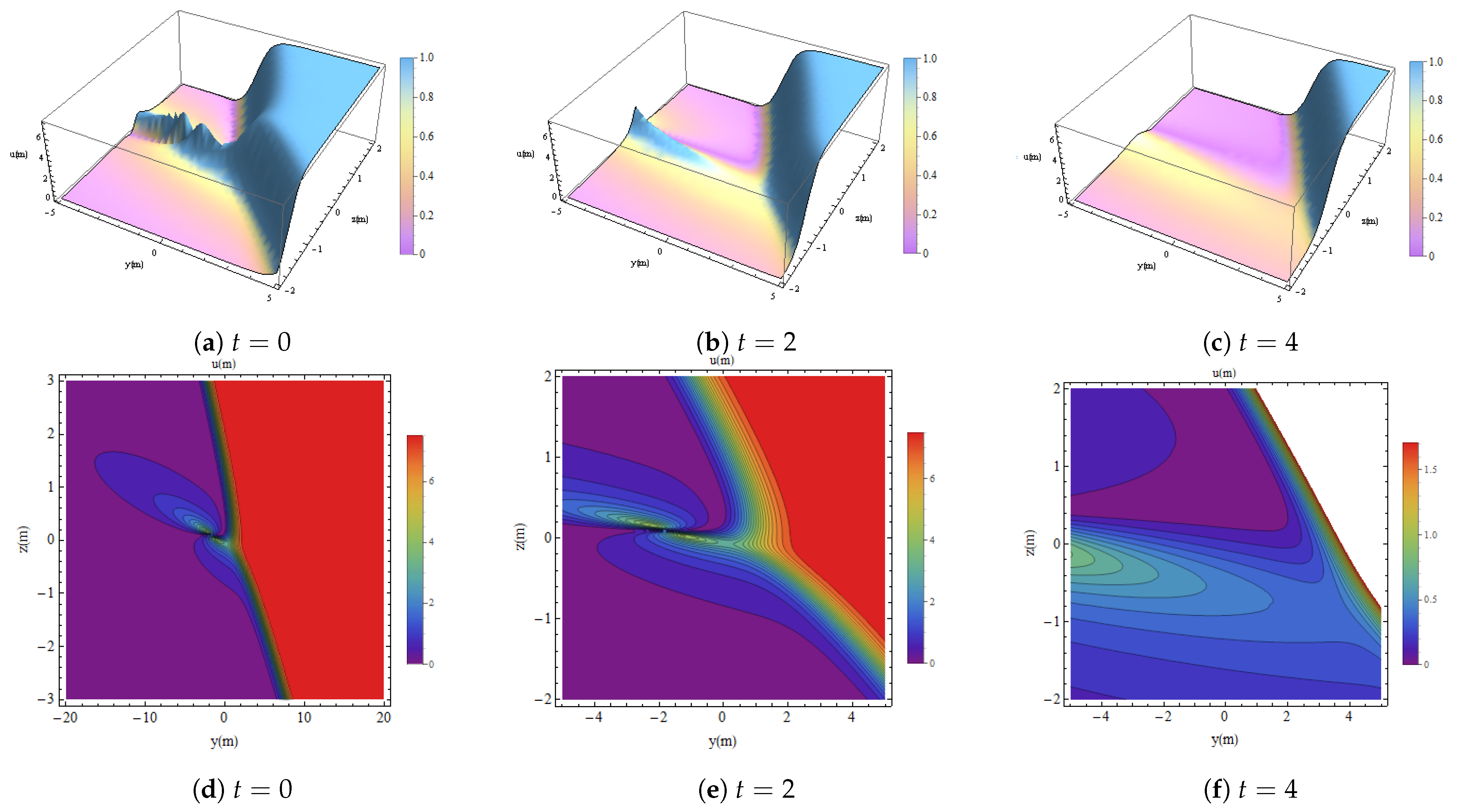
6. Lump Two-Strip Soliton Interaction (L2SI)

We employ the transformation in Equation (5), which is provided as [12,13]

$$f={\mho }_1^2+{\mho }_2^2+a_{11}+b_1{e}^{k_{1}x+k_{2}y+k_{3}z+k_{4}t}+b_2{e}^{-k_{1}x+k_{2}y+k_{3}z+k_{4}t},$$

(22)

where ${\mho }_1=a_{1}x+a_{2}y+a_{3}z+a_{4}t+a_5$, ${\mho }_2=a_{6}x+a_{7}y+a_{8}z+a_{9}t+a_{10}$, $k_i(1\le i\le 11)$$a_j(1\le j\le 11)$ are constants. By using (22) and (3) and collecting equations from the coefficients of $exp$, x, y, z, t and using Mathematica 14.1 version we get,

Set I.

$$\begin{array}{c}\hfill \left\{\begin{array}{c}{a}_8=-{\displaystyle \frac{a_1^2{k}_1{k}_2-a_{10}^2{k}_1{k}_3-a_5^2{k}_1{k}_3+a_6^2{k}_1{k}_2+a_1{a}_5{k}_3+a_{10}{a}_6{k}_3+a_3{a}_5{k}_1-a_1{a}_3}{a_{10}{k}_1-a_6}},\hfill \\ k_4=-{\displaystyle \frac{k_1\left(k_1^2{k}_2-3k_3\right)}{2k_2}},\hfill \\ a_7=k_2{a}_{10}.\hfill \end{array}\right.\end{array}$$

(23)

Using (23), (22), and (3),

$$u_8={\displaystyle \frac{-3\left(b_1{k}_1{e}^{-\frac{k_1\left(k_1^2{k}_2-3k_3\right)t}{2k_2}+k_{1}x+k_{2}y+k_{3}z}+b_2{k}_1{e}^{-\frac{k_1\left(k_1^2{k}_2-3k_3\right)t}{2k_2}+k_{1}x+k_{2}y+k_{3}z}+2a_1\left(a_5+a_{4}t+a_{1}x+a_{2}y+a_{3}z\right)+2a_6{L}_3\right)}{\left(a_{11}+b_1{e}^{-\frac{k_1\left(k_1^2{k}_2-3k_3\right)t}{2k_2}+k_{1}x+k_{2}y+k_{3}z}+b_2{e}^{-\frac{k_1\left(k_1^2{k}_2-3k_3\right)t}{2k_2}+k_{1}x+k_{2}y+k_{3}z}+{\left(a_5+a_{4}t+a_{1}x+a_{2}y+a_{3}z\right)}^2+L_3^2\right)}},$$

(24)

where $L_3$ is equal to the following:

$$L_3=\left(-{\displaystyle \frac{\left(a_1^2{k}_1{k}_2-a_{10}^2{k}_1{k}_3-a_5^2{k}_1{k}_3+a_6^2{k}_1{k}_2+a_1{a}_5{k}_3+a_{10}{a}_6{k}_3+a_3{a}_5{k}_1-a_1{a}_3\right)z}{a_{10}{k}_1-a_6}}+a_{10}+a_{9}t+a_{6}x+a_{10}{k}_{2}y\right).$$

(25)

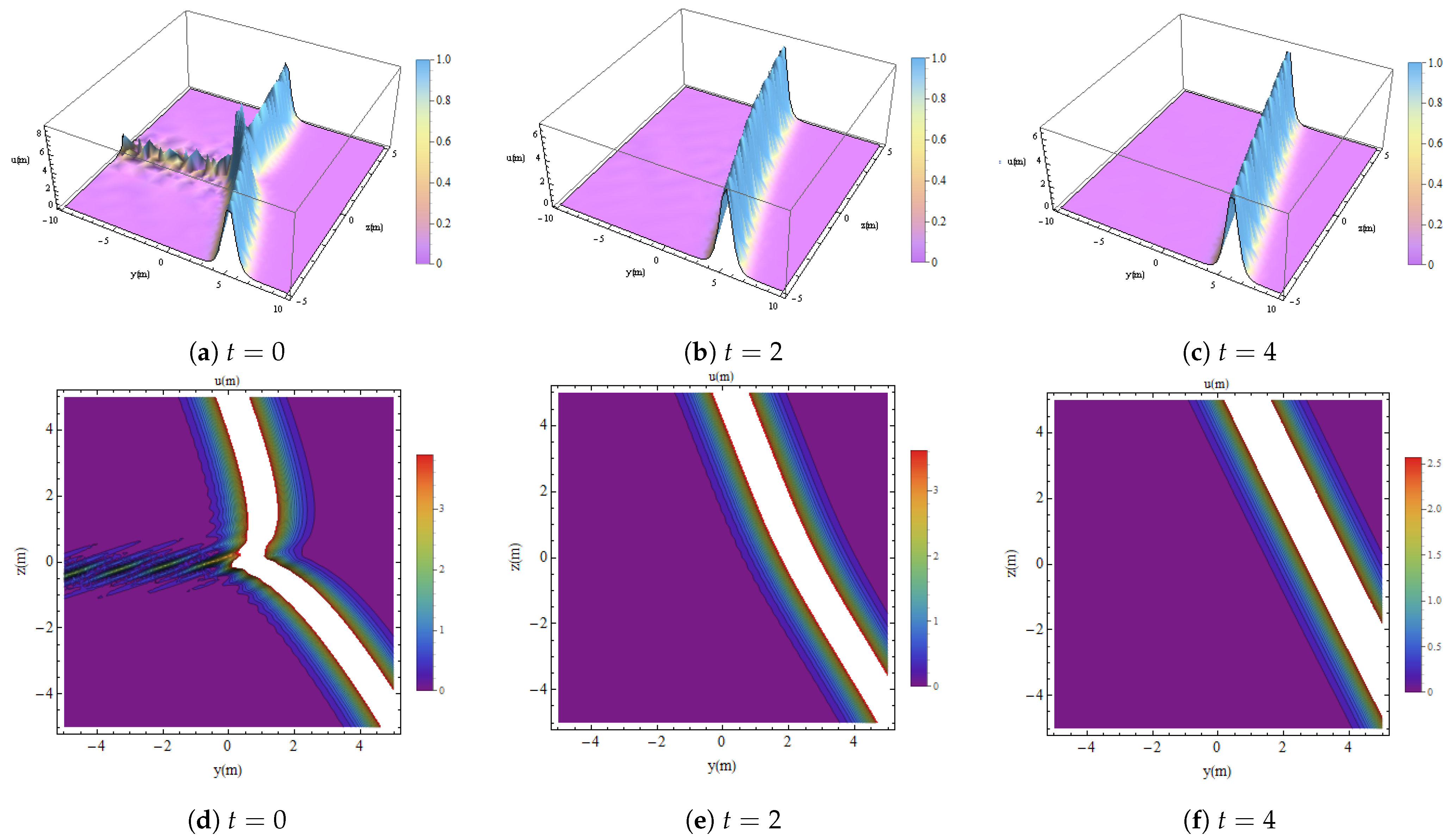
7. Interaction Between Lump, Periodic, and Strip Waves

We use f such that [12,13]

$$f={\mho }_1^2+{\mho }_2^2+a_{11}+b_{1}cos(k_{1}x+k_{2}y+k_{3}z+k_{4}t)+b_2{e}^{k_{1}x+k_{2}y+k_{3}z+k_{4}t},$$

(26)

where ${\mho }_1=a_{1}x+a_{2}y+a_{3}z+a_{4}t+a_5$, ${\mho }_2=a_{6}x+a_{7}y+a_{8}z+a_{9}t+a_{10}$, $a_k(1\le k\le 11)$ are constants. Equations derived from the coefficients of $exp$, cos $x,yz$, and t are solved using (26) and (3).

Set I.

$$\begin{array}{c}\hfill \left\{\begin{array}{c}{k}_3={\displaystyle \frac{k_1^2{k}_6+k_1^2{k}_7+2k_1{k}_2{k}_5-k_5^2{k}_6-k_5^2{k}_7+3k_8}{2k_1{k}_5}},\hfill \\ k_4={\displaystyle \frac{k_1^4{k}_6+k_1^2{k}_7+2k_1^2{k}_5^2{k}_7+k_5^4{k}_6+k_5^4{k}_7+3k_1^2{k}_8-3k_5^2{k}_8}{6k_1{k}_5}},\hfill \\ a_1={\displaystyle \frac{a_3{a}_6}{a_8}},a_2={\displaystyle \frac{a_3{a}_7}{a_8}},\hfill \\ a_8={\displaystyle \frac{a_8{a}_6}{a_3}}.\hfill \end{array}\right.\end{array}$$

(27)

By using (27), (26), and (2),

$$u_9=-3\left({\displaystyle \frac{a_{11}+b_2{e}^{k_{5}x+k_{6}y+k_{7}y+k_{8}z}+{\left(a_5-\frac{a_3{a}_{6}x}{a_8}+\frac{a_3{a}_{7}y}{a_8}+\frac{a_8{a}_{9}t}{a_3}+a_{3}z\right)}^2+{\left(a_{10}+a_{9}x+a_{7}y+a_{8}z\right)}^2+b_{1}cos\left(W_1\right)+W_2}{a_{11}+b_2{e}^{k_{5}x+k_{6}y+k_{7}y+k_{8}z}+{\left(a_5-\frac{a_3{a}_{6}x}{a_8}+\frac{a_3{a}_{7}y}{a_8}+\frac{a_8{a}_{9}t}{a_3}+a_{3}z\right)}^2+{\left(a_{10}+a_{9}x+a_{7}y+a_{8}z\right)}^2+b_{1}cos{\left(W_1\right)}^2}}\right),$$

(28)

$W_1=k_{1}x+k_{2}y+{\displaystyle \frac{\left(k_1^2{k}_6+k_1^2{k}_7+2k_1{k}_2{k}_5-k_5^2{k}_6-k_5^2{k}_7+3k_8\right)y}{2k_1{k}_5}}-{\displaystyle \frac{\left(k_1^4{k}_6+k_1^2{k}_7+2k_1^2{k}_5^2{k}_7+k_5^4{k}_6+k_5^4{k}_7+3k_1^2{k}_8-3k_5^2{k}_8\right)z}{6k_1{k}_5}}$,

$W_2=2a_6^2+{\displaystyle \frac{2a_3^2{a}_6^2}{a_8^2}}+b_2{k}_5^2{e}^{k_{5}x+k_{6}y+k_{7}y+k_{8}z}-b_1{k}_1^{2}cos\left(W_1\right)-(b_2{k}_5{e}^{k_{5}x+k_{6}y+k_{7}y+k_{8}z}+W_3$$-b_1{k}_{1}sin{\left(W_1\right)}^2)$,

$W_3={\displaystyle \frac{2a_3{a}_6\left(a_5-\frac{a_3{a}_{6}x}{a_8}+\frac{a_3{a}_{7}y}{a_8}+\frac{a_8{a}_{9}t}{a_3}+a_{3}z\right)}{a_8}}+2a_6\left(a_{10}+a_{9}x+a_{7}y+a_{8}z\right)$.

8. Interaction Between Lump, RWs, and Strip Waves

We use f such that [12,13]

$$f={\mho }_1^2+{\mho }_2^2+a_{11}+b_{1}cosh(k_{1}x+k_{2}y+k_{3}z+k_{4}t)+b_2{e}^{k_{1}x+k_{2}y+k_{3}z+k_{4}t},$$

(29)

where ${\mho }_1=a_{1}x+a_{2}y+a_{3}z+a_{4}t+a_5$, ${\mho }_2=a_{6}x+a_{7}y+a_{8}z+a_{9}t+a_{10}$, $a_k(1\le k\le 11)$ are constants. Equations derived from the coefficients of $exp$, cos $x,yz$, and t are solved using (29) and (3).

Set I.

$$\begin{array}{c}\hfill \left\{\begin{array}{c}{k}_1=\sqrt{-{\displaystyle \frac{3k_8}{k_6+k_7}}},\hfill \\ k_3=-{\displaystyle \frac{k_2{k}_8-k_4{k}_6-k_4{k}_7}{k_8}},\hfill \\ a_2=a_2,a_3=a_3,\hfill \\ k_5=0.\hfill \end{array}\right.\end{array}$$

(30)

By using (30), (29), and (2),

$$u_{10}=-{\displaystyle \frac{3\left(a_{11}+J_1+b_{1}cosh\left(\sqrt{-\frac{3k_8}{k_6+k_7}}x+k_{2}y-\frac{\left(k_2{k}_8-k_4{k}_6-k_4{k}_7\right)y}{k_8}+k_{4}z\right)J_2-\left(J_3+J_4\right)\right)}{{\left(a_{11}+J_5+b_{1}cosh\left(\sqrt{-\frac{3k_8}{k_6+k_7}}x+k_{2}y-\frac{\left(k_2{k}_8-k_4{k}_6-k_4{k}_7\right)y}{k_8}+k_{4}z\right)\right)}^2}},$$

(31)

$J_1=b_2{e}^{k_{6}y+k_{z}y+k_{8}z}+{\left(a_5+a_{4}t+a_{1}x+a_{2}y+a_{3}z\right)}^2+{\left(a_{10}+a_{9}t+a_{6}x+a_{7}y+a_{8}z\right)}^2$,

$J_2=\left(2a_1^2+2a_6^2-{\displaystyle \frac{3b_1{k}_{8}cosh\left(\sqrt{-\frac{3k_8}{k_6+k_7}}x+k_{2}y-\frac{\left(k_2{k}_8-k_4{k}_6-k_4{k}_7\right)y}{k_8}+k_{4}z\right)}{k_6+k_7}}\right)$,

$J_3=2a_1\left(a_5+a_{4}t+a_{1}x+a_{2}y+a_{3}z\right)+\left(a_{10}+a_{9}t+a_{6}x+a_{7}y+a_{8}z\right)+b_1\sqrt{-{\displaystyle \frac{3k_8}{k_6+k_7}}}$,

$J_4=cosh{\left(\sqrt{-{\displaystyle \frac{3k_8}{k_6+k_7}}}x+k_{2}y-{\displaystyle \frac{\left(k_2{k}_8-k_4{k}_6-k_4{k}_7\right)y}{k_8}}+k_{4}z\right)}^2$ and

$J_5={\left(a_5+a_{4}t+a_{1}x+a_{2}y+a_{3}z\right)}^2+{\left(a_{10}+a_{9}t+a_{6}x+a_{7}y+a_{8}z\right)}^2$, provided $3k_8<0$.

9. Ma Breather (MB) and the Associated RW

We utilize the transformation in (3), which is provided as [16]

$$\begin{array}{c}\hfill \left\{\begin{array}{c}f=1+a_1\left(e^{i\left(a_{1}x+a_{2}y+a_{3}z\right)}+e^{-i\left(a_{1}x+a_{2}y+a_{3}z\right)}\right)e^{k_{1}t+k_2}+b_1{e}^{2\left(k_{1}t+k_2\right)},\hfill \\ or\hfill \\ f=1+2a_{1}sin\left(a_{1}x+a_{2}y+a_{3}z+{\displaystyle \frac{\pi }{2}}\right)e^{k_{1}t+k_2}+b_1{e}^{2\left(k_{1}t+k_2\right)}\hfill \end{array}\right.\end{array}$$

(32)

where $a_1,p_1,k_1,p$ are parameters. This time, f in (3) is used and the cosine and $exp$ function coefficients are left at zero, to obtain the following.

Set I.

$$\begin{array}{c}\hfill \left\{\begin{array}{c}{a}_3=-{\displaystyle \frac{4a_2{a}_1^2}{3}},\hfill \\ k_1=-{\displaystyle \frac{3a_1^2}{2}},\hfill \\ k_2=k_2,\hfill \\ a_3=a_3.\hfill \end{array}\right.\end{array}$$

(33)

These parameters, via (33), (32), and (2), imply

$$\begin{array}{c}\hfill u_{11}=-{\displaystyle \frac{3\left(-4a_1^4{e}^{2k_2-3a_1^{2}t}cos{\left(a_{1}x+a_{2}y-4\frac{a_1^2{a}_2}{3}z+\frac{\pi }{2}\right)}^2-{\mathrm{\Theta }}_1\left({\mathrm{\Theta }}_2+2a_1{e}^{k_2-\frac{3a_1^2}{2}t}sin\left(a_{1}x+a_{2}y-4\frac{a_1^2{a}_2}{3}z+\frac{\pi }{2}\right)\right)\right)}{{\left({\mathrm{\Theta }}_2+2a_1{e}^{k_2-\frac{3a_1^2}{2}t}sin\left(a_{1}x+a_{2}y-4\frac{a_1^2{a}_2}{3}z+\frac{\pi }{2}\right)\right)}^2}},\end{array}$$

(34)

where ${\mathrm{\Theta }}_1=2a_1^3{e}^{k_2-{\displaystyle \frac{3a_1^2}{2}}t}sin\left(a_{1}x+a_{2}y-4{\displaystyle \frac{a_1^2{a}_2}{3}}z+{\displaystyle \frac{\pi }{2}}\right)$ and ${\mathrm{\Theta }}_2=1+b_1{e}^{2k_2-3a_1^{2}t}$.

10. Kuznetsov–Ma Breather (KMB) and the Associated RW

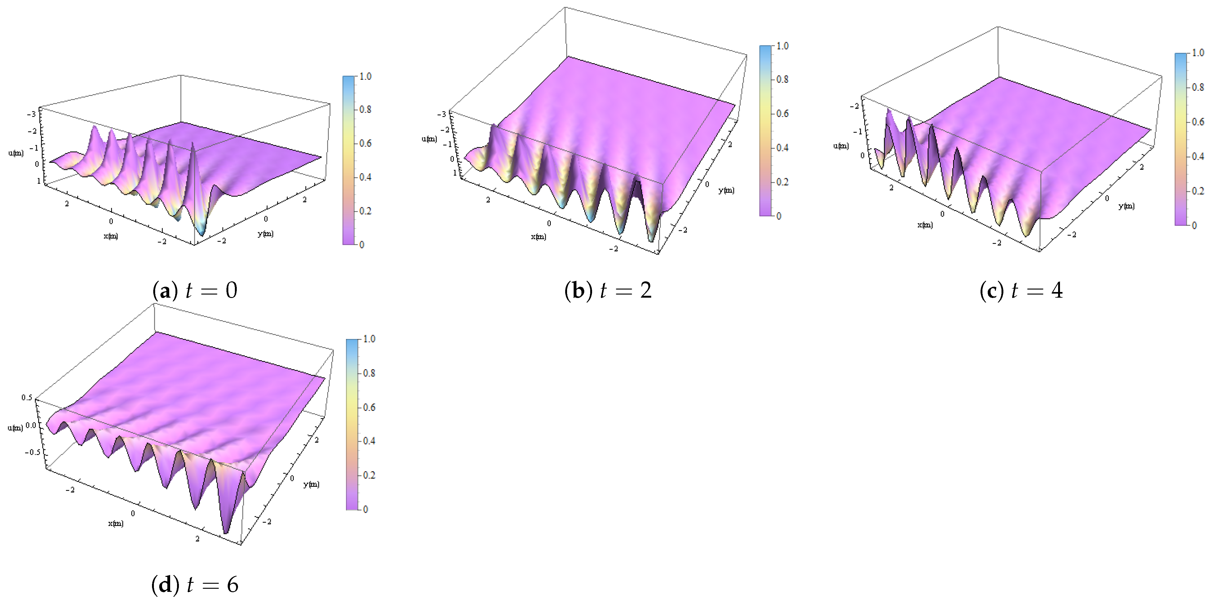
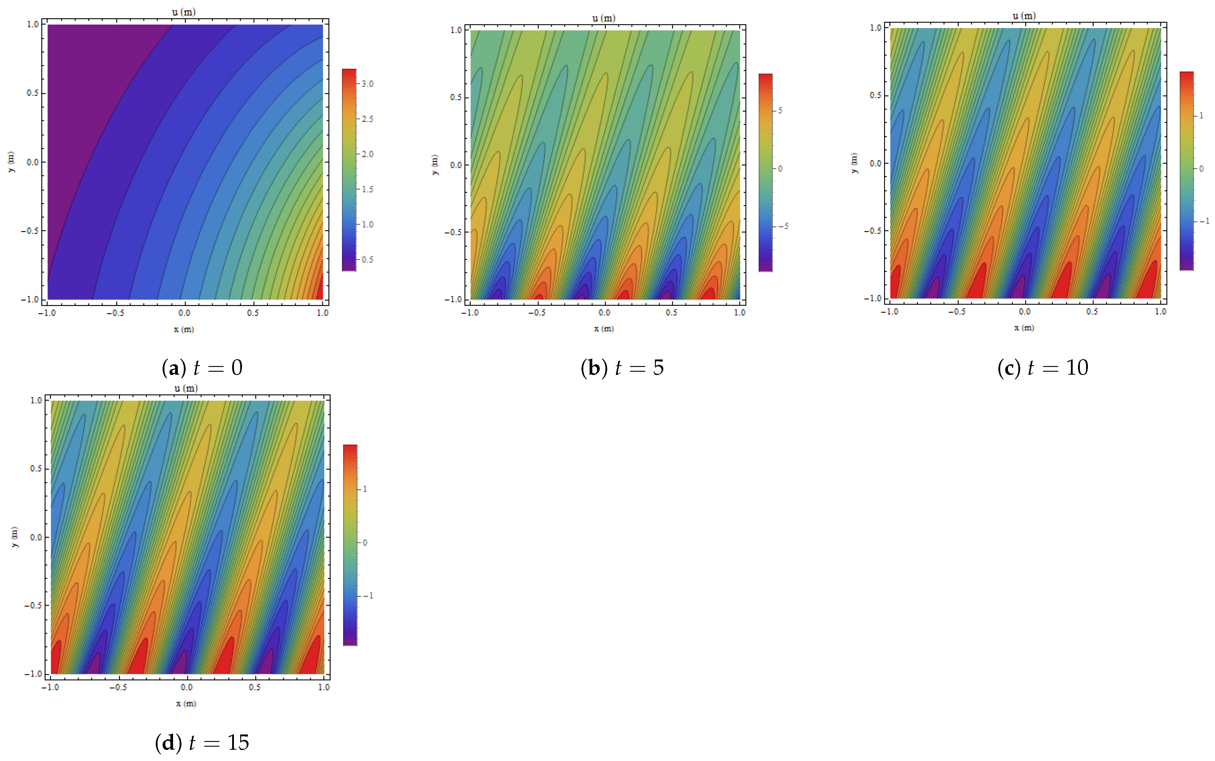
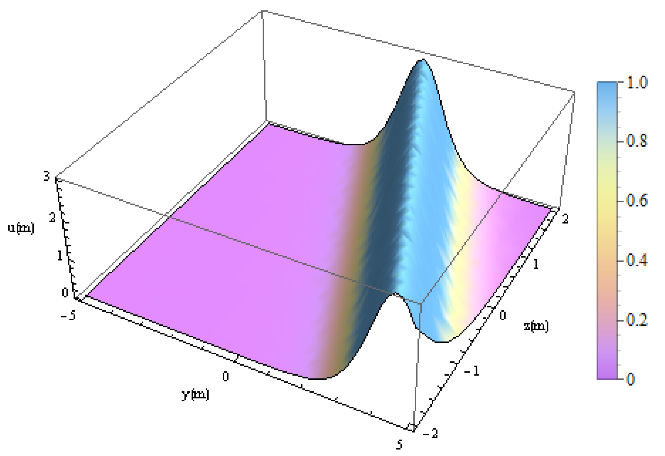
We utilize the transformation in (3), which is provided as [16]

$$f=e^{-i{p}_1\left(a_{1}x+a_{2}y+a_{3}z-k_{1}t\right)}+b_{1}cos\left(p\left(a_{1}x+a_{2}y+a_{3}z+k_{2}t\right)\right)+b_2{e}^{-p_1\left(a_{1}x+a_{2}y+a_{3}z-k_{1}t\right)},$$

(35)

where $a_1,a_2,a_3,k_1,k_2$ are constants. This time, f in (3) is used and the cosine and $exp$ function coefficients are left at zero to obtain the following.

Set I.

$$\begin{array}{c}\hfill \left\{\begin{array}{c}{k}_1=-{\displaystyle \frac{a_1\left(4a_1^2{a}_2{p}^2+a_3\right)}{2a_2}},\hfill \\ p_1=p,\hfill \\ k_2=k_2,\hfill \\ k_3=k_3.\hfill \end{array}\right.\end{array}$$

(36)

These parameters, via (36), (35), and (2), imply

$$\begin{array}{c}\hfill u_{12}=-{\displaystyle \frac{3\left(B_1+b_{1}cos\left(p\left(\frac{a_1\left(4a_1^2{a}_2{p}^2+a_3\right)t}{2a_2}+a_{1}x+a_{2}y+a_{3}z\right)\right)\right)\left(B_2\right)-B_3}{{\left(B_1+b_{1}cos\left(p\left(\frac{a_1\left(4a_1^2{a}_2{p}^2+a_3\right)t}{2a_2}+a_{1}x+a_{2}y+a_{3}z\right)\right)\right)}^2}},\end{array}$$

(37)

where $B_1=e^{-ip\left({\displaystyle \frac{a_1\left(4a_1^2{a}_2{p}^2+a_3\right)t}{2a_2}}+a_{1}x+a_{2}y+a_{3}z\right)}+b_2{e}^{ip\left({\displaystyle \frac{a_1\left(4a_1^2{a}_2{p}^2+a_3\right)t}{2a_2}}+a_{1}x+a_{2}y+a_{3}z\right)}$,

$B_2=D_1-a_1^2{b}_1{p}^{2}cos\left(p\left({\displaystyle \frac{a_1\left(4a_1^2{a}_2{p}^2+a_3\right)t}{2a_2}}+a_{1}x+a_{2}y+a_{3}z\right)\right)$,

$D_1=-a_1^2{e}^{-ip\left({\displaystyle \frac{a_1\left(4a_1^2{a}_2{p}^2+a_3\right)t}{2a_2}}+a_{1}x+a_{2}y+a_{3}z\right)}--a_1^2{b}_2{p}^2{e}^{ip\left({\displaystyle \frac{a_1\left(4a_1^2{a}_2{p}^2+a_3\right)t}{2a_2}}+a_{1}x+a_{2}y+a_{3}z\right)}$ and

$B_3=D_1-a_1^2{b}_1{p}^{2}cos\left(p\left({\displaystyle \frac{a_1\left(4a_1^2{a}_2{p}^2+a_3\right)t}{2a_2}}+a_{1}x+a_{2}y+a_{3}z\right)\right)$.

11. GBs

We utilize the transformation in (3), which is provided as [16]

$$f={\displaystyle \frac{\left(1-4c\right)cosh\left(a_{1}t\right)+\sqrt{2c}cos\left(a_{2}x+a_{3}y+a_{4}z\right)+a_{1}sinh\left(a_{1}t\right)}{\sqrt{2c}cos\left(a_{2}x+a_{3}y+a_{4}z\right)-cosh\left(a_{1}t\right)}},$$

(38)

where $a_1,a_2,a_3,a_4,c$ are constants. This time, f in (3) is used and the cosine, hyperbolic, and $exp$ function coefficients are left at zero to obtain the following.

Set I.

$$\begin{array}{c}\hfill a_4=-{\displaystyle \frac{4a_3{a}_2^2}{3}},c={\displaystyle \frac{1}{2}},k_2=k_2,a_3=a_3\end{array}$$

(39)

These parameters, via (39), (38), and (2), give

$$\begin{array}{c}\hfill u_{13}=-{\displaystyle \frac{3\left(cos\left(a_{2}x+a_{3}y-\frac{4a_2^2{a}_3}{3}z\right)\left(-\frac{a_{2}sin\left(a_{2}x+a_{3}y-\frac{4a_2^2{a}_3}{3}z\right)}{cos\left(a_{2}x+a_{3}y-\frac{4a_2^2{a}_3}{3}z\right)-cosh\left(a_{1}t\right)}+E_1\right)\right)}{cos\left(a_{2}x+a_{3}y-\frac{4a_2^2{a}_3}{3}z\right)-cosh\left(a_{1}t\right)+a_{1}sinh\left(a_{1}t\right)}},\end{array}$$

(40)

where the value of $E_1$ is

$$\begin{array}{c}\hfill E_1={\displaystyle \frac{a_{2}sin\left(a_{2}x+a_{3}y-\frac{4a_2^2{a}_3}{3}z\right)\left(cos\left(a_{2}x+a_{3}y-\frac{4a_2^2{a}_3}{3}z\right)-cosh\left(a_{1}t\right)+a_{1}sinh\left(a_{1}t\right)\right)}{{\left(cos\left(a_{2}x+a_{3}y-\frac{4a_2^2{a}_3}{3}z\right)-cosh\left(a_{1}t\right)\right)}^2}}.\end{array}$$

(41)

12. Symbolic Computation with Ansatz Function Technique

In the upcoming sections, we find the solitary waves (SWs) for the governing equation. We compute amplitude, speed, energy relation, pressure relation, thickness, and safety factor for coastal structures via the ansatz function technique. The ansatz function methodology is a potent tool for locating exact solutions to complicated problems, particularly differential equations, in a variety of disciplines, including applied mathematics, engineering, and physics. This method gains even more power when coupled with symbolic computation, enabling the symbolic, instead of numerical, manipulation and solution of mathematical problems [25].

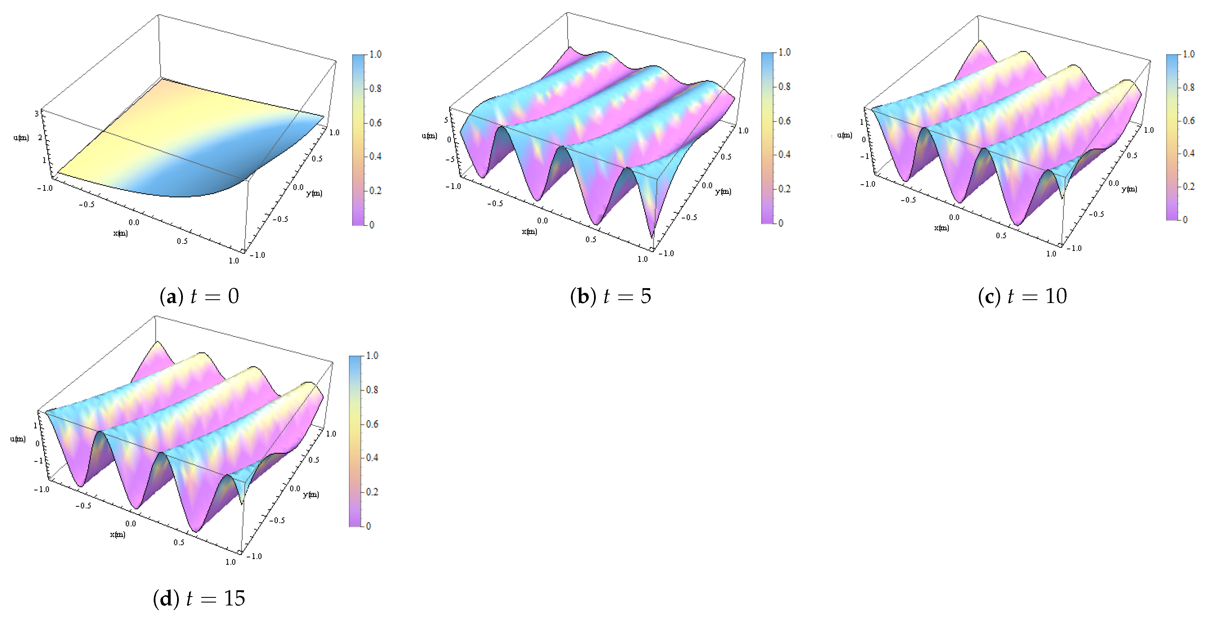
13. Solitary Waves (SWs)

We use the following ansatz [26,27,28]:

$$u(x,y,z,t)=\psi \left(\xi \right),\xi =kx+ly+mz-ct,$$

(42)

where k, l, m are constants related to the wave numbers and c represents the speed of the wave. Using (42) in (1), we obtain the following equation:

$$4kl{\psi }^{{}^{\prime }2}\left(\xi \right)+2cl{\psi }^{″}\left(\xi \right)+3km{\psi }^{″}\left(\xi \right)+4kl\psi \left(\xi \right){\psi }^{″}\left(\xi \right)-2k^{3}l{\psi }^{\left(iv\right)}\left(\xi \right)=0.$$

(43)

For a solitary wave, assume

$$\psi \left(\xi \right)=Asec{h}^2\left(B\xi \right),$$

(44)

where A represents the amplitude and B is related to the width of the wave. By using (44) in (43) and by balancing terms with respect to various powers of hyperbolic functions, we isolate coefficients. After solving these equations, we obtain the SWs as follows:

$$u\left(x,y,z,t\right)=-3B^2{k}^{2}sech{\left[B\left(-{\displaystyle \frac{k\left(4B^2{k}^{2}l-3m\right)t}{2l}}+kx+ly+mz\right)\right]}^2.$$

(45)

The amplitude A of the wave is given by

$$A=3B^2{k}^2$$

(46)

The speed c of the wave is calculated as

$$c={\displaystyle \frac{k\left(4B^2{k}^{2}l-3m\right)}{2l}}$$

(47)

To establish a meaningful correspondence between the parameters in the ansatz and real ocean conditions, it is essential to link the abstract mathematical parameters k, l, m, c, A, B with physical quantities observed in the ocean. The ansatz for the wave profile in (42) is a traveling wave solution, where k, l, m are constants associated with the wave numbers in the x, y, and z directions. They define the spatial scales of the wave. c is wave speed, which represents how fast the wave propagates in the x, y, and z domains. Meanwhile, $\psi \left(\xi \right)$ describes the wave shape in terms of $sec{h}^2\left(\xi \right)$, which is common for solitary wave profiles. Physically, k, l, m wave numbers are inversely related to the wavelength in each direction. The values of $k={\displaystyle \frac{2\pi }{{\lambda }_x}}$, $l={\displaystyle \frac{2\pi }{{\lambda }_y}}$, and $m={\displaystyle \frac{2\pi }{{\lambda }_z}}$ are wavelengths along their respective axes. In oceanic solitary waves, ${\lambda }_x$ might represent the longitudinal wavelength, and ${\lambda }_y$, ${\lambda }_z$ could model transverse spreading or depth dependence. The amplitude $A=3B^2{k}^2$ is directly proportional to the square of the wave number $k^2$ and the width parameter $B^2$. In physical terms, A corresponds to the maximum height of the solitary wave relative to the undisturbed surface or interface (e.g., pycnocline for internal waves). In oceanic terms, B reflects the steepness or sharpness of the wave, controlled by factors like stratification or nonlinearity. The speed $c={\displaystyle \frac{k\left(4B^2{k}^{2}l-3m\right)}{2l}}$ depends on the interplay between nonlinearity $B^2{k}^2$, stratification effects l, and the vertical wave number m. In physical terms, c can vary due to changes in water depth, density gradients, or external forces like currents. As a real-world example, consider internal solitary waves in the South China Sea: the observed characteristics are amplitude $A\sim 100$ m, width ${\lambda }_x\sim 5$ km, speed $c\sim 2$ m/s, depth $H\sim 200$ m. After matching the parameters $k={\displaystyle \frac{2\pi }{5000}}$ m⁻¹, $B \propto pycnoclinethickness$, if we tune the parameters to $k=2$, $B=1$, $l=0.34375$, $m=1$ in (47), then we obtain the value of $c=2$ m/s, which matches the speed of internal solitary waves in the South China Sea [29]. Understanding nonlinear waves, particularly strong waves, is crucial for determining how they affect underwater vehicles and offshore oil rigs, as well as for comprehending how they affect changes in marine ecosystems and fishing activity. Particularly in the northern South China Sea (SCS), the Sulu Sea, the Andaman Sea, the Washington Shelf, the North West Shelf of Australia, the Strait of Gibraltar, and Massachusetts Bay, nonlinear waves are active in marginal seas. According to field research, waves in these areas frequently have amplitudes between 10 and 100 m. As far as the authors are aware, the northern SCS has the strongest waves among the world’s oceans that have ever been recorded [29].

14. Energy of the Wave

The total energy E of the wave can be calculated using the kinetic and potential energy contributions. For a solitary wave, the total energy per unit length is typically expressed as follows [26,27,28,30,31,32].

The kinetic energy $KE$ is typically calculated as

$$KE=\underset{-\infty }{\overset{\infty }{\int }}{\displaystyle \frac{1}{2}}u{\left(\xi \right)}^{2}d\xi =3B^3{k}^4$$

(48)

The potential energy $PE$ is typically calculated as

$$PE=\underset{-\infty }{\overset{\infty }{\int }}{\displaystyle \frac{1}{2}}{\left({\displaystyle \frac{\partial u\left(\xi \right)}{\partial t}}\right)}^{2}d\xi =-{\displaystyle \frac{4A^{2}B}{15}}{\left({\displaystyle \frac{k\left(4B^2{k}^{2}l-3m\right)}{2l}}\right)}^2$$

(49)

The total energy E is the sum of $PE$ and $KE$, calculated by using (48) and (49):

$$E=KE+PE=3B^3{k}^4-{\displaystyle \frac{4A^{2}B}{15}}{\left({\displaystyle \frac{k\left(4B^2{k}^{2}l-3m\right)}{2l}}\right)}^2$$

(50)

Energy of the Rogue Wave

The total energy E of the wave can be calculated using the kinetic and potential energy contributions. For an RW $u_5$, we put $y=0$, $z=0$ and choose time $t=0$ (for the sake of simplicity) [26,27,28,30].

The $KE$ is calculated as

$$KE={\displaystyle \frac{1}{2}}\underset{-\infty }{\overset{\infty }{\int }}{u}_5^{2}dx$$

(51)

To proceed numerically with these integrals, let us assign specific values to the parameters $a_1=0.32$, $a_5=2$, $a_6=1$, $a_{10}=0.5$, $a_{11}=1$, $b_1=0.1$, $k_1=0.2$. Integrating over the range of $x=-10$ to $x=10$, using (51) and (16), we obtain $KE=1.90614$, which is approximately equal to the $KE$ of the wave given in [29]. The $PE$ is calculated as

$$PE={\displaystyle \frac{1}{2}}\underset{-\infty }{\overset{\infty }{\int }}{\left({\displaystyle \frac{\partial u_5}{\partial x}}\right)}^{2}dx$$

(52)

With $a_1=0.32$, $a_5=2$, $a_6=1$, $a_{10}=0.5$, $a_{11}=1$, $b_1=0.1$, $k_1=0.2$ and integrating over the range of $x=-10$ to $x=10$, using (52) and (16), we obtain $PE=1.51788$, which is approximately equal to the $PE$ of the wave given in [29]. The total energy E is the sum of $PE$ and $KE$, calculated by using (48) and (49):

$$E=KE+PE=1.90614+1.51788=3.42402\mathrm{J}/\mathrm{m}$$

(53)

15. Discussions

We have computed multiple dark and bright lump waves for the model that is used in shallow-water waves. In Figure 1, we represent the 3D bright and dark lump wave propagations for solution $u_2(x,y,z,t)$ (8) with $a_2=5, a_3=20, a_4=7$, $a_5=50$, $a_6=-2$, $a_7=10, a_8=2, a_9=3, a_{10}=11, a_{11}=4, z=0$, and different t. There is one dark lump wave and two bright lump waves with noticeably larger amplitudes at (a) $t=1$ and (b) $t=5$; they retain their shapes as they were prior to interaction. At (c) $t=10$, two bright LW and two dark lump waves with different amplitudes occur. At (d) $t=15$, a single bright LW and two dark LWs slightly changes their amplitudes. A lump wave, which frequently resembles a single, solitary hump on the water’s surface, is a concentrated energy package with a distinct peak. Like solitons, lump waves maintain their structure as they move. A balance between nonlinear steepening and dispersive spreading results in lump waves. In shallow water, nonlinearity tends to steepen and amplify waves, whereas dispersion permits them to spread out horizontally. Because of this equilibrium, a steady, limited wave structure that moves without altering shape is maintained.

Figure 2 illustrates the contour propagation of the solution $u_2(x,y,z,t)$ in (8) with the parameter values $a_2=5, a_3=20, a_4=7$, $a_5=50$, $a_6=-2, a_7=10, a_8=2, a_9=3$, $a_{10}=11, a_{11}=4$, and $z=0$ for different values of t. In this plot, the center of the lump wave is shown as a high-amplitude peak; in a color-coded contour map, this is typically shown as the innermost contour line or a bright, concentrated color. This peak indicates the wave’s highest energy concentration. As one moves outside from the center, the wave amplitude gradually decreases, as indicated by the contour lines surrounding the peak. The oval or concentric patterns formed by these contours demonstrate the lump wave’s restricted nature. As one moves further away from the center, the contour levels increase smaller, indicating a drop in amplitude. In Figure 3, we present 3D bright–dark lump structures combined with periodic wave propagations for the solution $u_4(x,y,z,t)$ given in Equation (13). This visualization is generated using the parameter values $a_3=20, a_4=7, a_5=50, a_6=-2, a_7=10, a_8=2, a_9=3, a_{10}=11, a_{11}=4, k_1=-7$, $k_2=3, k_3=5, k_4=4, b_1=1,$ and $z=0$ for various values of t. At (a) $t=0$, multiple bright lumps with periodic waves are present, with one having a significantly higher amplitude, while others exhibit smaller amplitudes; (b) $t=2,$ multiple bright (LWs) interact with each other, one having a significantly higher amplitude afterward, while others exhibit smaller amplitudes; (c) $t=4$, multiple bright (LWs) with various amplitudes, the first bright LWs having smaller amplitude; (d) $t=6$, the first three bright LWs have smaller amplitudes, while others exhibit larger amplitudes. A spatially concentrated peak, resembling a lump, that occurs frequently along one or more spatial directions is observed in LPs. These waves can transmit localized energy concentrations over periodic patterns due to their hybrid structure. This can suggest fluctuating energy concentrations at various locations and times, which makes them especially interesting in shallow-water dynamics. LPs in shallow water can be seen as pressure peaks or periodic energy bursts that spread across the water’s surface. The behavior of complex wave interactions and their consequences, such as energy transmission in shallow-water zones, which may affect marine and coastal areas, can be studied with the help of these waveforms.

Figure 4 illustrates the contour plot of a bright–dark lump accompanied by periodic wave propagations for the solution $u_4(x,y,z,t)$ to (13). The parameters are selected as $a_3=20, a_4=7, a_5=50, a_6=-2, a_7=10, a_8=2, a_9=3, a_{10}=11, a_{11}=4, k_1=-7$, $k_2=3, k_3=5, k_4=4, b_1=1, z=0$ and varying t. Areas with higher or lower wave amplitudes are shown by the contour lines. These contours demonstrate the concentration of energy in particular areas by exposing localized peaks that occur periodically throughout the spatial domain in the case of a lump periodic wave. Repeated clusters of contours, each around a peak (or lump), indicate the wave’s periodic character. The organized, periodic character of the wave in different directions is represented by the pattern that these clusters create, which repeats at regular intervals. Figure 5 illustrates the 3D propagation of rogue waves, featuring bright and dark lump waves (LWs) for the solution $u_5(x,y,z,t)$ given in Equation (16). The solution is visualized with the parameter selection $a_1=2, a_3=-10, a_4=7, a_5=5, a_6=-2, a_7=10, a_8=2, a_9=3, a_{10}=11, a_{11}=4$, $k_2=3, k_3=5, k_4=4$, $z=0$, and at various values of t. We observe, at (a) $t=0$, RWs having zero-amplitude, and (b) $t=5,$ RWs having high-amplitude peaks that appear as isolated, abrupt elevations in the water surface; (c) $t=10$, RWs having high-amplitude peaks that appear as isolated, abrupt elevations in the water surface; (d) $t=15$, RWs having high-amplitude peaks that appear as isolated, abrupt elevations in the water surface. An RW is distinguished by its amplitude, with wave heights frequently reaching twice the significant wave height. When many wave groups constructively overlap, RWs can occur, producing sudden peaks with abnormally large amplitudes. This constructive interference can create extreme waves in shallow water, where waves have higher amplitudes and shorter wavelengths. The contour plots of rogue wave propagation for the solution $u_5(x,y,z,t)$ in (16) are depicted in Figure 6. These visualizations were generated using the parameter values $a_1=2, a_3=-10,$$a_4=7, a_5=5, a_6=-2, a_7=10, a_8=2, a_9=3, a_{10}=11, a_{11}=4, k_2=3, k_3=5, k_4=4$ with $z=0$ and varying t. The contour lines illustrate a progressive amplitude decay in the surrounding wave field as one moves away from the peak, becoming further scattered. This spread shows how the wave’s energy decreases as it moves into nearby regions. With the greatest amplitude in its core, the wave’s highest point manifests as a clear, tightly enclosed contour. The peak, which is usually a bright area, is the core of the RW.

Figure 7 interprets the L1kI profiles for $u_7(x,y,z,t)$ in (21) via $a_1=2, a_2=3, a_3=2,$$a_4=7, a_5=5, a_6=-2, a_7=10, a_9=3, a_{10}=11, a_{11}=4, k_2=3, k_3=5, k_4=4, x=0$. At (a) $t=0$, one bright LW interacts with one-stripe waves; (b) $t=2,$ after their interaction, the amplitude of the strip wave suddenly increases; (c) $t=4$, the stripe waves become more prominent, having larger amplitude. Single, localized wave packets with a spatial profile resembling a stripe are known as one-stripe solitons. They are simpler than lump solitons and usually feature a single peak. An initial wave configuration consisting of a lump soliton and a one-stripe soliton is used to initiate the interaction. The type of interaction between the solitons can be affected by their initial shapes, amplitudes, and speeds. The profile of the one-strip soliton may be distorted by the lump soliton during the contact. The one-strip soliton’s amplitude and velocity may alter as a result of the lump. The one-stripe soliton’s properties can be changed by transferring the energy from the lump soliton to it. And Figure 8 shows L2kI profiles for $u_8(x,y,z,t)$ in (24) via $a_1=2, a_2=3, a_3=2, a_4=7$, $a_5=5, a_6=-2, a_7=10, a_9=3, a_{10}=11, a_{11}=4, k_2=3, k_3=5, k_4=4, x=0$. At (a) $t=0$, two bright LWs interact with one-strip waves; (b) $t=2,$ after their interaction, we obtain one bright LW and a strip wave; (c) $t=4$, the stripe wave becomes more prominent, having larger amplitude. The two-stripe soliton’s amplitude and velocity may alter as a result of the lump. The two-stripe soliton’s properties can be changed by transferring the energy from the lump soliton to it.

The interaction between lump, periodic, and strip-wave profiles for $u_9(x,y,z,t)$ in (28) are constructed in Figure 9 via $a_1=2, a_2=3, a_3=2, a_4=7, a_5=5, a_6=-2, a_7=10$, $a_9=3, a_{10}=11, a_{11}=4, k_2=3, k_3=5, k_4=4, x=0, t=0$. At (a) $t=0$, multiple LP waves and a stripe wave interact with each other; (b) $t=2,$ after their interaction, both these waves merge into a strip wave having significant amplitude; (c) $t=4$, a stripe wave having significant amplitude. The interaction between LP, RW, and stripe wave profiles for $u_{10}(x,y,z,t)$ in (31) are constructed in Figure 10 via $a_1=2, a_2=3, a_3=2, a_4=7$, $a_5=5, a_6=-2, a_7=10, a_9=3, a_{10}=11, a_{11}=4, k_2=3$, $k_3=5, k_4=4, k_6=2, k_7=1$, $k_8=1.5,b_1=2, b_2=4, x=0, t=0$. At (a) $t=0$, butterfly waves, (b) $t=2,$X waves, (c) $t=4$; two stripe waves having significant equal amplitudes. Usually, butterfly waves have a symmetrical, characteristic shape that is similar to butterfly wings. This form may arise as a result of wave packet interaction or under particular circumstances, such as modulation and wave focusing. Butterfly waves can have profiles with several peaks, characterized by narrow valleys and dispersed crests that resemble wings. Butterfly waves are frequently created when various wave trains collide with one another. The intricate, nonlinear interactions that result from the intersection of waves with different wavelengths and velocity can create the butterfly pattern. Studying the geometry of X-waves in shallow water is interesting because of the potential applications to coastal engineering and wave dynamics. One sort of nonlinear wave structure known as an X-wave is distinguished by its unusual shape, which is similar to the letter X. They can happen in different depths of water, but, because of the effects of nonlinearity and dispersion, they are more important in shallow water.

Figure 11 represents the MB profiles for $u_{11}(x,y,z,t)$ in (43) with the choice of $a_1=1.5$, $a_2=2, k_2=1.5, b_1=-3, x=0$. The amplitude of MBs varies along the longitudinal axis, which is frequently linked to time, and it exhibits a periodic oscillation structure in time while being localized in space. The MB’s geometry can appear in shallow water as a series of gradually growing and shrinking wave crests and troughs. The RW linked to the MB manifests as a highly localized peak in the shallow-water environment. The Ma breather’s maximum amplitude point, which denotes the extreme limit where the breather’s oscillations collapse into a single, isolated wave, is typically where the RW is centered. The MB and its related RW characterize the energy concentration and dispersion dynamics in shallow water, which are essential for forecasting wave patterns that may have an impact on coastal regions. In the mean time, KMB profiles for $u_{12}(x,y,z,t)$ in (37) are constructed in Figure 12 via $a_2=2, a_3=2, b_1=4, p=5, b_2=1.2, x=0, t=0$. Wave dynamics, usually in deep water, are captured by the KMB, a periodic, localized solution of the nonlinear partial differential equation. Its geometry exhibits a confined, localized structure with sharp peaks and troughs formed by periodic concentrations and decays in wave amplitude. Because it can simulate the temporary amplification of waves that results in RW production, this breather is frequently linked to RW events. The GB profiles for $u_{13}(x,y,z,t)$ in (40) are constructed via $a_1=1.5, a_2=3, a_3=2, a_4=3$, $k_1=1.5, x=0$ in Figure 13. The SW profiles for $u(x,y,z,t)$ in (45) are constructed via $k=1, l=1, m=1, B=1, x=0, t=0$ in Figure 14. Even when traveling long distances or after interacting with other waves, solitary waves retain their shape and speed. Since a single wave’s speed rises with its amplitude compared to regular waves, higher waves can carry more energy and move faster. Coastal structures like levees, piers, breakwaters, and seawalls are particularly susceptible to the risks and difficulties posed by solitary waves. The height of solitary waves is frequently greater than their length. Significant wave run-up, or the movement of water up the surface of a coastal structure, can occur when such a wave strikes it. Over-topping, in which water runs over the structure, can result from high run-up and could cause erosion and floods.

16. Conclusions

Using Hirota bilinear and Cole–Hopf transformation techniques, a class of new results for the (3 + 1)-dimensional nonlinear Geng equation have been developed in this paper. In shallow-water waves, the governing model can be applied to represent more intricate wave dynamics. Some properties of wave dynamics can be explained by their solutions. Computing the bright and dark lump wave solutions has been significantly aided by the quadratic polynomial function in the bilinear equation. We have studied that, by appropriately changing the parameter groups in the lump solutions, Equation (1) has various lump waves, including bright and dark lump waves. We also talked about the interactions between soliton and numerous lump waves. The lump one-strip solutions are obtained by applying a combination of positive quadratic and exponential transformations to the governing equation. By combining positive quadratic and exponential transformations on the governing equation, the lump two-strip solutions are calculated. Positive quadratic transformation and cosine are combined to calculate the RWs. RWs usually have crests that are much higher than the waves in their immediate vicinity. They rise to a minimum of 30 m (or 100 feet), more than twice as high as the nearby waves. The same periodic solutions are also found by a cosine and positive quadratic hyperbolic transformation. Numerous interactions are computed, such as L1SI, L1SI, LP, lump wave, and rogue waves. The MBs, KMBs, and GBs are successfully computed together with the related RWs. Additionally, we have evaluated mixed solutions with butterfly waves, X-waves, and lump waves. Furthermore, we have SWs and build a relation between the energy of the wave on coastal structures via the ansatz function technique. The energy associated with rogue waves, solitary waves, and higher-amplitude waves is significant and have catastrophic effects on coastal structures. Proper design strategies, including reinforced foundations, energy dissipation techniques, and accurate forecasting, are essential for constructing resilient coastal infrastructure capable of withstanding extreme wave events. Fractal characteristics in RWs, solitons, multi-soliton solutions, chaotic solutions, and breather interactions often emerge from the complex interplay of dispersion, nonlinearity, and parametric values inherent in the governing equation. RWs, solitons, nonlinear waves, and breathers interact in ways that produce nested, self-replicating structures. Solitons of different amplitudes and speeds create nested structures that show fractal properties. In summary, fractal characteristics in these nonlinear phenomena reflect the underlying complexity and interplay of mathematical structures, offering insights into energy transfer, wave characteristics, and multi-scale dynamics in physical systems.

References

1. Bertoldi, K.; Vitelli, V.; Christensen, J.; Van Hecke, M. Flexible mechanical metamaterials. Nat. Rev. Mater. 2017, 11, 1–11. [Google Scholar] [CrossRef]
2. Holmes, D.P. Elasticity and stability of shape-shifting structures. Curr. Opin. Colloid Interface Sci. 2019, 40, 118–137. [Google Scholar] [CrossRef]
3. Deng, B.; Raney, J.R.; Tournat, V.; Bertoldi, K. Elastic vector solitons in soft architected materials. Phys. Rev. Lett. 2017, 18, 204102. [Google Scholar] [CrossRef] [PubMed]
4. Deng, B.; Wang, P.; He, Q.; Tournat, V.; Bertoldi, K. Metamaterials with amplitude gaps for elastic solitons. Nat. Commun. 2018, 9, 3410. [Google Scholar] [CrossRef]
5. Raney, J.R.; Nadkarni, N.; Daraio, C.; Kochmann, D.M.; Lewis, J.A.; Bertoldi, K. Stable propagation of mechanical signals in soft media using stored elastic energy. Proc. Natl. Acad. Sci. USA 2016, 113, 9722–9727. [Google Scholar] [CrossRef]
6. Edelman, M. Comments on A note on stability of fractional logistic maps. Appl. Math. Lett. 2022, 125, 107787. [Google Scholar]
7. Shen, S.; Yang, Z.J.; Pang, Z.G.; Ge, Y.R. The complex-valued astigmatic cosine-Gaussian soliton solution of the nonlocal nonlinear Schrödinger equation and its transmission characteristics. Appl. Math. Lett. 2022, 125, 107755. [Google Scholar] [CrossRef]
8. Song, L.M.; Yang, Z.J.; Li, X.L.; Zhang, S.M. Coherent superposition propagation of Laguerre–Gaussian and Hermite–Gaussian solitons. Appl. Math. Lett. 2020, 102, 106114. [Google Scholar] [CrossRef]
9. Shen, S.; Yang, Z.; Li, X.; Zhang, S. Periodic propagation of complex-valued hyperbolic-cosine-Gaussian solitons and breathers with complicated light field structure in strongly nonlocal nonlinear media. Commun. Nonlinear Sci. Numer. Simul. 2021, 103, 106005. [Google Scholar] [CrossRef]
10. Yi, H.; Yao, Y.; Zhang, X.; Ma, G. High-order effect on the transmission of two optical solitons. Chin. Phys. B 2023, 32, 100509. [Google Scholar] [CrossRef]
11. Li, X.L.; Guo, R. Interactions of Localized Wave Structures on Periodic Backgrounds for the Coupled Lakshmanan–Porsezian–Daniel Equations in Birefringent Optical Fibers. Ann. Phys. 2023, 535, 2200472. [Google Scholar] [CrossRef]
12. Ahmed, S.; Seadawy, A.R.; Rizvi, S.T. Study of breathers, rogue waves and lump solutions for the nonlinear chains of atoms. Opt. Quantum Electron. 2022, 4, 1–28. [Google Scholar] [CrossRef]
13. Seadawy, A.R.; Rizvi, S.T.; Ahmed, S. Weierstrass and Jacobi elliptic, bell and kink type, lumps, Ma and Kuznetsov breathers with rogue wave solutions to the dissipative nonlinear Schrödinger equation. Chaos Solitons Fractals 2022, 160, 112258. [Google Scholar] [CrossRef]
14. Seadawy, A.R.; Rizvi, S.T.; Ahmed, S. Multiple lump, generalized breathers, Akhmediev breather, manifold periodic and rogue wave solutions for generalized Fitzhugh-Nagumo equation: Applications in nuclear reactor theory. Chaos Solitons Fractals 2022, 161, 112326. [Google Scholar] [CrossRef]
15. Ma, Y.L. N-solitons, breathers and rogue waves for a generalized Boussinesq equation. Int. J. Comput. Math. 2020, 97, 1648–1661. [Google Scholar] [CrossRef]
16. Seadawy, A.R.; Rizvi, S.T.; Ahmed, S.; Bashir, A. Lump solutions, Kuznetsov–Ma breathers, rogue waves and interaction solutions for magneto electro-elastic circular rod. Chaos Solitons Fractals 2022, 163, 112563. [Google Scholar] [CrossRef]
17. Hietarinta, J. Introduction to the Hirota bilinear method. In Integrability of Nonlinear Systems; Springer: Berlin/Heidelberg, Germany, 1997; Volume 1, pp. 95–103. [Google Scholar]
18. Zuo, J.M.; Zhang, Y.M. The Hirota bilinear method for the coupled Burgers equation and the high-order Boussinesq—Burgers equation. Chin. Phys. B 2011, 20, 010205. [Google Scholar] [CrossRef]
19. Liu, Y.; Wen, X.Y.; Wang, D.S. The N-soliton solution and localized wave interaction solutions of the (2+1)-dimensional generalized Hirota-Satsuma equation. Comput. Math. Appl. 2019, 77, 947–966. [Google Scholar] [CrossRef]
20. Li, B.Q.; Ma, Y.L. Hybrid soliton and breather waves, solution molecules and breather molecules of a (3 + 1)-dimensional Geng equation in shallow water waves. Phys. Lett. A 2023, 52, 106822. [Google Scholar] [CrossRef]
21. Ahmed, S.; Seadawy, A.R.; Rizvi, S.T.; Mubaraki, A.M. Homoclinic breathers and soliton propagations for the nonlinear (3 + 1)-dimensional Geng dynamical equation. Results Phys. 2023, 20, 106822. [Google Scholar] [CrossRef]
22. Geng, X. Algebraic-geometrical solutions of some multidimensional nonlinear evolution equations. J. Phys. A Math. Gen. 2003, 36, 2289. [Google Scholar] [CrossRef]
23. Yin, Y.H.; Lü, X.; Ma, W.X. Bäcklund transformation, exact solutions and diverse interaction phenomena to a (3 + 1)-dimensional nonlinear evolution equation. Nonlinear Dyn. 2022, 108, 4181. [Google Scholar] [CrossRef]
24. Bai, C.L.; Zhao, H. Generalized method to construct the solitonic solutions to (3 + 1)-dimensional nonlinear equation. Phys. Lett. A 2006, 354, 428. [Google Scholar] [CrossRef]
25. Ahmed, I.; Seadawy, A.R.; Lu, D. Kinky breathers, W-shaped and multi-peak solitons interaction in (2+1)-dimensional nonlinear Schrödinger equation with Kerr law of nonlinearity. Eur. Phys. J. Plus 2019, 134, 1. [Google Scholar] [CrossRef]
26. Johnson, R.S. A Modern Introduction to the Mathematical Theory of Water Waves; Cambridge University Press: Cambridge, UK, 1997; Volume 1, p. 19. [Google Scholar]
27. Dodd, R.K.; Eilbeck, J.C.; Gibbon, J.D.; Morris, H.C. Solitons and Nonlinear Wave Equations. J. Appl. Math. Mech. 1985, 65, 354. [Google Scholar] [CrossRef]
28. Benjamin, T.B. The stability of solitary waves. Proc. R. Soc. Lond. Math. Phys. Sci. 1972, 328, 153. [Google Scholar]
29. Huang, X.; Chen, Z.; Zhao, W.; Zhang, Z.; Zhou, C.; Yang, Q.; Tian, J. An extreme internal solitary wave event observed in the northern South China Sea. Sci. Rep. 2016, 6, 30041. [Google Scholar] [CrossRef]
30. Beer, F.P.; Johnston, E.R.; DeWolf, J.T.; Mazurek, D.F.; Sanghi, S. Mechanics of Materials; Mcgraw-Hill: New York, NY, USA, 1992. [Google Scholar]
31. American Society of Civil Engineers. Minimum Design Loads and Associated Criteria for Buildings and Other Structures; American Society of Civil Engineers: Reston, VA, USA, 2020. [Google Scholar]
32. Gulvanessian, H.; Calgaro, J.A.; Holický, M. Designers Guide to Eurocode: Basis of Structural Design: EN 1990; ICE Publishing: Washington, DA, USA, 2012. [Google Scholar]
Figure 1. The 3D bright and dark lump wave propagations. The solution u 2 ( x , y , z , t ) to (8) with the selection of a 2 = 5 ,   a 3 = 20 ,   a 4 = 7 ,   a 5 = 50 ,   a 6 = 2 ,   a 7 = 10 ,   a 8 = 2 ,   a 9 = 3 ,   a 10 = 11 ,   a 11 = 4 ,   z = 0 and different t.
Fractalfract 09 00031 g001
Figure 2. The contour propagations for solution u 2 ( x , y , z , t ) in (8) with the selection of a 2 = 5 ,   a 3 = 20 , a 4 = 7 ,   a 5 = 50 ,   a 6 = 2 ,   a 7 = 10 ,   a 8 = 2 ,   a 9 = 3 ,   a 10 = 11 ,   a 11 = 4 ,   z = 0 and different t.
Fractalfract 09 00031 g002
Figure 3. The 3D bright–dark lump with periodic wave propagations for solution u 4 ( x , y , z , t ) in (13) with the choice of a 3 = 20 ,   a 4 = 7 ,   a 5 = 50 ,   a 6 = 2 ,   a 7 = 10 ,   a 8 = 2 ,   a 9 = 3 ,   a 10 = 11   , a 11 = 4 ,   k 1 = 7 ,   k 2 = 3 ,   k 3 = 5 ,   k 4 = 4 ,   b 1 = 1 ,   z = 0 and different t.
Fractalfract 09 00031 g003
Figure 4. The contour bright–dark lump with periodic wave propagations for solution u 4 ( x , y , z , t ) in (13) with the selection of a 3 = 20 ,   a 4 = 7 ,   a 5 = 50 ,   a 6 = 2 ,   a 7 = 10 ,   a 8 = 2 ,   a 9 = 3 ,   a 10 = 11 , a 11 = 4 ,   k 1 = 7 ,   k 2 = 3 ,   k 3 = 5 ,   k 4 = 4 ,   b 1 = 1 ,   z = 0 and different t.
Fractalfract 09 00031 g004
Figure 5. The 3D RW propagations: bright and dark lump waves for solution u 5 ( x , y , z , t ) in (16) with the choice of a 1 = 2 ,   a 3 = 10 ,   a 4 = 7 ,   a 5 = 5 ,   a 6 = 2 ,   a 7 = 10 ,   a 8 = 2 ,   a 9 = 3 , a 10 = 11 , a 11 = 4 ,   k 2 = 3 ,   k 3 = 5 ,   k 4 = 4 ,   z = 0 , and different t.
Fractalfract 09 00031 g005
Figure 6. The contour RW propagations: bright and dark lump waves (LWs) for solution u 5 ( x , y , z , t ) in (16) with the selection of a 1 = 2 ,   a 3 = 10 ,   a 4 = 7 ,   a 5 = 5 ,   a 6 = 2 ,   a 7 = 10 ,   a 8 = 2 , a 9 = 3 , a 10 = 11 ,   a 11 = 4 ,   k 2 = 3 ,   k 3 = 5 ,   k 4 = 4 ,   z = 0 , and different t.
Fractalfract 09 00031 g006
Figure 7. L1kI profiles for u 7 ( x , y , z , t ) in (21) are constructed via a 1 = 2 ,   a 2 = 3 ,   a 3 = 2 ,   a 4 = 7 ,   a 5 = 5 , a 6 = 2 ,   a 7 = 10 ,   a 9 = 3 ,   a 10 = 11 ,   a 11 = 4 ,   k 2 = 3 ,   k 3 = 5 ,   k 4 = 4 ,   x = 0 .
Fractalfract 09 00031 g007
Figure 8. L2kI profiles for u 8 ( x , y , z , t ) in (24) are constructed via a 1 = 2 ,   a 2 = 3 ,   a 3 = 2 ,   a 4 = 7 ,   a 5 = 5 , a 6 = 2 ,   a 7 = 10 ,   a 9 = 3 ,   a 10 = 11 ,   a 11 = 4 ,   k 2 = 3 ,   k 3 = 5 ,   k 4 = 4 ,   x = 0 .
Fractalfract 09 00031 g008
Figure 9. Interaction between lump, periodic, and strip-wave profiles for u 9 ( x , y , z , t ) in (28) are constructed via a 1 = 2 ,   a 2 = 3 ,   a 3 = 2 ,   a 4 = 7 ,   a 5 = 5 ,   a 6 = 2 ,   a 7 = 10 ,   a 9 = 3 ,   a 10 = 11 ,   a 11 = 4 , k 2 = 3 , k 3 = 5 ,   k 4 = 4 ,   x = 0 ,   t = 0 .
Fractalfract 09 00031 g009
Figure 10. Interaction between LP, RW, and strip-wave profiles for u 10 ( x , y , z , t ) in (31) are constructed via a 1 = 2 ,   a 2 = 3 ,   a 3 = 2 ,   a 4 = 7 ,   a 5 = 5 ,   a 6 = 2 ,   a 7 = 10 ,   a 9 = 3 ,   a 10 = 11 ,   a 11 = 4 ,   k 2 = 3 ,   k 3 = 5 , k 4 = 4 ,   k 6 = 2 ,   k 7 = 1 ,   k 8 = 1.5 , b 1 = 2 ,   b 2 = 4 ,   x = 0 ,   t = 0 .
Fractalfract 09 00031 g010
Figure 11. MB profiles for u 11 ( x , y , z , t ) in (43) are constructed via a 1 = 0.5 ,   a 2 = 2.5 ,   a 3 = 10 ,   a 4 = 1 , k 2 = 1.5 ,   b 1 = 0.5 ,   z = 0 .
Fractalfract 09 00031 g011
Figure 12. KMB profiles for u 12 ( x , y , z , t ) in (37) are constructed via a 2 = 2 ,   a 3 = 2 ,   b 1 = 4 ,   p = 5 ,   b 2 = 1.2 ,   x = 0 ,   t = 0 .
Fractalfract 09 00031 g012
Figure 13. GB profiles for u 13 ( x , y , z , t ) in (40) are constructed via a 1 = 1.5 ,   a 2 = 3 ,   a 3 = 2 ,   a 4 = 3 , k 1 = 1.5 , x = 0 ,   t = 2 .
Fractalfract 09 00031 g013
Figure 14. SW profiles for u ( x , y , z , t ) in (45) are constructed via k = 1 ,   l = 1 ,   m = 1 ,   B = 1 ,   x = 0 ,   t = 0 .
Fractalfract 09 00031 g014
Disclaimer/Publisher’s Note: The statements, opinions and data contained in all publications are solely those of the individual author(s) and contributor(s) and not of MDPI and/or the editor(s). MDPI and/or the editor(s) disclaim responsibility for any injury to people or property resulting from any ideas, methods, instructions or products referred to in the content.