Dynamics of Fractional-Order Three-Species Food Chain Model with Vigilance Effect

Abstract

This study examines a Caputo-type fractional-order food chain model, considering the Holling type II functional response with the vigilance effect. The model explores the interaction dynamics of the food chain model, which consists of prey, middle predators, and top predators. Additionally, habitat complexity is integrated into the model, which is assumed to reduce predation rates by lowering the encounter rates between predators and prey. All possible feasible equilibrium points are determined and the stability of our proposed model is explored near the equilibrium points. To support the analytical findings, numerical simulation results are given in terms of time series, phase portraits, and bifurcation diagrams. It is discovered that the proposed model can become more stable under a fractional-order derivative. Moreover, the interplay between the vigilance effect and habitat complexity is shown to influence the existence of stable and periodic dynamics.

1. Introduction

Predators affect prey populations and community dynamics, playing an essential role in forming ecosystems. A three-species predator–prey system was the subject of exploration on the presence of chaos by Hasting and Powell [1]. A crucial element of the description of natural systems’ association is complex networks. Numerous researchers have studied food chain models in great detail because they are one of the most significant predator–prey systems. Several intriguing findings have been obtained, including global stability, persistence, the extinction of top predators, the uniqueness and stability of positive periodic results, and more [2,3,4]. Functional responses, which characterize the rate at which a predator attacks a prey, are the central conception in predator–prey relations. Although there are several types of functional responses (Holling I, Holling II, ratio-dependent, etc.), Holling type II is the most generally employed functional response [5,6,7].

Understanding the evolution of an ecosystem’s species diversity is essential to comprehending food web structure. Ecological systems have been analyzed using several mathematical models. The study of vigilance and habitat complexity in predator–prey relations has become a fascinating study area in theoretical ecology and applied mathematics. Nearly every ecosystem is complex, terrestrial or aquatic. Aquatic habitat complexes include, for instance, seagrass, mangroves, aquatic weeds, coastal zone vegetation, coral reefs, salt marshes, etc. Trials conducted in the field and the laboratory have verified that habitat complexity promotes population persistence by reducing predator–prey contact and accordingly reducing predation rates [8,9,10]. Researchers have become more interested in the study of vigilance in population models in recent times [11,12]. An antipredator survival tactic used by the prey population is vigilance. There are costs associated with vigilance actions, similar to consuming energy or cutting out fitness activities [13]. Today, ecology and psychology make expansive use of the term vigilance. The idea of vigilance is constantly employed by ecologists to estimate the nonlethal effects of predators on their prey [14]. With mathematical models, some academics have investigated how vigilance affects the dynamics of a system [15,16]. Although these models frequently use integer-order derivatives to represent dynamic behaviors, they have offered important insights into predator–prey interactions. However, fractional calculus is being used to develop a more sophisticated method that captures more accurate dynamics of complex systems.

Fractional calculus is currently being studied by several academics in the fields of ecology and applied mathematics [17]. It can be used to simulate a broad range of scientific and engineering challenges. In dynamical systems, the conversion of a differential system with integer-order derivatives into a fractional-order derivative has gained popularity [17,18]. There are several advantages to using fractional-order differential equations to simulate prey–predator relations. Many biological systems have been described using fractional-order mathematical models, which are highly dependent on previous activity [19], dealing with species memory that has been achieved during their life cycle, hereditary characteristics, and more [20]. Nevertheless, a small change in the order might result in significant changes in the behavior of solutions. Integer-order differential equations are not able to quantitatively describe complicated biological processes with nonlinear behavior and long-term memory; instead, fractional-order differential equations can. Due to its tendency to provide present states as the influence of all past biological circumstances, specifically the memory effect, natural modeling using fractional calculus is thought to be close to real-world situations [21,22]. It has also been seen to be an important component in creating a more trustworthy and realistic mathematical model. Because fractional calculus can more correctly and efficiently represent the relevant circumstances, its use in natural models is rapidly expanding among academics [23,24]. In addition, they are nearly related to fractals, which are abundant in natural systems [25,26,27]. A discrete fractional-order system with habitat complexity built in the Caupto sense was considered by the authors of [28]. They showed the existence of Hopf bifurcation for both continuous and discrete models. Similarly, the existence and uniqueness of the solution, along with the number of fractional-order model equilibria and their stability, were determined by the authors of [29,30].

A MATLAB algorithm for solving a fractional-order nonlinear system of differential equations was programmed by Garrappa [31]. This work used $\alpha \in (0,1]$ as the fractional-order derivative and the Caputo fractional-order (CFO) operator. We are seeking to explore the solution of the system solely in ${\mathbb{R}}_{+}^3$ for all $t\ge 0$ because of its biological character, which means that the population density remains positive. While prior research has focused on integer-order models, the dynamics of fractional-order systems have received less attention. The vigilance–food chain model, investigated in [11], focuses on stability and bifurcation outcomes using an integer-order system. However, a model with fractional-order derivatives has yet to be explored. Motivated by this gap, we aim to investigate the dynamics of a fractional-order food chain model that includes vigilance and habitat complexity. This study aims to gain a better understanding of the behavior of the system by collecting memory effects.

The structure of this document is as follows: Section 2 formulates the mathematical model. Section 3 presents some preliminary results. We examine the equilibrium points, their existence, their local stability, and the presence of Hopf bifurcation in Section 4. In Section 5, we describe various numerical simulations to demonstrate the results from the preceding section. With the conclusion in Section 6, we end this work.

2. Mathematical Model

The food chain model in [11], which takes into account the impact of habitat complexity, is given by

$$\begin{array}{ccc}\hfill {\displaystyle \frac{d{X}_1}{dT}}& =& B(1-\rho )X_1-M_1{X}_1-A{X}_1^2-{\displaystyle \frac{P_1{X}_1{X}_2(1-\sigma )(1-\gamma )}{(R_1+(1-\sigma )X_1)(g_1+h_1\rho )}},\hfill \\ \hfill {\displaystyle \frac{d{X}_2}{dT}}& =& {\displaystyle \frac{C_1{P}_1(1-\sigma )X_1{X}_2(1-\gamma )}{(R_1+(1-\sigma )X_1)(g_1+h_1\rho )}}-{\displaystyle \frac{P_2{X}_2{X}_3}{(R_2+X_2)(g_2+h_2\gamma )}}-M_2{X}_2,\hfill \\ \hfill {\displaystyle \frac{d{X}_3}{dT}}& =& {\displaystyle \frac{C_2{P}_2{X}_2{X}_3}{(R_2+X_2)(g_2+h_2\gamma )}}-M_3{X}_3,\hfill \end{array}$$

(1)

with initial conditions $X_1\left(0\right)>0$, $X_2\left(0\right)>0$, and $X_3\left(0\right)>0$, where $X_1\left(T\right)$ is the basal prey’s density, $X_2\left(T\right)$ is the middle predator’s density, and $X_3\left(T\right)$ is the top predator’s density at time instant T. The interpretation of all model parameters is provided in Abbreviations Section. Predation took place in the Holling type II form, which characterizes the rate as an increasing function and a saturation function of the prey and is the most commonly used functional response. When there is no habitat complexity $(c=0)$, predator $X_2$ catches the prey at a maximum rate $P_1$. The predation rate drops to $P_1(1-\sigma )$ when complexity is present; the degree or severity of complexity is denoted by the dimensionless parameter $\sigma$. $\sigma$ has a value between 0 and 1. Specifically, $\sigma =0.4$ suggests that habitat complexity reduces the predation rate by $40\%$ [28]. Accordingly, the system simplifies to the system in [11] if there is no habitat complexity and $\sigma =0$.

To reduce the number of parameters and complexity, we use the following transformation:

$$\begin{array}{c}\hfill x_1={\displaystyle \frac{A{X}_1}{M_1}},x_2={\displaystyle \frac{A{X}_2}{C_1{M}_1}},x_3={\displaystyle \frac{A{X}_3}{C_1{C}_2{M}_1}},t=M_{1}T.\end{array}$$

Then, System (1) reduces to the following form:

$$\begin{array}{ccc}\hfill {\displaystyle \frac{dx}{dt}}& =& b(1-\rho )x_1-x_1-{x_1}^2-{\displaystyle \frac{p_1{x}_1{x}_2(1-\gamma )(1-\sigma )}{(1+r_1(1-\sigma )x_1)(g_1+h_1\rho )}},\hfill \\ \hfill {\displaystyle \frac{dy}{dt}}& =& {\displaystyle \frac{p_1{x}_1{x}_2(1-\gamma )(1-\sigma )}{(1+r_1(1-\sigma )x_1)(g_1+h_1\rho )}}-{\displaystyle \frac{p_2{x}_2{x}_3}{(1+r_2{x}_2)(g_2+h_2\gamma )}}-m_2{x}_2,\hfill \\ \hfill {\displaystyle \frac{dz}{dt}}& =& {\displaystyle \frac{p_2{x}_2{x}_3}{(1+r_2{x}_2)(g_2+h_2\gamma )}}-m_3{x}_3,\hfill \end{array}$$

(2)

with initial conditions $x_1\left(0\right)>0$, $x_2\left(0\right)>0$, and $x_3\left(0\right)>0$, where $m_2={\displaystyle \frac{M_2}{M_1}}$, $m_3={\displaystyle \frac{M_3}{M_1}}$, $p_1={\displaystyle \frac{C_1{P}_1}{A{R}_1}}$, $p_2={\displaystyle \frac{C_1{C}_2{P}_2}{A{R}_2}}$, $r_1={\displaystyle \frac{M}{A{R}_1}}$, and $r_2={\displaystyle \frac{C_1{M}_1}{A{R}_2}}$.

Further, using a fractional-order Caputo-type derivative, we add the fractional-order derivative $\alpha$ to Model (2). The resulting form of the reduced model is then obtained and is given by the following:

$$\begin{array}{ccc}\hfill {\displaystyle \frac{d^{\alpha }{x}_1}{dt}}& =& b(1-\rho )x_1-x_1-{x_1}^2-{\displaystyle \frac{p_1{x}_1{x}_2(1-\gamma )(1-\sigma )}{(1+r_1(1-\sigma )x_1)(g_1+h_1\rho )}},\hfill \\ \hfill {\displaystyle \frac{d^{\alpha }{x}_2}{dt}}& =& {\displaystyle \frac{p_1{x}_1{x}_2(1-\gamma )(1-\sigma )}{(1+r_1(1-\sigma )x_1)(g_1+h_1\rho )}}-{\displaystyle \frac{p_2{x}_2{x}_3}{(1+r_2{x}_2)(g_2+h_2\gamma )}}-m_2{x}_2,\hfill \\ \hfill {\displaystyle \frac{d^{\alpha }{x}_3}{dt}}& =& {\displaystyle \frac{p_2{x}_2{x}_3}{(1+r_2{x}_2)(g_2+h_2\gamma )}}-m_3{x}_3,\hfill \end{array}$$

(3)

with initial conditions $x_1\left(0\right)>0$, $x_2\left(0\right)>0$, $x_3\left(0\right)>0$, and $\alpha \in (0,1)$.

3. Preliminaries

We provide the following definitions and theorems regarding the fractional-order differential equation to strengthen our theoretical investigation.

Definition 1.

The fractional derivative in the Caupto sense [32] is given by

$$\begin{array}{c}\hfill D_t^{\alpha }=I^{l-\alpha }{f}^l\left(t\right),\alpha >0,\end{array}$$

provided that l is the least integer that is not smaller than α and that $I^{\theta }$ is the Riemann–Liouville integral operator of order θ, which is given by

$$\begin{array}{c}\hfill I^{\theta }x\left(t\right)={\displaystyle \frac{1}{\Gamma \left(\theta \right)}}{\int }_0^t{(t-\tau )}^{\theta -1}x\left(\tau \right)d\tau ,\theta >0,\end{array}$$

where $\Gamma \left(\theta \right)$ is Euler’s Gamma function and $D^{\alpha }$ is the Caputo fractional operator.

Theorem 1.

By [33], let us consider the fractional differential system of N-dimension ${\displaystyle \frac{d^{\alpha }{x}_1}{d{t}^{\alpha }}}=\mathcal{A}{x}_1$, with $x_1\left(0\right)=x_0$, where $\mathcal{A}$ is an arbitrary constant, the relevant matrix is $N\times N$, and $\alpha \in (0,1)$.

•

The equilibrium point $x_1=0$ is asymptotically stable if and only if every eigenvalue ${\lambda }_j$ (for $j=1,2,\cdots ,N$) of the matrix $\mathcal{A}$ satisfies the condition $|arg\left({\lambda }_j\right)|>{\displaystyle \frac{\alpha \pi }{2}}$.

•

The equilibrium $x_1=0$ is stable if and only if all eigenvalues of $\mathcal{A}$ meet the condition $|arg\left({\lambda }_j\right)|\ge {\displaystyle \frac{\alpha \pi }{2}}$; also, any eigenvalue for which $|arg\left({\lambda }_j\right)|={\displaystyle \frac{\alpha \pi }{2}}$ must have matching geometric and algebraic multiplicities.

Then the local stability of the equilibrium points of a linearized fractional-order system can be obtained from Matignon’s results, given as follows [34].

Theorem 2.

Consider ${\displaystyle \frac{d^{\alpha }{x}_1}{d{t}^{\alpha }}}=f\left(x_1\right)$ with $x_1\left(0\right)=x_0$, where $\alpha \in (0,1)$ and $x_1\in {\mathbb{R}}^{\alpha }$ [17]. The equilibrium points of this system are determined by solving $f\left(x_1\right)=0$. An equilibrium point is locally asymptotically stable if, for all eigenvalues ${\lambda }_j$ of the Jacobian matrix $J={\displaystyle \frac{\partial f}{\partial x_1}}$ evaluated at that equilibrium, the condition $|arg\left({\lambda }_j\right)|>{\displaystyle \frac{\alpha \pi }{2}}$ is satisfied [34].

Uniqueness, Boundedness, and Non-Negativity of Solutions

The uniqueness, boundedness, and non-negativity of System (3)’s solutions are extensively examined in this subsection.

Theorem 3.

The fractional-order system in (3) has a unique solution for every non-negative initial condition.

Proof. 

In the region of $\Psi \times (0,t]$, we look for an appropriate prerequisite for the existence and uniqueness of solutions for the fractional-order system in (3): $\Psi =\{(x_1,x_2,x_3)\in {\mathbb{R}}^3:max\left(\right|x_1|,|x_2|,|x_3\left|\right)\le M\}.$ Here, we adopted the approach utilized in [35]. Now, we consider the mapping $H\left(X\right)=(H_1\left(X\right),H_2\left(X\right),H_3\left(X\right))$ and

$$\begin{array}{ccc}\hfill H_1\left(X\right)& =& b(1-\rho )x_1-x_1-{x_1}^2-{\displaystyle \frac{p_1{x}_1{x}_2(1-\gamma )(1-\sigma )}{(1+r_1(1-\sigma )x_1)(g_1+h_1\rho )}},\hfill \\ \hfill H_2\left(X\right)& =& {\displaystyle \frac{p_1{x}_1{x}_2(1-\gamma )(1-\sigma )}{(1+r_1(1-\sigma )x_1)(g_1+h_1\rho )}}-{\displaystyle \frac{p_2{x}_2{x}_3}{(1+r_2{x}_2)(g_2+h_2\gamma )}}-m_2{x}_2,\hfill \\ \hfill H_3\left(X\right)& =& {\displaystyle \frac{p_2{x}_2{x}_3}{(1+r_2{x}_2)(g_2+h_2\gamma )}}-m_3{x}_3.\hfill \end{array}$$

For any $X,\overline{X}\in \psi$, using the above equations, we have

$$\begin{array}{ccc}& & \left|\right|H\left(X\right)-H\left(\overline{X}\right)\left|\right|\hfill \\ & =& |H_1\left(X\right)-H_1\left(\overline{X}\right)|+|H_2\left(X\right)-H_2\left(\overline{X}\right)|+|H_3\left(X\right)-H_3\left(\overline{X}\right)|\hfill \\ & =& |b(1-\rho )x_1-x_1-{x_1}^2-{\displaystyle \frac{p_1{x}_1{x}_2(1-\gamma )(1-\sigma )}{(1+r_1(1-\sigma )x_1)(g_1+h_1\rho )}}\hfill \\ & & -\left(b(1-\rho ){\overline{x}}_1-{\overline{x}}_1-{\overline{x}}_1^2-{\displaystyle \frac{p_1{\overline{x}}_1{\overline{x}}_2(1-\gamma )(1-\sigma )}{(1+r_1(1-\sigma ){\overline{x}}_1)(g_1+h_1\rho )}}\right)|\hfill \\ & & +|{\displaystyle \frac{p_1{x}_1{x}_2(1-\gamma )(1-\sigma )}{(1+r_1(1-\sigma )x_1)(g_1+h_1\rho )}}-{\displaystyle \frac{p_2{x}_2{x}_3}{(1+r_2{x}_2)(g_2+h_2\gamma )}}-m_2{x}_2\hfill \\ & & -\left({\displaystyle \frac{p_1{\overline{x}}_1{\overline{x}}_2(1-\gamma )(1-\sigma )}{(1+r_1(1-\sigma ){\overline{x}}_1)(g_1+h_1\rho )}}-{\displaystyle \frac{p_2{\overline{x}}_2{\overline{x}}_3}{(1+r_2{\overline{x}}_2)(g_2+h_2\gamma )}}-m_2{\overline{x}}_2\right)|\hfill \\ & & +|{\displaystyle \frac{p_2{x}_2{x}_3}{(1+r_2{x}_2)(g_2+h_2\gamma )}}-m_3{x}_3-\left({\displaystyle \frac{p_2{\overline{x}}_2{\overline{x}}_3}{(1+r_2{\overline{x}}_2)(g_2+h_2\gamma )}}-m_3{\overline{x}}_3\right)|\hfill \\ & \le & b(1-\rho )|x_1-{\overline{x}}_1|+|x_1-{\overline{x}}_1|+|x_1^2-{\overline{x}}_1^2|\hfill \\ & & +{\displaystyle \frac{p_1(1-\gamma )(1-\sigma )}{g_1+h_1\rho }}|{\displaystyle \frac{x_1{x}_2}{1+r_1(1-\sigma )x_1}}-{\displaystyle \frac{{\overline{x}}_1{\overline{x}}_2}{1+r_1(1-\sigma ){\overline{x}}_1}}|\hfill \\ & & +{\displaystyle \frac{p_1(1-\gamma )(1-\sigma )}{g_1+h_1\rho }}|{\displaystyle \frac{x_1{x}_2}{1+r_1(1-\sigma )x_1}}-{\displaystyle \frac{{\overline{x}}_1{\overline{x}}_2}{1+r_1(1-\sigma ){\overline{x}}_1}}|+{\displaystyle \frac{p_2}{g_2+h_2\gamma }}|{\displaystyle \frac{x_2{x}_3}{1+r_2{x}_2}}-{\displaystyle \frac{{\overline{x}}_2{\overline{x}}_3}{1+r_2{\overline{x}}_2}}|\hfill \\ & & +m_2|x_2-{\overline{x}}_2|+{\displaystyle \frac{p_2}{g_2+h_2\gamma }}|{\displaystyle \frac{x_2{x}_3}{1+r_2{x}_2}}-{\displaystyle \frac{{\overline{x}}_2{\overline{x}}_3}{1+r_2{\overline{x}}_2}}|+m_3|x_3-{\overline{x}}_3|\hfill \\ & \le & b(1-\rho )|x_1-{\overline{x}}_1|+|x_1-{\overline{x}}_1|+|x_1+{\overline{x}}_1\left|\right|x_1-{\overline{x}}_1|\hfill \\ & & +{\displaystyle \frac{p_1(1-\gamma )(1-\sigma )}{g_1+h_1\rho }}|x_1{x}_2+r_1(1-\sigma ){\overline{x}}_1{x}_1{x}_2-{\overline{x}}_1{\overline{x}}_2-r_1(1-\sigma )x_1{\overline{x}}_1{\overline{x}}_2|\hfill \\ & & +{\displaystyle \frac{p_2}{g_2+h_2\gamma }}|x_2{x}_3+r_2{\overline{x}}_2{x}_2{x}_3-{\overline{x}}_2{\overline{x}}_3-r_2{x}_2{\overline{x}}_2{\overline{x}}_3|+m_2|x_2-{\overline{x}}_2|\hfill \\ & & +{\displaystyle \frac{p_2}{g_2+h_2\gamma }}|x_2{x}_3+r_2{\overline{x}}_2{x}_2{x}_3-{\overline{x}}_2{\overline{x}}_3-r_2{x}_2{\overline{x}}_2{\overline{x}}_3|+m_3|x_3-{\overline{x}}_3|\hfill \\ & \le & (b(1-\rho )+1)|x_1-{\overline{x}}_1|+M|x_1-{\overline{x}}_1|\hfill \\ & & +{\displaystyle \frac{p_1(1-\gamma )(1-c)}{g_1+h_1\rho }}|x_1{x}_2-x_1{\overline{x}}_2+x_1{\overline{x}}_2-{\overline{x}}_1{\overline{x}}_2|+{\displaystyle \frac{p_1{r}_1(1-\gamma ){(1-\sigma )}^2}{g_1+h_1\rho }}|x_1{\overline{x}}_1||x_2-{\overline{x}}_2|\hfill \\ & & +{\displaystyle \frac{p_2}{g_2+h_2\gamma }}|x_2{x}_3-x_2{\overline{x}}_3+x_2{\overline{x}}_3-{\overline{x}}_2{\overline{x}}_3|+{\displaystyle \frac{p_2{r}_2}{g_2+h_2\gamma }}|x_2{\overline{x}}_2\left|\right|x_3-{\overline{x}}_3|+m_2|x_2-{\overline{x}}_2|\hfill \\ & & +{\displaystyle \frac{p_2}{g_2+h_2\gamma }}|x_2{x}_3-x_2{\overline{x}}_3+x_2{\overline{x}}_3-{\overline{x}}_2{\overline{x}}_3|+{\displaystyle \frac{p_2{r}_2}{g_2+h_2\gamma }}|x_2{\overline{x}}_2\left|\right|x_3-{\overline{x}}_3|+m_3|x_3-{\overline{x}}_3|\hfill \\ & =& (b(1-\rho )+1+M)|x_1-{\overline{x}}_1|\hfill \\ & & +{\displaystyle \frac{p_1(1-\sigma )(1-\gamma )}{g_1+h_1\rho }}{x}_1|x_2-{\overline{x}}_2|+{\displaystyle \frac{p_1(1-\sigma )(1-\gamma )}{g_1+h_1\rho }}{\overline{x}}_2|x_1-{\overline{x}}_1|+{\displaystyle \frac{p_1{r}_1(1-\gamma ){(1-\sigma )}^2}{g_1+h_1\rho }}{M}^2|x_2-{\overline{x}}_2|\hfill \\ & & +{\displaystyle \frac{p_2}{g_2+h_2\rho }}{x}_2|x_3-{\overline{x}}_3|+{\displaystyle \frac{p_2}{g_2+h_2\gamma }}{\overline{x}}_3|x_2-{\overline{x}}_2|+{\displaystyle \frac{p_2{r}_2}{g_2+h_2\gamma }}{M}^2|x_3-{\overline{x}}_3|+m_2|x_2-{\overline{x}}_2|\hfill \\ & & +{\displaystyle \frac{p_2}{g_2+h_2\gamma }}{x}_2|x_3-{\overline{x}}_3|+{\displaystyle \frac{p_2}{g_2+h_2\gamma }}{\overline{x}}_3|x_2-{\overline{x}}_2|+{\displaystyle \frac{p_2{r}_2}{g_2+h_2\gamma }}{M}^2|x_3-{\overline{x}}_3|+m_3|x_3-{\overline{x}}_3|\hfill \\ & \le & (b(1-\rho )+1+M)|x_1-{\overline{x}}_1|+{\displaystyle \frac{p_{1}M(1-\sigma )(1-\gamma )}{g_1+h_1\rho }}|x_2-{\overline{x}}_2|\hfill \\ & & +{\displaystyle \frac{p_{1}M(1-\sigma )(1-\gamma )}{g_1+h_1\rho }}|x_1-{\overline{x}}_1|+{\displaystyle \frac{p_1{r}_1{M}^2{(1-\sigma )}^2(1-\gamma )}{g_1+h_1\rho }}|x_2-{\overline{x}}_2|\hfill \\ & & +{\displaystyle \frac{p_{2}M}{g_2+h_2\gamma }}|x_3-{\overline{x}}_3|+{\displaystyle \frac{p_{2}M}{g_2+h_2\gamma }}|x_2-{\overline{x}}_2|+{\displaystyle \frac{p_2{r}_2{M}^2}{g_2+h_2\gamma }}|x_3-{\overline{x}}_3|+m_2|x_2-{\overline{x}}_2|\hfill \\ & & +{\displaystyle \frac{p_{2}M}{g_2+h_2\gamma }}|x_3-{\overline{x}}_3|+{\displaystyle \frac{p_{2}M}{g_2+h_2\gamma }}|x_2-{\overline{x}}_2|+{\displaystyle \frac{p_2{r}_2{M}^2}{g_2+h_2\gamma }}|x_3-{\overline{x}}_3|+m_3|x_3-{\overline{x}}_3|\hfill \\ & =& \left(b(1-\rho )+1+M+{\displaystyle \frac{p_{1}M(1-\sigma )(1-\gamma )}{g_1+h_1\rho }}\right)|x_1-{\overline{x}}_1|\hfill \\ & & \left({\displaystyle \frac{p_1{M}^2{(1-\sigma )}^2(1-\gamma )(1+r_{1}M(1-\sigma ))}{g_1+h_1\rho }}+{\displaystyle \frac{2p_{2}M}{g_2+h_2\gamma }}+m_2\right)|x_2-{\overline{x}}_2|\hfill \\ & & \left({\displaystyle \frac{2p_{2}M}{g_2+h_2\gamma }}+{\displaystyle \frac{2p_2{r}_2{M}^2}{g_2+h_2\gamma }}+m_3\right)|x_3-{\overline{x}}_3|\hfill \\ & \le & L||X-\overline{X}||.\hfill \end{array}$$

where

$$\begin{array}{cc}\hfill L=& {\displaystyle max\left\{b(1-\rho )+1+M+\frac{p_{1}M(1-\sigma )(1-\gamma )}{g_1+h_1\rho },\right.}\\ & {\displaystyle \frac{p_{1}M(1-\sigma )(1-\gamma )(1+r_{1}M(1-\sigma ))}{g_1+h_1\rho }+\frac{2p_{2}M}{g_2+h_2\gamma }+m_2,}\\ & {\displaystyle \left.\frac{2p_{2}M}{g_2+h_2\gamma }+\frac{2p_2{r}_2{M}^2}{g_2+h_2\gamma }+m_3\right\}.}\end{array}$$

Thus, the solution of the fractional-order System (3) is unique and $H\left(X\right)$ satisfies the Lipschitz condition. □

Theorem 4.

Every solution to the fractional-order System (3) that begins with ${\mathbb{R}}_{+}^3$ is uniformly bounded.

Proof. 

We follow [35] and define $U\left(t\right)=U_1+U_2+U_3$

$$\begin{array}{ccc}\hfill {\displaystyle \frac{d{U}^{\alpha }\left(t\right)}{dt}}& =& {\displaystyle \frac{d{U}_1^{\alpha }}{dt}}+{\displaystyle \frac{d{U}_2^{\alpha }}{dt}}+{\displaystyle \frac{d{U}_3^{\alpha }}{dt}}\hfill \\ & =& b(1-\rho )x_1-x_1-x_1^2-{\displaystyle \frac{p_1{x}_1{x}_2(1-\gamma )(1-\sigma )}{(1+r_1(1-\sigma )x_1)(g_1+h_1\rho )}}\hfill \\ & & +{\displaystyle \frac{p_1{x}_1{x}_2(1-\gamma )(1-\sigma )}{(1+r_1(1-\sigma )x_1)(g_1+h_1\rho )}}-{\displaystyle \frac{p_2{x}_2{x}_3}{(1+r_2{x}_2)(g_2+h_2\gamma )}}-m_2{x}_2\hfill \\ & & +{\displaystyle \frac{p_2{x}_2{x}_3}{(1+r_2{x}_2)(g_2+h_2\gamma )}}-m_3{x}_3\hfill \\ & =& (b(1-\rho )-1)x_1-x_1^2-m_2{x}_2-m_3{x}_3.\hfill \end{array}$$

Now, for each $\kappa$, we have

$$\begin{array}{ccc}\hfill {\displaystyle \frac{d{U}^{\alpha }\left(t\right)}{dt}}+\kappa U& =& (b(1-\rho )-\kappa )x_1-x_1^2-(m_2-\kappa )x_2-(m_3-\kappa )x_3\hfill \\ & \le & (b(1-\rho )-\kappa )x_1-x_1^2,\hfill \end{array}$$

where $\kappa =min\{m_2,m_3\}$.

Let us consider $f\left(x_1\right)=(b(1-\rho )-\kappa )x_1-x_1^2$; then, the maximum of $f\left(x_1\right)$ at $x_1={\displaystyle \frac{\left(b\right(1-\rho )-\kappa )}{2}}$ is $maxf\left(x_1\right)={\displaystyle \frac{{(b(1-\rho )-\kappa )}^2}{4}}$. Then, from the above equation, we have

$$\begin{array}{c}\hfill {\displaystyle \frac{d{U}^{\alpha }\left(t\right)}{dt}}+\kappa U\le {\displaystyle \frac{{(b(1-\rho )-\kappa )}^2}{4}}.\end{array}$$

Let $U\left(0\right)=U_0$ be the initial condition; then (see Lemma 3.2 [36]),

$$\begin{array}{ccc}\hfill U\left(t\right)& & \le U_0{E}_{\alpha }(-\kappa t^{\alpha })+{\displaystyle \frac{{(b(1-\rho )-\kappa )}^2}{4}}{\int }_0^t{(t-s)}^{\alpha -1}{E}_{\alpha ,\alpha }(-\kappa {(t-s)}^{\alpha })ds\hfill \\ & & =U_0{E}_{\alpha }(-\kappa t^{\alpha })+{\displaystyle \frac{{(b(1-\rho )-\kappa )}^2}{4}}{\int }_0^t{(t-s)}^{\alpha -1}\sum _{j=0}^{\infty }{\displaystyle \frac{{(-\kappa )}^j{(t-s)}^{\alpha j}}{\Gamma (j\alpha +\alpha )}}ds\hfill \\ & & =U_0{E}_{\alpha }(-\kappa t^{\alpha })+{\displaystyle \frac{{(b(1-\rho )-\kappa )}^2}{4}}\sum _{j=0}^{\infty }{\displaystyle \frac{{(-\kappa )}^j}{\Gamma (j\alpha +\alpha )}}{\int }_0^t{(t-s)}^{\alpha (j+1)-1}ds\hfill \\ & & =U_0{E}_{\alpha }(-\kappa t^{\alpha })+{\displaystyle \frac{{(b(1-\rho )-\kappa )}^2}{4}}\sum _{j=0}^{\infty }{\displaystyle \frac{{(-\kappa )}^j{t}^{\alpha j}}{\Gamma (j\alpha +\alpha +1)}}\hfill \\ & & =U_0{E}_{\alpha }(-\kappa t^{\alpha })+{\displaystyle \frac{{(b(1-\rho )-\kappa )}^2}{4}}{t}^{\alpha }{E}_{\alpha ,\alpha +1}(-\kappa t^{\alpha }).\hfill \end{array}$$

(4)

Now (see Lemma 5 [37]), $E_{\alpha ,\alpha }(-\kappa t^{\alpha })$ is given as follows:

$$\begin{array}{ccc}\hfill E_{\alpha ,\alpha }(-\kappa t^{\alpha })& =& -\sum _{j=1}^2\frac{1}{\Gamma (\alpha -\alpha j)}\frac{1}{{(-\kappa )}^j{t}^{\alpha j}}+O\left(\frac{1}{{(-\kappa )}^3{t}^{3\alpha }}\right)\hfill \\ & =& -\frac{1}{\Gamma (-\alpha )}\frac{1}{{(-\kappa )}^2{t}^{2\alpha }}+O\left(\frac{1}{{(-\kappa )}^3{t}^{3\alpha }}\right)\hfill \\ & & \to 0,as t\to \infty .\hfill \end{array}$$

Next (see Corollary 6 [37]), $t^{\alpha }{E}_{\alpha ,\alpha +1}(-\kappa t^{\alpha })$ is given by

$$\begin{array}{ccc}\hfill t^{\alpha }{E}_{\alpha ,\alpha +1}(-\kappa t^{\alpha })& =& \frac{1}{\kappa }-\frac{1}{\Gamma (1-\alpha {(-\kappa )}^2{t}^{\alpha })}+O\left(\frac{1}{{(-\kappa )}^3{t}^{2\alpha }}\right)\hfill \\ & & \frac{1}{\kappa }as t\to \infty \hfill \end{array}$$

Then, from Equation (4), we obtain

$$\begin{array}{c}\hfill U\left(t\right)\le {\displaystyle \frac{{(b(1-\rho )-\kappa )}^2}{4\kappa }}.\end{array}$$

Therefore, all the solutions starting in ${\mathbb{R}}_{+}^3$ are confined in the region for the fractional-order System (3).

$$\begin{array}{c}\hfill \Omega =\left\{(x_1,x_2,x_3)\in {\mathbb{R}}_{+}^3:U={\displaystyle \frac{{(b(1-\rho )-\kappa )}^2}{4\kappa }}+ϵ,ϵ>0\right\}.\end{array}$$

□

Theorem 5.

Every solution of System (3) is non-negative.

Proof. 

Using the first equation from (3), we have

$$\begin{array}{c}\hfill {\displaystyle \frac{d{x}_1^{\alpha }}{dt}}=b(1-\rho )x_1-x_1-x_1^2-{\displaystyle \frac{p_1{x}_1{x}_2(1-\gamma )(1-\sigma )}{(1+r_1(1-\sigma )x_1)(g_1+h_1\rho )}}.\end{array}$$

(5)

Again, from Theorem 4, we have

$$\begin{array}{c}\hfill U=x_1+x_2+x_3\le {\displaystyle \frac{{(b(1-\rho )-\kappa )}^2}{4\kappa }}=h_1\left(say\right).\end{array}$$

□

4. Stability and Bifurcation

In this section, we provide all possible feasible equilibrium points, their stability, and bifurcation results.

4.1. Equilibrium Points

The equilibrium points of System (3) are roots of the following coupled nonlinear equations:

$$\begin{array}{ccc}\hfill b(1-\rho )x_1-x_1-{x_1}^2-{\displaystyle \frac{p_1{x}_1{x}_2(1-\gamma )(1-\sigma )}{(1+r_1(1-\sigma )x_1)(g_1+h_1\rho )}}& =& 0,\hfill \\ \hfill {\displaystyle \frac{p_1{x}_1{x}_2(1-\gamma )(1-\sigma )}{(1+r_1(1-\sigma )x_1)(g_1+h_1\rho )}}-{\displaystyle \frac{p_2{x}_2{x}_3}{(1+r_2{x}_2)(g_2+h_2\gamma )}}-m_2{x}_2& =& 0,\hfill \\ \hfill {\displaystyle \frac{p_2{x}_2{x}_3}{(1+r_2{x}_2)(g_2+h_2\gamma )}}-m_3{x}_3& =& 0.\hfill \end{array}$$

(6)

The biologically feasible equilibrium points are $E_0(0,0,0)$ and $E_1({\widehat{x}}_1,{\widehat{x}}_2,0)$, where

${\widehat{x}}_1={\displaystyle \frac{m_2(g_1+h_1\rho )}{(1-\sigma )(p_1(1-\gamma )-m_2{r}_1(g_1+h_1\rho ))}}$, ${\widehat{x}}_2={\displaystyle \frac{(1+r_1(1-\sigma ){\widehat{x}}_1)(g_1+h_1\rho )}{p_1(1-\gamma )(1-\sigma )}}(b(1-\rho )-1-{\widehat{x}}_1)$, and the interior equilibrium point is $E^{*}(x_1^{*},x_2^{*},x_3^{*})$, where

$$\begin{array}{ccc}\hfill x_1^{*}& =& \frac{-{\rho }_1+\sqrt{{\rho }_1^2-4{\rho }_0{\rho }_2}}{2{\rho }_0},x_2^{*}=\frac{m_3(g_2+h_2\gamma )}{p_2-m_3{r}_2(g_2+h_2\gamma )}, \mathrm{a}\mathrm{n}\mathrm{d}\hfill \\ \hfill x_3^{*}& =& \left(\frac{p_1(1-\gamma )(1-\sigma )x_1^{*}}{(g_1+h_1\rho )(1+r_1(1-\sigma )x_1^{*})}-m_2\right)\frac{(1+r_2{x}_2^{*})(g_2+h_2\gamma )}{p_2}, \mathrm{w}\mathrm{i}\mathrm{t}\mathrm{h}\hfill \\ \hfill {\rho }_0& =& r_1(1-\sigma )(g_1+h_1\rho ),\hfill \\ \hfill {\rho }_1& =& (g_1+h_1\rho )(1-(b(1-\rho )-1)r_1(1-\sigma )), \mathrm{a}\mathrm{n}\mathrm{d}\hfill \\ \hfill {\rho }_2& =& p_1(1-\gamma )(1-\sigma )x_2^{*}-(g_1+h_1\rho )(b(1-\rho )-1).\hfill \end{array}$$

4.2. Stability Analysis

In this subsection, we provide the relevant analytical expressions to offer a stability analysis for System (3). Using the transformation $x_1\left(t\right)=x_1\left(t\right)-{\mathbf{x}}_{\mathbf{1}}$, $x_2\left(t\right)=x_2\left(t\right)-{\mathbf{x}}_{\mathbf{2}}$, and $x_3\left(t\right)=x_3\left(t\right)-{\mathbf{x}}_{\mathbf{3}}$ andthe linearized model for System (3) is given by

$$\begin{array}{ccc}\hfill D^{\alpha }{x}_1\left(t\right)& =& A_1{x}_1\left(t\right)+A_2{x}_2\left(t\right)+A_3{x}_3\left(t\right),\hfill \\ \hfill D^{\alpha }{x}_2\left(t\right)& =& A_4{x}_1\left(t\right)+A_5{x}_2\left(t\right)+A_6{x}_3\left(t\right),\hfill \\ \hfill D^{\alpha }{x}_3\left(t\right)& =& A_7{x}_1\left(t\right)+A_2{x}_2\left(t\right)+A_9{x}_3\left(t\right),\hfill \end{array}$$

(7)

which is of the form

$$\begin{array}{c}\hfill D^{\alpha }X=\mathbb{A}X\left(t\right),\end{array}$$

(8)

where $\mathbb{A}$ is given by

$$\begin{array}{c}\hfill \mathbb{A}(x_1,x_2,x_3)=\left(\begin{array}{ccc}{A}_1& A_2& A_3\\ A_4& A_5& A_6\\ A_7& A_8& A_9\end{array}\right),\end{array}$$

(9)

$$\begin{array}{ccc}\hfill A_1& =& b(1-\rho )-1-2x_1-{\displaystyle \frac{p_1(1-\gamma )(1-\sigma )x_2}{(1+r_1(1-\sigma )x_1)(g_1+h_1\rho )}}+{\displaystyle \frac{p_1{r}_1(1-\gamma ){(1-\sigma )}^2{x}_1{x}_2}{(g_1+h_1\rho ){(1+r_1(1-\sigma )x_1)}^2}},\hfill \\ \hfill A_2& =& {\displaystyle \frac{-p_1(1-\gamma )(1-\sigma )x_1}{(1+r_1(1-\sigma )x_1)(g_1+h_1\rho )}},A_3=0,A_4={\displaystyle \frac{p_1(1-\gamma )(1-\sigma )x_1}{(1+r_1(1-\sigma )x_1)(g_1+h_1\rho )}},\hfill \\ \hfill A_5& =& {\displaystyle \frac{p_1{x}_1(1-\gamma )(1-\sigma )}{(1+r_1(1-\sigma )x_1)(g_1+h_1\rho )}}-{\displaystyle \frac{p_2{x}_3}{(g_2+h_2\gamma )(1+r_2{x}_2)}}-m_2+{\displaystyle \frac{p_2{r}_2{x}_2{x}_3}{(g_2+h_2\gamma ){(1+r_2{x}_2)}^2}},\hfill \\ \hfill A_6& =& {\displaystyle \frac{-p_2{x}_2}{(1+r_2{x}_2)(g_2+h_2\gamma )}},A_7=0,A_8={\displaystyle \frac{p_2{x}_3}{(g_2+h_2\gamma ){(1+r_2{x}_2)}^2}},\hfill \\ \hfill A_9& =& {\displaystyle \frac{p_2{x}_2}{(1+r_2{x}_2)(g_2+h_2\gamma )}}-m_3.\hfill \end{array}$$

Additionally, the Jacobian matrix of System (3) around the arbitrary equilibrium point $E(x_1,x_2,x_3)$ is $\mathbb{A}$. Therefore, the equilibrium is asymptotically stable for all eigenvalues of $\mathbb{A}$ if and only if $|arg\left({\lambda }_i\right)|>{\displaystyle \frac{\alpha \pi }{2}}$. This explanation is based on the fractional linearization technique [38], which ensures that the equilibrium is locally asymptotically stable. Further, the stability criteria for the equilibria that are biologically possible are given as follows.

Theorem 6.

The trivial equilibrium point $E_0(0,0,0)$ is always locally asymptotically stable, if $b(1-\rho )<1$.

Proof. 

The stability matrix is given by

$$\begin{array}{c}\hfill {\mathbb{A}}_1=\left(\begin{array}{ccc}b(1-\rho )-1& 0& 0\\ 0& -m_2& 0\\ 0& 0& -m_3\end{array}\right).\end{array}$$

(10)

Then, the characteristic equation ${\mathbb{A}}_1$ is

$$\begin{array}{c}\hfill \left(\lambda -b(1-\rho )+1\right)(\lambda +m_2)(\lambda +m_3)=0.\end{array}$$

(11)

The roots are $b(1-\rho )-1$, $-m_2$, and $-m_3$. This follows from the convergence of the Mittag–Leffler function [17]. Thus, if $b(1-\rho )<1$, then $|arg\left({\lambda }_1\right)|=\pi >{\displaystyle \frac{\alpha \pi }{2}}$, $|arg\left({\lambda }_2\right)|=\pi >{\displaystyle \frac{\alpha \pi }{2}}$, and $|arg\left({\lambda }_3\right)|=\pi >{\displaystyle \frac{\alpha \pi }{2}}$, and the equilibrium $E_0$ is locally asymptotically stable. □

Theorem 7.

The top predator-free equilibrium point $E_1({\widehat{x}}_1,{\widehat{x}}_2,0)$ is locally asymptotically stable.

Proof. 

The stability matrix is given by

$$\begin{array}{c}\hfill {\mathbb{A}}_2=\left(\begin{array}{ccc}{a}_{11}& a_{12}& a_{13}\\ a_{21}& a_{22}& a_{23}\\ a_{31}& a_{32}& a_{33}\end{array}\right),\end{array}$$

(12)

where

$$\begin{array}{ccc}\hfill a_{11}& =& b(1-\rho )-1-2{\widehat{x}}_1-{\displaystyle \frac{p_1(1-\gamma )(1-\sigma ){\widehat{x}}_2}{{(1+r_1(1-\sigma ){\widehat{x}}_1)}^2(g_1+h_1\rho )}},\hfill \\ \hfill a_{12}& =& {\displaystyle \frac{-p_1(1-\gamma )(1-\sigma ){\widehat{x}}_1}{(1+r_1(1-\sigma ){\widehat{x}}_1)(g_1+h_1\rho )}},a_{13}=0,\hfill \\ \hfill a_{21}& =& {\displaystyle \frac{p_1(1-\gamma )(1-\sigma ){\widehat{x}}_1}{(1+r_1(1-\sigma ){\widehat{x}}_1)(g_1+h_1\rho )}},a_{22}={\displaystyle \frac{p_1{\widehat{x}}_1(1-\gamma )(1-\sigma )}{(1+r_1(1-\sigma ){\widehat{x}}_1)(g_1+h_1\rho )}}-m_2,\hfill \\ \hfill a_{23}& =& {\displaystyle \frac{-p_2{\widehat{x}}_2}{(1+r_2{\widehat{x}}_2)(g_2+h_2\gamma )}},a_{31}=0,a_{32}=0,a_{33}={\displaystyle \frac{p_2{\widehat{x}}_2}{(1+r_2{\widehat{x}}_2)(g_2+h_2\gamma )}}-m_3.\hfill \end{array}$$

The characteristic equation of ${\mathbb{A}}_2$ at $E_1$ is given by

$$\begin{array}{c}\hfill (a_{33}-\lambda )({\lambda }^2-(a_{11}+a_{22})\lambda +a_{11}{a}_{22}-a_{12}{a}_{21})=0\end{array}$$

(13)

One root of the above equation is ${\displaystyle \frac{p_2{\widehat{x}}_2}{(1+r_2{\widehat{x}}_2)(g_2+h_2\gamma )}}-m_3$. Thus, if ${\displaystyle \frac{p_2{\widehat{x}}_2}{(1+r_2{\widehat{x}}_2)(g_2+h_2\gamma )}}<m_3$, $a_{11}+a_{22}<0$, and $a_{11}{a}_{22}-a_{12}{a}_{21})>0$, then $|arg\left({\lambda }_1\right)|=\pi >{\displaystyle \frac{\alpha \pi }{2}}$, $|arg\left({\lambda }_2\right)|=\pi >{\displaystyle \frac{\alpha \pi }{2}}$, and $|arg\left({\lambda }_3\right)|=\pi >{\displaystyle \frac{\alpha \pi }{2}}$, which are a consequence of the convergence properties of the Mittag–Leffler function [17]. The equilibrium point $E_1$ of Model (3) is locally asymptotically stable. □

Theorem 8.

The interior equilibrium point $E^{*}$ is conditionally locally asymptotically stable.

Proof. 

The stability matrix is given by

$$\begin{array}{c}\hfill {\mathbb{A}}_2=\left(\begin{array}{ccc}{b}_{22}& b_{12}& b_{13}\\ b_{21}& b_{22}& b_{23}\\ b_{31}& b_{31}& b_{33}\end{array}\right)\end{array}$$

(14)

$$\begin{array}{ccc}\hfill b_{11}& =& -x_1+{\displaystyle \frac{p_1{r}_1(1-\gamma ){(1-\sigma )}^2{x}_1{x}_2}{(g_1+h_1\rho ){(1+r_1(1-\sigma )x_1)}^2}},b_{12}={\displaystyle \frac{-p_1(1-\gamma )(1-\sigma )x_1}{(1+r_1(1-\sigma )x_1)(g_1+h_1\rho )}},b_{13}=0,\hfill \\ \hfill b_{21}& =& {\displaystyle \frac{p_1(1-\gamma )(1-\sigma )x_1}{(1+r_1(1-\sigma )x_1)(g_1+h_1\rho )}},b_{22}={\displaystyle \frac{p_2{r}_2{x}_2{x}_3}{(g_2+h_2\gamma ){(1+r_2{x}_2)}^2}},b_{23}={\displaystyle \frac{-p_2{x}_2}{(1+r_2{x}_2)(g_2+h_2\gamma )}},\hfill \\ \hfill b_{31}& =& 0,b_{32}={\displaystyle \frac{p_2{x}_3}{(g_2+h_2\gamma ){(1+r_2{x}_2)}^2}},b_{33}=0.\hfill \end{array}$$

The characteristic equation of ${\mathbb{A}}_2$ at $E^{*}$ is given by

$$\begin{array}{c}\hfill {\lambda }^3+{\phi }_1{\lambda }^2+{\phi }_2\lambda +\phi =0,\end{array}$$

(15)

where

$$\begin{array}{ccc}\hfill {\phi }_1& =& -(b_{11}+b_{22}+b_{33}),\hfill \\ \hfill {\phi }_2& =& b_{22}{b}_{33}+b_{23}{b}_{32}+b_{11}{b}_{22}+b_{11}{b}_{33}+b_{12}{b}_{21}+d_{12}{d}_{31},\hfill \\ \hfill {\phi }_3& =& b_{13}{b}_{21}{b}_{32}-b_{11}{b}_{22}{b}_{33}-b_{11}{b}_{23}{b}_{32}-b_{12}{b}_{23}{b}_{31}-b_{12}{b}_{21}{b}_{33}-b_{13}{b}_{31}{b}_{22}.\hfill \end{array}$$

The interior equilibrium point $E^{*}$ exhibits local asymptotic stability if at least one of the following conditions is satisfied:

$$\begin{array}{ccc}& & D\left(p\right)>0,{\phi }_1>0,{\phi }_3>0 \mathrm{a}\mathrm{n}\mathrm{d} {\phi }_1{\phi }_2>{\phi }_3,\hfill \\ & & D\left(p\right)<0,{\phi }_1\ge 0,{\phi }_2\ge 0,{\phi }_3>0 \mathrm{a}\mathrm{n}\mathrm{d} \alpha <\frac{2}{3},\hfill \\ & & D\left(p\right)<0,{\phi }_1>0,{\phi }_2>0,{\phi }_1{\phi }_2={\phi }_3 \mathrm{a}\mathrm{n}\mathrm{d} \alpha \in (0,1).\hfill \end{array}$$

□

4.3. Hopf Bifurcation

The comprehensive analytical expressions required to give a Hopf bifurcation analysis for Model (3) are provided in this section. The limit set of a trajectory is a solution for an integer-order system, but it cannot be in a fractional-order situation [39]. Different claims that fractional-order systems lack periodic orbits were made in [40,41]. They also provided an example of a system whose solutions are non-periodic yet satisfy periodic signals. Instead of being a solution of a fractional system, the Hopf bifurcation generates a limit cycle that attracts near solutions, according to Abdelouahab et al. [42]. Similar research on periodicity in fractional-order systems can be found in [18,43,44]. Additionally, the end state of the trajectory is of interest to us in this work; rather than arising from a fractional system, the limit cycle that arises through Hopf bifurcation attracts nearby solutions.

We examine a three-dimensional commensurate fractional-order system as follows:

$$\begin{array}{c}\hfill D^{\alpha }X=f(\sigma ,X),\end{array}$$

where $\alpha \in (0,1)$ and $X\in {\mathbb{R}}^3$; let E be the system’s equilibrium point. The stability of E in the integer case (when $\alpha =1$) is linked to the sign of $Re\left({\lambda }_i\right)$, $i=1,2,3$, where ${\lambda }_i$ is the eigenvalue of the Jacobian matrix ${\displaystyle \frac{\partial f}{\partial X}}{|}_E$. If $Re\left({\lambda }_i\right)<0$, then E is locally asymptotically stable for any $i=1,2,3$. If there is an i such that $Re\left({\lambda }_i\right)>0$, then E is unstable. The Jacobian matrix has two complex-conjugate eigenvalues ${\lambda }_{1,2}=\xi \left(\sigma \right)\pm i\eta \left(\sigma \right)$ and one real ${\lambda }_3\left(\sigma \right)$. Consequently, $\xi \left(\sigma \right)=0$, ${\displaystyle \frac{d\xi }{d\sigma }}{|}_{\sigma ={\sigma }^{*}}\ne 0$, ${\lambda }_3\left({\sigma }^{*}\right)\ne 0$, and $\eta \left(\sigma \right)\pm 0$.

However, in the fractional-order situation, the stability of E is linked to the sign of $m_i(\alpha ,\sigma )=\alpha {\displaystyle \frac{\pi }{2}}-\left|arg\left({\lambda }_i\left(\sigma \right)\right)\right|$, $i=1,2,3$. If $m_i(\alpha ,a_{11})=\alpha {\displaystyle \frac{\pi }{2}}-\left|arg\left({\lambda }_i\left(\sigma \right)\right)\right|<0$ for all $i=1,2,3$, then E is locally asymptotically stable. If i exists such that $m_i(\alpha ,\sigma )>0$, then E is unstable. The Hopf bifurcation criteria are extended to fractional systems by replacing $Re\left({\lambda }_i\right)$ with $m_i(\alpha ,\sigma )$ in the following way, as the function $m_i(\alpha ,\sigma )$ has an influence similar to that of the real component of the eigenvalue in an integer system:

$$\begin{array}{c}\hfill {\partial m\partial \sigma |}_{\sigma ={\sigma }^{*}}\ne 0.\end{array}$$

(16)

5. Numerical Simulations

The goal of this section is to find out how different levels of vigilance and habitat complexity impact the dynamics of the fractional-order model through numerical simulation. Analytical procedures frequently result in large and convoluted formulations that are difficult to grasp and have less practical application. Using MATLAB R2023a, we ran our simulations with the step size fixed as $0.01$ [31]. To investigate the dynamics of the fractional-order model given in (3), we use the following set of parametric values.

$$\begin{array}{cc}\hfill & b=2,p_1=5,p_2=0.1,r_1=3.3,r_2=2,g_1=0.85,\\ & g_2=0.9,h_1=0.1,h_2=0.2,m_2=0.4,m_3=0.01.\end{array}$$

(17)

We use $(0.5,0.7,9.0)$ as the fixed initial value of Model (3), unless otherwise specified. As seen in Figure 1, Model (3) with an integer-order derivative displays chaotic dynamics when basal prey and predator vigilance is absent. The consequences of basal prey vigilance, predator vigilance, and fractional order are also discussed below.

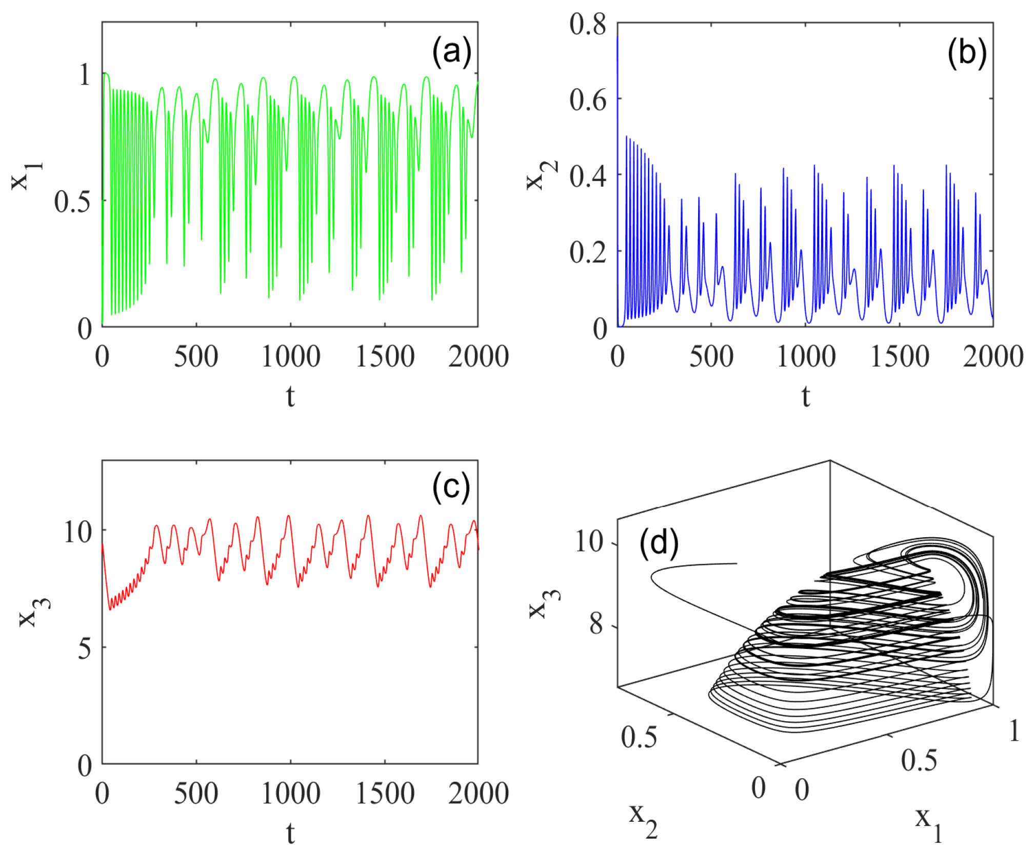
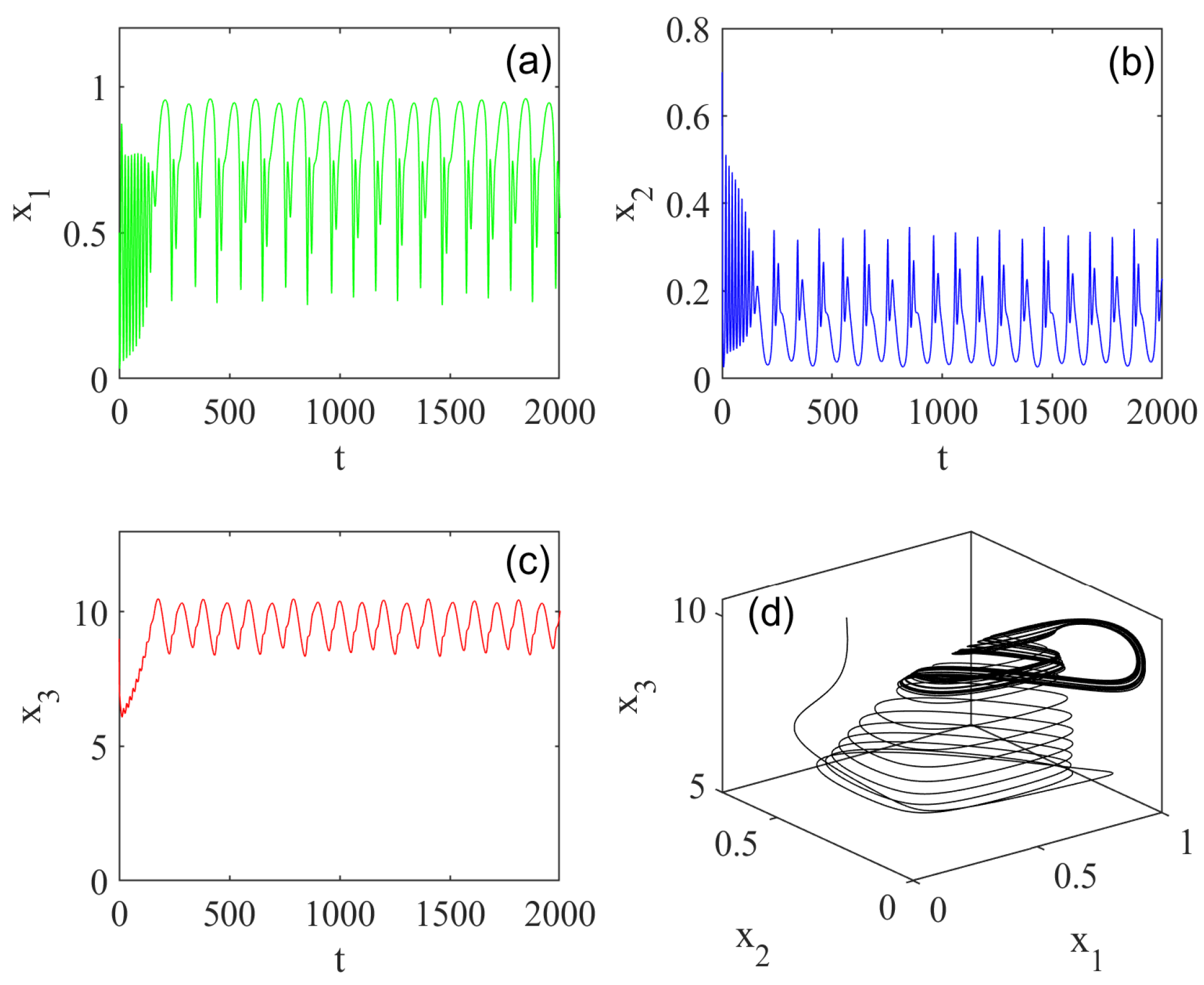
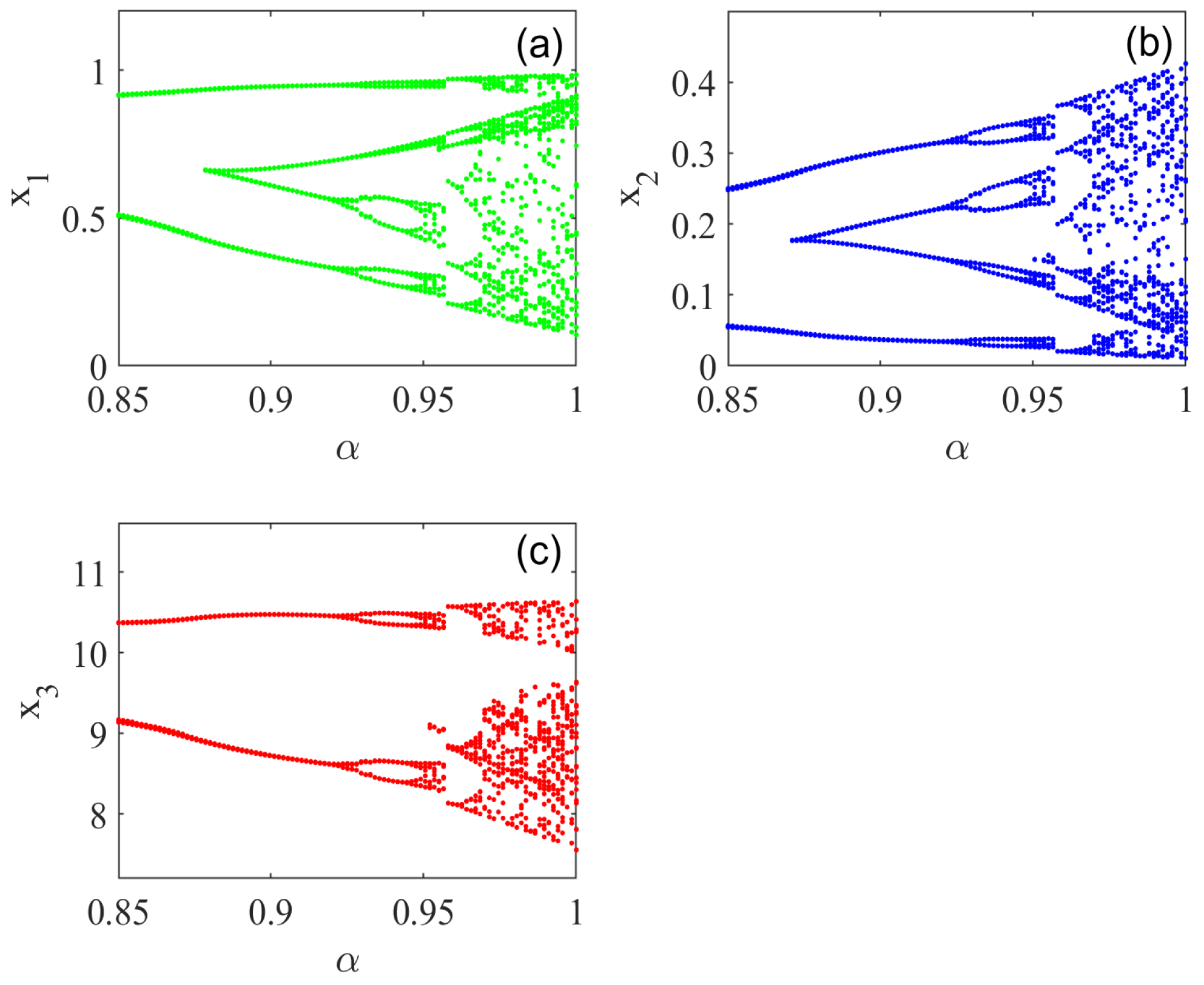
5.1. Effect of Fractional Order

To showcase the effect of the fractional-order quality of Model (3), the different phase portraits are portrayed in Figure 2. First, for $\alpha =0.95,0.9$, Model (3) shows chaotic dynamics; on further decreases, when $\alpha =0.85$, the model exhibits periodic dynamics, and for $\alpha =0.8$, Model (3) reaches an asymptotically stable state. It is shown that Model (3) changes to regular from irregular dynamics when decreasing the order parameter. Thus, Model (3) has more sensitivity in the order parameter and greatly influences the considered model’s dynamics. In [11], the authors showed that the integer-order model undergoes periodic doubling and reverse periodic doubling on increasing the parameter $r_1$. To give a comparison with the fractional-order model, we display the effect of parameter $r_1$ with $\alpha =0.95$ in the one-parameter bifurcation diagram in Figure 3. It is verified that the model is less chaotic and undergoes Hopf bifurcation into higher periodic dynamics. Similarly, higher periodic orbits are shown in the one-parameter bifurcation diagram by varying $r_1\in (2,5)$ in Figure 4.

5.2. Effect of Habitat Complexity

Then, by adjusting $\sigma \in [0,1]$ and setting $\alpha =0.95$, $\gamma =0$, and $\rho =0$, we confirm the impact of habitat complexity. In Figure 5, we showed the one-parameter bifurcation to demonstrate the full dynamics of Model (3). It can be described that when $\sigma$ increases, the model experiences Hopf bifurcation by reverse period doubling. The model simplifies to a periodic orbit for $\sigma =0.5$ and includes higher-order periodic dynamics at the lower value of $\sigma =0.1$. The asymptotically stable state for $\sigma \approx 0.85$ is then reached. Additionally, at larger levels, the habitat complexity $\sigma =0.95$ in the basal prey leads to the extinction of $x_3$ due to considerable changes in the size of the top predator population. The model’s habitat complexity in (3) may be a major factor in the survival or extinction of the relevant populations.

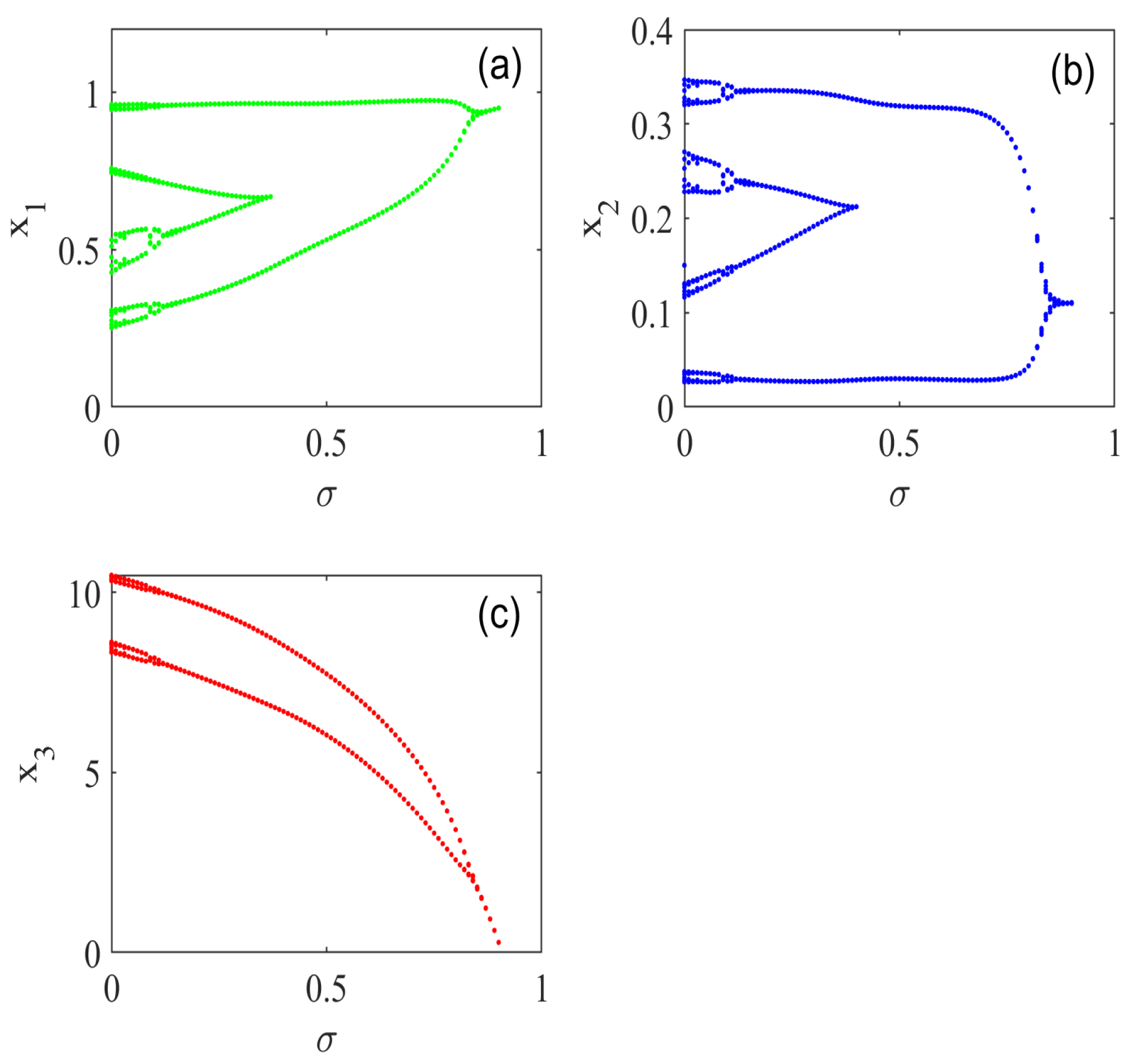
5.3. Effect of Basal Prey Vigilance

Further, it is important to verify the effect of basal prey vigilance in the considered model. For this, we vary $\rho \in [0,0.07]$, fixing $\alpha =0.95$; all other parameters are the same as in (17). Model (3) shows a similar kind of dynamics as for habitat complexity $\sigma$. Model (3) undergoes Hopf bifurcation via reverse period doubling on increasing the prey’s vigilance parameter. For the larger value of $\rho =0.07$, the top predator’s size eventually leads to extinction. Similar results for the integer model in [11] showed the extinction of one or more species for a higher value of basal prey vigilance. The changes in the density of the population by varying the prey vigilance parameter are depicted in Figure 6.

5.4. Effect of Middle Predator Vigilance

Verifying the impact of middle predator vigilance in the model under consideration is also crucial. All other parameters are the same as in (17), and we change $\gamma \in [0,0.8]$, while fixing $\alpha =0.95$. The dynamics of Model (3) are comparable to those of habitat complexity $\sigma$. As the prey’s vigilance parameter increases, Model (3) experiences Hopf bifurcation by reverse period doubling. When $\gamma =0.8$ is greater, the magnitude of the top predator finally causes extinction. According to similar findings for the integer model in [11], a greater value of basal prey vigilance resulted in the extinction of one or more species. Figure 7 illustrates how the prey vigilance parameter affects population densities.

Remark 1.

Since the predator population may disappear from the ecosystem for a relatively high degree of vigilance due to decreased prey availability, studying the vigilance effect is one of the more intriguing problems facing population models. In [15], for example, the relevant tri-tropic food chain system incorporates the vigilant behaviors of the middle predator and the basal prey. They came to the conclusion that the degree of vigilance exhibited by populations of small predators and prey may be a significant factor in the ability of the populations to survive or go extinct. Its equilibrium density grew when the intermediate predators’ level of vigilance went from low to high, reaching a particular threshold. This demonstrates that the total advantage of the middle predator’s decreased rate of predation by the top predator surpasses the loss resulting from less foraging. The model in [11] was compared to the food chain model examined by [15], taking into account both predators feeding on prey in the form of Holling type II. The food chain system can establish long-term coexistence by regulating chaotic oscillations caused by basal prey vigilance. However, greater vigilance among base prey is undesirable to the system since it results in the extinction of one or more species. Thus, in a three-species food chain model, trophic cascades begin when prey demonstrate awareness through behavioral changes in response to the fear of predation threats. In [12], a basic discrete-time predator–prey model was explored, assuming that vigilance affects both prey growth rate and predation rate.

Remark 2.

The fractional-order food chain model used in this study incorporates the impacts of vigilance and habitat complexity. The model examined in [11] is a simplified version of the model as an integer-order model with no habitat complexity. By taking $\alpha =1$ into consideration, we demonstrated the chaotic character of the integer-order model. The model was subsequently reduced from chaotic to stable and periodic dynamics by decreasing the derivative order, while accounting for the Caputo-type fractional order. The introduction of habitat complexity helped to stabilize the model by improving its capacity to attain stable dynamics. Intermediate predators and base prey both show attentiveness. In recent years, Caputo-type fractional systems have attracted a lot of attention and applications [25,26,27,45]. We found that changes in one species’ level of vigilance have a major effect on the density of all the species. Therefore, in a fractional-order three-species food chain model, trophic cascades begin when prey exhibit vigilance through behavioral changes in response to fears of predation risks. Studying the dynamic complexity of ecosystems will benefit from this. Additionally, this study helps to establish broad conclusions on the coexistence of interacting species and the survival or extinction of populations.

6. Conclusions

In this work, the results of a fractional-order food chain model, which included the impacts of habitat complexity and vigilance, were generalized to predators and prey. We determined the conditions that give rise to the fractional system’s equilibrium. We also deduced requirements for the stability of the positive equilibria. To confirm the feasibility of the results, a few numerical simulations were provided. We found rich dynamical behavior in the fractional-order derivative. Additionally, by adjusting the fractional order $\alpha \in (0,1)$, very intricate dynamics were seen. Our suggested model’s solution was shown to be unstable for integer-order cases, while our system’s solution was shown to be stable for fractional-order derivatives.

If the impact on habitat complexity is more severe, the predator population will decrease. An important goal of ecological research is to understand the connection between predators and prey. There is emerging evidence that habitat complexity reduces predator encounter rates and foraging efficiency. Our proposed model is physiologically realistic as positive events in the first quadrant remain stable and evenly limited throughout time. We used bifurcation analysis to determine the degree of habitat complexity, and the results showed that, regardless of how sensitive the prey population is, a higher degree of habitat complexity increases the likelihood of the predator going extinct and that the carrying capacity of the prey will be the only constant attractor.

As a result, the current work outlines many potential dynamical behaviors of a fractional-order food chain model. Therefore, our research will be useful in understanding how species interact with greater ecological implications. Potential research directions may include extensions of this topic related to the Allee effect in the proposed system and may include more simulation results to demonstrate the dynamics with respect to fractional order.

References

1. Hastings, A.; Powell, T. Chaos in a three-species food chain. Ecology 1991, 72, 896–903. [Google Scholar] [CrossRef]
2. Upadhyay, R.K.; Naji, R.K. Dynamics of a three species food chain model with Crowley–Martin type functional response. Chaos Solitons Fractals 2009, 42, 1337–1346. [Google Scholar] [CrossRef]
3. Jana, D.; Agrawal, R.; Upadhyay, R.K. Top-predator interference and gestation delay as determinants of the dynamics of a realistic model food chain. Chaos Solitons Fractals 2014, 69, 50–63. [Google Scholar] [CrossRef]
4. Vinoth, S.; Sivasamy, R.; Sathiyanathan, K.; Rajchakit, G.; Hammachukiattikul, P.; Vadivel, R.; Gunasekaran, N. Dynamical analysis of a delayed food chain model with additive Allee effect. Adv. Differ. Equ. 2021, 2021, 54. [Google Scholar] [CrossRef]
5. Holling, C.S. The components of predation as revealed by a study of small-mammal predation of the European Pine Sawfly1. Can. Entomol. 1959, 91, 293–320. [Google Scholar] [CrossRef]
6. Holling, C.S. Some characteristics of simple types of predation and parasitism1. Can. Entomol. 1959, 91, 385–398. [Google Scholar] [CrossRef]
7. Murray, J.D. Mathematical Biology: I. An Introduction; Springer Science & Business Media: Berlin/Heidelberg, Germany, 2007; Volume 17. [Google Scholar]
8. Canion, C.R.; Heck, K.L., Jr. Effect of habitat complexity on predation success: Re-evaluating the current paradigm in seagrass beds. Mar. Ecol. Prog. Ser. 2009, 393, 37–46. [Google Scholar] [CrossRef]
9. Scharf, F.S.; Manderson, J.P.; Fabrizio, M.C. The effects of seafloor habitat complexity on survival of juvenile fishes: Species-specific interactions with structural refuge. J. Exp. Mar. Biol. Ecol. 2006, 335, 167–176. [Google Scholar] [CrossRef]
10. Johnson, M.P.; Frost, N.J.; Mosley, M.W.; Roberts, M.F.; Hawkins, S.J. The area-independent effects of habitat complexity on biodiversity vary between regions. Ecol. Lett. 2003, 6, 126–132. [Google Scholar] [CrossRef]
11. Hossain, M.; Kumbhakar, R.; Pal, N. Dynamics in the biparametric spaces of a three-species food chain model with vigilance. Chaos Solitons Fractals 2022, 162, 112438. [Google Scholar] [CrossRef]
12. Hossain, M.; Garai, S.; Jafari, S.; Pal, N. Bifurcation, chaos, multistability, and organized structures in a predator–prey model with vigilance. Chaos Interdiscip. J. Nonlinear Sci. 2022, 32, 063139. [Google Scholar] [CrossRef]
13. Creel, S. The control of risk hypothesis: Reactive vs. proactive antipredator responses and stress-mediated vs. food-mediated costs of response. Ecol. Lett. 2018, 21, 947–956. [Google Scholar] [CrossRef] [PubMed]
14. Hunter, L.T.; Skinner, J.D. Vigilance behaviour in African ungulates: The role of predation pressure. Behaviour 1998, 135, 195–211. [Google Scholar] [CrossRef]
15. Hossain, M.; Garai, S.; Karmakar, S.; Pal, N.; Chattopadhyay, J. Impact of vigilance on the density variations in a food chain model. Ecol. Complex. 2022, 50, 100996. [Google Scholar] [CrossRef]
16. Ramasamy, S.; Banjerdpongchai, D.; Park, P. Stability and Hopf-bifurcation analysis of diffusive Leslie–Gower prey–predator model with the Allee effect and carry-over effects. Math. Comput. Simul. 2025, 227, 19–40. [Google Scholar] [CrossRef]
17. Petráš, I. Fractional-Order Nonlinear Systems: Modeling, Analysis and Simulation; Springer Science & Business Media: Berlin/Heidelberg, Germany, 2011. [Google Scholar]
18. Podlubny, I. Fractional Differential Equations: An Introduction to Fractional Derivatives, Fractional Differential Equations, to Methods of Their Solution and Some of Their Applications; Elsevier: Amsterdam, The Netherlands, 1998. [Google Scholar]
19. Ionescu, C.; Lopes, A.; Copot, D.; Machado, J.T.; Bates, J.H. The role of fractional calculus in modeling biological phenomena: A review. Commun. Nonlinear Sci. Numer. Simul. 2017, 51, 141–159. [Google Scholar] [CrossRef]
20. Du, M.; Wang, Z.; Hu, H. Measuring memory with the order of fractional derivative. Sci. Rep. 2013, 3, 3431. [Google Scholar] [CrossRef] [PubMed]
21. Panigoro, H.S.; Suryanto, A.; Kusumawinahyu, W.M.; Darti, I. A Rosenzweig–MacArthur model with continuous threshold harvesting in predator involving fractional derivatives with power law and mittag–leffler kernel. Axioms 2020, 9, 122. [Google Scholar] [CrossRef]
22. Veeresha, P.; Prakasha, D.; Singh, J.; Khan, I.; Kumar, D. Analytical approach for fractional extended Fisher–Kolmogorov equation with Mittag-Leffler kernel. Adv. Differ. Equ. 2020, 2020, 174. [Google Scholar] [CrossRef]
23. Muhammad Altaf, K.; Atangana, A. Dynamics of Ebola disease in the framework of different fractional derivatives. Entropy 2019, 21, 303. [Google Scholar] [CrossRef] [PubMed]
24. Almeida, R.; Bastos, N.R.; Monteiro, M.T.T. Modeling some real phenomena by fractional differential equations. Math. Methods Appl. Sci. 2016, 39, 4846–4855. [Google Scholar] [CrossRef]
25. Padder, A.; Almutairi, L.; Qureshi, S.; Soomro, A.; Afroz, A.; Hincal, E.; Tassaddiq, A. Dynamical analysis of generalized tumor model with Caputo fractional-order derivative. Fractal Fract. 2023, 7, 258. [Google Scholar] [CrossRef]
26. Vadivel, R.; Hammachukiattikul, P.; Vinoth, S.; Chaisena, K.; Gunasekaran, N. An extended dissipative analysis of fractional-order fuzzy networked control systems. Fractal Fract. 2022, 6, 591. [Google Scholar] [CrossRef]
27. Olayiwola, M.O.; Alaje, A.I.; Olarewaju, A.Y.; Adedokun, K.A. A Caputo fractional order epidemic model for evaluating the effectiveness of high-risk quarantine and vaccination strategies on the spread of COVID-19. Healthc. Anal. 2023, 3, 100179. [Google Scholar] [CrossRef]
28. Mondal, S.; Biswas, M.; Bairagi, N. Local and global dynamics of a fractional-order predator–prey system with habitat complexity and the corresponding discretized fractional-order system. J. Appl. Math. Comput. 2020, 63, 311–340. [Google Scholar] [CrossRef]
29. Panja, P. Stability and dynamics of a fractional-order three-species predator–prey model. Theory Biosci. 2019, 138, 251–259. [Google Scholar] [CrossRef] [PubMed]
30. Panja, P. Dynamics of a fractional order predator-prey model with intraguild predation. Int. J. Model. Simul. 2019, 39, 256–268. [Google Scholar] [CrossRef]
31. Garrappa, R. Short Tutorial: Solving Fractional Differential Equations by Matlab Codes; Department of Mathematics, University of Bari: Bari, Italy, 2014. [Google Scholar]
32. Caputo, M. Linear models of dissipation whose Q is almost frequency independent—II. Geophys. J. Int. 1967, 13, 529–539. [Google Scholar] [CrossRef]
33. Diethelm, K.; Ford, N. The Analysis of Fractional Differential Equations; Lecture Notes in Mathematics; Springer: Berlin/Heidelberg, Germany, 2010. [Google Scholar]
34. Matignon, D. Stability results for fractional differential equations with applications to control processing. In Proceedings of the Computational Engineering in Systems Applications, Lille, France, 9–12 July 1996; Volume 2, pp. 963–968. [Google Scholar]
35. Li, H.L.; Zhang, L.; Hu, C.; Jiang, Y.L.; Teng, Z. Dynamical analysis of a fractional-order predator-prey model incorporating a prey refuge. J. Appl. Math. Comput. 2017, 54, 435–449. [Google Scholar] [CrossRef]
36. Choi, S.; Kang, B.; Koo, N. Stability for fractional differential equations. Proc. Jangjeon Math. Soc. 2013, 16, 165–174. [Google Scholar]
37. Choi, S.K.; Kang, B.; Koo, N. Stability for Caputo fractional differential systems. Abstr. Appl. Anal. 2014, 2014, 631419. [Google Scholar] [CrossRef]
38. Li, C.; Ma, Y. Fractional dynamical system and its linearization theorem. Nonlinear Dyn. 2013, 71, 621–633. [Google Scholar] [CrossRef]
39. Tavazoei, M.S.; Haeri, M.; Attari, M.; Bolouki, S.; Siami, M. More details on analysis of fractional-order Van der Pol oscillator. J. Vib. Control 2009, 15, 803–819. [Google Scholar] [CrossRef]
40. Tavazoei, M.S.; Haeri, M. A proof for non existence of periodic solutions in time invariant fractional order systems. Automatica 2009, 45, 1886–1890. [Google Scholar] [CrossRef]
41. Tavazoei, M.S. A note on fractional-order derivatives of periodic functions. Automatica 2010, 46, 945–948. [Google Scholar] [CrossRef]
42. Abdelouahab, M.S.; Hamri, N.E.; Wang, J. Hopf bifurcation and chaos in fractional-order modified hybrid optical system. Nonlinear Dyn. 2012, 69, 275–284. [Google Scholar] [CrossRef]
43. Yazdani, M.; Salarieh, H. On the existence of periodic solutions in time-invariant fractional order systems. Automatica 2011, 47, 1834–1837. [Google Scholar] [CrossRef]
44. Danca, M.F. Matlab code for Lyapunov exponents of fractional-order systems, part ii: The noncommensurate case. Int. J. Bifurc. Chaos 2021, 31, 2150187. [Google Scholar] [CrossRef]
45. E. Alsubaie, N.; EL Guma, F.; Boulehmi, K.; Al-kuleab, N.; A. Abdoon, M. Improving influenza epidemiological models under Caputo fractional-order calculus. Symmetry 2024, 16, 929. [Google Scholar] [CrossRef]
Figure 1. Chaotic time series (ac) and phase portrait (d) for Model (3) with α = 1 . All other essential parameters are given in (17).
Fractalfract 09 00045 g001
Figure 2. Different phase portraits for Model (3) for different values of α , for α = 0.95 , which is chaotic in (a), for α = 0.9 , which is also chaotic in (b), for α = 0.85 , which shows a periodic orbit in (c), and for α = 0.8 , which is asymptotically stable state in (d).
Fractalfract 09 00045 g002
Figure 3. One-parameter bifurcation diagram for Model (3) as fractional order α varies within range ( 0.85 , 1 ) . Diagram illustrates transition in system dynamics, highlighting changes in periodic from chaotic dynamics as α approaches 0.85. (a), (b), and (c) are the sizes of the populations x 1 , x 2 , and x 3 .
Fractalfract 09 00045 g003
Figure 4. One-parameter bifurcation diagram for Model (3) as parameter r 1 varies within range ( 2 , 5 ) . Diagram depicts evolution of system’s dynamic behavior, showcasing changes in stability and bifurcation points as r 1 increases. (a), (b), and (c) are the sizes of the populations x 1 , x 2 , and x 3 .
Fractalfract 09 00045 g004
Figure 5. One-parameter bifurcation diagram for Model (3) by varying σ ( 0 , 1 ) . Results demonstrate that larger values of σ lead to more stable dynamics in system. (a), (b), and (c) are the sizes of the populations x 1 , x 2 , and x 3 .
Fractalfract 09 00045 g005
Figure 6. One-parameter bifurcation for Model (3) by varying ρ ( 0 , 0.8 ) . The results indicate that increasing ρ enhances the stability of the model, with larger values of ρ leading to greater stability.(a), (b), and (c) are the sizes of the populations x 1 , x 2 , and x 3 .
Fractalfract 09 00045 g006
Figure 7. One-parameter bifurcation for Model (3) by varying γ ( 0 , 0.07 ) . The results indicate that increasing γ enhances the stability of the model, with larger values of γ leading to stable dynamics. (a), (b), and (c) are the sizes of the populations x 1 , x 2 , and x 3 .
Fractalfract 09 00045 g007
Disclaimer/Publisher’s Note: The statements, opinions and data contained in all publications are solely those of the individual author(s) and contributor(s) and not of MDPI and/or the editor(s). MDPI and/or the editor(s) disclaim responsibility for any injury to people or property resulting from any ideas, methods, instructions or products referred to in the content.