Article

Nonlinear Fractional Evolution Control Modeling via Power Non-Local Kernels: A Generalization of Caputo–Fabrizio, Atangana–Baleanu, and Hattaf Derivatives

1
Department of Mathematics, College of Science, University of Ha’il, Ha’il 55473, Saudi Arabia
2
Department of Artificial Intelligence, College of Computer and Information Technology, Al-Razi University, Sana’a 12544, Yemen
3
Department of Mathematics, College of Science, Qassim University, Buraydah 51452, Saudi Arabia
4
Department of Mathematics, College of Science and Humanities in Al-Kharj, Prince Sattam Bin Abdulaziz University, Al-Kharj 11942, Saudi Arabia
5
Department of Mathematics, Faculty of Science, Islamic University of Madinah, Madinah 42351, Saudi Arabia
6
Department of Mathematics, Faculty of Science, University of Tabuk, P.O. Box 741, Tabuk 71491, Saudi Arabia
*
Authors to whom correspondence should be addressed.
Fractal Fract. 2025, 9(2), 104; https://doi.org/10.3390/fractalfract9020104
Submission received: 18 December 2024 / Revised: 3 February 2025 / Accepted: 5 February 2025 / Published: 8 February 2025

Abstract

:
This paper presents a novel framework for modeling nonlinear fractional evolution control systems. This framework utilizes a power non-local fractional derivative (PFD), which is a generalized fractional derivative that unifies several well-known derivatives, including Caputo–Fabrizio, Atangana–Baleanu, and generalized Hattaf derivatives, as special cases. It uniquely features a tunable power parameter “p”, providing enhanced control over the representation of memory effects compared to traditional derivatives with fixed kernels. Utilizing the fixed-point theory, we rigorously establish the existence and uniqueness of solutions for these systems under appropriate conditions. Furthermore, we prove the Hyers–Ulam stability of the system, demonstrating its robustness against small perturbations. We complement this framework with a practical numerical scheme based on Lagrange interpolation polynomials, enabling efficient computation of solutions. Examples illustrating the model’s applicability, including symmetric cases, are supported by graphical representations to highlight the approach’s versatility. These findings address a significant gap in the literature and pave the way for further research in fractional calculus and its diverse applications.

1. Introduction

The concept of fractional calculus (FC) [1,2,3] originated in a 1695 correspondence between l’Hôpital and Leibniz, who first explored the idea of derivatives of non-integer order (such as 1/2). Despite early contributions from mathematicians like Euler, Fourier, Abel, and Liouville, the field’s progress was initially hindered by the lack of a clear geometric interpretation analogous to that of the derivative in classical calculus [4,5,6]. Over time, definitions evolved from integral representations (Fourier) and exponential function differentiation (Liouville) to series-based approaches like that of Grünwald–Letnikov. Subsequently, numerous fractional derivatives have been proposed, including those with both singular and non-singular kernels [7,8,9,10]. Examples include Jumarie’s fractional derivative, He’s fractional derivative, the Grünwald–Letnikov derivative, Sonin–Letnikov derivative, Liouville derivative, Caputo derivative, Hadamard derivative, Marchaud derivative, Riesz derivative, Miller–Ross derivative, Weyl derivative, Erdélyi–Kober derivative, Coimbra derivative, Katugampola derivative, Hilfer derivative, Davidson derivative, Chen derivative, Caputo Fabrizio derivative, and Atangana–Baleanu derivative [10,11,12,13].
Fractional evolution equations are increasingly used in science and engineering due to their capacity to accurately model complex phenomena not adequately described by traditional integer-order formulations. Specifically, these equations effectively capture systems exhibiting anomalous diffusion, memory effects, and non-local interactions, which are prevalent in diverse domains such as viscoelasticity, hydrology, finance, and biology [14,15,16,17]. Employing fractional-order operators allows for the development of more accurate and realistic models, ultimately leading to improved predictive capabilities and innovative solutions. Consequently, significant research has focused on the fundamental qualitative behavior of solutions to fractional evolution equations. This includes analyzing existence and uniqueness criteria, exploring stability concepts (e.g., Ulam–Hyers stability), and establishing conditions for controllability. These investigations have led to substantial progress in the theoretical foundation of this area. For example, Kavitha et al. [18] have studied the existence of solutions for Hilfer fractional neutral evolution equations with infinite delay, Raja et al. [19] explored the existence and controllability of fractional evolution inclusions, Saber et al. [20] investigated a Fractional Evolution Control Model using W-Piecewise hybrid derivatives, and Almalahi et al. [21] analyzed second-order nonlinear fractional differential evolution equations using a generalized Atangana–Baleanu–Caputo (ABC) operator.
A key advancement in fractional calculus has been the development of non-local fractional derivatives using non-singular kernels. Unlike traditional fractional derivatives with singular kernels, these derivatives avoid singularities at the origin, improving their mathematical properties and their consistency with experimental observations. Notable examples of these derivatives include the Atangana–Baleanu [22], Caputo–Fabrizio [23], Hattaf [24], and weighted Atangana–Baleanu [25] derivatives, each with unique features for various modeling applications [26,27,28,29,30].
Building upon these developments, a novel power fractional derivative (PFD) was recently introduced [31], distinguished by its incorporation of a crucial “power” parameter, *p*, in the generalized power Mittag–Leffler (PML) function. This parameter provides flexibility, enabling researchers to fine-tune the fractional derivative for specific system dynamics. The PFD represents a significant generalization of existing non-local fractional derivatives with non-singular kernels, offering new possibilities for studying nonlinear wave equations such as the nonlinear Schrödinger (NLS) and modified Korteweg–de Vries (mKdV) models. By varying the value of p, the PFD can be adapted to different memory effects and complex dynamics, offering a more nuanced and accurate representation of real-world processes. Prior research on PFDs [31] has focused on their basic properties and applications to linear fractional differential equations. Recently, Zitane et al. [32] investigated existence, uniqueness, and numerical approximations for a class of fractional differential equations using power non-local and non-singular kernels. However, the analysis of nonlinear fractional differential equations incorporating PFDs remains a relatively unexplored topic.
Motivated by the significance of evolution control equations and the benefits of employing power non-local fractional operators, this study investigates a class of nonlinear Fractional Evolution Control Models utilizing power non-local kernels. Several special symmetric cases are explored, and we aim to establish fundamental criteria for qualitative behaviors, including existence, uniqueness, and stability, for the nonlinear Fractional Evolution Control Models (PFECMs) using power non-local kernels, as described by the following equation:
D ς , w β , δ , p a         PC y ( ς ) Z ς , y ς = Ω y ( ς ) + K ς , y ς , ς J : = a , b y ( a ) = y a ,
where D ς , w β , δ , p a         PC is the PFD of order β 0 , 1 , in the Caputo sense, with respect to weight function w, min δ , p > 0 , and the function y H 1 a , b , and Ω generates an analytic semigroup of bounded linear operators. Z , K : J × R R are continuous and satisfy some conditions to be described later.
The PFECM (1) generalizes many models depending on the parameters β , δ , e , and weight function w ( ς ) . The symmetric cases of PFECM (1) are given as follows:
  • If p = e , then the PFECM (1) reduces to the weighted generalized Hattaf fractional model:
    D ς , w β , δ , e a         PC y ( ς ) Z ς , y ς = Ω y ( ς ) + K ς , y ς , y ( a ) = y a .
  • If δ = β , p = e and w ς = 1 , then the model (1) reduces to the Atangana–Baleanu fractional model:
    D ς , 1 β , β , e a         PC y ( ς ) Z ς , y ς = Ω y ( ς ) + K ς , y ς , y ( a ) = y a .
  • If δ = β , and p = e , then the model (1) reduces to another form of the Atangana–Baleanu fractional model:
    D ς , w β , β , e a         PC y ( ς ) Z ς , y ς = Ω y ( ς ) + K ς , y ς , y ( a ) = y a .
  • If δ = 1 , p = e and w ς = 1 , then the model (1) reduces to the Caputo–Fabrizio fractional model:
    D ς , 1 β , 1 , e a         PC y ( ς ) Z ς , y ς = Ω y ( ς ) + K ς , y ς , y ( a ) = y a .
The physical relevance of our fractional model lies in its ability to capture phenomena characterized by memory and non-local interactions. Unlike traditional integer-order derivatives, fractional derivatives inherently incorporate the influence of a system’s past states on its present behavior. This is crucial for describing processes in viscoelasticity, anomalous diffusion, and porous media, where the system’s history significantly affects its dynamics. The power parameter ‘p’ in our proposed PFD allows us to fine-tune the degree of memory influence, offering a refined way to represent diverse physical systems. By using the PFD, we move beyond traditional models to a framework capable of modeling complex behaviors, offering a physically motivated approach to analyzing systems with intricate temporal dependencies.
By addressing both theoretical aspects, such as existence and uniqueness, and the practical need for numerical solutions, this research significantly advances the field of fractional calculus and enables wider application of PFDs in modeling complex real-world phenomena. This is especially important given the increasing recognition of the PFD’s capacity for capturing intricate dynamics in systems with memory effects.

1.1. Contribution and Novelty of This Work

This research introduces a novel framework for modeling nonlinear fractional evolution control systems using power non-local kernels. The core innovation lies in the PFD, a generalized fractional derivative that incorporates a tunable power parameter, *p*, enabling fine-grained control over the memory effects captured by the model. The PFD generalizes well-known fractional derivatives, including Caputo–Fabrizio, Atangana–Baleanu, and Hattaf derivatives, making it a versatile tool for modeling complex systems.
In this work, we rigorously establish the existence and uniqueness of solutions for the PFECM involving the PFD and demonstrate their Hyers–Ulam stability, addressing a crucial gap in the understanding of these models. We develop a numerical scheme based on Lagrange interpolation polynomials to solve the PFECM and illustrate its application through examples, including symmetric cases (Caputo–Fabrizio, Atangana–Baleanu, and Hattaf derivatives). Graphical comparisons are provided to demonstrate the versatility of the approach. This combination of a new generalized fractional derivative, rigorous theoretical analysis, and practical numerical implementation, constitutes a significant advancement in fractional calculus and its application to complex systems.

1.2. Advantages of a Power Non-Local Fractional Operator

Traditional fractional derivatives, such as Riemann–Liouville and Caputo, rely on singular kernels, which can hinder theoretical analysis, numerical computations, and physical interpretation. While non-singular kernel derivatives like Caputo–Fabrizio and Atangana–Baleanu address some of these issues, their fixed kernel structures still lack the flexibility needed to fully capture the diverse memory effects observed in real-world phenomena.
The PFD overcomes these limitations by using non-singular kernels and introducing a tunable power parameter, *p*. This parameter enables precise control over the derivative’s behavior, allowing researchers to tailor the PFD to specific system dynamics and capture a wider spectrum of memory effects. By generalizing existing non-singular kernel derivatives, the PFD provides a unified framework that enhances both theoretical and practical applications of fractional calculus.
Unlike Jumarie’s and He’s fractional derivatives [33,34], which are defined locally using approximations at a single point, the PFD is defined non-locally over an interval using the generalized Mittag–Leffler function, providing a clear mathematical representation for the memory effect. Furthermore, Jumarie’s and He’s derivatives have limitations when fractional orders approach zero or one, whereas the PFD, based on an integral representation, avoids these limitations. The PFD offers a more general framework that includes several well-established non-singular kernel derivatives as special cases, while Jumarie’s and He’s fractional derivatives do not provide this level of generalization [35].

2. Basic Concepts

To establish a foundation for our subsequent analysis, this section introduces essential concepts related to fractional operators characterized by power non-local and non-singular kernels [31].
Definition 1 
([31]). Let β 0 , 1 , with δ , p > 0 , and y H 1 a , b , where H 1 a , b is Sobolev space. The PFD of order β, in the Caputo sense, of a function y with respect to the weight function w , 0 < w C 1 a , b , is defined by
D ς , w β , δ , p a         PC y ( ς ) = PC ( β ) 1 β 1 w ( ς ) a ς E δ , 1 p β 1 β ς s δ w y s d s ,
where,
  • E δ , 1 p represents the PML function given by
    E δ , l p s = n = 0 + s ln p n Γ k n + l , s C , a n d   k , l , p > 0 .
  • PC ( β ) represents a normalization positive function obeying PC ( 0 ) = PC ( 1 ) = 1 .
According to Theorem 1 of [31], the PML function E δ , l p s is locally uniformly convergent for any s C ; see Theorem 1 of [31].
Remark 1. 
The PFD in the Caputo sense, as given by Definition 1, generalizes many fractional derivatives found in the literature, as follows:
(1) If w ( ς ) = 1 , p = e , δ = 1 , then Definition 1 reduces to the Caputo–Fabrizio fractional derivative, given by
D ς , 1 β , 1 , e a         PC y ( ς ) = PC ( β ) 1 β a ς exp β 1 β ς s y s d s .
(2) If w ( ς ) = 1 , p = e , β = δ , then Definition 1 reduces to the Atangana–Baleanu fractional derivative, given by
D ς , 1 β , β , e a         PC y ( ς ) = PC ( β ) 1 β a ς E β , 1 e β 1 β ς s β y s d s .
(3) If p = e , β = δ , then Definition 1 reduces to the weighted Atangana–Baleanu fractional derivative, given by
D ς , w β , β , e a         PC y ( ς ) = PC ( β ) 1 β 1 w ( ς ) a ς E β , 1 e β 1 β ς s β w y s d s .
(4) If p = e , then Definition 1 reduces to the weighted generalized Hattaf fractional derivative, given by
D ς , w β , δ , e a         PC y ( ς ) = PC ( β ) 1 β 1 w ( ς ) a ς E δ , 1 e β 1 β ς s δ w y s d s .
Definition 2 
([31]). The Power Fractional Integral (PFI) of order β, for a function y with respect to the weight function w , (where 0 < w C 1 a , b ), is defined by
I ς , w β , δ , p a         PC y ( ς ) = 1 β PC ( β ) y ( ς ) + ln p β PC ( β ) RL I a , w δ y ( ς ) ,
where the following apply:
  • I a , w δ RL y ( ς ) denotes the standard weighted Riemann–Liouville fractional integral of order δ given by
    I a , w δ RL y ( ς ) = 1 Γ ( δ ) 1 w ς a ς ς s δ 1 w y s d s .
Remark 2. 
Formula (6) can be expressed as follows:
D ς , w β , δ , p a         PC y ( ς ) = PC ( β ) 1 β n = 0 + β 1 β ς s δ n I a , w δ n + 1 RL w y w ς ,
where the series converges locally and uniformly in ς .
Theorem 1 
([36]). Let β 0 , 1 , with δ , p > 0 , and y H 1 a , b . Then, the PFD and PFI are commutative operators as follows:
(i)
D ς , w β , δ , p a         PC I ς , w β , δ , p a         PC y ( ς ) = y ( ς ) w y a w ( ς ) ;
(ii)
I ς , w β , δ , p a         PC D ς , w β , δ , p a         PC y ( ς ) = y ( ς ) w y a w ( ς ) .
If we set p = e , we obtain the results corresponding to the generalized Hattaf fractional operators [37].
Remark 3. 
The PFD and PFI satisfy the Newton–Leibniz formula:
D ς , w β , δ , p a         PC I ς , w β , δ , p a         PC y ( ς ) = I ς , w β , δ , p a         PC D ς , w β , δ , p a         PC y ( ς ) = y ς y a .
Lemma 1 
([36]). Let K : 0 , 1 × R R be a continuous nonlinear function such that K a , y a = 0 . Then, the function y C a , b is a solution of the following problem:
D ς , w β , δ , p a         PC y ς = K ς , y ς , y 0 = y a R ,
if and only if y satisfies the following integral equation:
y ς = w a w ς y a + I ς , w β , δ , p a         PC K ς , y ς .
Definition 3. 
Assume V : N Q Q is a bounded continuous operator. If for all u , u ^ N , we have
V ( u ) V ( u ^ ) Υ u u ^ , Y > 0 .
Then, V is Lipschitz operator with Lipschitz constant Y. Moreover, if Y < 1 , then V is a strict contraction operator.
Proposition 1. 
If V : N Q is compact, then V satisfies the property of being Y–Lipschitz with a constant equal to 0.
Lemma 2. 
According to Lemma 1, the solution to model (1) is given by
y ς = w a w ς y a + Z ς , y ς + I ς , w β , δ , p a         PC Ω y ( ς ) + K ς , y ς .

2.1. Hypothesis

In the forthcoming analysis, we impose the following assumptions to study the existence, uniqueness, and stability of solutions:
Hypothesis 1. 
H 1 For continuous functions K and Z , there exist constants L K , L Z > 0 such that
K ς , y ( ς ) K ς , y ^ ( ς ) L K y ( ς ) y ^ ( ς ) , f o r   ς J ,
and
Z ς , y ς Z ς , y ^ ς L Z y ( ς ) y ^ ( ς ) , f o r   ς J .
Hypothesis 2. 
H 2 The functions K , Z are continuous, and there exist constants λ K , η K > 0 , and λ Z , η Z such that
K ς , y ( ς ) λ K + y ( ς ) η K , f o r   ς J ,
and
Z ς , y ς λ Z + y ( ς ) η Z , f o r   ς J .
Hypothesis 3. 
H 3 Let Ω > 0 . Then, we have
Ω y ( ς ) Ω y ( ς ) ,

2.2. Notations

To discuss the qualitative behavior of solutions using the fixed-point approach, we define an operator V : Q Q by
V y ( ς ) = w a w ς y a + Z ς , y ς + I ς , w β , δ , p a         PC Ω y ( ς ) + K ς , y ς .
The model given by Equation (1) possesses a solution precisely when the operator V has fixed points. To prepare for our analysis, we introduce the following notations:
O = 1 β PC ( β ) + ln p β PC ( β ) b a δ Γ δ + 1 , Υ = L Z + Ω + L K O .

3. Qualitative Behavior of the Fractional Control Evolution Model (1)

Theorem 2. 
(Y-Lipschitz) Under assumptions ( H 1 H 3 ), the operator V is Y-Lipschitz, where
Υ = L Z + Ω + L K 1 β PC ( β ) + ln p β PC ( β ) b a δ Γ δ + 1 < 1 .
Proof. 
Let y , y ^ Q . Then, for ς a , b , we have
V y ( ς ) V y ^ ( ς ) = Z ς , y ς Z ς , y ^ ς + a PC I ς , w β , δ , p Ω y ( ς ) Ω y ^ ( ς ) + a PC I ς , w β , δ , p K ς , y ς K ς , y ^ ς .
By ( H 1 )and ( H 3 ), we have
V y ( ς ) V y ^ ( ς ) L Z y ( ς ) y ^ ( ς ) + Ω + L K a PC I ς , w β , δ , p y ( ς ) y ^ ( ς ) .
Hence, using Definition 2, one obtains
V y ( ς ) V y ^ ( ς ) L Z y ( ς ) y ^ ( ς ) + Ω + L K × 1 β PC ( β ) y ( ς ) y ^ ( ς ) + ln p β PC ( β ) a RL I ς , w δ y ( ς ) y ^ ( ς ) L Z y ( ς ) y ^ ( ς ) + Ω + L K × Ω + L K y ( ς ) y ^ ( ς ) 1 β PC ( β ) + ln p β PC ( β ) a RL I ς , w δ ( 1 ) ( ς ) L Z + Ω + L K 1 β PC ( β ) + ln p β PC ( β ) a RL I ς , w δ ( 1 ) ( ς ) y ( ς ) y ^ ( ς ) .
Thus, by (8), we have
V y V y ^ L Z + Ω + L K 1 β PC ( β ) + ln p β PC ( β ) a RL I ς , w δ ( 1 ) ( ς ) y y ^ .
Then, by (9), we obtain
V y V y ^ Υ y y ^ .
Thus, V is Υ -Lipschitz. □
Theorem 3. 
(Compactness of V ) The operator V defined by V : Q Q is completely continuous.
Proof. 
Let N be a bounded set defined by N = y Q : y r and let a sequence y n in N , such that y n y as n . This is because Ω and K are continuous. Then, we have
Ω y n ς Ω y ς , as   n , K ς , y n ( ς ) K ς , y ( ς ) , as   n , Z ς , y n ( ς ) Z ς , y ( ς ) , as   n .
Using H 1 , we have
V y n V y L Z y n ( ς ) y ( ς ) + Ω + L K × 1 β PC ( β ) y n ( ς ) y ( ς ) + ln p β PC ( β ) a RL I ς , w δ y n ( ς ) y ( ς ) L Z + Ω + L K O y n y 0 , as   n .
Thus, the operator V is continuous. Let y N . Then, we have
V y ς w a w ς y a + Z ς , y ς + a PC I ς , w β , δ , p Ω y ( ς ) + a PC I ς , w β , δ , p K ς , y ς w a w ς y a + λ Z + y ( ς ) η Z + a PC I ς , w β , δ , p Ω y ( ς ) + a PC I ς , w β , δ , p λ K + y ( ς ) η K w a w ς y a + λ Z + r η Z + Ω + η K r + λ K 1 β PC ( β ) + ln p β PC ( β ) ς a δ Γ δ + 1 .
Thus, by (8), we have
V y w a w * y a + λ Z + r η Z + Ω + η K r + λ K 1 β PC ( β ) + ln p β PC ( β ) ς a δ Γ δ + 1 ,
where w * = min ς a , b w ς . Therefore, V is bounded. To show the equicontinuity property, let a < ς 1 < ς 2 < b , y N . Then, we have
V y ( ς 2 ) V y ( ς 1 ) Z ς 2 , y ς 2 Z ς 1 , y ς 1 + I ς 2 , w β , δ , p a         PC Ω y ( ς 2 ) + K ς 2 , y ς 2 I ς 1 , w β , δ , p a         PC Ω y ( ς 1 ) + K ς 1 , y ς 1 Z ς 2 , y ς 2 Z ς 1 , y ς 1 + I ς 1 , w β , δ , p a         PC Ω y ( ς 2 ) + K ς 2 , y ς 2 Ω y ( ς 1 ) + K ς 1 , y ς 1 + I ς 2 , w β , δ , p ς 1     PC Ω y ( ς 2 ) + K ς 2 , y ς 2 .
Thus, by (H2), we have
V y ( ς 2 ) V y ( ς 1 ) Z ς 2 , y ς 2 Z ς 1 , y ς 1 + Ω r + λ K + r η K ln p β PC ( β ) ς 2 ς 1 δ Γ δ + 1 0   a s   ς 2 ς 1 .
The above argument demonstrates the uniform continuity of V . Therefore, by the Arzela–Ascoli theorem, we infer that V is relatively compact, from which its complete continuity follows. □
Theorem 4. 
(Existence of solution) Under assumptions ( H 1 H 3 ), the PFECM (1) admits a bounded set of solutions, from which the existence of at least one solution can be inferred when
η Z + Ω + η K 1 β PC ( β ) + ln p β PC ( β ) ς a δ Γ δ + 1 < 1 .
Proof. 
As a consequence of Lemma 2, the operator V is shown to be Υ -Lipschitz with Lipschitz constant Υ . A set of solutions the to PFECM (1) can be characterized as follows:
Λ = y Q : 0 , 1 , y = V y ,
which implies that
y = V y w a w ς y a + Z ς , y ς + a PC I ς , w β , δ , p Ω y ( ς ) + a PC I ς , w β , δ , p K ς , y ς .
Thus, by (H2), we have
y w a w * y a + λ Z + η Z + Ω + η K 1 β PC ( β ) + ln p β PC ( β ) ς a δ Γ δ + 1 y + λ K 1 β PC ( β ) + ln p β PC ( β ) ς a δ Γ δ + 1 .
Consider set Λ as unbounded. By dividing both sides of the above inequality by y , we obtain
1 lim y 1 y w a w * y a + λ Z + η Z + Ω + η K 1 β PC ( β ) + ln p β PC ( β ) ς a δ Γ δ + 1 y + λ K 1 β PC ( β ) + ln p β PC ( β ) ς a δ Γ δ + 1 η Z + Ω + η K 1 β PC ( β ) + ln p β PC ( β ) ς a δ Γ δ + 1 < 1 .
The aforementioned contradiction necessitates the boundedness of Λ . Consequently, V possesses at least one fixed point, which corresponds to a solution of the PFECM (1). □
Theorem 5. 
(Uniqueness of solution) Given assumptions (H1, H3), the PFECM (1) has a unique solution, provided that Υ < 1 .
Proof. 
As a consequence of Lemma 2, the operator V defined by (7) is established to be Υ -Lipschitz. It therefore follows, by the contraction mapping principle, that V admits a unique fixed point, representing a unique solution to the PFECM (1). □
Theorems 4 and 5 imply the following corollary.
Corollary 1. 
Under assumptions ( H 1 H 3 ). If
η Z + Ω + η K 1 β PC ( β ) + β PC ( β ) ς a δ Γ δ + 1 < 1 .
Then, the generalized Hattaf fractional model (2) possesses at least one solution given by
y ς = w a w ς y a + Z ς , y ς + a PC I ς , w β , δ , e Ω y ( ς ) + K ς , y ς ,
where
I ς , w β , δ , e a         PC y ( ς ) = 1 β PC ( β ) y ( ς ) + β PC ( β ) I a , w δ RL y ( ς ) .
Corollary 2. 
Under assumptions ( H 1 H 3 ). If
η Z + Ω + η K 1 β PC ( β ) + β PC ( β ) ς a β Γ β + 1 < 1 .
Then, the Atangana–Baleanu fractional model (3) possesses at least one solution given by
y ς = y a + Z ς , y ς + a PC I ς , 1 β , β , e Ω y ( ς ) + K ς , y ς ,
where
I ς , 1 β , β , e a         PC y ( ς ) = 1 β PC ( β ) y ( ς ) + β PC ( β ) I a , 1 β RL y ( ς ) .
Corollary 3. 
Under assumptions ( H 1 H 3 ). If
η Z + Ω + η K 1 β PC ( β ) + β PC ( β ) ς a Γ 2 < 1 .
Then, the Caputo–Fabrizio fractional model (5) possesses at least one solution given by
y ς = y a + Z ς , y ς + a PC I ς , 1 β , 1 , e Ω y ( ς ) + K ς , y ς ,
where
I ς , 1 β , 1 , e a         PC y ( ς ) = 1 β PC ( β ) y ( ς ) + β PC ( β ) RL I a , 1 β y ( ς ) ,
and I a , 1 β RL y ( ς ) denotes the standard Riemann–Liouville fractional integral of order β given by
I a , 1 β RL y ( ς ) = 1 Γ ( β ) a ς ς s β 1 y s d s .

Hyers–Ulam Stability

To establish the Hyers–Ulam (HU) stability of model (1), we first introduce essential definitions and a supporting lemma before stating the central result [38].
Definition 4. 
For any ε > 0 , if the following inequality holds:
D ς , w β , δ , p a         PC y ^ ( ς ) Z ς , y ^ ς Ω y ^ ( ς ) + K ς , y ^ ς ε , ς J ,
then, the PFECM (1) is HU stable if M > 0 , and unique solution y ^ Q such that
y ^ y M ε , ς J .
Remark 4. 
Let Q be a mapping (Q dependent of y ) , such that for all ε > 0 , we have the following:
(i) Q ( ς ) ε , ς J ;
(ii) The PFECM (1) is considered as follows:
D ς , w β , δ , p a         PC y ( ς ) Z ς , y ς = Ω y ( ς ) + K ς , y ς + Q ( ς ) , y ( a ) = y a .
The solution of (11) is given as follows:
y ( ς ) = w a w ς y a + Z ς , y ς + a PC I ς , w β , δ , p Ω y ( ς ) + K ς , y ς + Q ( ς )
By Theorem 5, we write (12) as follows:
y ( ς ) = V y ( ς ) + a PC I ς , w β , δ , p Q ( ς ) .
Lemma 3. 
According to solution (13) and considering the first part in Remark 4, we have
y ( ς ) V y ( ς ) 1 β PC ( β ) + ln p β PC ( β ) ς a δ Γ δ + 1 ε .
Proof. 
Consider the solution (13). Then, we have
y ( ς ) V y ( ς ) = I ς , w β , δ , p a         PC Q ( ς )
Therefore, we have
y ( ς ) V y ( ς ) I ς , w β , δ , p a         PC Q ( ς ) 1 β PC ( β ) + ln p β PC ( β ) ς a δ Γ δ + 1 ε .
Theorem 6. 
Under the condition that Υ < 1 , the solution to model (1) is shown to possess both HU stability and generalized HU stability.
Proof. 
Let y be a solution of the PFECM (1), and let y ^ be a unique result. Then, we take
y ^ ς y ς = y ^ ς V y ς = y ^ ς V y ^ ς + V y ^ ς V y ς y ^ ς V y ^ ς + V y ^ ς V y ς .
By Lemma 3 and Theorem 5, we have
y ^ ς y ς O ε + Z ς , y ^ ς Z ς , y ς + a PC I ς , w β , δ , p Ω y ^ ( ς ) Ω y ( ς ) + K ς , y ^ ς K ς , y ς ,
which further yields
y ^ y O ε + L Z y ^ y + Ω + L K y ^ y a PC I ς , w β , δ , p ( 1 ) ς 1 β PC ( β ) + ln p β PC ( β ) ς a δ Γ δ + 1 ε + L Z + Ω + L K 1 β PC ( β ) + ln p β PC ( β ) ς a δ Γ δ + 1 y ^ y .
Thus, after simplification, we obtain
y ^ y 1 β PC ( β ) + ln p β PC ( β ) b a δ Γ δ + 1 1 Υ ε .
This implies that the PFECM (1) is HU stable. To prove the generalized HU stable, we define a nondecreasing mapping Σ : 0 , b R as Σ ε = ε , such that Σ 0 = 0 , then by (15), we have
y ^ y 1 β PC ( β ) + ln p β PC ( β ) b a δ Γ δ + 1 1 Υ Σ ε .
Thus, the solution of the PFECM (1) is generalized-HU stable. □

4. Numerical Scheme

Consider the PFECM:
D ς , w β , δ , p a         PC y ( ς ) Z ς , y ς = Ω y ( ς ) + K ς , y ς , y ( a ) = y a .
From Lemma 2, the solution of (16) is given by
y ς = w a w ς y a + Z ς , y ς + 1 β PC ( β ) Ω y ( ς ) + K ς , y ς + ln p β PC ( β ) 1 Γ ( δ ) 1 w ς a ς ς s δ 1 w ( s ) Ω y ( s ) + K s , y s d s .
Let ς m = a + m h with m N and h be the discretization step. One has
y ς m + 1 = w a w ς m y a + Z ς m , y ς m + 1 β PC ( β ) Ω y ( ς m ) + K ς m , y ς m + ln p β PC ( β ) 1 Γ ( δ ) 1 w ς m a ς m + 1 ς m + 1 s δ 1 w ( s ) Ω y ( s ) + K s , y s d s ,
which yields
y ς m + 1 = w a w ς m y a + Z ς m , y ς m + 1 β PC ( β ) υ ς m , y ς m + ln p β PC ( β ) 1 Γ ( δ ) 1 w ς m l = 0 m ς l ς l + 1 ς l + 1 s δ 1 υ s , y s d s ,
where υ s , y s = w ( s ) Ω y ( s ) + K s , y s . Now, we approximate the functions υ s , y s on ς m 1 , ς m , l = 1 , 2 , 3 , . . . , m , by using the Lagrange interpolation polynomial through the points ς l 1 , υ ς l 1 , y l 1 and ς l , υ ς l , y l , h = ς m 1 ς m as follows:
ϰ l ( s ) = s ς l ς l 1 ς l υ ς l 1 , y ς l 1 + s ς l 1 ς l ς l 1 υ ς l , y ς l υ ς l 1 , y l 1 h ς l s + υ ς l , y l h s ς l 1 .
Replacing the approximation (18) in Equation (17), we obtain that
y ς m + 1 = w a w ς m y a + Z ς m , y ς m + 1 β PC ( β ) υ ς m , y ς m + ln p β PC ( β ) 1 Γ ( δ ) 1 w ς m l = 0 m υ ς l 1 , y l 1 h ς l ς m + 1 ς l + 1 s δ 1 ς l s d s + υ ς l , y l h ς m ς m + 1 ς m + 1 s δ 1 s ς l 1 d s .
Furthermore, we have
ς l ς l + 1 ς m + 1 s δ 1 ς l s d s = h δ + 1 δ δ + 1 m l δ m l + 1 + δ m l + 1 δ + 1 ,
and
ς l ς m + 1 ς l + 1 s δ 1 s ς l 1 d s = h δ + 1 δ δ + 1 m l + 1 δ m l + 2 + δ m l δ m l + 2 + 2 δ .
Thus, by (20) and (21), Equation (19) becomes as follows:
y ς m + 1 = w a w ς m y a + Z ς m , y ς m + 1 β PC ( β ) w ( ς m ) Ω y ( ς m ) + K m + ln p β h δ PC ( β ) Γ ( δ + 2 ) w ς m l = 0 m w ( ς l 1 ) Ω y ( ς l 1 ) + K l 1 A m , l δ + w ( ς l ) Ω y ( ς l ) + K l B m , l δ ,
where
A m , l δ = m l δ m l + 1 + δ m l + 1 δ + 1 , B m , l δ = m l + 1 δ m l + 2 + δ m l δ m l + 2 + 2 δ .

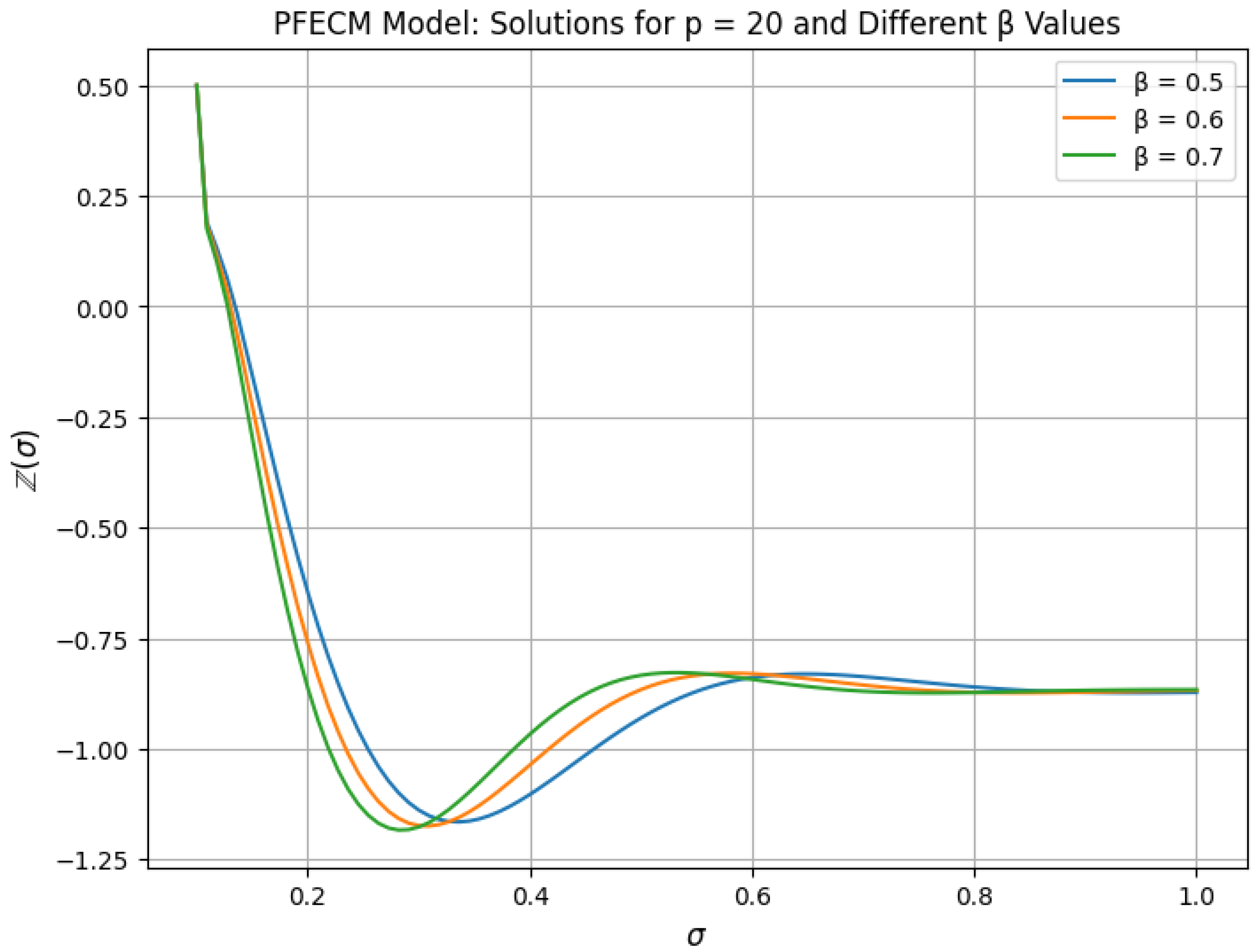
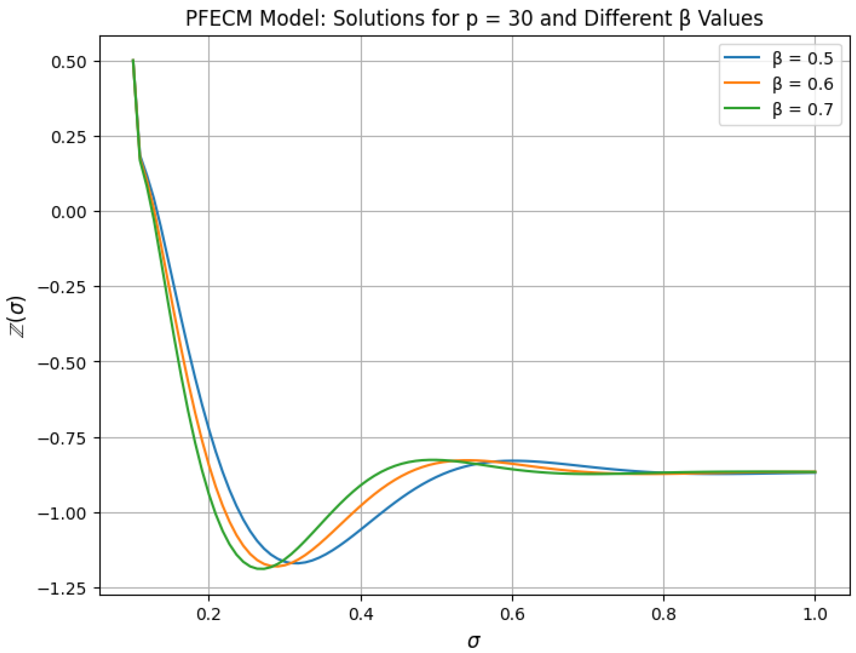
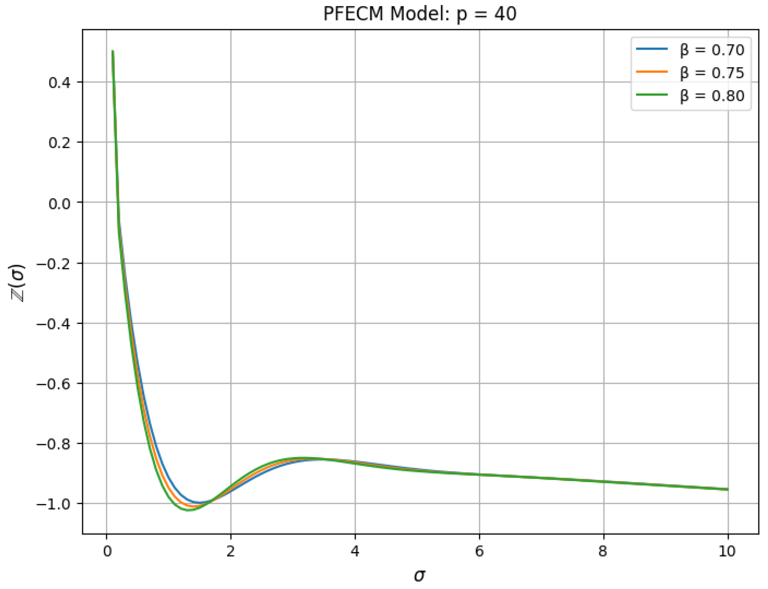
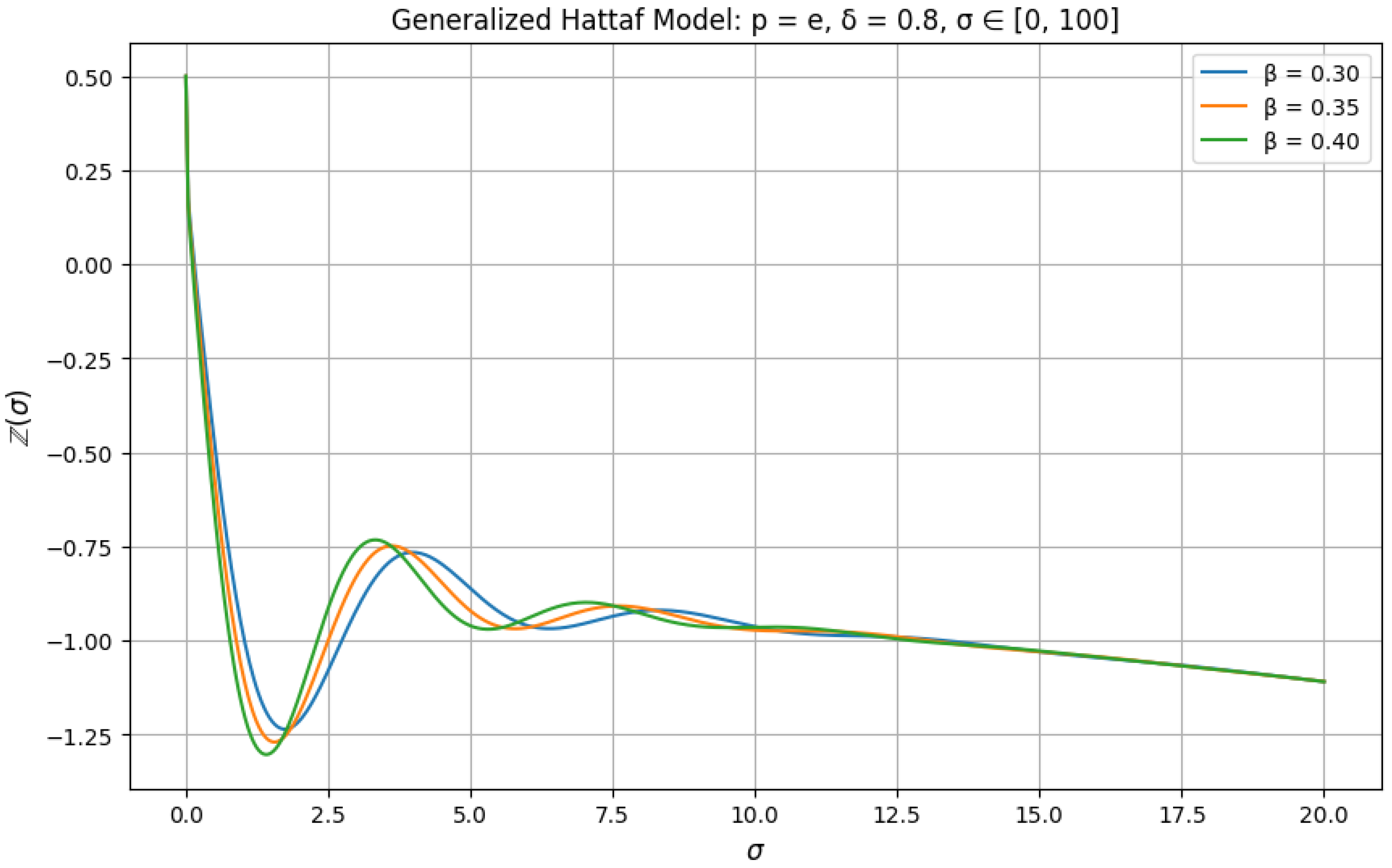
5. Examples and Simulation Results

Let us consider the following the PFECM:
D σ , w β , δ , p a         PC Z ( σ ) sin Z ( σ ) σ 2 + 100 = exp Z ( σ ) σ 50 + Z ( σ ) 100 + Z ( σ ) , σ 0 , 1 , Z ( 0 ) = 0.5 ,
where
Z σ , Z σ = sin Z ( σ ) σ 2 + 100 , Ω Z ( σ ) = exp Z ( σ ) σ 50 , K σ , Z σ = Z ( σ ) 100 + Z ( σ ) .
By assumptions (H1–H3), we have
L K = 1 100 , L Z = 1 100 , η K = η Z = 1 100 , λ K = λ Z = 0 , Ω = 1 50 .
By Theorem 5, for p > 0 , and β , δ 0 , 1 , we have
Υ = L Z + Ω + L K 1 β PC ( β ) + ln p β PC ( β ) 1 Γ δ + 1 = 1 100 + 1 50 + 1 100 1 β PC ( β ) + ln p β PC ( β ) 1 Γ δ + 1 < 1 .
Thus, all conditions in Theorem 5 are satisfied, and hence, the model (23) has a unique solution given by
Z σ = w 0 w σ 0.5 + sin Z ( σ ) σ 2 + 100 + 0 PC I σ , w β , δ , p exp Z ( σ ) σ 50 + Z ( σ ) 100 + Z ( σ ) .
By (22), the approximate solution of (23) is given as follows:
Z σ m + 1 = w 0 w σ m 0.5 + sin Z ( σ m ) σ m 2 + 100 + 1 β PC ( β ) w ( σ m ) exp Z ( σ m ) σ m 50 + Z ( σ m ) 100 + Z ( σ m ) + ln p β h δ PC ( β ) Γ ( δ + 2 ) w σ m × l = 0 m w ( σ l 1 ) exp Z ( σ l 1 ) σ l 1 50 + Z ( σ l 1 ) 100 + Z ( σ l 1 ) A m , l δ + w ( σ l ) exp Z ( σ l ) σ l 50 + Z ( σ l ) 100 + Z ( σ l ) B m , l δ ,
where
A m , l δ = m l δ m l + 1 + δ m l + 1 δ + 1 , B m , l δ = m l + 1 δ m l + 2 + δ m l δ m l + 2 + 2 δ .
The numerical approximate solution of (23) with different fractional order β , δ = 1 2 , p = 10 , p = 20 , p = 30 , p = 40 and weight function w σ = σ + 2 , is displayed in Figure 1, Figure 2, Figure 3 and Figure 4.

Symmetric Cases

  • Case 1: If p = e . Then, the PFECM (23) is reduced to the following generalized Hattaf fractional model:
    D σ , w β , δ , e 0         PC Z ( σ ) sin Z ( σ ) σ 2 + 100 = exp Z ( σ ) σ 50 + Z ( σ ) 100 + Z ( σ ) , Z ( 0 ) = 0.5
    For p = e , and for all β , δ 0 , 1 , we have
    1 100 + 1 50 + 1 100 1 β PC ( β ) + β PC ( β ) 1 Γ δ + 1 < 1 .
    According to Corollary 1, the generalized Hattaf fractional model (24) has a unique solution given by
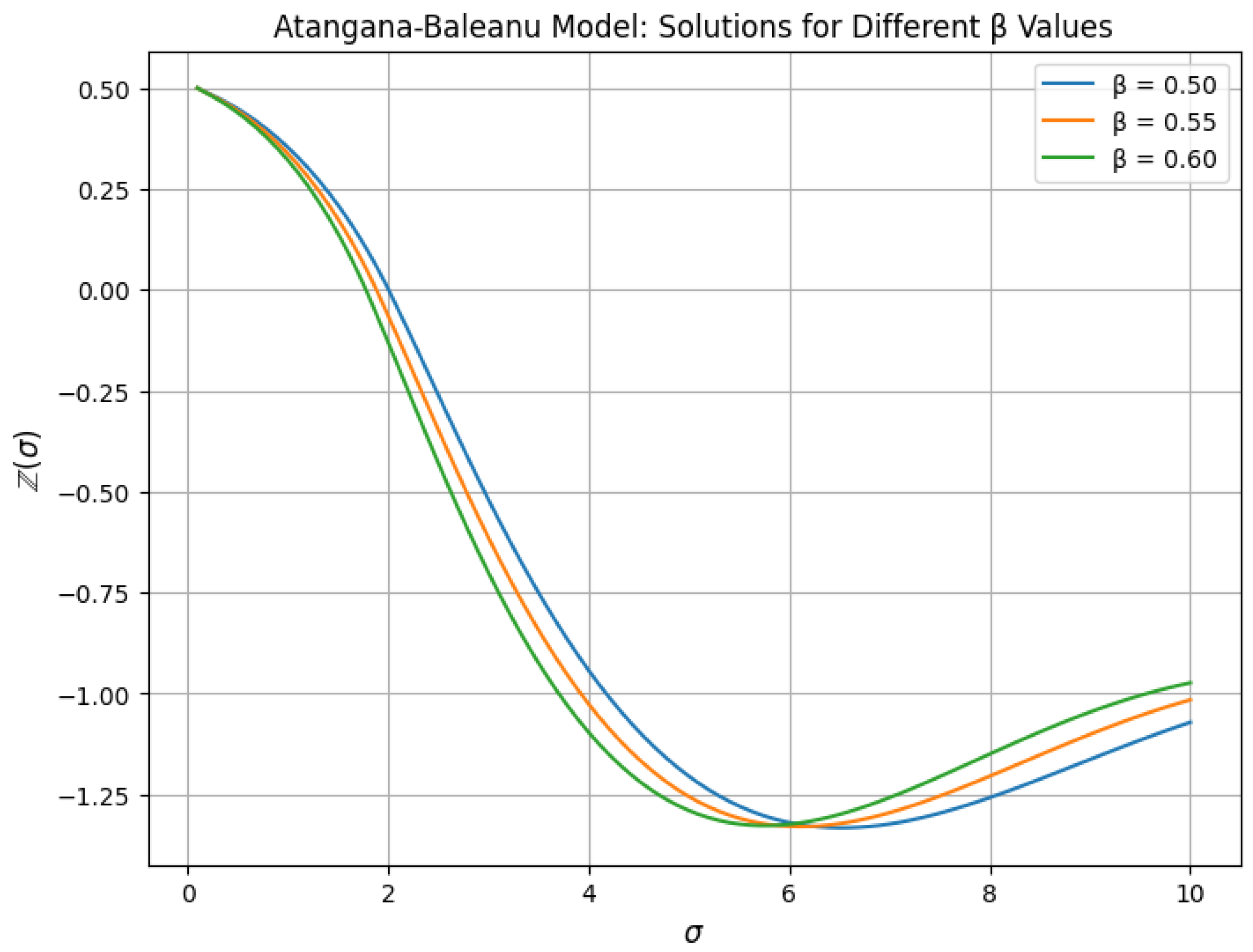
    Z σ = w 0 w σ 0.5 + sin Z ( σ ) σ 2 + 100 + 0 PC I σ , w β , δ , e exp Z ( σ ) σ 50 + Z ( σ ) 100 + Z ( σ ) .
    By (22), the approximate solution of generalized Hattaf fractional model (24) is given as follows:
    Z σ m + 1 = w 0 w σ m 0.5 + sin Z ( σ m ) σ m 2 + 100 + 1 β PC ( β ) w ( σ m ) exp Z ( σ m ) σ m 50 + Z ( σ m ) 100 + Z ( σ m ) + β h δ PC ( β ) Γ ( δ + 2 ) w σ m × l = 0 m w ( σ l 1 ) exp Z ( σ l 1 ) σ l 1 50 + Z ( σ l 1 ) 100 + Z ( σ l 1 ) A m , l δ + w ( σ l ) exp Z ( σ l ) σ l 50 + Z ( σ l ) 100 + Z ( σ l ) B m , l δ ,
    where
    A m , l δ = m l δ m l + 1 + δ m l + 1 δ + 1 , B m , l δ = m l + 1 δ m l + 2 + δ m l δ m l + 2 + 2 δ .
    The numerical approximate solution of generalized Hattaf fractional model (24) with different fractional order β 0 , 1 , δ = 1 2 , p = e , and weight function w σ = σ + 2 , is displayed in Figure 5.
  • Case 2: If δ = β , p = e , and w σ = 1 , then the model (23) is reduced to the following Atangana–Baleanu fractional model:
    D σ , 1 β , β , e a         PC Z ( σ ) sin Z ( σ ) σ 2 + 100 = exp Z ( σ ) σ 50 + Z ( σ ) 100 + Z ( σ ) , Z ( a ) = 0.5 ,
    For all δ = β 0 , 1 , p = e and w σ = 1 , we have
    1 100 + 1 50 + 1 100 1 β PC ( β ) + β PC ( β ) 1 Γ β + 1 < 1 .
    According to Corollary 2, the Atangana–Baleanu fractional model (25) has a unique solution given by
    Z σ = 0.5 + sin Z ( σ ) σ 2 + 100 + 0 PC I σ , 1 β , β , e exp Z ( σ ) σ 50 + Z ( σ ) 100 + Z ( σ ) .
    By (22), the approximate solution of the Atangana–Baleanu fractional model (25) is given as follows:
    Z σ m + 1 = 0.5 + sin Z ( σ m ) σ m 2 + 100 + 1 β PC ( β ) exp Z ( σ m ) σ m 50 + Z ( σ m ) 100 + Z ( σ m ) + β h β PC ( β ) Γ ( β + 2 ) × l = 0 m exp Z ( σ l 1 ) σ l 1 50 + Z ( σ l 1 ) 100 + Z ( σ l 1 ) A m , l β + exp Z ( σ l ) σ l 50 + Z ( σ l ) 100 + Z ( σ l ) B m , l β ,
    where
    A m , l β = m l β m l + 1 + β m l + 1 β + 1 , B m , l β = m l + 1 β m l + 2 + β m l β m l + 2 + 2 β .
    The numerical approximate solution of the Atangana–Baleanu fractional model (25) with different fractional order β 0 , 1 , p = e , and weight function w σ = 1 , is displayed in Figure 6.
  • Case 3: If δ = 1 , p = e and w σ = 1 . Then, the model (23) is reduced to the following Caputo–Fabrizio fractional model:
    D σ , 1 β , 1 , e a         PC Z ( σ ) sin Z ( σ ) σ 2 + 100 = exp Z ( σ ) σ 50 + Z ( σ ) 100 + Z ( σ ) , Z ( a ) = 0.5 ,
    For δ = 1 , β 0 , 1 , p = e , and w σ = 1 , we have
    1 100 + 1 50 + 1 100 1 β PC ( β ) + β PC ( β ) σ Γ 2 < 1 .
    According to Corollary 3, the Caputo–Fabrizio fractional model (26) has a unique solution given by
    Z σ = 0.5 + sin Z ( σ ) σ 2 + 100 + a PC I σ , 1 β , 1 , e exp Z ( σ ) σ 50 + Z ( σ ) 100 + Z ( σ ) .
    By (22), the approximate solution of the Caputo–Fabrizio fractional model (26) is given as follows:
    Z σ m + 1 = 0.5 + sin Z ( σ m ) σ m 2 + 100 + 1 β PC ( β ) exp Z ( σ m ) σ m 50 + Z ( σ m ) 100 + Z ( σ m ) + β h PC ( β ) Γ ( 3 ) × l = 0 m exp Z ( σ l 1 ) σ l 1 50 + Z ( σ l 1 ) 100 + Z ( σ l 1 ) A m , l + exp Z ( σ l ) σ l 50 + Z ( σ l ) 100 + Z ( σ l ) B m , l ,
    where
    A m , l = m l m l + 1 + δ m l + 1 2 , B m , l = m l + 1 m l + 3 m l m l + 4 .
    The numerical approximate solution of the Caputo–Fabrizio fractional model (26) with different fractional order β 0 , 1 , p = e , δ = 1 , and weight function w σ = 1 , is displayed in Figure 7.

6. Discussion

Figure 1, Figure 2, Figure 3 and Figure 4 present numerical solutions of the Power Fractional Evolution Control Model (PFECM), examining the influence of both the fractional order β and the power parameter *p*. Figure 1 (p = 10) demonstrates that solutions exhibit an initial sharp negative deflection, followed by damped oscillations, and ultimately converge to zero. Increasing β leads to a less pronounced initial dip, smaller oscillation amplitudes, and a slightly accelerated decay. In Figure 2 (p = 20), similar patterns persist, yet the amplitude and decay rates are modulated, indicating the influence of the power parameter. As evident in Figure 3 (p = 30), as the power parameter increases, the differences among solutions with varying β values diminish, with the initial deflection exhibiting a more uniform response across β . In Figure 4 (p = 40), the model shows reduced oscillations, faster and smoother decay to zero, and a convergence of the solutions with different fractional orders. Notably, when β approaches 0 ( β < 0.3 ), the solutions show an increasingly slow convergence and behavior resembling that of an integral operator. As β increases towards 1 ( β > 0.8 ), the solutions exhibit a faster and smoother convergence to zero. This indicates a tendency toward behaviors resembling the traditional integer-order derivatives. These results highlight the model’s capacity to generate diverse dynamical behaviors with adjustments in both β and *p*, and the clear sensitivity of the model to the input parameters. Increased power parameter values lead to less sensitivity with respect to variations in β , and a smoother transition to zero, indicating a modulation of the memory effects by these parameters.
Figure 5 depicts solutions of the generalized Hattaf fractional model ( p = e , δ = 0.8 ), varying the fractional order β (0.30, 0.35, and 0.40). The solutions exhibit damped oscillations converging towards zero, initiated by a pronounced initial drop. These oscillations decay comparatively faster than in previous figures, and an inverse relationship between β and oscillation frequency and amplitude is observed. This highlights the Hattaf model’s capacity, as a special case of the PFECM, to display varying dynamics solely by modulating β , making it apt for capturing rapid decay phenomena. We also observed that as β approaches 0.30, the solutions decay more slowly, while the solution is smoother as β approaches 0.40.
Figure 6 presents solutions for the Atangana–Baleanu fractional model, varying the fractional order β (0.50, 0.55, and 0.6). The solutions exhibit a negative initial drop, oscillatory behavior, and convergence to zero. The initial dip has a greater magnitude at lower β values, with the convergence becoming smoother as β increases. The model demonstrates a stable transition and its capacity to represent diverse dynamical systems, with a behavior that depends on the fractional order β . We observe that at the small fractional order values ( β = 0.50 ) there is a higher amplitude and a longer decay, while as the order increases to β = 0.60 , there is a smoother and faster convergence to zero. This again shows that the behavior of the model is sensitive to variations in fractional order.
Figure 7 presents solutions for the Caputo–Fabrizio fractional model, varying the fractional order β . The solutions display a less pronounced initial negative deflection and slower oscillations compared to previous models. The oscillatory behavior is consistent with smooth convergence towards zero, which is more stable compared to the Atangana–Baleanu model. This demonstrates the Caputo–Fabrizio model’s capacity to capture memory effects and its suitability for representing dynamical systems with smoother transitions than the Hattaf and Atangana–Baleanu models. As β increases from 0.50 to 0.60, the model transitions from an oscillatory to a smoother behavior.
Comparative Summary:
The Power Fractional Evolution Control Model (PFECM) solutions (Figure 1, Figure 2, Figure 3 and Figure 4) demonstrate a high degree of adaptability, exhibiting distinct dynamical behaviors through the modulation of both power parameter (*p*) and fractional order β . The generalized Hattaf model (Figure 5) is shown to capture fast decaying dynamics with rapid oscillations, highlighting its suitability for representing systems with quick transients. The Atangana–Baleanu model (Figure 6) displays a characteristic oscillatory response, with convergence behavior influenced by β , making it suitable for modeling memory-dependent processes. The Caputo–Fabrizio model (Figure 7) is characterized by slower oscillations and smoother convergence, suggesting its applicability in modeling dynamical processes with gradual transitions.
Overall Significance:
The numerical results validate the feasibility of numerically solving the proposed model and its capacity to represent the complex behavior of fractional-order models. The model offers substantial flexibility in capturing different dynamics through parameter modulation, and it is capable of specializing to the Hattaf, Atangana–Baleanu, and Caputo–Fabrizio models. Furthermore, the figures underscore the sensitivity of the models response to parameter variations, highlighting the significance of selecting proper parameter values in a modeling procedure.

7. Conclusions

This study investigated the existence, uniqueness, and Hyers–Ulam stability of solutions for nonlinear fractional evolution control systems using a novel approach based on power non-local kernels. This framework, employing a generalized fractional derivative (the PFD) that encompasses Caputo–Fabrizio, Atangana–Baleanu, and generalized Hattaf derivatives as special cases, provides a flexible and powerful tool for modeling complex systems with memory effects. The tunable power parameter inherent in the PFD enables fine-grained control over the memory effects captured by the model. Our key findings are summarized as follows:
  • Establishment of Existence and Uniqueness: Using fixed-point theory, we rigorously proved the existence and uniqueness of solutions for the nonlinear fractional evolution control system under appropriate conditions. This result holds for the generalized fractional derivative with a power non-local kernel, and thus encompasses the specific cases of the aforementioned established derivatives.
  • Demonstration of Hyers–Ulam Stability: We established the Hyers–Ulam stability of the system, demonstrating the robustness of the solutions against small perturbations. This property, combined with our numerical scheme based on Lagrange interpolation polynomials, is crucial for ensuring the reliability of numerical approximations and the practical applicability of the model to real-world scenarios.
  • Versatile Tool for Complex System Modeling: This flexible framework introduces a novel power fractional derivative, provides strong theoretical results, and presents a practical numerical method. The PFD approach represents a significant advancement in modeling systems with intricate memory processes, opening new avenues for research in fractional calculus and its diverse applications.
  • Numerical Validation of Model Adaptability: Our numerical results demonstrate the proposed model’s adaptability to a wide range of dynamics. The findings highlight the significance of the power non-local kernel for fractional-order modeling, along with its ability to fine-tune model behavior through both the power parameter and fractional order, making it suitable for representing complex dynamical behaviors.
Future research will focus on developing efficient numerical methods specifically tailored to power non-local kernel derivatives, alongside investigations into their practical applications in real-world problems. This will include exploring the impact of the power fractional derivative (PFD) on nonlinear wave equations, particularly the nonlinear Schrödinger (NLS) and modified Korteweg–de Vries (mKdV) models, where exploring solutions to their Cauchy problems may unveil new dynamics and solution phenomena arising from the PFD’s memory and tunable properties, such as the emergence of novel solitons, breathers, and rogue waves.

Author Contributions

Conceptualization, M.A.; Methodology, F.G., M.A., O.O., B.M. and N.E.; Formal analysis, M.A., O.O. and A.K.; Investigation, K.A.; Writing—original draft, F.G., M.A., O.O., B.M., K.A., A.K. and N.E. writing—review and editing, M.A. and K.A. All authors have read and agreed to the published version of the manuscript.

Funding

This research received no external funding.

Data Availability Statement

Data are contained within the article.

Acknowledgments

The researchers would like to thank the Deanship of Graduate Studies and Scientific Research at Qassim University for financial support (QU-APC-2025).

Conflicts of Interest

The authors declare no conflicts of interest.

References

  1. Podlubny, I. Fractional Differential Equations; Academic Press: San Diego, CA, USA, 1999. [Google Scholar]
  2. Samko, S.G.; Kilbas, A.A.; Marichev, O.I. Fractional Integrals and Derivatives; Gordon & Breach: Yverdon, Switzerland, 1993. [Google Scholar]
  3. Magin, R.L. Fractional Calculus in Bioengineering; Begell House: Redding, CA, USA, 2006. [Google Scholar]
  4. Kilbas, A.A.; Srivastava, H.M.; Trujillo, J.J. Theory and Applications of Fractional Differential Equations; North-Holland Mathematics Studies; Elsevier: Amsterdam, The Netherlands, 2006. [Google Scholar]
  5. Baleanu, D.; Diethelm, K.; Scalas, E.; Trujillo, J.J. Fractional Calculus. In Series on Complexity, Nonlinearity and Chaos; World Scientific Publishing Co., Pte. Ltd.: Hackensack, NJ, USA, 2012; Volume 3. [Google Scholar]
  6. Srivastava, H.M.; Saad, K.M. Some new models of the time-fractional gas dynamics equation. Adv. Math. Models Appl. 2018, 3, 5–17. [Google Scholar]
  7. Algahtani, O.J.J. Comparing the Atangana–Baleanu and Caputo–Fabrizio derivative with fractional order: Allen Cahn model. Chaos Solitons Fractals 2016, 89, 552–559. [Google Scholar] [CrossRef]
  8. Oliveira, E.C.D.; Machado, J.A. A review of definitions for fractional derivatives and integral. Math. Probl. Eng. 2014, 1–7. [Google Scholar] [CrossRef]
  9. Bayın, S.Ş. Definition of the Riesz derivative and its application to space fractional quantum mechanics. J. Math. Phys. 2016, 57, 123501. [Google Scholar] [CrossRef]
  10. Ma, L.; Li, C. On Hadamard fractional calculus. Fractals 2017, 25, 1750033. [Google Scholar] [CrossRef]
  11. Ferrari, F. Weyl and Marchaud derivatives: A forgotten history. Mathematics 2018, 6, 6. [Google Scholar] [CrossRef]
  12. Anderson, D.R.; Ulness, D.J. Properties of the Katugampola fractional derivative with potential application in quantum mechanics. J. Math. Phys. 2015, 56, 063502. [Google Scholar] [CrossRef]
  13. Caputo, M.; Fabrizio, M. Applications of new time and spatial fractional derivatives with exponential kernels. Prog. Fractional Differ. Appl. 2016, 2, 1–11. [Google Scholar] [CrossRef]
  14. Shah, K.; Sher, M.; Abdeljawad, T. Study of evolution problem under Mittag–Leffler type fractional order derivative. Alex. Eng. J. 2020, 59, 3945–3951. [Google Scholar] [CrossRef]
  15. Alraqad, T.; Almalahi, M.A.; Mohammed, N.; Alahmade, A.; Aldwoah, K.A.; Saber, H. Modeling Ebola Dynamics with a Φ-Piecewise Hybrid Fractional Derivative Approach. Fractal Fract. 2024, 8, 596. [Google Scholar] [CrossRef]
  16. Aldwoah, K.A.; Almalahi, M.A.; Hleili, M.; Alqarni, F.A.; Aly, E.S.; Shah, K. Analytical study of a modified-ABC fractional order breast cancer model. J. Appl. Math. Comput. 2024, 70, 1–32. [Google Scholar]
  17. Aldwoah, K.A.; Almalahi, M.A.; Abdulwasaa, M.A.; Shah, K.; Kawale, S.V.; Awadalla, M.; Alahmadi, J. Mathematical analysis and numerical simulations of the piecewise dynamics model of Malaria transmission: A case study in Yemen. AIMS Math 2024, 9, 4376–4408. [Google Scholar] [CrossRef]
  18. Kavitha, K.; Vijayakumar, V.; Udhayakumar, R.; Nisar, K.S. Results on the existence of Hilfer fractional neutral evolution equations with infinite delay via measures of noncompactness. Math. Appl. Sci. 2021, 44, 1438–1455. [Google Scholar] [CrossRef]
  19. Raja, M.; Vijayakumar, V.; Udhayakumar, R.; Nisar, K.S. Results on existence and controllability results for fractional evolution inclusions of order 1 < r < 2 with Clarke’s subdifferential type. Numer. Methods Partial. Differ. Equ. 2024, 40, e22691. [Google Scholar]
  20. Saber, H.; Almalahi, M.A.; Albala, H.; Aldwoah, K.; Alsulami, A.; Shah, K.; Moumen, A. Investigating a Nonlinear Fractional Evolution Control Model Using W-Piecewise Hybrid Derivatives: An Application of a Breast Cancer Model. Fractal Fract. 2024, 8, 735. [Google Scholar] [CrossRef]
  21. Almalahi, M.A.; Ibrahim, A.B.; Almutairi, A.; Bazighifan, O.; Aljaaidi, T.A.; Awrejcewicz, J. A qualitative study on second-order nonlinear fractional differential evolution equations with generalized ABC operator. Symmetry 2022, 14, 207. [Google Scholar] [CrossRef]
  22. Atangana, A.; Baleanu, D. New fractional derivatives with nonlocal and non-singular kernel: Theory and application to heat transfer model. Therm. Sci. 2016, 20, 763–769. [Google Scholar] [CrossRef]
  23. Caputo, M.; Fabrizio, M. A new definition of fractional derivative without singular kernel. Prog. Fract. Differ. Appl. 2015, 1, 73–85. [Google Scholar]
  24. Hattaf, K. A new generalized definition of fractional derivative with non-singular kernel. Computation 2020, 8, 49. [Google Scholar] [CrossRef]
  25. Al-Refai, M. On weighted Atangana-Baleanu fractional operators. Adv. Difference Equ. 2020, 11, 3. [Google Scholar] [CrossRef]
  26. Yadav, P.; Jahan, S.; Shah, K.; Peter, O.J.; Abdeljawad, T. Fractional-order modelling and analysis of diabetes mellitus: Utilizing the Atangana-Baleanu Caputo (ABC) operator. Alex. Eng. J. 2023, 81, 200–209. [Google Scholar] [CrossRef]
  27. Aldwoah, K.A.; Almalahi, M.A.; Shah, K. Theoretical and numerical simulations on the hepatitis B virus model through a piecewise fractional order. Fractal Fract. 2023, 7, 844. [Google Scholar] [CrossRef]
  28. Khan, H.; Alzabut, J.; Alfwzan, W.F.; Gulzar, H. Nonlinear dynamics of a piecewise modified ABC fractional-order leukemia model with symmetric numerical simulations. Symmetry 2023, 15, 1338. [Google Scholar] [CrossRef]
  29. Lee, S.; Kim, H.; Jang, B. A Novel Numerical Method for Solving Nonlinear Fractional-Order Differential Equations and Its Applications. Fractal Fract. 2024, 8, 65. [Google Scholar] [CrossRef]
  30. Azeem, M.; Farman, M.; Akgül, A.; De la Sen, M. Fractional order operator for symmetric analysis of cancer model on stem cells with chemotherapy. Symmetry 2023, 15, 533. [Google Scholar] [CrossRef]
  31. Lotfi, E.M.; Zine, H.; Torres, D.F.M.; Yousfi, N. The power fractional calculus: First definitions and properties with applications to power fractional differential equations. Mathematics 2022, 10, 3594. [Google Scholar] [CrossRef]
  32. Zitane, H.; Torres, D.F. A class of fractional differential equations via power non-local and non-singular kernels: Existence, uniqueness and numerical approximations. Phys. Nonlinear Phenom. 2024, 457, 133951. [Google Scholar] [CrossRef]
  33. Banerjee, J.; Ghosh, U.; Sarkar, S.; Das, S. A study of fractional Schrödinger equation composed of Jumarie fractional derivative. Pramana 2017, 88, 1–15. [Google Scholar] [CrossRef]
  34. Tyagi, A.K.; Chandel, J. Solution of Inhomogeneous Linear Fractional Differential Equations Involving Jumarie Fractional Derivative. J. Sci. Res. 2023, 15, 672–693. [Google Scholar] [CrossRef]
  35. Yue, Y.; He, L.; Liu, G. Modeling and application of a new nonlinear fractional financial model. J. Appl. Math. 2013, 1, 325050. [Google Scholar] [CrossRef]
  36. Al-Refai, M.; Jarrah, A.M. Fundamental results on weighted Caputo–Fabrizio fractional derivative. Chaos Solitons Fractals 2019, 126, 7–11. [Google Scholar] [CrossRef]
  37. Hattaf, K. On some properties of the new generalized fractional derivative with non-singular kernel. Math. Probl. Eng. 2021, 6, 1580396. [Google Scholar] [CrossRef]
  38. Ibrahim, R.W. Generalized Hyers-Ulam stability for fractional differential equations. Int. J. Math. 2012, 23, 1250056. [Google Scholar] [CrossRef]
Figure 1. Graphical presentations of the PFECM (23) for p = 10 , using the fractional orders β = 0.5 , 0.6 , and 0.7 .
Fractalfract 09 00104 g001
Figure 2. Graphical presentations of the PFECM (23) for p = 20 , using the fractional orders β = 0.5 , 0.6 and 0.7 .
Fractalfract 09 00104 g002
Figure 3. Graphical presentations of the PFECM (23) for p = 30 , using the fractional orders β = 0.5 , 0.6 , and 0.7 .
Fractalfract 09 00104 g003
Figure 4. Graphical presentations of the PFECM (23) for p = 40 , using the fractional orders β = 0.7 , 0.75 , and 0.8 .
Fractalfract 09 00104 g004
Figure 5. Graphical presentations of generalized Hattaf fractional model (24) for p = e , δ = 0.8 using fractional orders β = 0.3 , 0.35 , and 0.4 .
Fractalfract 09 00104 g005
Figure 6. Graphical presentations of Atangana–Baleanu fractional model (25) for p = e , δ = β = 0.5 , 0.55 , and 0.6 , and weight function w σ = 1 .
Fractalfract 09 00104 g006
Figure 7. Graphical presentations of Caputo–Fabrizio fractional model (26) for δ = 1 , p = e , with fractional order β = 0.5 , 0.55 , 0.6 , and weight function w σ = 1 .
Fractalfract 09 00104 g007
Disclaimer/Publisher’s Note: The statements, opinions and data contained in all publications are solely those of the individual author(s) and contributor(s) and not of MDPI and/or the editor(s). MDPI and/or the editor(s) disclaim responsibility for any injury to people or property resulting from any ideas, methods, instructions or products referred to in the content.

