Nonlinear Analysis of the U.S. Stock Market: From the Perspective of Multifractal Properties and Cross-Correlations with Comparisons

Abstract

This study investigates the multifractal properties of daily returns of the Standard and Poor’s 500 Index (SPX), the Dow Jones Industrial Average (DJI), and the Nasdaq Composite Index (IXIC), the three main indices representing the U.S. stock market, from 1 January 2005 to 1 November 2024. The multifractal detrended fluctuation analysis (MF-DFA) method is applied in this study. The origins of the multifractal properties of these returns are both long-range correlation and fat-tail distribution properties. Our findings show that the SPX exhibits the highest multifractal degree, and the DJI exhibits the lowest for the whole sample. This study also examines the multifractal behaviors of cross-correlations among the three major indices through the multifractal detrended cross-correlation analysis (MF-DCCA) method. It is concluded that the indices are cross-correlated and the cross-correlations also exhibit multifractal properties. Meanwhile, these returns exhibit different multifractal properties in different stages of the market, which shows some asymmetrical dynamics of the multifractal properties. These empirical results may have some important managerial and academic implications for investors, policy makers, and other market participants.

1. Introduction

Mandelbrot (1999) [1] introduced the concept of multifractality, which was viewed as great challenges to the efficient market hypothesis (EMH). According to Peters (1994) [2], financial market behaviors can be more accurately predicted by the fractional Brownian motion. It can well explain the market irregularities, including nonlinearity, self-similarity, asymmetry, long-dependence, fat tails, etc.

As the main source of capital for U.S. companies, the U.S. stock market can regulate the flow of capital and the direction of investments, causing a direct or indirect impact on the adjustment and optimization of the U.S. economic structure. The U.S. stock market is one of the most developed stock markets in the world. It is a mature market with large-scale and standardized operations. The three most significant indices among the major stock price indices in the market are the Standard and Poor’s 500 Index (SPX), the Dow Jones Industrial Average (DJI), and the Nasdaq Composite Index (IXIC), which are representative of the changing trends in the U.S. stock market and can be considered as effective indicators of the U.S. economy to a certain extent. Different from previous studies, this study systematically examines the SPX, the DJI, and the IXIC returns from multifractal, cross-correlation, and dynamic perspectives. This study mainly investigates the multifractal properties and cross-correlations in the U.S. stock market from 2005 to 2024. First, this study applies the multifractal detrended fluctuation analysis (MF-DFA) method to quantitatively analyze the multifractal properties of the SPX, the DJI, and the IXIC returns. We empirically study the market risk and efficiency level based on the main multifractal parameters. The findings of this study confirm that the returns in the U.S. stock market exhibit multifractal properties. Second, this study attempts to empirically investigate the multifractal properties of the cross-correlations among the SPX, the DJI, and the IXIC returns by the multifractal detrended cross-correlation analysis (MF-DCCA) method, which shows that the three indices in the U.S. stock market are cross-correlated and the cross-correlations also exhibit significant multifractal properties. The properties of the cross-correlations among these returns may help study the U.S. stock market from a systematic perspective. Third, we compare the differences between the multifractal properties during different periods by dividing the sample into two different stages. This may be helpful in understanding the dynamics of the multifractal properties. Specifically, we select two stages representative of price changes in the U.S. market: one represents a long-term trend of steady growth in stock prices, and the other represents the opposite trend of stock prices. Empirical results on the multifractal properties of the U.S. stock market indicate that the U.S. stock market is a complex, nonlinear, and dynamic system. Accordingly, this requires investors and regulators to make decisions in a more systematic and comprehensive way. This study provides certain theoretical and practical values for producing evidence relating to financial risk contagions in the U.S. stock market.

The rest of the paper is organized as follows. Section 2 provides a brief literature review. Section 3 introduces the research methodology. Section 4 describes the data and presents preliminary statistics. Section 5 shows empirical results. Section 6 concludes this paper.

2. Literature Review

Recent studies on the volatility and efficiency in the U.S. stock market show that the stock market is a complex system with nonlinear structural properties and encounters extreme event shocks. Seth and Sharma (2015) [3] examined the efficiency and integration of Asian and U.S. stock markets and tested the effects of financial crisis, finding that the U.S. stock markets is inefficient in weak form. Ito et al. (2016) [4] studied the efficiency of the U.S. stock market by a time-varying autoregressive model and found that the U.S. stock market efficiency has evolved over time with a considerably long periodicity. Benkraiem et al. (2018) [5] examined the effects of the energy price fluctuations on the S&P 500 prices by the quantile autoregressive distributed lags (QARDL) model and showed an asymmetric and nonlinear impact transmitting from the energy price shocks to the U.S. stock market prices. Kyle et al. (2020) [6] studied the invariance relationships in tick-by-tick transaction data in the U.S. stock market and concluded that changes in monthly regression coefficients are outcomes of rising significance of minimum lot size where algorithmic traders split orders into tiny pieces. Oleg et al. (2022) [7] investigated the networks of causal relationships in the U.S. stock market and suggested that the considered network properties may remarkably change when some significant global-scale events happen. Moreover, Beckmann et al. (2024) [8] suggested that stock market reactions of the U.S. banks to speeches by the U.S. Federal Reserve (FED) executives indicating that they intend to introduce a CBDC (Central Bank Digital Currency) are more negative when these banks depend more on deposits.

Ammy-Driss and Garcin (2023) [9] put forward a dynamic estimation method for efficiency indicators and focused on the impacts of the COVID-19 pandemic on financial markets and the efficiency of these markets. They found that the U.S. financial markets are less efficient during the COVID-19 pandemic. Conversely, Asian and Australian markets are less affected. Belhoula et al. (2024) [10] focused on the efficiency in European natural gas markets during the COVID-19 and Russia–Ukraine crises. They found higher multifractal properties under different trends during the COVID-19 pandemic and the Russia–Ukraine conflict. The market inefficiencies during these crises can be attributed to speculative strategies. Sharif et al. (2024) [11] investigated the influence of COVID-19 on the returns of energy indices in the U.S. with daily time series data of WTI and Brent markets. They suggested that the COVID-19 pandemic had significant effects on the volatility of the U.S. energy commodity indices. Choi et al. (2024) [12] studied the impact of the COVID-19 pandemic on the Korean and U.S. labor markets. They found that the COVID-19 pandemic had the most considerable effects on the Korean not-at-work rate and the U.S. unemployment rate.

Benjamin et al. (2022) [13] focused on the impacts of high-frequency trading on securities markets and suggested that the effects on liquidity and, to a lesser extent, on price volatility are substantial when high-frequency trading is interrupted. Inés et al. (2023) [14] examined high-order moment transmission between emerging and developed and digital asset markets through a flexible semi-nonparametric approach. They found a positive transmission of volatility from emerging and developed markets to digital asset markets. Kocaarslan (2024) [15] investigated the dynamic network connectedness among the U.S. oil market, monetary policy, and exchange rate dynamics. It is found that the strongest source of risk transmission is oil market uncertainty and that the cross-market spillovers are more prominent than within-market spillovers.

The MF-DFA method is frequently applied to investigate the multifractal properties of various markets. Shaw et al. (2017) [16] found the multifractal properties of fluctuations caused by the existence of significant long-term correlation through the study of the floating potential fluctuations by the MF-DFA method. Al-Yahyaee et al. (2018) [17] compared the efficiency of the Bitcoin market with gold, stock, and foreign exchange markets based on the MF-DFA method. They found that the long-memory and multifractal properties of the Bitcoin market are stronger, and the Bitcoin market exhibits higher inefficiency than the other three markets. Stosic et al. (2019) [18] studied the daily price returns for seven Brazilian market (Bovespa) sectors by the MF-DFA method and suggested that multifractal behaviors for different market sectors are rather distinct and that individual sectors exhibit different dynamics from the entire market. It was implicated that the selected stock markets, including eight developed and two emerging countries, display multifractal and long-term persistent properties with relatively higher efficiency in the long run than in the short run via long spans of data (Tiwari et al. (2019) [19]). Wang et al. (2019) [20] studied the Chinese crude oil market officially listed in the Shanghai International Energy Exchange Center (INE) by the MF-DFA method and multifractal spectrum analysis. They found that the returns of the INE crude oil exhibit significant multifractal properties, and the risk of the INE crude oil futures market is less than that of the mature crude oil futures markets. The asymmetric multifractality and efficiency in four DeFi assets (BAT-Basic Attention Token, LINK-Chainlink, MKR-Maker, and SNX-Synthetix) were also examined by the asymmetric MF-DFA approach and Hurst exponents. The results suggested that the multifractal properties are different during downward and upward trends (Mensi et al. (2023) [21]). de Salis and dos Santos Maciel (2023) [22] measured the efficiency degrees of the price returns in the cryptocurrency market through the MF-DFA method. They suggested that cryptocurrency price returns exhibit multifractality and left-sided asymmetry and that their inefficiency levels change over time, leading substantially to the multifractal spectrum. These studies employed the MF-DFA method to explore the structural properties of various markets. They suggested that the markets exhibit multifractal properties. Although the MF-DFA method is widely applied to study the multifractal properties through the Hurst exponent and multifractal spectrum, this method is mainly used to analyze the multifractal properties of a single market.

On the other hand, the MF-DCCA method can be applied to examine the properties of the cross-correlations of multiple correlated series. This may help understand the complexity of a system. Li et al. (2018) [23] examined the dynamic cross-correlations between the RMB exchange index and the liquidity of the Shanghai and Shenzhen stock markets through the MF-DCCA method. They found that the dynamic cross-correlations challenge the EMH and that the cross-correlations are of multifractal properties. They also showed that the cross-correlations exhibit positive persistence, which is strengthened under the condition of a tightening monetary policy. To study the inefficiency of the cryptocurrency market, Zhang et al. (2018) [24] constructed a value-weighted Cryptocurrency Composite Index (CCI) and employed the MF-DCCA method to investigate the cross-correlations between the CCI and the DJI, indicating that the cross-correlations between the two indices exhibit persistence and multifractal properties. Ruan et al. (2018) [25] studied the cross-correlations between the Hang Seng China Enterprises Index (HSCE) and RMB exchange markets by a cross-correlation statistic test and the MF-DCCA method, finding that the returns of the HSCE and RMB exchange markets exhibit significant cross-correlations and that the cross-correlations are of strong multifractal properties. By the MF-DCCA method, Fang et al. (2018) [26] investigated the dynamic cross-correlations between carbon emission allowance and stock returns for European and Chinese markets, respectively. The findings indicated that the cross-correlations between carbon emission allowance and stock returns exhibit significant multifractal properties in European and Chinese markets and that the cross-correlations are caused by both the persistence of fluctuations and fat-tail distributions of the considered series. Ghosh et al. (2019) [27] studied the evolving behaviors of the thoughts over a decade in both versions of the texts using chaos, finding a nonlinear pattern of correlation with a high degree of complexity. Ahmed et al. (2024) [28] used the MF-DCCA method to study the nonlinear structure and dynamic changes in the multifractal behaviors of cross-correlations between the financial stress index (FSI) and four well-known commodity indices, namely the Commodity Research Bureau Index (CRBI), Baltic Dry Index (BDI), London Metal Index (LME), and Brent Oil prices (BROIL). The results showed that the multifractal cross-correlation between FSI and BROIL is the highest and that between FSI and LME is the lowest. These studies mainly investigate the cross-correlations among different time series in various markets and find multifractal behaviors in the cross-correlations.

Generally, most previous literature applied the MF-DFA method to study multifractal properties of various markets and the MF-DCCA method to study cross-correlations among various series. Although some previous studies studied the U.S. stock market in terms of price behaviors and efficiency, they rarely studied the dynamic multifractal properties in the U.S. stock market, especially the properties under different market trends.

3. Methodology

3.1. MF-DFA

Introduced by Kantelhardt et al. (2002) [29], the MF-DFA method is a powerful tool for investigating the multifractal properties of series. It has been applied in different fields, including energy markets [30,31], stock markets [32,33], exchange markets [34], and international capital flows [35]. Let $\left\{x_t\right\}$, t = 1, 2, …, N be a considered time series, where N is the length of the series. Steps to conduct the MF-DFA method are illustrated as follows.

Step 1. Define the profile of this series as X(i) and calculate the profile as

$$X\left(i\right)=\sum _{t=1}^i[x_t-\overline{x}]$$

(1)

where

$$\overline{x}={\displaystyle \frac{1}{N}}\sum _{t=1}^N{x}_t$$

(2)

Step 2. Divide the profile {X(i)} into N_s non-overlapping segments of equal length s, where N_s = int(N/s). If the length N of the profile is not a multiple of the considered time scale s, a short part at the end of the series will remain. To retain this part of the series, the same procedure is repeated starting from the opposite end. Thereby, we can obtain 2N_s segments altogether through twice division for each s value. According to the MF-DFA method, we set 10 < s < N/4.

Step 3. We use the OLS (optimal least square) method to fit the series and obtain the local trend for each segment. Here, $\widehat{y_v\left(i\right)}$ is the fitting polynomial with order m in segment v, and it can be calculated by

$$y_v\left(i\right)={\alpha }_0+{\alpha }_{1}i+\cdots +{\alpha }_k{i}^k$$

(3)

where i = 1, 2, …, s, k = 1, 2, ….

For each segment v, the variance for the segments can be calculated by:

$$F^2\left(s,v\right)=\left\{\begin{array}{c}{\displaystyle \frac{1}{s}}{\displaystyle \sum _{i=1}^s}{\left\{y\left[\left(v-1\right)s+i\right]-\widehat{y_v\left(i\right)}\right\}}^2,forv=1,\dots ,N_s\\ {\displaystyle \frac{1}{s}}{\displaystyle \sum _{i=1}^s}{\left\{y\left[N-\left(v-N_s\right)s+i\right]-\widehat{y_v\left(i\right)}\right\}}^2,forv=N_s+1,\dots ,{2N}_s\end{array}\right.$$

(4)

Now, we define m as the order of the fitting polynomial, and it should be appropriately set to avoid overfitting the series.

Step 4. For the whole sample, the qth order fluctuation function F_q(s) can be calculated by averaging over all the segments

$$F_q\left(s\right)={\left\{{\displaystyle \frac{1}{2N_s}}\sum _{v=1}^{2N_s}{\left[F^2\right(s,v\left)\right]}^{{\displaystyle \frac{q}{2}}}\right\}}^{{\displaystyle \frac{1}{q}}}$$

(5)

for any q ≠ 0, and

$$F_0\left(s\right)=\mathrm{e}\mathrm{x}\mathrm{p}\left\{{\displaystyle \frac{1}{4N_s}}\sum _{v=1}^{2N_s}\left[F^2\left(s,v\right)\right]\right\}$$

(6)

for q = 0.

Step 5. We repeat steps 2 to 4 for several scales s. The scaling behaviors of the fluctuation functions are determined by analyzing log–log plots of $F_q\left(s\right)$ versus s for different order q. If the series exhibits long-range power-law correlations, $F_q\left(s\right)$ will increase for large values of s as a power-law expression and the generalized Hurst exponent H(q) for s can be defined by:

$$F_q\left(s\right)\approx s^{h\left(q\right)}$$

(7)

Known as the generalized Hurst exponent, the scaling exponent H(q) represents the power-law auto-correlation of the series. The significant dependence of H(q) on q shows the multifractality of the series, whereas it is monofractal if h(q) is independent of q. For positive or negative q values, H(q) describes the scaling behaviors of the segments with large or small fluctuations, respectively. Therefore, a larger range of generalized Hurst exponent H(q) denotes a more complicated structure of the series. For q = 2, H(2) is equivalent to the Hurst exponent.

Furthermore, we can obtain the multifractal spectrum of the series by a Legendre transform. The multifractal spectrum is known as another effective way to describe a multifractal series. The range of H(q) is usually related to the multifractal level of the series. A higher △H(q_min − q_max) value always indicates stronger multifractal properties of the series.

Here, the scaling exponent $\tau \left(q\right)$ is defined by:

$$\tau \left(q\right)=qH\left(q\right)-1$$

(8)

Then, the singularity strength $h\left(q\right)$ and the singularity spectrum $D\left(q\right)$ can be obtained by the Legendre transform.

$$h\left(q\right)={\displaystyle \frac{d\tau \left(q\right)}{dq}}=H\left(q\right)+q{H}^{\prime }\left(q\right)$$

(9)

$$D\left(q\right)=qh\left(q\right)-\tau \left(q\right)=1+q\left[\alpha -H\left(q\right)\right]$$

(10)

The multifractal spectrum width is represented by the difference between h(q)_max and h(q)_min, where h(q)_max and h(q)_min denote the maximum and minimum of h(q), respectively. It also means the difference between the maximum and minimum probability from the statistical distribution perspective. As a suitable quantitative indicator of the multifractal degree of the series, the multifractal spectrum width is often employed in research on multifractal properties. In this paper, we define MD as [36]:

$$MD={h\left(q\right)}_{max}-{h\left(q\right)}_{min}$$

(11)

3.2. MF-DCCA

To study the multifractal properties of cross-correlations among financial markets, Zhou (2008) [37] proposed the MF-DCCA method. Since then, the MF-DCCA has been used to analyze the nonlinear dependency between price and volume in the agricultural commodity futures markets [38] and the portfolio strategy in global crude oil markets [39]. In this paper, we adopt the MF-DCCA method to investigate the multifractal properties of cross-correlations among main indices in the U.S. stock market. We consider two series X(i) and Y(i), where i = (1, 2, …, N). The lengths of the series X(i) and Y(i) are N. The following five steps constitute the key to the MF-DCCA method.

Step 1. Construct the profiles for the model.

$$X\left(i\right)=\sum _{t=1}^i\left[x\left(t\right)-\overline{x}\right],Y\left(i\right)=\sum _{t=1}^i\left[y\right(t)-\overline{y}],i=1,2,\dots ,N$$

(12)

where

$$\overline{x}={\displaystyle \frac{1}{N}}\sum _{t=1}^{N}x\left(t\right)and\overline{y}={\displaystyle \frac{1}{N}}\sum _{t=1}^{N}y\left(t\right)$$

(13)

Step 2. The profiles {X(i)} and {Y(i)} are subsequently separated into Ns nonoverlapping segments (or windows) of equal length s where N_s = [N/s]. As the series length N is not necessarily a multiple of the considered time-scale s, there is a relatively shorter part at the profile remaining in most cases. To consider this part of the series, we repeat the same process, which starts from the other end of the series. In this way, we can obtain 2N_s segments altogether.

Step 3. For each segment v, we can obtain the local trends X^v(i) and Y^v(i) (v = 1, 2, …, 2Ns) by fitting the considered series data for each separated segment based on the OLS method. Then, we can determine the variance by the following equation:

$$F^2\left(s,v\right)={\displaystyle \frac{1}{s}}\sum _{i=1}^s|X\left(\left(v-1\right)s+i\right)-X^v\left(i\right)|·|Y\left(\left(v-1\right)s+i\right)-Y^v\left(i\right)|$$

(14)

for each segment v, v = 1, 2, …, N_s, and

$$F^2\left(s,v\right)={\displaystyle \frac{1}{s}}\sum _{i=1}^s|X\left(N-\left(v-N_s\right)s+i\right)-X^v\left(i\right)|·|Y\left(N-\left(v-N_s\right)s+i\right)-Y^v\left(i\right)|$$

(15)

for each segment v, v = N_s + 1, …, 2N_s. Here, we use X^v(i) and Y^v(i) to represent the fitting polynomial with order k in segment v, respectively. This is conventionally called the MF-DCCA-k model. Empirically, we set the range of s to 2k + 2 ≤ s ≤ N/4.

Step 4. The q-order fluctuation function is obtained by averaging over all segments. it can be calculated as follows:

$$F_q\left(s\right)={\left\{{\displaystyle \frac{1}{2N_s}}\sum _{v=1}^{2N_s}{\left[F^2\right(s,v\left)\right]}^{{\displaystyle \frac{q}{2}}}\right\}}^{{\displaystyle \frac{1}{q}}}$$

(16)

for any q ≠ 0, and

$$F_0\left(s\right)=exp\left\{{\displaystyle \frac{1}{4N_s}}\sum _{v=1}^{2N_s}\mathrm{l}\mathrm{n}\left[F^2\right(s,v\left)\right]\right\}$$

(17)

for q = 0, where the index variable q can be any real number. For q is 2, this method is used as the standard DCCA procedure.

Step 5. We can determine the scaling behaviors of the fluctuations within the series by investigating the log–log plots of F_q(s) versus s for each q value. If the two considered series {x(i)} and {y(i)} are long-range cross-correlated, the q-order fluctuation function F_q(s) will increase for large values of s, which exhibits a power-law correlation as follow.

$$F_q\left(s\right)\approx s^{H_{xy}\left(q\right)}$$

(18)

This can be also presented as follow after taking logarithm.

$$log{F}_q\left(s\right)=H_{xy}\left(q\right)\log \left(s\right)+logA$$

(19)

The generalized cross-correlation exponent H_xy(q), which is known as the scaling exponent, describes the power-law correlation between the two time series {X(i)} and {Y(i)}. Particularly, if the series {X(i)} is identical to {Y(i)}, the MF-DCCA is equivalent to the MF-DFA. Furthermore, if the scaling exponent H_xy(q) for the two series is independent of order q, the cross-correlation between the two series exhibits monofractal properties. However, if the scaling exponent H_xy(q) for the two series is dependent on order q, the cross-correlation between the two series exhibits multifractal properties. Moreover, when q is negative, H_xy(q) indicates the scaling behaviors of the segments with relatively small fluctuations. Conversely, when q is positive, H_xy(q) indicates the scaling behaviors of the segments with relatively large fluctuations.

In this case, the bivariate Hurst exponent H_xy(2) has similar characteristics and indications as a univariate Hurst exponent. Specifically, if the Hurst exponent H_xy(2) is greater than 0.5, the cross-correlation between the two series {X(i)} and {Y(i)} is long-range persistent. If the Hurst exponent H_xy(2) is less than 0.5, the cross-correlation between the two series is anti-persistent. If the Hurst exponent H_xy(2) is equal to 0.5, the two series exhibit no cross-correlation or, at most, short-range cross-correlation.

Moreover, Yuan et al. (2012) [40] put forward ΔH as an indicator of financial risk. Similarly, we can also use ΔH to measure the degree of multifractal properties of considered series. ΔH can be determined as:

$$∆H=H_{max}\left(q\right)-H_{min}\left(q\right)$$

(20)

According to this method, a greater value of ΔH indicates a stronger degree of the multifractal properties of the series. Consequently, ΔH_xy, which can measure the degree of the multifractal properties of cross-correlations between two series, can be quantitatively obtained when H_xy(q) is substituted for H(q) in Formula (20). ΔH_xy can be calculated in a similar way.

4. Data

In this study, we choose the three most widely used indices, i.e., the SPX, the DJI, and the IXIC, to represent the U.S. stock market. The SPX represents approximately 80% of the total value of the U.S. stock market and gives a good indication of movement in the U.S. market as a whole. Known for its listing of the U.S. market’s best blue-chip companies with regularly consistent dividends, the DJI represents about a quarter of the value of the entire U.S. stock market. Changes in the IXIC generally indicate the performance of the technology sector as well as investors’ attitudes toward more speculative stocks. The daily data for the SPX, DJI, and IXIC indices are collected from the Wind database. The sample includes 7245 observations from 1 January 2005 to 1 November 2024.

Moreover, we consider two different stages to study the different multifractal properties under different trends in the U.S. stock market. The two sub-periods are:

(1)

sub-period 1: from 9 October 2007 to 6 March 2009, containing 355 observations;

(2)

sub-period 2: from 9 March 2009 to 31 March 2024, containing 5502 observations.

It is clear that the prices experienced a downward trend in sub-period 1 and a steady upward trend over a relatively long period of time in sub-period 2.

If the closing price on day t is represented by p_t, the daily returns of the SPX, the DJI, and the IXIC indices are calculated as natural logarithmic returns as:

$$r_t=\mathrm{l}\mathrm{n}\left({\displaystyle \frac{p_t}{p_{t-1}}}\right)$$

Figure 1 shows the closing prices and the logarithmic returns of the indices in the whole sample. The trends of these returns are relatively close, indicating basic correlations and consistency among the three major indices in the U.S. stock. The returns fluctuated most remarkably before and after the global financial crisis, which broke out in 2008, whereas they exhibited relatively fewer fluctuations at other times. This shows the effects of the 2008 global financial crisis on the U.S. stock market. Moreover, Figure 1 apparently shows two different market phases, the two sub-periods we consider.

For the causes of the multifractal properties, fluctuations in these returns exhibit nonlinear properties, causing long-range correlations in the series. This may be viewed as one possible reason for multifractal properties. On the other hand, the multifractal properties can also be caused by certain extreme events like the 2008 global financial crisis, which may lead to a fat-tailed distribution of the series. This may be another reason for multifractal properties.

As Figure 1 shows, the prices displayed a downward trend in sub-period 1 and exhibited a sharp fall around September 2008. The SPX and the DJI showed similar falling trends in this stage. On the contrary, the prices showed an increasing trend in sub-period 2 and exhibited a sharp growth since 2016. Overall, the fluctuations of the returns in sub-period 1 are more frequent and intense than in sub-period 2, especially during the period from October 2008 to February 2009, when the fluctuations of the returns reached the maximum degree in this period. Typically, the returns showed similarly large fluctuations around and in 2020, probably due to the COVID-19 pandemic.

The descriptive statistics of the sample are summarized in

Table 1. Descriptive statistics of daily returns of the U.S. stock market indices.

	Index	Sample Period	Number of Observations	Mean (%)	Standard Deviation	Skewness	Kurtosis
	SPX	1 January 2005~1 November 2024	7245	0.0214	0.0101	−0.6085	23.2028
Whole sample	DJI	1 January 2005~1 November 2024	7245	0.0187	0.0095	−0.5518	27.8727
	IXIC	1 January 2005~1 November 2024	7245	0.0293	0.0113	−0.4859	15.5791
	SPX	9 October 2007~6 March 2009	355	−0.2312	0.0240	−0.0595	6.7637
Sub-period 1	DJI	9 October 2007~6 March 2009	355	−0.2116	0.0219	0.1947	6.9598
	IXIC	9 October 2007~6 March 2009	355	−0.2162	0.0243	−0.0159	5.8424
	SPX	9 March 2009~31 March 2024	5502	0.0371	0.0094	−0.6176	21.7133
Sub-period 2	DJI	9 March 2009~31 March 2024	5502	0.0326	0.0090	−0.7795	30.3792
	IXIC	9 March 2009~31 March 2024	5502	0.0461	0.0108	−0.5192	14.7032

Note: “SPX”, “DJI” and “IXIC” denote the daily returns of the Standard and Poor’s 500, the Dow Jones Industrial Average, and the Nasdaq Composite indices, respectively. Data source: Wind database.

. Average returns of the three indices slightly exceed zero. The DJI has the lowest average return, and the IXIC has the highest average return. Correspondingly, the IXIC has the highest standard deviation, which confirms that the Nasdaq market has comparatively higher returns and risks. The skewness values of these returns are less than zero, which means that the distributions of returns are left-tailed. In other words, the tail on the left side of the curve seems to be longer than that on the right. Furthermore, the kurtosis values of these returns are much greater than three. This reveals that the distributions show non-Gaussian fat-tailed characteristics and are peaked with excessive kurtosis and extreme values. Hence, these returns deviate from the normal distribution, which directly contributes to the multifractal properties of the series.

In sub-period 1, the three returns are all less than zero and show a downward trend of the returns. The SPX exhibits a lower mean value in the bear market compared with the DJI and the IXIC. The skewness values of the SPX and the IXIC are less than zero, suggesting that the distributions of the two indices exhibit the distribution feature of a longer left tail in this period. Instead, the opposite occurs for the DJI. The kurtosis values of these returns are all greater than three, showing their fat-tailed distribution properties. These distribution properties are consistent with the properties obtained through the whole sample. This confirms that these returns all exhibited multifractal properties in sub-period 1.

However, in sub-period 2, the IXIC exhibits a higher mean value and standard deviation compared with the SPX and the DJI. The skewness values of these returns are less than zero, showing the distribution feature of a longer left tail in this period. The kurtosis values of these returns are all greater than three, demonstrating their fat-tailed distribution properties. These distribution properties are consistent with the properties obtained through the whole sample. This confirms that these returns all exhibit multifractal properties in sub-period 2.

5. Empirical Results

5.1. Multifractal Properties of the U.S. Stock Market

According to the MF-DFA method, generalized Hurst exponents and the multifractal spectra of the daily returns of the SPX, the DJI, and the IXIC are shown in Figure 2. As Figure 2 shows, the horizontal axis and the vertical axis represent the multifractal order value q and the Hurst exponent value, respectively. According to the MF-DFA method, the generalized Hurst exponent H(q) is an important indicator for the multifractal properties of series. The q-order generalized Hurst exponents H(q) of the SPX, the DJI, and the IXIC returns are obviously correlated to the order value q and drop smoothly with the rise in order value q. Therefore, their H(q) values are not a constant but a function of q. This means that the three returns exhibit significant multifractal properties. The H(q) values show a downward trend on the interval [−5, 5]. When q = 2, the classical Hurst exponents H(q) of the original sequence are 0.1005, 0.1056, and 0.1013, indicating negative long-range correlations in the series. The results reveal that the returns exhibit strong persistence and that the changes in these returns are opposite to the changes in the past. The spectra of the series all exhibit a single peak function, which shows the multifractal properties of the daily returns.

There are two major sources of multifractality: long-range correlations and fat-tailed distributions of volatilities. Empirically, we can study the effects of long-range correlations by the shuffling test and study the effects of the fat-tailed distributions by the phase-randomizing test. In this study, the shuffled series and the phase-randomized series are named shuf and sur, respectively. As Figure 2 shows, the Hurst exponents of the shuffled series and the phase-randomized series exhibit different structural characteristics. For the three returns, the widths of the multifractal spectra of the test series (the shuffled series and the phase-randomized series) are slightly less than that of the original series. This indicates the multifractal properties in the three original series. Moreover, the generalized Hurst exponents H(q) of the original series and test series drop when order q rises. This means that the original series of the three indices and their shuffled and phase-randomized series exhibit multifractal properties.

5.2. Multifractal Degree of the U.S. Stock Market

From the empirical results, we find that the correlations between the multifractal spectrum f(α) and the q-order singularity exponent α exhibit the shape of a single-peak bell. Figure 2 also shows the relationships between the singularity strength h(q) and the singularity spectrum D(q). The main structural parameters of the multifractal spectrum of the returns are listed in

Table 2. Multifractal properties of the returns of the U.S. stock market indices.

Index	Δα	Δf	R
SPX	1.8104	2.4475	−0.4300
DJI	1.4446	1.6499	−0.3300
IXIC	1.5452	1.5410	−0.2909

Notes: “SPX”, “DJI”, and “IXIC” denote the returns of the Standard and Poor’s 500 Index, the Dow Jones Industrial Average, and the Nasdaq Composite Index, respectively. Δα, Δf, and R denote multifractal spectrum width, distribution proportion of high values and low values and asymmetric exponent, respectively.

.

As Table 2 shows, the SPX has the highest Δα value among the three returns, and the DJI has the lowest Δα value, suggesting that the local fluctuations in the SPX are most uneven and those in the DJI are relatively most even. Therefore, the SPX exhibits the highest multifractal degree, whereas the DJI exhibits the lowest one. For the three returns, the chance of maximization of daily returns is greater than that of being at a minimum because Δf > 0. Hence, large fluctuations exist in the three original series of the returns in the U.S. stock market. The SPX has the highest Δf value among the three returns, and the IXIC has the lowest, which implies that the SPX displays the largest fluctuations and the IXIC displays the smallest fluctuations. For the three indices, the asymmetric exponents are all negative. This shows that the shapes of the multifractal spectra of these returns are left-skewed. The right half of the return Δα_R has a larger range of values. The events with lower returns have an advantage over those with higher returns. These empirical results are in line with the conclusions in Seth et al. (2015) [3] and also confirm that the U.S. stock market is not completely efficient.

5.3. Efficiency of the U.S. Stock Market

The U.S. stock market is not always efficient, and the inefficiency is partly caused by the multifractal properties of the market. The multifractal degree (MD) value is measured by the difference between α_max and α_min. A large value of MD corresponds to a high multifractal degree and low market efficiency, indicating large volatilities.

In this section, we study the asymmetrical dynamics of the multifractal properties of the U.S. stock market in terms of the multifractal degree and efficiency. The empirical results from the U.S. stock market show the asymmetries in the sub-period 1 and sub-period 2 we consider.

Table 3. Multifractal degree (MD) values of the returns in the U.S. stock market.

	Whole Sample	Sub-Period 1	Sub-Period 2	△MD
SPX	1.8104	1.1691	2.3010	1.1319
DJI	1.4446	1.4413	1.9491	0.5078
IXIC	1.5452	1.0412	1.6371	0.5959

Notes: “SPX”, “DJI”, and “IXIC” denote the returns of the Standard and Poor’s 500 Index, the Dow Jones Industrial Average, and the Nasdaq Composite Index, respectively.

shows the MD values of the three returns for the whole sample and two sub-samples.

As Table 3 shows, the SPX has the highest MD value, and the DJI has the lowest MD value for the whole sample. The multifractal properties may provide some evidence for less efficiency in the U.S. stock market.

In sub-period 2, the SPX also has the highest MD value, and the IXIC has the lowest MD value. This means that the SPX has the highest multifractal degree among the three indices under the upward trend of prices. In sub-period 1, these returns generally show lower MD than in sub-period 2. The IXIC shows the lowest MD in both sub-period 1 and sub-period 2, suggesting the lower multifractal degree in these two periods considered. Table 3 also reveals that the SPX return experiences the greatest fluctuations when the market witnessed a shift from a downward trend to an upward trend. In contrast, the DJI shows the smallest fluctuations among the three indices when the same transformation occurred because of the minimum MD change value △MD.

Therefore, the multifractal properties are different during downward and upward trends in the U.S. stock market. This asymmetry may provide some insights for market participants in terms of different properties under different trends in the market.

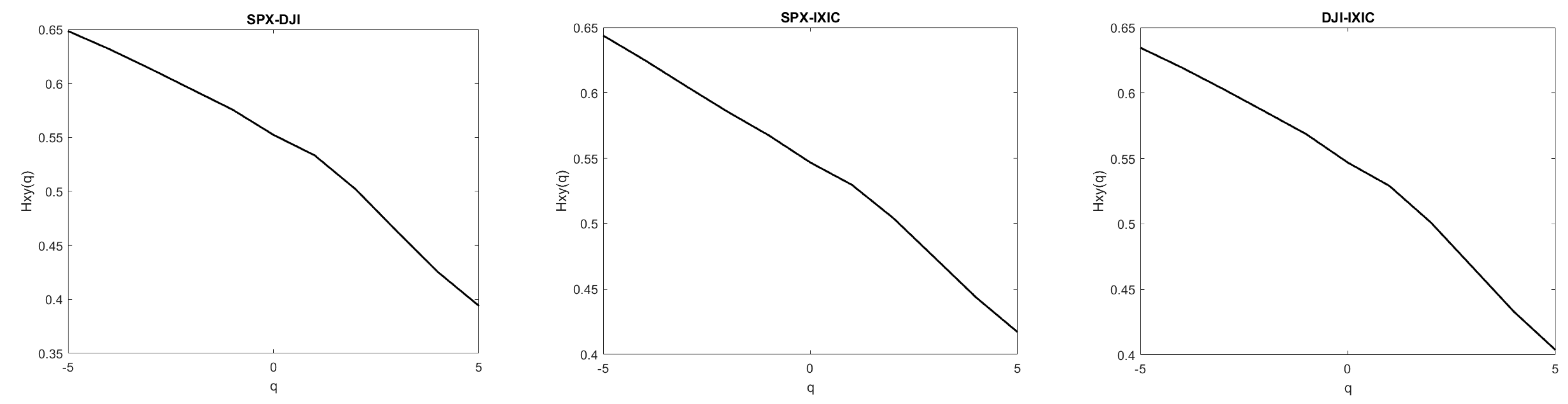
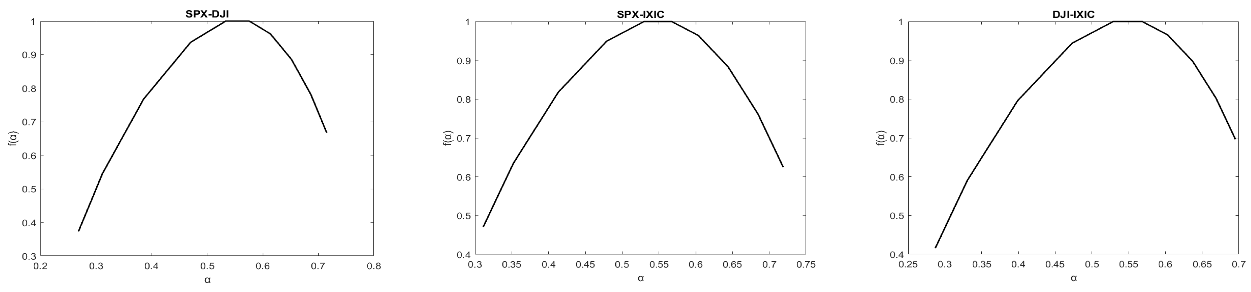
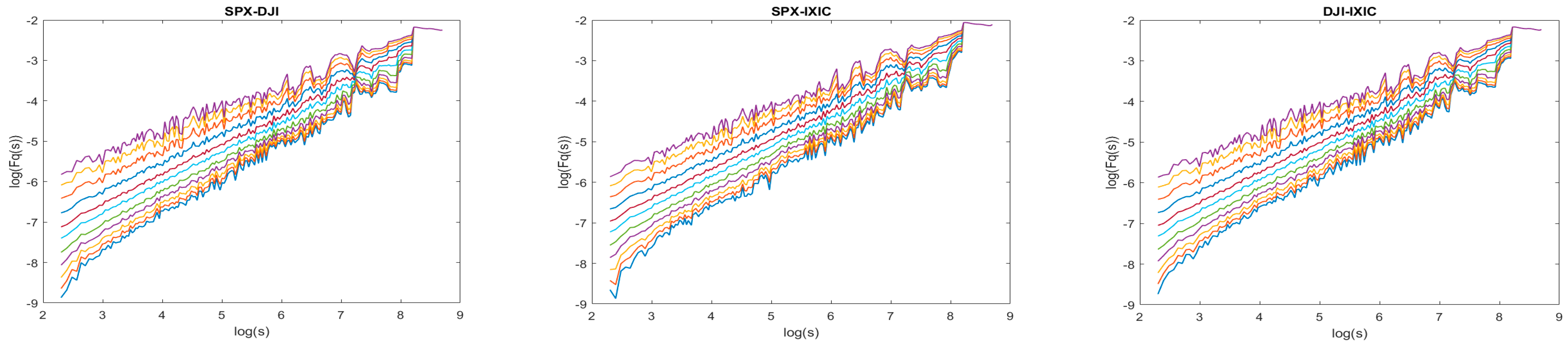
5.4. Cross-Correlations in the U.S. Stock Market

To quantitatively analyze the cross-correlations between two different returns among the SPX, the DJI, and the IXIC, we estimate the cross-correlation exponents by the MF-DCCA method. Figure 3, Figure 4, Figure 5 and Figure 6 show the cross-correlation of each pair.

In Figure 3, the relationships between generalized cross-correlation exponents H_xy(q) and the order of fluctuation function q for the SPX, the DJI, and the IXIC returns are displayed, with q varying from −5 to 5. Figure 3 shows the slopes of generalized Hurst exponents H_xy(q) across different scales ranging from −5 to 5 and reveals that H_xy(q) coefficient values are not constant and are dependent on q. This implies strong evidence for multifractal properties in the cross-correlations among the returns. As Figure 3 shows, for all three pairs of indices, H_xy(q) for small fluctuations is higher than that for large fluctuations. The scaling exponents H_xy(q) for q < 0 are larger than those for q > 0, which means that the cross-correlated behaviors of small fluctuations are more persistent than those of large fluctuations. For the three pairs of the returns, H_xy(q) functions monotonically fall for −5 ≤ q ≤ 5. The fluctuations of the three pairs of the cross-correlations may cause them to be more persistent and strengthen the cross-correlations for the interval q ≥ 2. Therefore, when there is a large fluctuation in one return in the short term, it is probably caused by the volatilities in the other two series. For the smallest fluctuations (q = −5), the cross-correlations among the returns show the strongest long-memory properties, which suggests that the long-range dependence largely explains the multifractal properties of the cross-correlations in the U.S. stock market.

Figure 4 shows the relationships between the Renyi exponents τ(q) and the order q for the three pairs of the returns. The exponent τ(q) is a strictly monotonic increasing convex function of q for −5 ≤ q ≤5. In addition, there is an obviously nonlinear relationship between τ(q) and q, confirming that the cross-correlations between the SPX and the DJI, the SPX and the IXIC, and the DJI and the IXIC returns have some multifractal properties.

Since the cross-correlations display multifractal properties, we can derive the multifractal spectra f (α) of the cross-correlations. Figure 5 shows the relationships between the multifractal spectra f (α) and the singularity exponent α for the three pairs of the returns. As Figure 5 shows, the tops of the multifractal spectrum curves f (α) are flat, and the opening of the curves is wide. The multifractal spectra f (α) are distributed in a wide range and vary with the change in the singularity exponents α. For the cross-correlation between the SPX and the DJI, f (α) reaches the minimum value of 0.3729 when α equals 0.2685 and the maximum value of 1 when α equals 0.5758. The width of multifractal spectrum of SPX-DJI pair is 0.4465. For the cross-correlation between the SPX and the IXIC, f (α) reaches the minimum of 0.4704 when α equals 0.3111 and the maximum of 1 when α equals 0.5674. The width of the multifractal spectrum of the SPX-IXIC pair is 0.4078. For the cross-correlation between the DJI and the IXIC, f (α) reaches the minimum of 0.4158 when α equals 0.2869 and the maximum of 1 when α equals 0.5685. The width of the multifractal spectrum of the DJI-IXIC pair is 0.4084. Therefore, the cross-correlations between any two returns among the SPX, the DJI, and the IXIC exhibit multifractal properties. These results are partly consistent with those of Cao et al. (2017) [41]. Particularly, the cross-correlation between the SPX and the DJI has the greatest multifractal level among the three pairs of the returns, indicating the largest volatilities. And the other two pairs have almost similar multifractal cross-correlations in terms of the multifractal spectra.

Figure 6 shows the log–log plots of log(F_q(s)) versus log(s) for each pair of the SPX, the DJI, and the IXIC returns as q =−5, −4, −3, …, 5 when polynomial order k = 2 (i.e., MF-DCCA-2, when k = 1, 3, 4, and 5, the results are qualitatively similar). Although larger fluctuations of log(F_q(s)), especially for q ≥ 2 and q ≤ −1, are observed for large values of log(s), the estimated coefficients H_xy(q) and constant log(A) in Equation (19) are all significant at the 1% significance level through the method of linear least squares. For different q values, each fluctuation curve is approximately linear. The q-order fluctuation function F_q(s) and time scales show a significant power law correlation, showing that power-law cross-correlations exist between the SPX and the DJI, the SPX, and the IXIC, the DJI and the IXIC. Therefore, the changes in fluctuations of the SPX, the DJI, and the IXIC returns are not merely affected by their own fluctuations. Specifically, the fluctuations of the DJI and the IXIC returns that are cross-correlated with the SPX return can also have effects on the fluctuations of the SPX return. The fluctuations of the SPX and the IXIC returns that are cross-correlated with the DJI return can also have effects on the fluctuations of the DJI return. The fluctuations of the SPX and the DJI returns that are cross-correlated with the IXIC return can also have effects on the fluctuations of the IXIC return. As Figure 6 shows, cross-correlations of the three pairs of returns exhibit similar properties.

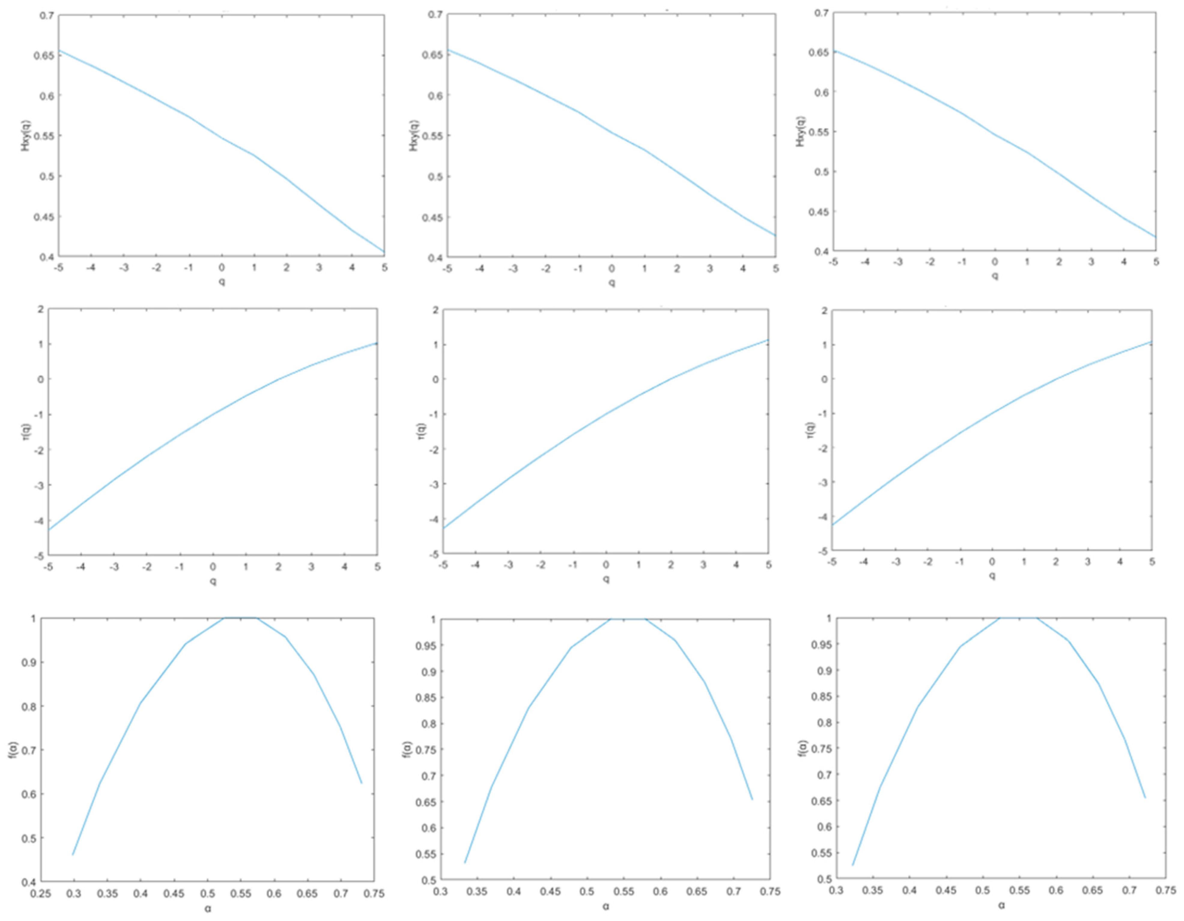
5.5. Robustness Tests

In this section, we employ another time window selected from 2005 to 2019 to conduct the MF-DFA and MF-DCCA analysis and obtain similar results.

Table 4. Multifractal properties of the returns of the U.S. stock market indices in specified time window.

Index	Δα	Δf	R
SPX	1.1719	1.3489	−0.3412
DJI	1.2672	1.6787	−0.3553
IXIC	0.9365	0.7183	−0.1428

shows that the returns exhibit multifractal properties in the period we now consider.

In addition, we use this time window to examine the multifractal properties of cross-correlations among the returns. The results are similar to those we have obtained in this section. The multifractal properties of cross-correlations are shown in Figure 7.

6. Conclusions

This study investigates the multifractal properties of the returns in the U.S. stock market and the multifractal properties of cross-correlations among the series. According to analysis through the MF-DFA and MF-DCCA methods, there is evidence of multifractal properties of the returns and their cross-correlations. The asymmetrical multifractal properties and multifractal cross-correlations in the U.S. stock market may contribute to a complex nonlinear system.

Main conclusions are as follows. First, for the whole sample, the SPX exhibits the highest multifractal degree, while the DJI exhibits the lowest multifractal degree. This means that the SPX has comparatively larger volatility. Second, the cross-correlation between the SPX and the DJI has the greatest multifractal level among the three pairs of the returns. This indicates the largest volatility in the return cross-correlation. Third, for the three pairs of indices, the cross-correlated behaviors of small fluctuations are more persistent than those of large fluctuations. Finally, the U.S. stock market exhibits asymmetrical multifractal properties, which implies different multifractal properties in different stages. The multifractal properties are different during downward and upward trends in the market. The returns considered show lower multifractal degrees under a downward trend of prices than under an upward trend. The SPX has the highest multifractal degree when the upward trend occurs, whereas the IXIC has the lowest multifractal degree. The DJI has the highest multifractal degree when the downward trend occurs, whereas the IXIC still has the lowest multifractal degree. The SPX experiences the greatest fluctuations when the market witnesses a shift from a downward trend to an upward trend. Regarding multifractal properties, the SPX demonstrates greater differences and volatilities during different market periods.

These empirical results reveal important implications for different entities in the U.S. stock market. For investors, they may respond to the market information in a nonlinear way and should comprehensively consider the stock market as a whole and take into account the impacts of fluctuations in different returns on future returns to effectively manage the portfolio risks. For policy makers and regulators, they may continue to monitor the risks and abnormalities in the market and promote the healthy development of the market.

More studies will be conducted to uncover the determinants of the inefficiency and cross-correlations in the U.S. stock market dynamics. In the subsequent research, we will discuss more about the impacts of trading strategies on the market and the dynamic cross-correlations in the market to develop a more comprehensive theoretical framework for the link of the multifractal properties to the efficiency and microstructure of the market. Moreover, we will study the issue of data quality and preprocessing in more depth.

References

1. Mandelbrot, B.B. A multifractal walk down wall street. Sci. Am. 1999, 280, 70–73. [Google Scholar] [CrossRef]
2. Peters, E.E. Fractal Market Analysis: Applying Chaos Theory to Investment and Economics; John Wiley Sons: New York, NY, USA, 1994; Volume 24. [Google Scholar]
3. Seth, N.; Sharma, A.K. International stock market efficiency and integration: Evidences from Asian and U.S. markets. J. Adv. Manag. Res. 2015, 12, 88–106. [Google Scholar] [CrossRef]
4. Ito, M.; Noda, A.; Wada, T. The Evolution of Stock Market Efficiency in the U.S.: A Non-Bayesian Time-Varying Model Approach. Appl. Econ. 2016, 48, 621–635. [Google Scholar] [CrossRef]
5. Benkraiem, R.; Lahiani, A.; Miloudi, A.; Shahbaz, M. New insights into the U.S. stock market reactions to energy price shocks. J. Int. Financ. Mark. Inst. Money 2018, 56, 169–187. [Google Scholar] [CrossRef]
6. Kyle, A.S.; Obizhaeva, A.A.; Tuzun, T. Microstructure invariance in U.S. stock market trades. J. Financ. Mark. 2020, 49, 100513. [Google Scholar] [CrossRef]
7. Oleg, S.; Grigory, P.; Alexander, S.; Sergiy, B.; Alexander, V.; Eduardo, L.P.; Vladimir, B. Networks of causal relationships in the U.S. stock market. Depend. Model. 2022, 10, 177–190. [Google Scholar]
8. Beckmann, L.; Debener, J.; Hark, P.F.; Pfingsten, A. CBDC and the shadow of bank disintermediation: US stock market insights on threats and remedies. Financ. Res. Lett. 2024, 67, 105868. [Google Scholar] [CrossRef]
9. Ammy-Driss, A.; Garcin, M. Efficiency of the financial markets during the COVID-19 crisis: Time-varying parameters of fractional stable dynamics. Phys. A Stat. Mech. Its Appl. 2023, 609, 128335. [Google Scholar] [CrossRef]
10. Belhoula, M.M.; Mensi, W.; Al Yahyaee, K.H. Dynamic speculation and efficiency in European natural gas markets during the COVID-19 and Russia-Ukraine crises. Resour. Policy 2024, 98, 105362. [Google Scholar] [CrossRef]
11. Sharif, T.; Ghouli, J.; Bouteska, A.; Abedin, M.Z. The impact of COVID-19 uncertainties on energy market volatility: Evidence from the US markets. Econ. Anal. Policy 2024, 84, 25–41. [Google Scholar] [CrossRef]
12. Koangsung, C.; Francesco, R.; Chung, C. The impact of COVID-19 on the Korean and US labour markets. Appl. Econ. 2024, 56, 4529–4543. [Google Scholar]
13. Benjamin, C.; Martin, H.; Kai, Z. The Impact of High-Frequency Trading on Modern Securities Markets. Bus. Inf. Syst. Eng. 2022, 65, 7–24. [Google Scholar]
14. Inés, J.; Andrés, M.-V.; Javier, P. Multivariate dynamics between emerging markets and digital asset markets: An application of the SNP-DCC model. Emerg. Mark. Rev. 2023, 56, 101054. [Google Scholar]
15. Kocaarslan, B. Dynamic spillovers between oil market, monetary policy, and exchange rate dynamics in the US. Financ. Res. Lett. 2024, 69, 106137. [Google Scholar] [CrossRef]
16. Shaw, P.K.; Saha, D.; Ghosh, S.; Janaki, M.S.; Iyengar, A.N.S. Investigation of multifractal nature of floating potential fluctuations obtained from a dc glow discharge magnetized plasma. Phys. A Stat. Mech. Its Appl. 2017, 469, 363–371. [Google Scholar] [CrossRef]
17. Al-Yahyaee, K.H.; Mensi, W.; Yoon, S.M. Efficiency; multifractality, and the long-memory property of the Bitcoin market: A comparative analysis with stock, currency, and gold markets. Financ. Res. Lett. 2018, 27, 228–234. [Google Scholar] [CrossRef]
18. Stosic, D.; Stosic, D.; de Mattos Neto, P.S.; Stosic, T. Multifractal characterization of Brazilian market sectors. Phys. A Stat. Mech. Its Appl. 2019, 525, 956–964. [Google Scholar] [CrossRef]
19. Tiwari, A.K.; Aye, G.C.; Gupta, R. Stock market efficiency analysis using long spans of Data: A multifractal detrended fluctuation approach. Financ. Res. Lett. 2019, 28, 398–411. [Google Scholar] [CrossRef]
20. Wang, F.; Ye, X.; Wu, C. Multifractal characteristics analysis of crude oil futures prices fluctuation in China. Phys. A Stat. Mech. Its Appl. 2019, 533, 122021. [Google Scholar] [CrossRef]
21. Mensi, W.; Kumar, A.S.; Vo, X.V.; Kang, S.H. Asymmetric multifractality and dynamic efficiency in DeFi markets. J. Econ. Financ. 2023, 48, 280–297. [Google Scholar] [CrossRef]
22. de Salis, E.A.; dos Santos Maciel, L. How does price (in)efficiency influence cryptocurrency portfolios performance? The role of multifractality. Quant. Financ. 2023, 23, 1637–1658. [Google Scholar] [CrossRef]
23. Li, W.; Lu, X.; Ren, Y.; Zhou, Y. Dynamic relationship between RMB exchange rate index and stock market liquidity: A new perspective based on MF-DCCA. Phys. A Stat. Mech. Its Appl. 2018, 508, 726–739. [Google Scholar] [CrossRef]
24. Zhang, W.; Wang, P.; Li, X.; Shen, D. The inefficiency of cryptocurrency and its cross-correlation with Dow Jones Industrial Average. Phys. A Stat. Mech. Its Appl. 2018, 510, 658–670. [Google Scholar] [CrossRef]
25. Ruan, Q.; Yang, B.; Ma, G. Detrended cross-correlation analysis on RMB exchange rate and Hang Seng China Enterprises Index. Phys. A Stat. Mech. Its Appl. 2017, 468, 91–108. [Google Scholar] [CrossRef]
26. Fang, S.; Lu, X.; Li, J.; Qu, L. Multifractal detrended cross-correlation analysis of carbon emission allowance and stock returns. Phys. A Stat. Mech. Its Appl. 2018, 509, 551–566. [Google Scholar] [CrossRef]
27. Ghosh, D.; Chakraborty, S.; Samanta, S. Study of translational effect in Tagore’s Gitanjali using Chaos based Multifractal analysis technique. Phys. A Stat. Mech. Its Appl. 2019, 523, 1343–1354. [Google Scholar] [CrossRef]
28. Ahmed, H.; Aslam, F.; Ferreira, P. Navigating Choppy Waters: Interplay between Financial Stress and Commodity Market Indices. Fractal Fract. 2024, 8, 96–118. [Google Scholar] [CrossRef]
29. Kantelhardt, J.W.; Zschiegner, S.A.; Koscielny-Bunde, E.; Havlin, S.; Bunde, A.; Stanley, H.E. Multifractal detrended fluctuation analysis of nonstationary time series. Phys. A Stat. Mech. Its Appl. 2002, 316, 87–114. [Google Scholar] [CrossRef]
30. He, L.-Y.; Chen, S.-P. Are crude oil markets multifractal? Evidence from MF-DFA and MF-SSA perspectives. Phys. A Stat. Mech. Its Appl. 2010, 389, 3218–3229. [Google Scholar] [CrossRef]
31. Alvarez-Ramirez, J.; Cisneros, M.; Ibarra-Valdez, C.; Soriano, A. Multifractal Hurst analysis of crude oil prices. Phys. A Stat. Mech. Its Appl. 2002, 313, 651–670. [Google Scholar] [CrossRef]
32. Cao, G.; Cao, J.; Xu, L. Asymmetric multifractal scaling behavior in the Chinese stock market: Based on asymmetric MF-DFA. Phys. A Stat. Mech. Its Appl. 2013, 392, 797–807. [Google Scholar] [CrossRef]
33. Onali, E.; Goddard, J. Unifractality and multifractality in the Italian stock market. Int. Rev. Financ. Anal. 2009, 18, 154–163. [Google Scholar] [CrossRef]
34. Wang, Y.; Wu, C.; Pan, Z. Multifractal detrending moving average analysis on the U.S. Dollar exchange rates. Phys. A Stat. Mech. Its Appl. 2011, 390, 3512–3523. [Google Scholar] [CrossRef]
35. Ning, Y.; Wang, Y.; Yang, Z.; Geng, Y. Measurement and multifractal properties of short-term international capital flows in China. Phys. A Stat. Mech. Its Appl. 2017, 468, 714–721. [Google Scholar] [CrossRef]
36. Ihlen, E.A.F. Introduction to multifractal detrended fluctuation analysis in Matlab. Front. Physiol. 2012, 3, 141. [Google Scholar] [CrossRef] [PubMed]
37. Zhou, W. Multifractal detrended cross-correlation analysis for two nonstationary signals. Phys. Rev. E 2008, 77, 066211. [Google Scholar] [CrossRef]
38. He, L.-Y.; Chen, S.-P. Nonlinear bivariate dependency of price–volume relationships in agricultural commodity futures markets: A perspective from multifractal detrended cross-correlation analysis. Phys. A Stat. Mech. Its Appl. 2011, 390, 297–308. [Google Scholar] [CrossRef]
39. Zhu, P.; Tang, Y.; Wei, Y.; Dai, Y. Portfolio strategy of international crude oil markets: A study based on multiwavelet denoising-integration MF-DCCA method. Phys. A Stat. Mech. Its Appl. 2019, 535, 122515. [Google Scholar] [CrossRef]
40. Yuan, Y.; Zhuang, X.-T.; Liu, Z.-Y. Price–volume multifractal analysis and its application in Chinese stock markets. Phys. A Stat. Mech. Its Appl. 2012, 391, 3484–3495. [Google Scholar] [CrossRef]
41. Cao, G.; Zhang, M.; Li, Q. Volatility-constrained multifractal detrended cross-correlation analysis: Cross-correlation among Mainland China, US, and Hong Kong stock markets. Phys. A Stat. Mech. Its Appl. 2017, 472, 67–76. [Google Scholar] [CrossRef]
Figure 1. Prices and returns of the U.S. stock market indices. Notes: “SPX”, “DJI”, and “IXIC” denote the daily returns of the Standard and Poor’s 500, the Dow Jones Industrial Average, and the Nasdaq Composite indices, respectively. “I” and “II” represent the sub-period 1 and sub-period 2, respectively. The green and red dashed lines describe the two sub-periods. Data source: Wind database.
Fractalfract 09 00073 g001
Figure 2. The Hurst exponent and multifractal spectrum of the daily returns. Notes: “SPX”, “DJI”, and “IXIC” denote the returns of the Standard and Poor’s 500 Index, the Dow Jones Industrial Average, and the Nasdaq Composite Index, respectively. Figure 2 describes the Hurst exponent and multifractal spectrum of the SPX, DJI, and IXIC indices, respectively. q, H(q), hq, and Dq denote order value, q-order Hurst exponent, singularity strength, and singularity spectrum, respectively.
Fractalfract 09 00073 g002
Figure 3. Hxy(q) value with q varying from −5 to 5 for each bivariate case of SPX, DJI, and IXIC. Notes: “SPX”, “DJI”, and “IXIC” denote the returns of the Standard and Poor’s 500 Index, the Dow Jones Industrial Average, and the Nasdaq Composite Index, respectively. q and Hxy(q) denote the order value and the generalized cross-correlation exponent, respectively.
Fractalfract 09 00073 g003
Figure 4. Plots of τ(q) versus q with q varying from −5 to 5 for each bivariate case of the returns. Notes: “SPX”, “DJI”, and “IXIC” denote the returns of the Standard and Poor’s 500 Index, the Dow Jones Industrial Average and the Nasdaq Composite Index, respectively. q and τ(q) denote the order value and the Renyi exponent, respectively.
Fractalfract 09 00073 g004
Figure 5. Multifractal spectrum of the cross-correlations with q varying from 5 to −5 for each bivariate case of the returns. Notes: “SPX”, “DJI”, and “IXIC” denote the returns of the Standard and Poor’s 500 Index, the Dow Jones Industrial Average and the Nasdaq Composite Index, respectively. α and f (α) denote the singularity exponent and the multifractal spectrum of the cross-correlations, espectively.
Fractalfract 09 00073 g005
Figure 6. Log–log plots of Fq(s) versus s with q varying from −5 to 5 for each bivariate case of the returns. Notes: “SPX”, “DJI”, and “IXIC” denote the returns of the Standard and Poor’s 500 Index, the Dow Jones Industrial Average and the Nasdaq Composite Index, respectively. Curves from the bottom to the top are corresponding to the plots with q = −5, −4, …, 4, 5.
Fractalfract 09 00073 g006
Figure 7. The multifractal properties of cross-correlations for each bivariate case of the returns. Notes: Each set of figures represents SPX-DJI, SPX-IXIC, and DJI-IXIC from left to right.
Fractalfract 09 00073 g007aFractalfract 09 00073 g007b