Fractional Calculus of Piecewise Continuous Functions

Abstract

The fractional derivative computation of piecewise continuous functions is treated with generality. It is shown why some applications give incorrect results and why Caputo derivative give strange results. Some examples are described.

1. Introduction

Mathematics is a free construction of the human mind that does not obey external rules. Perhaps strangely, some of the mathematical constructions are useful for the development of Science and Engineering. This means that it is not to be expected that all the operators and results obtained will be of interest in those areas. It is they who, on the basis of experimental results, select the operators and techniques that really matter. Often, it is researchers in these areas who introduce and develop these mathematical techniques. This may mean that there should be a distinction, albeit not a very clear one, between applications of mathematics, such as signal processing [1,2] and applied mathematics. Such a distinction was highlighted by D. Wilson a few years ago [3].

Entering Fractional Calculus, we find a huge number of derivatives and pseudo-derivatives that produce great confusion in the minds of those who just want to apply some of these derivatives to practical problems [4,5,6,7,8,9,10]. Some work on unification and synthesis has been done, but it cannot be said that it has been successful [11,12,13,14]. In everyday mathematics, there are operators who, for some particular reason, become famous and fashionable. This is often because they introduce some simplification into the calculation. However, nobody said that Nature is simple. Therefore, it is not expectable they are very useful.

Therefore, it is important to select those derivatives that are suitable for being used in Sciece and Engineering for modelling/identification systems. It is important not to mix, without justification, different types of derivatives, as scale and shift invariant [15]. However, we need to find criteria for doing it. For now, we can state that such operators must:

• have back-compatibility with classic (integer order) formulations;
• be shift or scale invariant, since these are important characteristics of many physical, biologic, and social systems;
• be defined for as many as possible functions, avoiding particular features;
• be coherent with auxiliary mathematical tools, e.g., Laplace (bilateral) or Mellin transforms;
• transform a sinusoid into a sinusoid;
• have inverse, even if distribution theory has to be used, a very current situation in Physics and Engineering.

Usually, these rules are disregarded and supposedly simpler operators are adopted, leading to strange situations that give fractional calculus a bad name. It is well known the designation “metaphysical derivatives” associated to the fractional derivatives [16,17]. It is not difficult to see that such designation corresponds to partial observation of the correct results. The Riemann-Liouville (RL) and Caputo (C) derivatives are in this kind of situation, with the aggravating factor that they are the most commonly used derivatives in milliards of books and papers. Some years ago [18] we made an analysis of the main problems created by RL and C derivatives and showed they have several shortcomings:

• They make a confusion between the constant function $f\left(t\right)=1$ and the Heaviside unit step;
• With the bad help of the one-sided Laplace transform, introduce wrong initial-conditions (these depend on the past history of the system and on its structure, not on any mathematical tool; the C initial-conditions are not good because they have integer order [19];
• Their derivatives of a sinusoid is not a sinusoid, preventing the correct definition of frequency response;
• They do not have additivity/commutativity of the orders which transforms an invariant system in variable.

Meanwhile, some reports of incorrect results were published, describing contradictions between theoretical and experimental results [20,21,22,23,24,25]. A recent paper [26] description and solution of several problems found in dealing with fractional calculus of piecewise continuous functions gave some motivation for this text. Several difficulties associated with the C, and also RL, were illustrated through several simple examples. In particular, it was shown that “additivity of integration on intervals for integer-order integral does not hold for fractional integrals, not to mention fractional derivatives”. In a similar way, the paper [27] shows some of the difficulties in computing the fractional derivatives of power functions.

Here, we will show that such difficulties are false problems and have simple solutions. All the difficulties have origins in the definitions and uses of fractional derivatives. In fact, the most used definitions are particularised in the sense that each derivative has its own definition, instead of having general definitions. This fact is easily understood by looking into the RL and Caputo derivative definitions [28,29,30]

$${}_{a }{}^{RL}D_t^{\alpha }f\left(t\right)={\displaystyle \frac{1}{\Gamma (n-\alpha )}}{\displaystyle \frac{d^n}{d{t}^n}}{\int }_{t_0}^t{\displaystyle \frac{f\left(\tau \right)}{{(t-\tau )}^{1+\alpha -n}}}\mathrm{d}\tau ,$$

(1)

and

$${}_a{}^{C}D_t^{\alpha }f\left(t\right)={\displaystyle \frac{1}{\Gamma (n-\alpha )}}{\int }_{t_0}^t{\displaystyle \frac{f^{\left(n\right)}\left(\tau \right)}{{(t-\tau )}^{1+\alpha -n}}}\mathrm{d}\tau ,$$

(2)

where $n-1<\alpha \le n,n\in {\mathbb{Z}}^{+}$ and $t\in [a,b]$. These derivatives impose a particular domain and a given “starting point”: each function has its own derivative definition. This creates difficulties when trying to deal with functions having different domains, so different definitions [26,31]. It is this problem that gives “justification” for the “metaphysical” character of some derivatives.

In this paper, we state that all the described problems are fictitious and disappear if we consider that all the functions are defined on $\mathbb{R}$. This is valid for any of the usual shift-invariant derivatives [11].

In the following, we will consider the problems described in [26] and present a new perspective into the solution. For reasons stated in [32], we will use the bilateral Laplace transform (LT). We will consider fractional derivatives with LT given by [32]

$$\mathcal{L}\left[D^{\alpha }f\left(t\right)\right]=s^{\alpha }\mathcal{L}\left[f\left(t\right)\right].$$

(3)

for $Re\left(s\right)\ge 0,s\ne 0.$ The paper outlines as follows. In Section 2 we introduce the shift-invariant (Duhamel) convolution and describe its properties (Section 2.1). The convolution of piecewise continuous function is treated in Section 2.2. In Section 3 we introduce the derivatives suitable for our study. These are used in Section 4 for exemplifying the applications to piecewise functions. Finally, we present some conclusions.

2. The Duhamel Convolution

2.1. Properties

Definition 1. 

Let $f\left(t\right)$ and $h\left(t\right)$ be two locally integrable functions with support on $\mathbb{R}$. We define the continuous-time Duhamel convolution as the operator given by [33,34,35,36]

$$g\left(t\right)=h\left(t\right)\ast f\left(t\right)={\int }_{-\infty }^{\infty }h\left(\tau \right)f(t-\tau )d\tau ={\int }_{-\infty }^{\infty }h(t-\tau )f\left(\tau \right)d\tau .$$

(4)

Working in the context of the distribution theory, we enlarge the validity of the above definition [37,38,39]. Assume also that $f\left(t\right)$ and $h\left(t\right)$ are of exponential order. We can prove that:

• The eigenfunction of the convolution is the exponential, $e^{st},s\in \mathbb{C},t\in \mathbb{R}$.
• The eigenvalue, $H\left(s\right)$, is given by

  $$H\left(s\right)={\int }_{-\infty }^{\infty }h\left(t\right)e^{-st}dt,$$

  (5)

  that is the bilateral Laplace transform (LT) [32]. In many interesting situations, the region of convergence (ROC), $\mathcal{R}$ [32] is a vertical strip that includes the imaginary axis, therefore $h\left(t\right)$ has Fourier transform.

The main properties of the convolution are [40]

• Commutativity

  $$h\left(t\right)\ast f\left(t\right)=f\left(t\right)\ast h\left(t\right);$$
• Associativity

  $$h\left(t\right)\ast f\left(t\right)\ast g\left(t\right)=\left(h\left(t\right)\ast f\left(t\right)\right)\ast g\left(t\right)=h\left(t\right)\ast \left(f\left(t\right)\ast g\left(t\right)\right);$$
• Invertibility

  $$h\left(t\right)\ast f^{-1}\left(t\right)=\delta \left(t\right);$$
• Neutral element

  $$h\left(t\right)\ast \delta \left(t\right)=h\left(t\right);$$
• Causality
  If $h\left(t\right)=0,t<0$, then

  $$g\left(t\right)={\int }_0^{\infty }h\left(\tau \right)f(t-\tau )d\tau ={\int }_{-\infty }^{t}h(t-\tau )f\left(\tau \right)d\tau .$$

  (6)
  It means that the output $g\left(t\right)$ at a given $t=t_0$ depends only on the values of $f\left(t\right)$ for $t\le t_0.$ In the following, we shall be dealing with this case.
• Shifting

  $$g\left(t\right)=h\left(t\right)\ast f\left(t\right)\to h(t-a)\ast f(t-b)=g(t-a-b);$$

  (7)
• Derivation

  $${\displaystyle \frac{d}{dt}}\left(h\left(t\right)\ast f\left(t\right)\right)=\left({\displaystyle \frac{dh\left(t\right)}{dt}}\ast f\left(t\right)\right)$$

  (8)

Remark 1. 

This last property deserves some comments since it is very important [41].

• Due to the commutativity, we can choose which is the more suitable function to be differentiated;
• It is known that the result of the convolution is a smoother function than each of the factors;
• Attending to the previous statement, it is clear that the existence of the right hand side implies the existence of the left one, but the reverse may not be true;
• For functions with LT, they are equal.

2.2. Bounded Piecewise Continuous Functions

Definition 2. 

Let N be a positive integer number. Consider a bounded function defined on $\mathbb{R}$ by

$$f\left(t\right)=\left\{\begin{array}{cc}{f}_0\left(t\right)\hfill & t<t_0\hfill \\ \cdots \hfill & \hfill \\ f_k\left(t\right)\hfill & t_k<t<t_{k+1},k=1,\cdots ,N-1\hfill \\ \cdots \hfill & \hfill \\ f_N\left(t\right)\hfill & t>t_N\hfill \end{array}\right.$$

(9)

where all the involved functions are continuous and have bounded variation. $f\left(t\right)$ is a bounded piecewise continuous function.

This definition can be extended to include periodic and almost periodic functions.

Let $h\left(t\right)$ be the impulse response of a causal linear system described by (6), but suppose that $f\left(t\right),t\in \mathbb{R}$ assumes several forms, particular cases of piecewise continuous function.

• Let $f\left(t\right),t\in \mathbb{R}$ be a bounded support function (BSF)

  $$f\left(t\right)=\left\{\begin{array}{cc}{f}_0\left(t\right)\hfill & t_0<t<t_1\hfill \\ 0\hfill & t<t_0\wedge t>t_1\hfill \end{array}\right..$$

  The corresponding output is given by

  $$g\left(t\right)=\left\{\begin{array}{cc}0\hfill & t<t_0\hfill \\ {\int }_{t_0}^{min(t,t_1)}h(t-\tau )f_0\left(\tau \right)d\tau \hfill & t>t_0.\hfill \end{array}\right.$$

  (10)

  This means that, even the input has finite duration, the output has an infinite support. For simplicity, we will assume by default that the convolution exists but is null for values of t less than the lower limit of the integral.

  Example 1. 

  Let

  $$h\left(t\right)=t^{\alpha -1}\epsilon \left(t\right)$$

  where $\alpha >0$ and $\epsilon \left(t\right)$ is the Heaviside function. Assume that $f\left(t\right)$ a is rectangular pulse

  $$f\left(t\right)=\epsilon (t+1)-\epsilon (t-1).$$

  The convolution gives

  $$g\left(t\right)={\int }_{-1}^{min(t,1)}{(t-\tau )}^{\alpha -1}d\tau ={\displaystyle \frac{1}{\alpha }}\left\{\begin{array}{cc}{(t+1)}^{\alpha }\hfill & -1<t<1\hfill \\ {(t+1)}^{\alpha }-{(t-1)}^{\alpha }\hfill & t\ge 1\hfill \end{array}\right..$$

  (11)
• Consider two BSF, $f_0\left(t\right)$, as above, and $f_1\left(t\right),t_2<t<t_3.$ For simplicity, set $t_0<t_2<t_1<t_3.$ We have

  $$g_0\left(t\right)={\int }_{t_0}^{min(t,t_1)}h(t-\tau )f_0\left(\tau \right)d\tau .$$

  and

  $$g_1\left(t\right)={\int }_{t_2}^{min(t,t_3)}h(t-\tau )f_1\left(\tau \right)d\tau .$$

  so that $g\left(t\right)=g_0\left(t\right)+g_1\left(t\right)$ is given by

  $$g\left(t\right)=\left\{\begin{array}{cc}{\int }_{t_0}^{min(t,t_2)}h(t-\tau )f_0\left(\tau \right)d\tau \hfill & t_0<t<t_2\hfill \\ {\int }_{t_0}^{t_2}h(t-\tau )f_0\left(\tau \right)d\tau +{\int }_{t_2}^{min(t,t_1)}h(t-\tau )\left[f_0\left(\tau \right)+f_1\left(\tau \right)\right]d\tau \hfill & t_2<t<t_1\hfill \\ {\int }_{t_0}^{t_1}h(t-\tau )f_0\left(\tau \right)d\tau +{\int }_{t_2}^{t_1}h(t-\tau )f_1\left(\tau \right)d\tau +{\int }_{t_2}^{min(t,t_3)}h(t-\tau )f_1\left(\tau \right)d\tau \hfill & t>t_1.\hfill \end{array}\right..$$

  Attending to the fact that

  $$f\left(t\right)=\left\{\begin{array}{cc}{f}_0\left(t\right)\hfill & t_0<t<t_2\hfill \\ f_0\left(t\right)+f_1\left(t\right)\hfill & t_2<t<t_1\hfill \\ f_1\left(t\right)\hfill & t_1<t<t_3.\hfill \end{array}\right.,$$

  we can show the validity of the additivity property. With some interest in applications is the case $t_1=t_2$ (disjoint supports). In this case,

  $$g\left(t\right)=\left\{\begin{array}{cc}{\int }_{t_0}^{min(t,t_2)}h(t-\tau )f_0\left(\tau \right)d\tau \hfill & t_0<t<t_1\hfill \\ {\int }_{t_0}^{t_1}h(t-\tau )f_0\left(\tau \right)d\tau +{\int }_{t_1}^{min(t,t_3)}h(t-\tau )f_1\left(\tau \right)d\tau \hfill & t>t_1.\hfill \end{array}\right.=g_0\left(t\right)+g_1\left(t\right).$$

  (12)

  In the general case stated in Definition 2 and for a given $t_K<t<t_{K+1}$ we obtain

  $$\begin{array}{cc}\hfill g\left(t\right)& =\sum _{m=0}^{K-1}{\int }_{t_m}^{t_{m+1}}h(t-\tau )f_m\left(\tau \right)d\tau +{\int }_{t_K}^{min(t,t_{K+1})}h(t-\tau )f_K\left(\tau \right)d\tau \hfill \\ \hfill & =\sum _{m=0}^K{\int }_{t_m}^{min(t,t_{m+1})}h(t-\tau )f_m\left(\tau \right)d\tau \hfill \\ \hfill & =\sum _{m=0}^K{g}_m\left(t\right).\hfill \end{array}$$

  (13)

  Finally, for any $t\in \mathbb{R},$ we have

  $$g\left(t\right)=\sum _{m=0}^N{\int }_{t_m}^{min(t,t_{m+1})}h(t-\tau )f_m\left(\tau \right)d\tau$$

  (14)

We showed that the convolution of a BSF resulting from the concatenation of a given number of pieces is the sum of the partial convolutions.

• These results are useful in the computation of fractional derivatives.

3. Liouville Type Derivatives

3.1. Definitions

The idea of non integer order differentiation seems to have resulted from some reflections expressed by Leibniz in a letter addressed to J. Bernoulli [16]. The subject was first discussed between the two and later with other mathematicians, but no formula or procedure resulted. Euler, Abel, and Fourier touched the problem, but did not produce any developments. The first real important contribution in fractional calculus was accomplished by J. Liouville that proposed several formulae for computing the derivatives of any order [42,43,44]. However, Liouville based his theory on the development of the functions as a sum of exponentials, what created several technical dificulties because at that time the Bromwich integral was not yet formulated. Among several formulae he proposed generalizations of the incremental ratio. However, the importance of this result was overlooked and only later Grünwald and Letnikov returned to the subject, but considering only the particular case of functions defined in ${\mathbf{R}}^{+}$. The designation “Grünwald-Letnikov derivatives” is currently adopted in incremental ratio based derivatives. Let the function $f\left(t\right)$ to be defined on $\mathbf{R}$ and $\alpha$ any real number. We have the forward (causal) and backward (anti-causal) derivatives given by [43,45,46,47]:

$$D_f^{\alpha }f\left(t\right)=\underset{h\to 0^{+}}{lim}{\displaystyle \frac{{\displaystyle \sum _{n=0}^{\infty }}\frac{{(-\alpha )}_n}{n!}f(t-nh)}{h^{\alpha }}},$$

(15)

$$D_b^{\alpha }f\left(t\right)=e^{-i\pi \alpha }\underset{h\to 0^{+}}{lim}{\displaystyle \frac{{\displaystyle \sum _{n=0}^{\infty }}\frac{{(-\alpha )}_n}{n!}f(t+nh)}{h^{\alpha }}}.$$

(16)

In the following, we will treat the causal case only.

Example 2. 

Consider the constant function $f\left(t\right)=1,t\in \mathbb{R}$. For every $\alpha \in \mathbf{R}$, then we have

$$\begin{array}{c}\hfill D^{\alpha }f\left(t\right)=\underset{h\to 0^{+}}{lim}{\displaystyle \frac{{\sum }_{k=0}^{\infty }\left(\begin{array}{c}\alpha \\ k\end{array}\right){(-1)}^k}{h^{\alpha }}}=\left\{\begin{array}{cc}0,\hfill & \mathrm{if}\alpha >0\hfill \\ \hfill & \\ \infty ,\hfill & \mathrm{if}\alpha <0\hfill \end{array}\right..\end{array}$$

(17)

We can apply the two-sided LT to (15) to obtain (3)

$$\mathcal{L}\left[D_f^{\alpha }f\left(t\right)\right]=s^{\alpha }\mathcal{L}\left[f\left(t\right)\right],Re\left(s\right)>0.$$

We can use the convolution property of the LT, provided that we get the inverse LT of $s^{\alpha }$. We can show [48] that, if $\alpha >0,$

$${\mathcal{L}}^{-1}{\displaystyle \frac{1}{s^{\alpha }}}={\displaystyle \frac{t^{\alpha -1}}{\Gamma \left(\alpha \right)}}\epsilon \left(t\right).$$

(18)

Therefore, attending to (3), the fractional anti-derivative of $f\left(t\right)$ is given by a convolution

$$D^{-\alpha }f\left(t\right)={\displaystyle \frac{1}{\Gamma \left(\alpha \right)}}\underset{0}{\overset{\infty }{\int }}{\tau }^{\alpha -1}f(t-\tau )d\tau .$$

(19)

In the derivative case, the expression (19) is not as handy as (15), but it can be regularized [49]

$$D^{\alpha }f\left(t\right)={\displaystyle \frac{1}{\Gamma (-\alpha )}}\underset{0}{\overset{\infty }{\int }}{\tau }^{-\alpha -1}\left[f(t-\tau )-\sum _0^{N-1}{\displaystyle \frac{{(-1)}^m{f}^{\left(m\right)}\left(t\right)}{m!}}{\tau }^m\right]d\tau .$$

(20)

that we will call regularized Liouville derivative and where $N-1<\alpha \le N$. As $s^{\alpha }=s^N{s}^{\alpha -N}$, we can “transform” a derivative into a sequence of an anti-derivative and a classic derivative

$$\begin{array}{cc}\hfill D^{\alpha }f\left(t\right)& =D^N\left[{\displaystyle \frac{1}{\Gamma (-\alpha +N)}}\underset{0}{\overset{\infty }{\int }}{\tau }^{N-\alpha -1}f(t-\tau )d\tau \right]\hfill \\ \hfill & =D^N\left[{\displaystyle \frac{1}{\Gamma (-\alpha +N)}}\underset{-\infty }{\overset{t}{\int }}{(t-\tau )}^{N-\alpha -1}f\left(\tau \right)d\tau \right],\hfill \end{array}$$

(21)

that constitutes a derivative of the Riemann-Liouville type. Such derivative was introduced by Liouville and adopted by Weyl for studying the fractional calculus of sinusoids. Following Hilfer and Kleiner we will call it Liouville-Weyl derivative (LW) [13]. However, it appeared, for the first time, in the anti-causal version, in the first paper of Liouville [42,50]. The procedure makes sense, since it transfers the singularity to a pos-processing that consists in derivating a well-behaved function. However, we can consider the property of the convolution (8) and move the derivation to inside the convolution, $s^{\alpha }=s^{\alpha -N}{s}^N$.

$$D^{\alpha }f\left(t\right)={\displaystyle \frac{1}{\Gamma (-\alpha +N)}}\underset{-\infty }{\overset{t}{\int }}{(t-\tau )}^{N-\alpha -1}{f}^{\left(N\right)}d\tau .$$

(22)

This has been called Liouville-Caputo derivative [42,51]. However, in recent times, people attributed this designation to what has been called Caputo derivative. To be more clear, we will call it Liouville (L) derivative. It must be remarked that expression (22), while equivalent to (21) in terms of the LT, may be worse from analytical point of view, since successive derivations increase the rugosity. A fair comparison of the 3 derivatives lead us to conclude that

• If $f\left(t\right)$ has Laplace transform, the three derivatives give the same result;
• The Liouville derivative demands too much from analytical point of view, since it needs the existence of the $N^{th}$ order derivative, but this feature is interesting if the distributional environment is assumed;
• If $f\left(t\right)=1,t\in \mathbf{R}$ the Riemann-Liouville derivative does not exist, since the integral is divergent, the others give the correct result (17);
• The usual RL (1) and C (2) derivatives are particular cases of the LW and L derivatives.

3.2. The Constant Function vs. the Heaviside Unit Step

As written above, the RL and C derivatives make a confusion between the constant function $c\left(t\right)=1,t\in \mathbb{R}$ and the Heaviside unit step. While the RL gives a result that coincides with Liouville’s result, the C derivative gives the null function, a strange result that allows us the explain the abnormal results in laboratorial experiments [20,22,25].

The derivative of the constant function in the sense of Liouville is the null function, as shown above. Concerning the Heaviside function, we showed above for the GL derivative, that it is given by ${\displaystyle \frac{t^{-\alpha }}{\Gamma (1-\alpha )}}\epsilon \left(t\right)$. It is easy to prove it with the LR and L derivatives. For simplicity, let $0<\alpha <1$. We can show that [47]

$$D^{\alpha }\epsilon \left(t\right)={\displaystyle \frac{t^{-\alpha }}{\Gamma (1-\alpha )}}\epsilon \left(t\right).$$

(23)

This relation can be obtained from the three derivatives and enlarge its validity; for example:

$$D^{\alpha }\epsilon \left(t\right)={\displaystyle \frac{1}{\Gamma (-\alpha )}}\underset{-\infty }{\overset{t}{\int }}{(t-\tau )}^{-\alpha }\delta \left(\tau \right)d\tau ={\displaystyle \frac{t^{-\alpha }}{\Gamma (1-\alpha )}}$$

This last result enters in contradiction with the C solution which identifies the Heaviside function with a constant and gives a null value.

As $\delta \left(t\right)=Du\left(t\right)$, we have also

$$D^{\alpha }\delta \left(t\right)={\displaystyle \frac{t^{-\alpha -1}}{\Gamma (-\alpha )}}\epsilon \left(t\right).$$

(24)

Example 3. 

According to the above result, the fractional derivative of a rectangular pulse,

$$p\left(t\right)=\epsilon \left(t\right)-\epsilon (t-d),d\in \mathbb{R},$$

is

$$D^{\alpha }p\left(t\right)={\displaystyle \frac{t^{-\alpha }\epsilon \left(t\right)-{(t-d)}^{-\alpha }\epsilon (t-d)}{1-\alpha }}.$$

This is illustrated in Figure 1. It must be stressed the fact that for positive orders near 1 it is clear that the derivative approaches two impulses. This is a consequence of [37]

$${\displaystyle \frac{t^{-1}}{\Gamma \left(0\right)}}\epsilon \left(t\right)=\delta \left(t\right).$$

3.3. The Derivatives and the Convolution

The derivatives we introduced above are essentially convolutions. Therefore, the properties we described in Section 2.1 have direct application. For the BSF case, we must have in mind our conclusions presented in Section 2.2. In the anti-derivative case, we have direct application of the rules. For the Liouville-Weyl case, the situation is similar, since we have to make derivations after doing the convolution. As referred, this operation increases the smoothness of the function. This does not happen with the L derivative, since we are doing derivations of discontinuous functions. In such a situation, impulses and their derivatives will appear. We wonder why this does not happen with current uses of the C derivative. The reason is in the use of the one-sided LT that introduces (indirectly) a regularization and of the classic derivation rules. This explains why the C derivative of the Heaviside function is the null function, an abnormal result that implies that the derivative of the impulse is also null.

4. Illustrative Examples

4.1. Simple Differential Equations

Example 4. 

Consider the differential equation [26]

$$D^{\alpha }x\left(t\right)=\left\{\begin{array}{cc}-ax\left(t\right)\hfill & 0<t\le 1\hfill \\ 0\hfill & t>1,\hfill \end{array}\right.$$

(25)

where $\alpha >0$. To have non null solution we have to impose a given initial condition (IC), $x\left(0\right)=1$. To include such IC, we transform the differential equation into [19]

$$D^{\alpha }\left[x\left(t\right)-x\left(0\right)\epsilon \left(t\right)\right]=-ax\left(t\right),0<t\le 1,$$

where $\epsilon \left(t\right)$ is the Heaviside function and $a\in \mathbb{R}.$ Note that the subtraction in brackets is intended to remove the jump at the origin, since $x\left(t\right)=0,t<0$. Using the LT, we get

$$s^{\alpha }\left[X\left(s\right)-{\displaystyle \frac{x\left(0\right)}{s}}\right]=-aX\left(s\right),Re\left(s\right)>0.$$

Therefore,

$$X\left(s\right)={\displaystyle \frac{s^{\alpha -1}}{s^{\alpha }+a}},$$

which gives the solution ($x\left(0\right)=1$)

$$x\left(t\right)=\sum _{k=0}^{\infty }{(-a)}^k{\displaystyle \frac{t^{\alpha k}}{\Gamma (\alpha k+1)}},$$

that is the well-known Mittag-Leffler function. It is interesting to note that this corresponds to solving

$$D^{\alpha }x\left(t\right)+ax\left(t\right)=x\left(0\right){\displaystyle \frac{t^{-\alpha }}{\Gamma (-\alpha +1)}}\epsilon \left(t\right),0<t\le 1.$$

Now, we consider the computation of the solution for $t>1$. In this case, the IC is

$$x\left(1\right)=\sum _{k=0}^{\infty }{(-a)}^k{\displaystyle \frac{1}{\Gamma (\alpha k+1)}}.$$

If $a>0$ the convergence is fast. According to the above description, our problem can be rewritten as

$$D^{\alpha }\left[x\left(t\right)-x\left(1\right)\epsilon (t-1)\right]=0,t>1.$$

Therefore, the solution is obtained from the above result, by setting $a=0$ and introducing a shift

$$x\left(t\right)=x\left(1\right)\sum _{k=0}^{\infty }{(-a)}^k{\displaystyle \frac{t^{\alpha k}}{\Gamma (\alpha k+1)}}{\epsilon \left(t\right)|}_{a=0}=x\left(1\right)\epsilon (t-1).$$

These results are valid for any positive derivative orders and contradict the solution obtained in [26]. Besides, they express a coherence integer/fractional orders. Such facts are illustrated in Figure 2.

Example 5. 

Now, let $v\left(t\right)=t\left[\epsilon \right(t)-\epsilon (t-1\left)\right]$ that is the input to the following differential equation

$$D^{\alpha }x\left(t\right)=v\left(t\right).$$

We have two approaches to do it:

• Using the LT, we obtain easily

  $$s^{\alpha }X\left(s\right)=V\left(s\right).$$
  with $V\left(s\right)=\mathcal{L}v\left(t\right)$. As $v\left(t\right)=t\epsilon \left(t\right)-(t-1)\epsilon (t-1)-\epsilon (t-1)$,

  $$V\left(s\right)={\displaystyle \frac{1-e^{-s}}{s^2}}-{\displaystyle \frac{e^{-s}}{s}},Re\left(s\right)>0.$$
  So,

  $$X\left(s\right)={\displaystyle \frac{1-e^{-s}}{s^{2+\alpha }}}-{\displaystyle \frac{e^{-s}}{s^{1+\alpha }}},Re\left(s\right)>0,$$
  which leads to

  $$x\left(t\right)={\displaystyle \frac{t^{\alpha +1}}{\Gamma (\alpha +2)}}\epsilon \left(t\right)-{\displaystyle \frac{{(t-1)}^{\alpha +1}}{\Gamma (\alpha +2)}}\epsilon (t-1)-{\displaystyle \frac{{(t-1)}^{\alpha }}{\Gamma (\alpha +1)}}\epsilon (t-1)$$
• Directly

  $$x\left(t\right)=D^{-\alpha }v\left(t\right).$$
  Therefore,

  $$\begin{array}{cc}\hfill x\left(t\right)& ={\displaystyle \frac{1}{\Gamma \left(\alpha \right)}}{\int }_0^{min(t,1)}\tau {(t-\tau )}^{\alpha -1}d\tau \hfill \\ & ={\displaystyle \frac{1}{\Gamma \left(\alpha \right)}}\left\{\begin{array}{cc}{\int }_0^t\tau {(t-\tau )}^{\alpha -1}d\tau \hfill & 0<t<1\hfill \\ {\int }_0^1\tau {(t-\tau )}^{\alpha -1}d\tau \hfill & t>1.\hfill \end{array}\right.\hfill \\ & =\left\{\begin{array}{cc}{\displaystyle \frac{t^{\alpha +1}}{\Gamma (\alpha +2)}}\hfill & 0<t<1\hfill \\ -{\displaystyle \frac{{(t-1)}^{\alpha }}{\Gamma (\alpha +1)}}\epsilon (t-1)+{\displaystyle \frac{t^{\alpha +1}-{(t-1)}^{\alpha +1}}{\Gamma (\alpha +2)}}\epsilon (t-1)\hfill & t>1.\hfill \end{array}\right.\hfill \end{array}$$

This solution is depicted for several values of α in Figure 3.

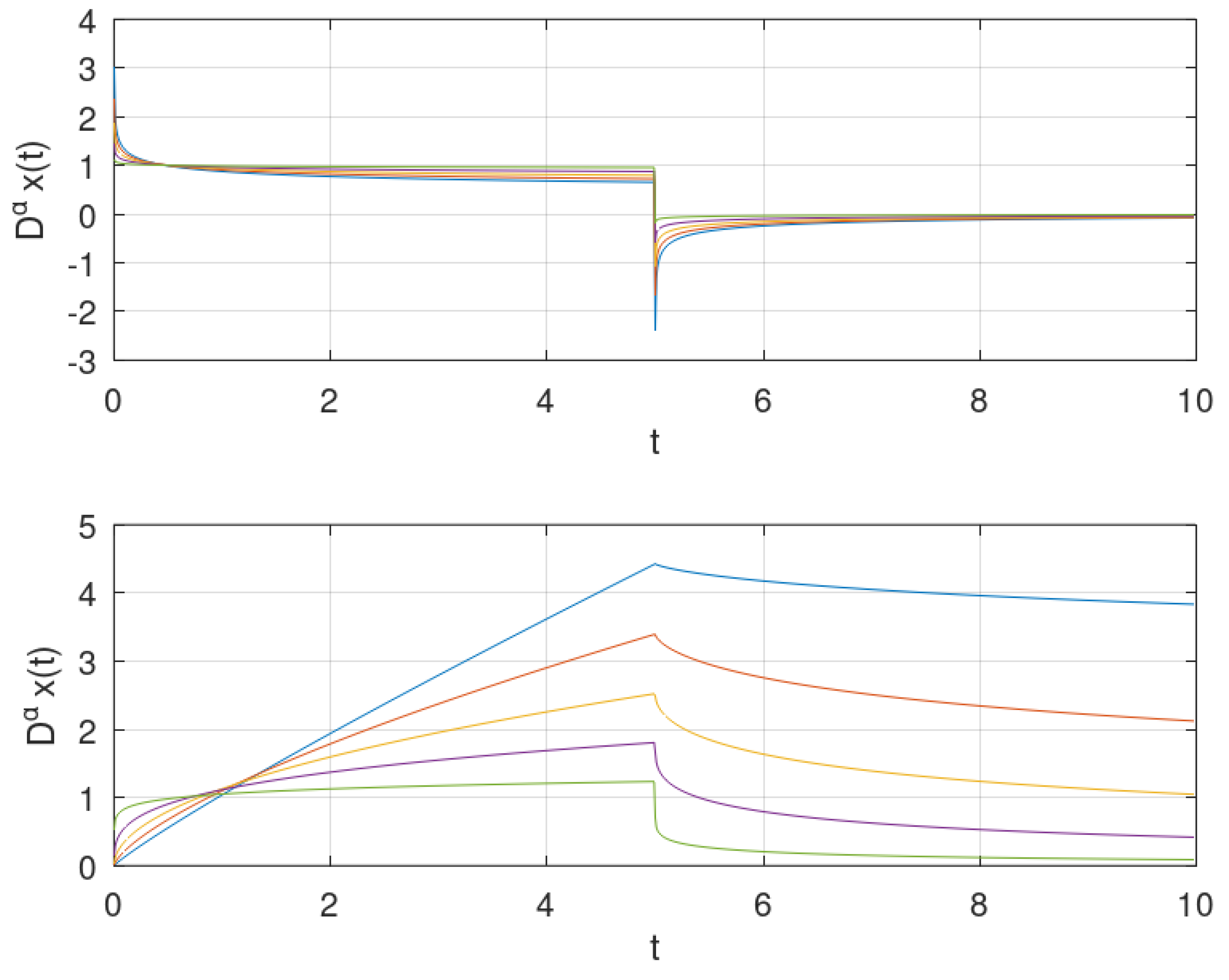
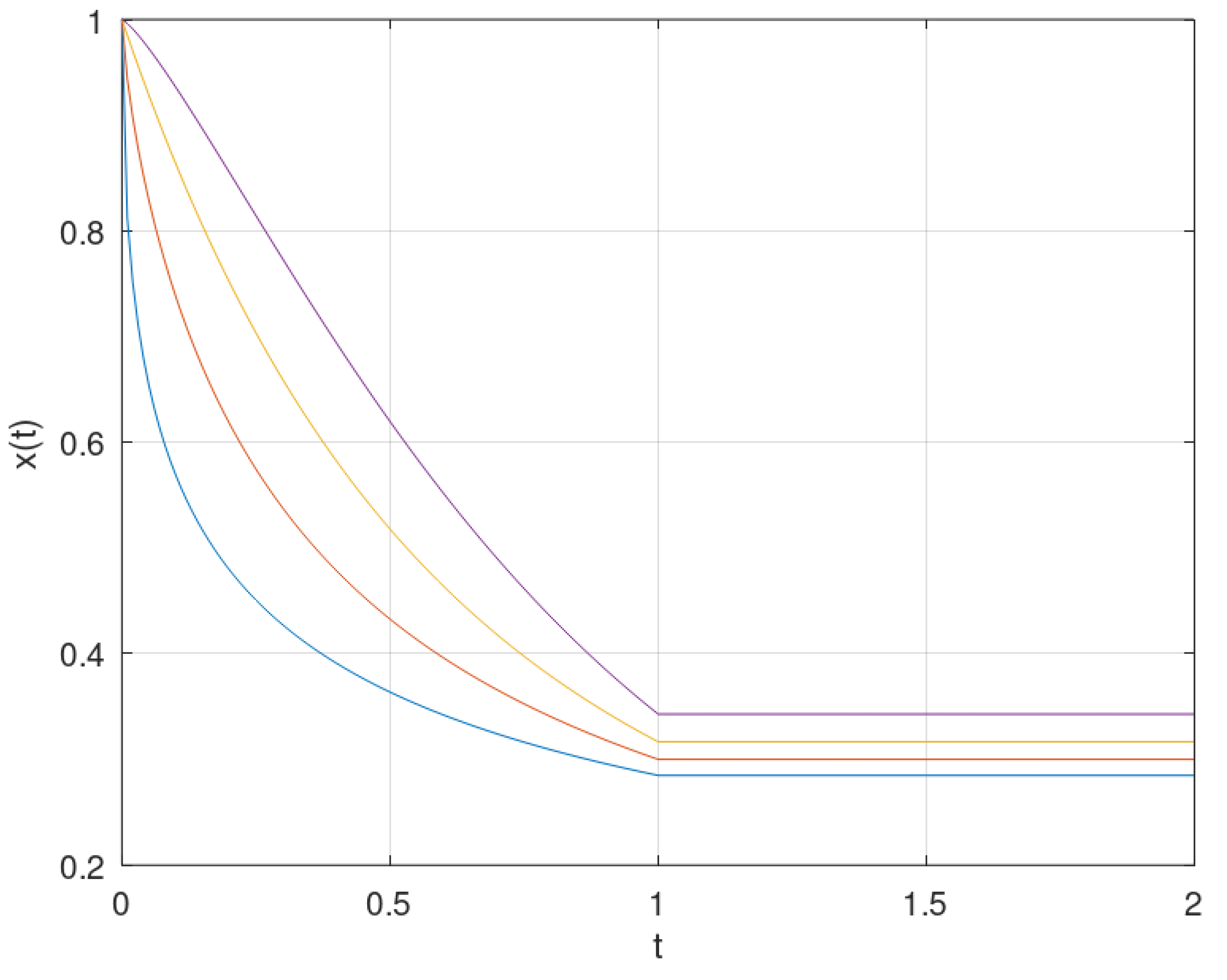
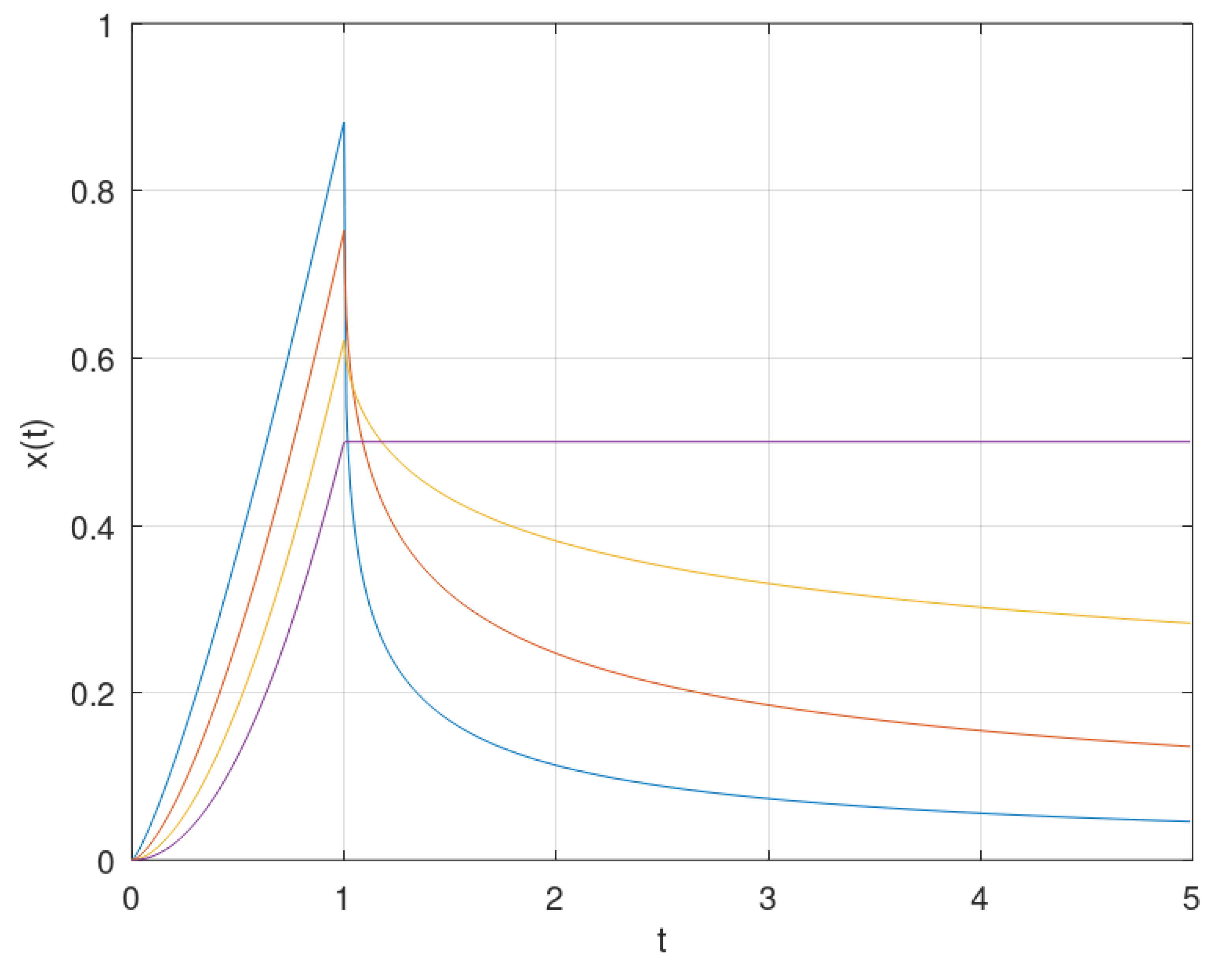
4.2. Concatenated Bounded Continuous Functions

Consider a bounded function defined in Section 2.

Theorem 1. 

The Liouville derivative of the $k^{th}$ function, $f_k\left(t\right),$ is given by

$${}^{L}D_t^{\alpha }{f}_k\left(t\right)=\left\{\begin{array}{cc}0\hfill & t<t_k\hfill \\ {\displaystyle \frac{1}{\Gamma (n-\alpha )}}{\int }_{t_k}^{min(t,t_{k+1})}{\displaystyle \frac{f_k^{\left(n\right)}\left(\tau \right)}{{(t-\tau )}^{1+\alpha -n}}}\mathrm{d}\tau \hfill & t>t_k.\hfill \end{array}\right.$$

(26)

The proof is obvious. It is important to highlight the fact that, while the function is of bounded support, the derivative is not. On the other hand, the derivative must be taken in generalized sense, to keep the coherence with the bilateral LT. We will continue with the L derivative, since it is the one that creates more difficulties (we remove the “L”).

According to the previous theorem, we can say that the derivative of a sum is the sum of the derivatives, but we must be careful with the range of the derivative.

Corollary 1. 

Let

$$g\left(t\right)=\left\{\begin{array}{cc}{f}_0\left(t\right)\hfill & t<t_1\hfill \\ f_1\left(t\right)\hfill & t_1<t<t_2\hfill \end{array}\right.$$

We have

$$D_t^{\alpha }g\left(t\right)={\displaystyle \frac{1}{\Gamma (n-\alpha )}}{\int }_{-\infty }^{min(t,t_2)}{\displaystyle \frac{f_0^{\left(n\right)}\left(\tau \right)+f_1^{\left(n\right)}\left(\tau \right)}{{(t-\tau )}^{1+\alpha -n}}}\mathrm{d}\tau$$

$$D_t^{\alpha }g\left(t\right)={\displaystyle \frac{1}{\Gamma (n-\alpha )}}\left[{\int }_{-\infty }^{min(t,t_1)}{\displaystyle \frac{f^{\left(n\right)}\left(\tau \right)}{{(t-\tau )}^{1+\alpha -n}}}\mathrm{d}\tau +{\int }_{t_1}^{min(t,t_2)}{\displaystyle \frac{f^{\left(n\right)}\left(\tau \right)}{{(t-\tau )}^{1+\alpha -n}}}\mathrm{d}\tau \right].$$

(27)

According to the results obtained in Section 2, this formula can be generalized for any number of concatenated functions, and contradicts again the statements presented in [26].

Example 6. 

In agreement with the previous corollary, let $f_0\left(t\right)=\epsilon \left(t\right)-\epsilon (t-1)$ (rectangular pulse) and $f_1\left(t\right)=f_0(t-1)$. Therefore, $f\left(t\right)=f_0\left(t\right)+f_1\left(t\right)$ is a rectangular pulse with duration 2, $\epsilon \left(t\right)-\epsilon (t-2)$. We recover the above result concerning the derivative of the Heaviside function to obtain

$$D^{\alpha }{f}_0\left(t\right)={\displaystyle \frac{t^{-\alpha }\epsilon \left(t\right)-{(t-1)}^{-\alpha }\epsilon (t-1)}{\Gamma (1-\alpha )}},$$

$$D^{\alpha }{f}_1\left(t\right)={\displaystyle \frac{{(t-1)}^{-\alpha }\epsilon (t-1)-{(t-2)}^{-\alpha }\epsilon (t-2)}{\Gamma (1-\alpha )}},$$

and

$$D^{\alpha }f\left(t\right)={\displaystyle \frac{t^{-\alpha }\epsilon \left(t\right)-{(t-2)}^{-\alpha }\epsilon (t-2)}{\Gamma (1-\alpha )}}.$$

As we observe, $D^{\alpha }f\left(t\right)=D^{\alpha }{f}_0\left(t\right)+D^{\alpha }{f}_1\left(t\right)$

Example 7. 

Consider another example constructed from the previous one. Define the Manchester pulse by

$$p\left(t\right)=-f_0(-t)+f_0\left(t\right)=-\epsilon (t+1)+2\epsilon \left(t\right)-\epsilon (t-1).$$

The fractional derivative is

$$D^{\alpha }p\left(t\right)={\displaystyle \frac{-{(t+1)}^{-\alpha }\epsilon (t+1)+2t^{-\alpha }\epsilon \left(t\right)-{(t-1)}^{-\alpha }\epsilon (t-1)}{\Gamma (1-\alpha )}}.$$

Example 8. 

Consider the function [26]

$$f\left(t\right)=\left\{\begin{array}{cc}0\hfill & t<0\wedge t>1\hfill \\ 1-t\hfill & 0\le t\le 1\hfill \end{array}\right.=\epsilon \left(t\right)-t\epsilon \left(t\right)+(t-1)\epsilon (t-1).$$

Its LT is given by

$$F\left(s\right)={\displaystyle \frac{1}{s}}-{\displaystyle \frac{1-e^{-s}}{s^2}},Re(s>0).$$

therefore,

$$\mathcal{L}{D}^{\alpha }f\left(t\right)={\displaystyle \frac{1}{s^{1-\alpha }}}-{\displaystyle \frac{1-e^{-s}}{s^{2-\alpha }}},Re(s>0).$$

For simplicity, assume that $\alpha <1$. As it is easy to compute

$$\mathcal{L}{\displaystyle \frac{1}{s^{1-\alpha }}}={\displaystyle \frac{t^{-\alpha }\epsilon \left(t\right)}{\Gamma (1-\alpha )}}$$

and

$$\mathcal{L}{\displaystyle \frac{1}{s^{2-\alpha }}}={\displaystyle \frac{t^{1-\alpha }\epsilon \left(t\right)}{\Gamma (2-\alpha )}},$$

so that

$$D^{\alpha }f\left(t\right)={\displaystyle \frac{t^{-\alpha }\epsilon \left(t\right)}{\Gamma (1-\alpha )}}-{\displaystyle \frac{t^{1-\alpha }\epsilon \left(t\right)-{(t-1)}^{1-\alpha }\epsilon (t-1)}{\Gamma (2-\alpha )}}$$

This result is different from the one given by the C derivative [26]. To confirm the correctness of this result, let us compute the LC derivative directly. We begin by noting that

$$Df\left(t\right)=\left\{\begin{array}{cc}0\hfill & t<0\wedge t>1\hfill \\ -1+\delta \left(t\right)\hfill & 0\le t<\le 1\hfill \end{array}\right.$$

Therefore,

$$\begin{array}{cc}\hfill D^{\alpha }f\left(t\right)& ={\displaystyle \frac{1}{\Gamma (-\alpha +1)}}\underset{0}{\overset{min(t,1)}{\int }}\left[\delta \left(\tau \right)-1\right]{(t-\tau )}^{-\alpha }d\tau \hfill \\ & ={\displaystyle \frac{t^{-\alpha }\epsilon \left(t\right)}{\Gamma (-\alpha +1)}}-{\displaystyle \frac{1}{\Gamma (-\alpha +1)}}\underset{0}{\overset{min(t,1)}{\int }}{(t-\tau )}^{-\alpha }d\tau \hfill \\ & ={\displaystyle \frac{t^{-\alpha }\epsilon \left(t\right)}{\Gamma (-\alpha +1)}}-{\displaystyle \frac{{(t-min(t,1))}^{-\alpha +1}-t^{-\alpha +1}}{\Gamma (-\alpha +2)}}\hfill \\ & ={\displaystyle \frac{t^{-\alpha }\epsilon \left(t\right)}{\Gamma (-\alpha +1)}}-{\displaystyle \frac{t^{-\alpha +1}}{\Gamma (-\alpha +2)}}\left[\epsilon \left(t\right)-\epsilon (t-1)\right]-{\displaystyle \frac{{(t-1)}^{-\alpha +1}-t^{-\alpha +1}}{\Gamma (-\alpha +2)}}\epsilon (t-1)\hfill \end{array}$$

The previous example shows the advantage provided by the impulse that suggests we go ahead with integer order derivations, even if we don’t need to.

Example 9. 

Consider a segment of a well known triangular periodic function. Let

$$f_0\left(t\right)=\left[1-\left|t\right|\right]\left[\epsilon (t+1)-\epsilon (t-1)\right],$$

and

$$f_0^{\prime }\left(t\right)=\left[\epsilon (t+1)-2\epsilon \left(t\right)+\epsilon (t-1)\right].$$

We define $f\left(t\right)$ by

$$f\left(t\right)=\sum _{k=-1}^1{f}_0(t-2k).$$

Then

$$f^{\prime }\left(t\right)=\sum _{k=-1}^1\left[\epsilon (t-2k+1)-2\epsilon (t-2k)+\epsilon (t-2k-1)\right],$$

and

$$f^{″}\left(t\right)=\delta (t+3)-2\delta (t+2)+2\delta (t+1)-2\delta \left(t\right)+2\delta (t-1)-2\delta (t-2)+\delta (t-3)$$

We could continue, but this is sufficient for computing the derivative of order $1<\alpha <2.$ We have then:

$$D^{\alpha }f\left(t\right)={\displaystyle \frac{1}{\Gamma (-\alpha +2)}}\sum _{k=-1}^1{a}_k{(t-2k+1)}^{1-\alpha }\epsilon (t-2k+1),$$

where $a_k=1,-2,1$.

For $0<\beta =\alpha -1<1,$ we have

$$D^{\beta }f\left(t\right)={\displaystyle \frac{1}{\Gamma (-\beta +3)}}\sum _{k=-1}^1{a}_k{(t-2k+1)}^{2-\beta }\epsilon (t-2k+1).$$

Example 10. 

Consider a segment of a mixed triangular/parabolic function. Let $f_0\left(t\right)$ as above and $f_1\left(t\right)=t^2\left[\epsilon (t+1)-\epsilon (t-1)\right]$ We define $f\left(t\right)$ by

$$f\left(t\right)=f_0\left(t\right)+f_0(t-1)+f_1(t-3).$$

As above,

$$f_0^{\prime }\left(t\right)=\left[\epsilon (t+1)-2\epsilon \left(t\right)+\epsilon (t-1)\right],$$

$$f^{″}\left(t\right)=\delta (t+1)-2\delta \left(t\right)+\delta (t-1)$$

$$f^{‴}\left(t\right)={\delta }^{\prime }(t+1)-2{\delta }^{\prime }\left(t\right)+{\delta }^{\prime }(t-1)$$

Besides

$$f_1^{\prime }\left(t\right)=t\left[\epsilon (t+1)-\epsilon (t-1)\right],$$

and

$$f_1^{″}\left(t\right)=\delta (t+1)+\left[\epsilon (t+1)-\epsilon (t-1)\right]-\delta (t-1)$$

$$f_1^{‴}\left(t\right)={\delta }^{\prime }(t+1)+\delta (t+1)-\delta (t-1)-{\delta }^{\prime }(t-1)$$

Joining terms, we obtain

$$f^{‴}\left(t\right)={\delta }^{\prime }(t+1)-2{\delta }^{\prime }\left(t\right)+2{\delta }^{\prime }(t-2)+\delta (t-2)-\delta (t-4)-{\delta }^{\prime }(t-4)$$

This is enough for computing the derivative of order $2<\alpha <3.$ We need

$$\varphi \left(t\right)={\displaystyle \frac{t^{2-\alpha }\epsilon \left(t\right)}{\Gamma (-\alpha +3)}}$$

and its order 1 derivative

$${\varphi }^{\prime }\left(t\right)={\displaystyle \frac{t^{1-\alpha }\epsilon \left(t\right)}{\Gamma (-\alpha +2)}}.$$

The corresponding order 1 anti-derivative is

$${\varphi }^{-1}\left(t\right)={\displaystyle \frac{t^{3-\alpha }\epsilon \left(t\right)}{\Gamma (-\alpha +4)}}.$$

We have then:

$$D^{\alpha }\left(t\right)={\varphi }^{\prime }(t+1)-2{\varphi }^{\prime }\left(t\right)+2{\varphi }^{\prime }(t-2)+\varphi (t-2)-\varphi (t-4)-{\varphi }^{\prime }(t-4)$$

For $1<\beta =\alpha -1<2,$ we have

$$D^{\beta }f\left(t\right)=\varphi (t+1)-2\varphi \left(t\right)+2\varphi (t-2)+{\varphi }^{-1}(t-2)-{\varphi }^{-1}(t-4)-\varphi (t-4).$$

For $0<\beta =\alpha -2<1,$ the solution is obvious.

This example shows the great advantage in doing successive derivations until only impulses and their derivatives remain.

We are allowed to express derivatives and anti-derivatives, including the function, as linear combination of fractional power functions of the type ${\displaystyle \frac{t^{N-\alpha }\epsilon \left(t\right)}{\Gamma (-\alpha +N+1)}}$.

We wonder what types of functions verify such hypothesis. As it is evident, segments of polynomials, functions of t and $\left|t\right|$ are suitable for such application. It is clear that segments of exponential or logaritmic characteristic are not suitable.

5. Conclusions

We presented a study involving piecewise continuous functions and their fractional derivatives. We showed, through various examples, that the difficulties encountered in practical applications can be avoided through appropriate derivative formulations. If we want to maintain similarity and backward compatibility with classical theories, we must use functions defined in $\mathbb{R}$ and extended by including distributions. This implies adopting Liouville-type derivatives.

References

1. Petropulu, A.; Moura, J.M.; Ward, R.K.; Argiropoulos, T. Empowering the Growth of Signal Processing: The evolution of the IEEE Signal Processing Society. IEEE Signal Process. Mag. 2023, 40, 14–22. [Google Scholar] [CrossRef]
2. Machado, J.T.; Pinto, C.M.; Lopes, A.M. A review on the characterization of signals and systems by power law distributions. Signal Process. 2015, 107, 246–253. [Google Scholar] [CrossRef]
3. Wilson, D.P. Mathematics is applied by everyone except applied mathematicians. Appl. Math. Lett. 2009, 22, 636–637. [Google Scholar] [CrossRef]
4. Machado, J.T. And I say to myself: “What a fractional world!”. Fract. Calc. Appl. Anal. 2011, 14, 635–654. [Google Scholar] [CrossRef]
5. Machado, J.T.; Kiryakova, V.; Mainardi, F. Recent history of fractional calculus. Commun. Nonlinear Sci. Numer. Simul. 2011, 16, 1140–1153. [Google Scholar] [CrossRef]
6. Machado, J.T.; Galhano, A.M.; Trujillo, J.J. On Development of Fractional Calculus During the Last Fifty Years. Scientometrics 2014, 98, 577–582. [Google Scholar] [CrossRef]
7. De Oliveira, E.C.; Tenreiro Machado, J.A. A review of definitions for fractional derivatives and integral. Math. Probl. Eng. 2014, 2014, 238459. [Google Scholar] [CrossRef]
8. Machado, J.A.; Kiryakova, V. The Chronicles of Fractional Calculus. Fract. Calc. Appl. Anal. 2017, 20, 307–336. [Google Scholar] [CrossRef]
9. Teodoro, G.S.; Machado, J.T.; De Oliveira, E.C. A review of definitions of fractional derivatives and other operators. J. Comput. Phys. 2019, 388, 195–208. [Google Scholar] [CrossRef]
10. Rajasekharan, S.R.P.; Gopalan, S.; Jose, S.A. Criteria Analysis of Fractional Derivative for Mathematical Modeling Using CNR Concept. Appl. Math. E-Notes 2024, 24, 520–539. [Google Scholar]
11. Valério, D.; Ortigueira, M.D.; Lopes, A.M. How many fractional derivatives are there? Mathematics 2022, 10, 737. [Google Scholar] [CrossRef]
12. Ortigueira, M.D.; Machado, J.A.T. Fractional Derivatives: The Perspective of System Theory. Mathematics 2019, 7, 150. [Google Scholar] [CrossRef]
13. Hilfer, R.; Kleiner, T. Fractional calculus for distributions. Fract. Calc. Appl. Anal. 2024, 27, 2063–2123. [Google Scholar] [CrossRef]
14. Ortigueira, M.D. A Factory of Fractional Derivatives. Symmetry 2024, 16, 814. [Google Scholar] [CrossRef]
15. Ortigueira, M.D.; Bohannan, G.W. Fractional Scale Calculus: Hadamard vs. Liouville. Fractal Fract. 2023, 7, 296. [Google Scholar] [CrossRef]
16. Dugowson, S. Les Différentielles Métaphysiques (Histoire et Philosophie de la Généralisation de L’ordre de Dérivation). Ph.D. Thesis, Université Paris Nord, Villetaneuse, France, 1994. [Google Scholar]
17. West, B.J. Fractional Calculus View of Complexity: Tomorrow’s Science; CRC Press: Boca Raton, FL, USA, 2015. [Google Scholar]
18. Ortigueira, M.D. On the “walking dead” derivatives: Riemann-Liouville and Caputo. In Proceedings of the ICFDA’14 International Conference on Fractional Differentiation and Its Applications 2014, Catania, Italy, 23–25 June 2014; IEEE: New York, NY, USA, 2014; pp. 1–4. [Google Scholar]
19. Ortigueira, M.D. A new look at the initial condition problem. Mathematics 2022, 10, 1771. [Google Scholar] [CrossRef]
20. Sabatier, J.; Farges, C. Misconceptions in using Riemann-Liouville’s and Caputo’s definitions for the description and initialization of fractional partial differential equations. IFAC-PapersOnLine 2017, 50, 8574–8579. [Google Scholar] [CrossRef]
21. Kuroda, L.K.B.; Gomes, A.V.; Tavoni, R.; de Arruda Mancera, P.F.; Varalta, N.; de Figueiredo Camargo, R. Unexpected behavior of Caputo fractional derivative. Comput. Appl. Math. 2017, 36, 1173–1183. [Google Scholar] [CrossRef]
22. Jiang, Y.; Zhang, B. Comparative study of Riemann–Liouville and Caputo derivative definitions in time-domain analysis of fractional-order capacitor. IEEE Trans. Circuits Syst. II Express Briefs 2019, 67, 2184–2188. [Google Scholar] [CrossRef]
23. Balint, A.M.; Balint, S. Mathematical description of the groundwater flow and that of the impurity spread, which use temporal Caputo or Riemann–Liouville fractional partial derivatives, is non-objective. Fractal Fract. 2020, 4, 36. [Google Scholar] [CrossRef]
24. Balint, A.M.; Balint, S. The mathematical description of the bulk fluid flow and that of the content impurity dispersion, obtained by replacing integer order temporal derivatives with general temporal Caputo or general temporal Riemann-Liouville fractional order derivatives, are objective. INCAS Bull. 2021, 13, 3–16. [Google Scholar]
25. Becerra-Guzmán, G.; Villa-Morales, J. Erroneous Applications of Fractional Calculus: The Catenary as a Prototype. Mathematics 2024, 12, 2148. [Google Scholar] [CrossRef]
26. Feng, T.; Chen, Y. A collection of correct fractional calculus for discontinuous functions. In Fractional Calculus and Applied Analysis; Springer: Berlin/Heidelberg, Germany, 2024; pp. 1–17. [Google Scholar]
27. González-Santander, J.L.; Mainardi, F. Some Fractional Integral and Derivative Formulas Revisited. Mathematics 2024, 12, 2786. [Google Scholar] [CrossRef]
28. Podlubny, I. Fractional Differential Equations: An Introduction to Fractional Derivatives, Fractional Differential Equations, to Methods of Their Solution and Some of Their Applications; Academic Press: San Diego, CA, USA, 1999; pp. 1–3. [Google Scholar]
29. Kilbas, A.A.; Srivastava, H.M.; Trujillo, J.J. Theory and Applications of Fractional Differential Equations; Elsevier: Amsterdam, The Netherlands, 2006. [Google Scholar]
30. Li, C.; Qian, D.; Chen, Y. On Riemann-Liouville and caputo derivatives. Discret. Dyn. Nat. Soc. 2011, 2011, 562494. [Google Scholar] [CrossRef]
31. Fec, M.; Zhou, Y.; Wang, J. On the concept and existence of solution for impulsive fractional differential equations. Commun. Nonlinear Sci. Numer. Simul. 2012, 17, 3050–3060. [Google Scholar]
32. Ortigueira, M.D.; Machado, J.A.T. Revisiting the 1D and 2D Laplace transforms. Mathematics 2020, 8, 1330. [Google Scholar] [CrossRef]
33. Hirschman, I.I.; Widder, D.V. The Convolution Transform; Princeton University Press: Princeton, NJ, USA, 1955. [Google Scholar]
34. Domínguez, A. A History of the Convolution Operation [Retrospectroscope]. IEEE Pulse 2015, 6, 38–49. [Google Scholar] [CrossRef]
35. Oppenheim, A.V.; Willsky, A.S.; Hamid, S. Signals and Systems, 2nd ed.; Prentice-Hall: Upper Saddle River, NJ, USA, 1997. [Google Scholar]
36. Roberts, M. Fundamentals of Signals and Systems; McGraw-Hill Science/Engineering/Math: New York, NY, USA, 2007. [Google Scholar]
37. Gelfand, I.M.; Shilov, G.P. Generalized Functions; English translation; Academic Press: New York, NY, USA, 1964; Volume 3. [Google Scholar]
38. Zemanian, A.H. Distribution Theory and Transform Analysis: An Introduction to Generalized Functions, with Applications; Lecture Notes in Electrical Engineering, 84; Dover Publications: New York, NY, USA, 1987. [Google Scholar]
39. Hoskins, R.; Pinto, J. Theories of Generalised Functions: Distributions, Ultradistributions and Other Generalised Functions; Elsevier Science: Amsterdam, The Netherlands, 2005. [Google Scholar]
40. Ortigueira, M.D.; Valério, D. Fractional Signals and Systems; De Gruyter: Berlin, Germany; Boston, MA, USA, 2020. [Google Scholar]
41. Ortigueira, M.D. Searching for Sonin kernels. Fract. Calc. Appl. Anal. 2024, 27, 2219–2247. [Google Scholar] [CrossRef]
42. Liouville, J. Memóire sur quelques questions de Géométrie et de Méchanique, et sur un nouveau genre de calcul pour résoudre ces questions. J. L’École Polytech. Paris 1832, 13, 1–69. [Google Scholar]
43. Liouville, J. Memóire sur le calcul des différentielles à indices quelconques. J. L’École Polytech. Paris 1832, 13, 71–162. [Google Scholar]
44. Liouville, J. Note sur une formule pour les différentielles à indices quelconques, à l’occasion d’un Mémoire de M. Tortolini. J. Math. Pures Appl. 1855, 20, 115–120. [Google Scholar]
45. Post, E.L. Generalized differentiation. Trans. Am. Math. Soc. 1930, 32, 723–781. [Google Scholar] [CrossRef]
46. Samko, S.G.; Kilbas, A.A.; Marichev, O.I. Fractional Integrals and Derivatives; Gordon and Breach: Yverdon, Switzerland, 1993. [Google Scholar]
47. Ortigueira, M.D. Fractional Calculus for Scientists and Engineers; Lecture Notes in Electrical Engineering; Springer: Dordrecht, The Netherlands; Berlin/Heidelberg, Germany, 2011. [Google Scholar]
48. Henrici, P. Applied and Computational Complex Analysis, Volume 3: Discrete Fourier Analysis, Cauchy Integrals, Construction of Conformal Maps, Univalent Functions; John Wiley & Sons: New York, NY, USA, 1993; Volume 41. [Google Scholar]
49. Ortigueira, M.D.; Magin, R.L.; Trujillo, J.J.; Velasco, M.P. A real regularised fractional derivative. Signal, Image Video Process. 2012, 6, 351–358. [Google Scholar] [CrossRef]
50. Serret, J.A. Mémoire sur l’intégration d’une équation différentielle à l’aide des différentielles à indices quelconques. J. Math. Pures Appl. 1844, 9, 193–216. [Google Scholar]
51. Herrmann, R. Fractional Calculus, 3rd ed.; World Scientific: Singapore, 2018. [Google Scholar]
Figure 1. Derivatives of a rectangular pulse defined in Example 3, for α = 0.18 , 0.14 , 0.1 , 0.06 , 0.02 (above) and α = 0.1 , 0.3 , 0.5 , 0.7 , 0.9 (below).
Fractalfract 09 00075 g001
Figure 2. Solution of differential equation in Example 4, for α = 0.25 , 0.5 , 0.75 , 1 (from below) with a = 3 .
Fractalfract 09 00075 g002
Figure 3. Solution of differential equation in Example 5, for (from left) α = 0.25 , 0.5 , 0.75 , 1 .
Fractalfract 09 00075 g003
Disclaimer/Publisher’s Note: The statements, opinions and data contained in all publications are solely those of the individual author(s) and contributor(s) and not of MDPI and/or the editor(s). MDPI and/or the editor(s) disclaim responsibility for any injury to people or property resulting from any ideas, methods, instructions or products referred to in the content.