New Predefined Time Sliding Mode Control Scheme for Multi-Switch Combination–Combination Synchronization of Fractional-Order Hyperchaotic Systems

Abstract

A new predefined time sliding mode control theme is proposed and applies to the multi-switch combination–combination synchronization (MSCCS) of fractional-order (FO) hyperchaotic systems. Firstly, based on the Lyapunov stability theory, we demonstrate the effectiveness of our proposed predefined time sliding mode control theme. Meanwhile, based on the new predefined time control strategy, we propose new sliding mode surfaces and controllers to achieve the MSCCS of FO hyperchaotic systems. Considering the system’s external environment’s complexity in practical applications, the parameter uncertainties and external disturbances are added to the FO hyperchaotic system. Through the final numerical simulation, the predefined time slide mode controller proposed in this paper can make the drive–response systems reach the predefined time synchronization, thus proving the effectiveness of the control strategy and its robustness to some unfavorable factors, such as external perturbations.

1. Introduction

Since its first discovery in the 1960s, the chaotic attractor has received much attention and in-depth research from relevant scientists. Meanwhile, as a widespread natural phenomenon in nature, chaotic phenomena exhibit both non-periodic and non-convergent properties in nonlinear dynamical systems and have a sensitive dependence on the initial value of the system. Researchers have applied these properties to various fields based on their studies, for example, energy field [1], chemistry [2], economics [3], secure communications [4,5], image encryption [6], and so on [7,8].

With more in-depth exploration of chaotic systems, the problem of synchronization between two different chaotic systems also began to receive close attention from researchers. After Pecora et al. [9] first studied the synchronization problem between two different chaotic systems, the synchronization problem in chaotic systems received close attention from researchers. Meanwhile, the fractional-order (FO) dynamical system has also developed rapidly in recent years [10] with the improvement of the computing power of various current computing devices and the in-depth study of the physical meanings of FO operators. Based on integer-order chaotic systems, researchers began to construct FO chaotic systems [11]. By utilizing the descriptive ability of FO systems for nonlocal features and the ability to describe the dynamical properties of complex nonlinear systems, the properties of chaotic systems are better characterized [12,13,14].

By studying the synchronization problem between chaotic systems of different fractional orders, researchers have classified their synchronization into several different types, such as complete synchronization [15], projective synchronization [16,17], hybrid phase synchronization [18], combination synchronization [19,20], multi-switch combination synchronization [21,22], etc. To make the FO chaotic systems able to achieve different synchronization modes, the current main control methods are backstepping control [23], adaptive radial basis (RBF) neural network [24], adaptive Takagi–Sugeno (T-S) fuzzy control [25], active control [26,27], sliding mode control [28,29,30], and other control methods. It is worth noting that researchers have widely applied sliding mode control to synchronize chaotic systems, thus deriving sliding mode controllers in different application contexts. For example, Arshia et al. [31] designed an adaptive terminal sliding mode control scheme to synchronize the FO uncertain chaotic systems and avoid singularity. Nguyen et al. [30] proposed a new supper twisting disturbance observer and sliding mode control scheme to achieve fixed-synchronization and applied it to secure communications. In addition to these examples, many other scholars have used different sliding mode controllers to implement synchronized control problems [32,33,34,35]. While the sliding mode control has good robustness, fast response, and simple control, it can lead to high-frequency oscillations in the system due to its introduction of high-frequency regulation signals. As a result, scholars proposed the super-twisting sliding algorithm, which eliminates the chattering caused by high-frequency switching by creating a second-order sliding mode controller [36,37]. However, the algorithm will undoubtedly increase the complexity of the system, making the computation increase significantly. Accordingly, scholars have used deep learning algorithms, such as RNN(Recurrent Neural Network), to predict the chattering and disturbance caused by the sliding mode controller and then compensate for it to weaken the chattering [7,38].

The synchronization time between chaotic systems, can be divided into finite time synchronization [39], fixed time synchronization [40,41], predefined time synchronization [42,43,44], and so on. In the practical application of chaotic systems, such as secure communication, the synchronization time between chaotic systems will directly affect the effectiveness of the practical application. There is no doubt that the more controllable and fast the synchronization of two chaotic systems is, the better the results that their application produces. Therefore, the theoretical exploration and innovation of predefined time synchronization has been favored by a broad range of scholars compared to finite time synchronization and fixed time synchronization. Zhang et al. [35] proposed a new predefined time sliding mode control scheme and obtained better results on the synchronization problem of master–slave chaotic systems. Furthermore, during the design of predefined time controllers, it is also necessary to take into account the increase in synchronization time or even system instability caused by parameter uncertainties and external disturbances of the system.

Inspired by the above-related discussions and research, in this paper, predefined time multi-switch combination–combination synchronization of FO hyperchaotic systems will be investigated, and unfavorable situations such as external disturbances and parameter uncertainties will be considered in the system. The main innovations and contributions are summarized as follows:

(1) In this paper, a new predefined time sliding mode control scheme is proposed and proved to satisfy the predefined time stabilization sufficient condition by designing the Lyapunov function.

(2) Based on the new predefined time sliding mode control scheme, new sliding mode controller and sliding mode surface are designed to be used for controlling FO hyperchaotic systems to achieve predefined time multi-switch combination–combination synchronization.

(3) To make the system more robust and flexible, external disturbances and parameter uncertainties are fully considered in the FO hyperchaotic system.

The remaining sections of this paper are as follows: Section 2 defines and explains the theorems and lemmas used in this paper, Section 3 presents the synchronization problem of fractional-order hyperchaotic systems to be solved in this paper, Section 4 proposes the new Lyapunov theory and sliding mode controllers, and Section 5 performs the numerical simulations of the proposed system and controllers, which will be finally summarized in Section 6. The code for the numerical simulation part of this paper has been open-sourced on GitHub at the link https://github.com/zhanghailong05288/New-Predefined-time-Sliding-Mode-Control-Scheme-/tree/main (established on 13 December 2024).

2. Preliminaries

In this section, relevant definitions and basic theoretical knowledge about fractional order calculus are presented.

Three major types of fractional order derivative functions are defined, Caputo, Riemann–Liouville, and Grünwald–Letnikov. The main advantage of the Caputo formula over the other two function definitions is that its initial conditions are the same as those for integer order derivative equations.

Definition 1

[45]. The Caputo fractional derivative of order $\alpha$ for a function $f\left(t\right)$ is defined as:

$${}_{t_0}{}^{C}D_t^{\alpha }f\left(t\right)={\displaystyle \frac{1}{\Gamma \left(n-\alpha \right)}}{\int }_{t_0}^t{\displaystyle \frac{f^n\left(\tau \right)}{{\left(t-\tau \right)}^{\alpha -n+1}}}d\tau$$

where $n-1\le \alpha <n,n\in \mathbb{N}$, and $\Gamma (\cdot )$ is the Gamma function.

Property 1.

The Caputo derivative satisfies the linear property as follows:

$${}_{t_0}{}^{C}D_t^{\alpha }[a_1{f}_1(t)+a_2{f}_2(t)]=a_1{}_{t_0}{}^{C}D_t^{\alpha }{f}_1(t)+a_2{}^{C}D_{t_0,t}^{\alpha }{f}_2(t)$$

where $f_1(t)$ and $f_2(t)$ are functions of $t$, $a_1$ and $a_2$ are constants.

Property 2

[46]. For the Caputo derivative, the following equation holds:

$${{}_{t_0}{}^{ C}D}_t^{\alpha }({{}_{t_0}{}^{C}D}_t^{\beta }f(t))={{}_{t_0}{}^{C}D}_t^{\alpha +\beta }f(t)$$

where $\mathsf{\beta }=\mathrm{0,1},2\cdots$; $n-1\le \alpha <n,n\in \mathbb{N}$.

Definition 2

[47]. The Riemann–Liouville fractional-order integral of order $\alpha$ for a function $f\left(t\right)$ is defined as:

$${}_{t_0}{}^{RL}I_t^{\alpha }f\left(t\right)={\displaystyle \frac{1}{\Gamma \left(\alpha \right)}}{\int }_{t_0}^t{\displaystyle \frac{f\left(\tau \right)}{{\left(t-\tau \right)}^{1-\alpha }}}d\tau$$

where $\alpha \in {\mathbb{R}}^{+}$, and $\Gamma (\cdot )$ is the Gamma function.

In this paper, the fractional order derivative defined in Caputo form and Riemann–Liouville form are used, and for ease of representation, $D^{\beta }\left(·\right)$ will be used instead of ${{}_{t_0}{}^{ C}D}_t^{\alpha }\left(·\right)$, and ${}^{RL}I^{\alpha }\left(·\right)$ will be used instead of ${}_{t_0}{}^{RL}I_t^{\alpha }\left(·\right)$. Additionally, $I^m\left(·\right)$ represents the integral operator of order $m\in \mathbb{N}$, and $D^1\left(·\right)$ represents first-order differentiation.

3. System and Problem Description

In this section, the main forms of FO hyperchaotic systems, new sliding mode controllers, and sliding mode surfaces are defined and described.

FO hyperchaotic systems are mainly composed of two parts, drive and response systems, in which the response systems can be synchronized with the drive systems under the controller’s action, i.e., the purpose of synchronization of the FO hyperchaotic system is realized. The drive systems are described as follows:

$$D^{\alpha }x(t)=f(x,t)+\Delta f(x,t)+d^f(t)$$

(1)

$$D^{\alpha }y(t)=\mathrm{g}(y,t)+\Delta \mathrm{g}(y,t)+d^{\mathrm{g}}(t)$$

(2)

where $x\left(t\right)={\left[x_1\left(t\right),x_2\left(t\right),\dots ,x_n\left(t\right)\right]}^T\in {\mathbb{R}}^n$ and $y\left(t\right)={\left[y_1\left(t\right),y_2\left(t\right),\dots ,y_n\left(t\right)\right]}^T\in {\mathbb{R}}^n$ are system state vectors, $d^f(t)\in {\mathbb{R}}^n$ and $d^{\mathrm{g}}(t)\in {\mathbb{R}}^n$ are the external disturbance imposed on the system. Moreover, $f(x,t)\in {\mathbb{R}}^n$ and $\mathrm{g}(y,t)\in {\mathbb{R}}^n$ are the nonlinear functions. $\Delta f(x,t)={[\Delta f_1(x_1,t),\Delta f_2(x_2,t),\cdots ,\Delta f_n(x_n,t)]}^T\in {\mathbb{R}}^n$ and $\Delta \mathrm{g}(y,t)={[\Delta {\mathrm{g}}_1(y_1,t), \Delta {\mathrm{g}}_2(y_2,t),\cdots ,\Delta {\mathrm{g}}_n(y_n,t)]}^T\in {\mathbb{R}}^n$ used to represent parameter uncertainties within the hyperchaotic system.

The response system chosen is as follows:

$$D^{\alpha }w(t)=h(w,t)+\Delta h(w,t)+d^h(t)+u(t)$$

(3)

$$D^{\alpha }z(t)=r(z,t)+\Delta r(z,t)+d^r(t)+u*(t)$$

(4)

where $w\left(t\right)={\left[w_1\left(t\right),w_2\left(t\right),\dots ,w_n\left(t\right)\right]}^T\in {\mathbb{R}}^n$ and $z\left(t\right)={\left[z_1\left(t\right),z_2\left(t\right),\dots ,z_n\left(t\right)\right]}^T\in {\mathbb{R}}^n$ are the system state vectors, $d^h(t)\in {\mathbb{R}}^n$ and $d^r(t)\in {\mathbb{R}}^n$ are the external disturbance imposed on the system. Moreover, $h(w,t)\in {\mathbb{R}}^n$ and $r(z,t)\in {\mathbb{R}}^n$ are the nonlinear functions. Furthermore, the $\Delta h\left(w,t\right)\in {\mathbb{R}}^n$ and $\Delta r(z,t)\in {\mathbb{R}}^n$ represent the parameter uncertainties for the hyperchaotic systems. $u(t)={[u_1(t),u_2(t),\cdots ,u_n(t)]}^T\in {\mathbb{R}}^n$ and $u*(t)={[u_1^{*}(t),u_2^{*}(t),\cdots ,u_n^{*}(t)]}^T\in {\mathbb{R}}^n$ are the control vectors.

Assumption 1.

In the general case, the external disturbances and uncertainties, the $d^f(t)$, $d^g(t)$, $\Delta f(x,t)$ and $\Delta g(y,t)$ in the drive systems, the $d^h(t)$, $d^r(t)$, $\Delta h\left(x,t\right)$ and $\Delta r(y,t)$ in the response systems are considered to be bounded, and their boundaries can be determined. Such that $|d_i^f(t)|\le k_i^{df}$, $|d_i^g(t)|\le k_i^{dg}$, $|\Delta f(y,t)|\le k_i^{\Delta f}$, $|\Delta g(y,t)|\le k_i^{\Delta g}$, $|d_i^r(t)|\le k_i^{dr}$, $|d_i^h(t)|\le k_i^{dg}$, $|\Delta r(z,t)|\le k_i^{\Delta r}$, and $|\Delta h(w,t)|\le k_i^{\Delta h}$.

Remark 1.

To better represent the external disturbances that the FO hyperchaotic system may encounter in practice, two common disturbance terms, such as external disturbances and parameter uncertainty, are considered in each subsystem of the combined system.

Definition 3.

According to the definition of combination synchronization, the error system based on the drive system (1), (2), and the response system (3), (4) can be defined in the following form:

$$e(t)=Nx(t)+Py(t)-Rw(t)-Qz(t)$$

(5)

The matrices $N$, $P$ and $R$, $Q\in {\mathbb{R}}^{n\times n}$ are four constant scaling matrices, whose values affect the type of synchronization that the systems achieve. Moreover, the initial values of both the drive system (1), (2), and the response system (3), (4) are zero.

When $t\to \infty$, the error system $e(t)$ can also be defined as the following:

$$\underset{t\to \infty }{lim}\parallel e(t)\parallel =\underset{t\to \infty }{lim}\parallel Nx(t)+Py(t)-Rw(t)-Qz(t)\parallel$$

(6)

When $R\ne 0$ and $Q\ne 0$ do not hold simultaneously, and $e(t)$ holds that $\underset{t\to \infty }{lim}\parallel e(t)\parallel =0$, the system will reach the combination–combination synchronization (CCS).

Remark 2.

Depending on the different values of the $N, P, R, and Q$, the whole system will achieve different types of synchronization results, which can be classified as combination synchronization [48], the projective anti-synchronization [49], etc.

Remark 3.

Moreover, more and more flexible combinations can be obtained depending on how the vectors are combined in the drive and response systems.

Let us define scaling matrices $N$, $P$ and $R$, $Q$ in Definition 3 as $N=diag({\alpha }_1,{ \alpha }_2,\cdots ,{ \alpha }_n)$, $P=diag({\beta }_1,{ \beta }_2,\cdots ,{ \beta }_n)$, $Q=diag({\gamma }_1,{ \gamma }_2,\cdots ,{ \gamma }_n)$, $R=diag({\delta }_1,{ \delta }_2,\cdots ,{ \delta }_n)$. Thus, the error system $e(t)$ can be re-represented as:

$$e_{ijkl}={\alpha }_i{x}_i+{\beta }_j{y}_j-{\gamma }_k{w}_k-{\delta }_l{z}_l$$

(7)

where $i, j, k, l=1, 2, \cdots , n\in {\mathbb{R}}^n$. Therefore, driver and response systems are synchronized by combining them in this way, known as multi-switch combination–combination synchronization (MSCCS). Due to the diverse integration possibilities, MSCCS plays a greater role in secure communication, providing a variety of effective methods to enhance encryption processes for handling a wide range of different systems.

Definition 4.

Predefined time synchronization [50]

• Assume the origin of system (5) is fixed time stable [51], and the settling time is $T\left(e_0\right)$, which is a time function of the error.

$$\underset{t\to T(e_0)}{lim}\parallel e(t)\parallel =\underset{t\to T(e_0)}{lim}\parallel Nx(t)+Py(t)-Rw(t)-Qz(t)\parallel =0$$

(8)

The system is called predefined time synchronization when there exists a constant $T_c$ that satisfies $T(e_0)\le T_c$ for all $e_0\in {\mathbb{R}}^n$, where $T_c$ is related only to the parameters of system (5). If the system satisfies the above conditions, the drive systems (1), (2) and the response systems (3), (4) can be synchronized at a predefined time, and the synchronization time is $T_c$.

Remark 4.

Compared with finite time and fixed time synchronization, predefined time synchronization can stabilize the system within a certain time, avoid the disturbance of the system’s initial state, and so on within a controllable range. Therefore, designing useful predefined time synchronization controllers can improve the synchronization of FO chaotic systems for practical applications.

4. New Predefined Time Sliding Mode Control Scheme

Theorem 1.

Let the given system be $\dot{x}=\varphi \left(x,t\right),x\left(0\right)=x_0$, where x $\in {\mathbb{R}}^{\mathrm{n}}$. Suppose there exists a Lyapunov function $V\left(x\right)$ that is continuous, positive definite, and radially unbounded. Then, there exists a constant $T_c>0$, such that the derivative of $V\left(x\right)$ along the system satisfies:

$$\dot{V}\left(x\right)\le -{\displaystyle \frac{\pi }{4T_c}}\left(e^{-V\left(x\right)}+e^{V\left(x\right)}\right)$$

(9)

Then, the system $\dot{x}=\varphi \left(x,t\right)$ is referred to as predefined time stabilization, and $T_c>0$ is referred to as the predefined time of the system. Here, depending on the requirements in the actual application, the parameter $T_c$ can be set flexibly, then the stabilization time of the system $T\left(x_0\right)\le T_c$, where $T_c=supT\left(e_0\right)$. This satisfies Definition 4 and is a new predefined time Lyapunov sufficient condition.

Proof. 

Integrating Equation (9) from $t_0$ to $tf$, the settling time complies to

$$\begin{gathered} \hspace{1em}\hspace{1em}\hspace{1em}\hspace{1em}\hspace{1em}\hspace{1em}\hspace{1em}\hspace{1em}\hspace{1em}\hspace{1em}\hspace{1em}\hspace{1em}\hspace{1em}\dot{V}\left(x\right)\le -{\displaystyle \frac{\pi }{4T_c}}\left(e^{V\left(x\right)}+e^{-V\left(x\right)}\right) \\ {\int }_{V_{x_0}}^{V_{x_{tf}}}{\displaystyle \frac{1}{e^{-V\left(x\right)}\left(e^{2V\left(x\right)}+1\right)}}dV\left(x\right)\le {\int }_{t_0}^{tf}-{\displaystyle \frac{\pi }{4T_c}}d\mathrm{t} \end{gathered}$$

(10)

where $tf$ is the stabilization time of the given system $\dot{x}=\varphi \left(x,t\right)$, when $V_{x_{tf}}=0$ and $V_{x_0}>0.$

$$\begin{array}{cc}\hfill -{\displaystyle \frac{\pi }{4T_c}}T\left(x_0\right)& \ge {\int }_{V_{x_0}}^0{\displaystyle \frac{1}{e^{-V\left(x\right)}\left(e^{2V\left(x\right)}+1\right)}}dV\left(x\right)\hfill \\ \hfill -{\displaystyle \frac{\pi }{4T_c}}T\left(x_0\right)& \ge {\int }_{V_{x_0}}^0{\displaystyle \frac{1}{e^{2V\left(x\right)}+1}}d\left(e^{V\left(x\right)}\right)\hfill \\ \hfill T\left(x_0\right)& \le T_c{\displaystyle \frac{4}{\pi }}{\int }_{V_{x_0}}^0\left({\displaystyle \frac{1}{1+e^{2V\left(x\right)}}}\right)d\left(e^{V\left(x\right)}\right)\hfill \\ \hfill T\left(x_0\right)& \le T_c\left(1-{\displaystyle \frac{4}{\pi }}arccot\left(e^{V_{x_0}}\right)\right)\hfill \\ & \le T_c\hfill \end{array}$$

The above equation holds for all $x_0\in {\mathbb{R}}^{\mathrm{n}}$. Thus, it can be seen that $\underset{‖x_0‖\to \mathrm{\infty }}{\lim }T\left(x_0\right)\le T_C,$ so the given system is able to converge within the predefined time under this condition. The proof of Theorem 1 is completed. □

Remark 5.

The system in (9) above can be replaced as the required error system and still achieve the predefined time synchronization results.

For FO systems, the fractional order form of the error system can be obtained from Equations (1)–(6) as

$$\begin{array}{c}{D}^{\alpha }\left(e\left(t\right)\right)=N\left[f\left(x,t\right)+\Delta f\left(x,t\right)+d^f\left(t\right)\right]\hfill \\ +P\left[\mathrm{g}\left(y,t\right)+\Delta \mathrm{g}\left(x,t\right)+d^{\mathrm{g}}\left(t\right)\right]\hfill \\ -R\left[h\left(w,t\right)+\Delta h\left(w,t\right)+d^h\left(t\right)\right]\hfill \\ -Q\left[r\left(z,t\right)+\Delta r\left(z,t\right)+d^r\left(t\right)\right]\hfill \\ -\left(Ru\left(t\right)+Qu*(t)\right)\hfill \end{array}$$

(11)

Based on the newly proposed predefined time Lyapunov sufficient condition, the new sliding mode controller and sliding mold surface are designed in this paper as follows:

$$s=I\left(D^{\alpha }e\right)+I^2\left(D^{\alpha }({\phi }_{1}sign(e)exp(e·sign(e))+{\phi }_{2}sign(e)exp(-e·sign(e)))\right)$$

(12)

$$\begin{array}{c}U\left(x,y,w,z\right)=Nf\left(x,t\right)+Pg\left(y,t\right)-Rh\left(w,t\right)-Qr\left(z,t\right)\hfill \\ +I\left(D^{\alpha }\left({\phi }_{1}sign\left(e\right)exp(e·sign(e))+{\phi }_{2}sign\left(e\right)exp\left(-e·sign(e)\right)\right)\right)\hfill \\ +{\phi }_{3}sign\left(s\right)exp(s·sign(s))+{\phi }_{4}sign\left(s\right)exp(-s·sign(s))\hfill \\ +N{k}^{\Delta f}+N{k}^{df}+P{k}^{\Delta \mathrm{g}}+P{k}^{d\mathrm{g}}+R{k}^{\Delta h}+R{k}^{dh}+Q{k}^{\Delta r}+Q{k}^{dr}\hfill \end{array}$$

(13)

Here, $\alpha \in (\mathrm{0,1})$, ${\phi }_1={\displaystyle \frac{n\pi }{{4T}_{C_2}}}, {\phi }_3={\displaystyle \frac{n\pi }{{4T}_{C_1}}}$, $n\in {\mathbb{R}}^{+}, {\phi }_2={\displaystyle \frac{\pi }{{4T}_{C_2}}}, {\phi }_4={\displaystyle \frac{\pi }{{4T}_{C_1}}}$, and $sign(\cdot )$ is a sign function. Moreover, $U(x,y,w,z)=u(t)+u*(t)$.

Theorem 2.

When the error system $e(t)$ contains external disturbances and parameter uncertainties, the system is still able to converge on the designed sliding mode surface (12) in a predefined time $T_{C_1}$ under the action of the sliding mode controller.

Proof. 

Set the Lyapunov function to the following:

$$V_1=|s|$$

(14)

After differentiating the adopted Lyapunov function Equation (14) and substituting the error system $e(t)$ considerations, the following form can be obtained:

$$\begin{array}{l}\dot{V_1}=\dot{s}\cdot sign\left(s\right)\\ =(D^{\alpha }e+I(D^{\alpha }\left({\phi }_{1}sign(e)exp(e·sign(e))+{\phi }_{2}sign(e)exp(-e·sign(e)))\right))sign\left(s\right)\\ =\left(N\right[f\left(x,t\right)+\Delta f\left(x,t\right)+d^f\left(t\right)]+P\left[g\left(y,t\right)+\Delta g\left(y,t\right)+d^g\left(t\right)\right]\\ \hspace{1em}\hspace{1em}\hspace{1em}\hspace{0.5em}\hspace{1em}\hspace{1em} -R\left[h\left(w,t\right)+\Delta h\left(w,t\right)+d^h\left(t\right)\right]-Q\left[r\left(z,t\right)+\Delta r\left(z,t\right)+d^r\left(t\right)\right]\\ \hspace{1em}\hspace{1em}\hspace{1em}\hspace{0.5em}\hspace{1em}\hspace{1em} -U\left(x,y,w,z\right)\\ \hspace{1em}\hspace{1em}\hspace{1em}\hspace{0.5em}\hspace{1em}\hspace{1em} +I\left(D^{\alpha }\left({\phi }_{1}sign(e)exp(e·sign(e))+{\phi }_{2}sign(e)exp(-e·sign(e))\right)\right))sign\left(s\right)\end{array}$$

(15)

After substituting into Equation (13), it can be simplified as:

$$\begin{array}{cc}\hfill \dot{V_1}& =(N[\Delta f(x,t)+d^f(t)]+P[\Delta g(y,t)+d^g(t)]-R[\Delta h(w,t)+d^h(t)]-Q[\Delta r(z,t)\hfill \\ & \hspace{1em}\hspace{1em}\hspace{1em}\hspace{1em}\hspace{1em} +d^r(t)]-({\phi }_{3}sign\left(s\right)exp(s·sign(s))+{\phi }_{4}sign\left(s\right)exp(-s·sign(s)))\hfill \\ & \hspace{1em}\hspace{1em}\hspace{1em}\hspace{1em}\hspace{1em} -(N{k}^{\Delta f}+N{k}^{\Delta g}+P{k}^{\Delta h}+P{k}^{\Delta r}+R{k}^{df}+R{k}^{dg}+Q{k}^{dh}\hfill \\ & \hspace{1em}\hspace{1em}\hspace{1em}\hspace{1em}\hspace{1em} +Q{k}^{dr}))sign(s)\hfill \\ & \le -({\phi }_{3}sign\left(s\right)exp(s·sign(s))+{\phi }_{4}sign\left(s\right)exp(-s·sign(s)))sign(s)\hfill \\ & =-({\phi }_{3}exp(s·sign(s))+{\phi }_{4}exp(-s·sign(s)))\hfill \\ & \le -\left({\displaystyle \frac{{\phi }_3}{n}}exp(V_1)+{\phi }_{4}exp(-V_1)\right)\hfill \end{array}$$

(16)

Substituting ${\phi }_3={\displaystyle \frac{n\pi }{{4T}_{C_1}}},{\phi }_4={\displaystyle \frac{\pi }{{4T}_{C_1}}}$, then

$$\dot{V_1}\le -{\displaystyle \frac{\pi }{{4T}_{c_1}}}(e^{V_1}+e^{-V_1})$$

(17)

According to Theorem 1, the newly proposed condition can be satisfied. Therefore, the trajectories of the error system (5) are able to converge on the specified sliding mode surface in a predefined time $T_{C_1}$ under the action of the sliding mode controller. □

Based on the process of slide mode control, when the controller controls the system trajectory near the slide mode surface, there is a gradual change in the error system to zero. At this time, the sliding mode surface satisfies $s=\dot{s}=0$, and Equation (12) is converted to:

$${\mathrm{D}}^{\mathsf{\alpha }}\mathrm{e}=-\mathrm{I}\left({\mathrm{D}}^{\mathsf{\alpha }}\left({\mathsf{\phi }}_1\mathrm{s}\mathrm{i}\mathrm{g}\mathrm{n}(\mathrm{e})\mathrm{e}\mathrm{x}\mathrm{p}(\mathrm{e}·\mathrm{s}\mathrm{i}\mathrm{g}\mathrm{n}(\mathrm{e}))+{\mathsf{\phi }}_2\mathrm{s}\mathrm{i}\mathrm{g}\mathrm{n}(\mathrm{e})\mathrm{e}\mathrm{x}\mathrm{p}(-\mathrm{e}·\mathrm{s}\mathrm{i}\mathrm{g}\mathrm{n}(\mathrm{e}))\right)\right)$$

(18)

Theorem 3.

When the error system (5) is on the sliding mode surface, then it converges to zero in time $T_{C_2}$.

Proof. 

We will consider the following Lyapunov function:

$${\mathrm{V}}_2=|\mathrm{e}|$$

(19)

To simplify the expression, let $\mathsf{\Xi }\left(e\right)={\phi }_{1}sign\left(e\right)exp\left(e·sign\left(e\right)\right)+{\phi }_{2}sign\left(e\right)exp\left(-e·sign\left(e\right)\right)$. After differentiating Equation (18), we obtain the following:

$$\begin{array}{cc}\hfill \dot{V_2}& =\dot{e}\cdot sign\left(e\right)\hfill \\ & =D^{1-\alpha }\left(D^{\alpha }e\right)\cdot sign\left(e\right)\hfill \\ & =-D^{1-\alpha }\left(I\left(D^{\alpha }\left(\mathsf{\Xi }\left(e\right)\right)\right)\right)sign\left(e\right)\hfill \\ & =-{{}_{ }{}^{RL}I}^{\alpha }\left(D^1\left(I\left(D^{\alpha }\left(\mathsf{\Xi }\left(e\right)\right)\right)\right)\right)sign\left(e\right)\hfill \\ & =-{{}_{ }{}^{RL}I}^{\alpha }\left(D^{\alpha }\left(\mathsf{\Xi }\left(e\right)\right)\right)sign\left(e\right)\hfill \\ & =-\left({\phi }_{1}sign(e)exp(e·sign(e))+{\phi }_{2}sign(e)exp(-e·sign(e))\right)sign\left(e\right)\hfill \\ & =-\left({\phi }_{1}exp(V_2)+{\phi }_{2}exp(-V_2)\right)\hfill \\ & \le -({\displaystyle \frac{{\phi }_1}{n}}exp(V_2)+{\phi }_{2}exp(-V_2))\hfill \end{array}$$

(20)

where ${\phi }_1={\displaystyle \frac{n\pi }{{4T}_{C_2}}},{\phi }_2={\displaystyle \frac{\pi }{{4T}_{C_2}}}$, then

$$\dot{V_2}\le -{\displaystyle \frac{\pi }{{4T}_{c_2}}}(e^{V_2}+e^{-V_2})$$

(21)

According to Theorem 1, system (5) will converge upon reaching the sliding mode surface under the influence of the sliding mode controller, and it will be able to converge to zero within time $T_{c_2}$. In summary, the error system in the sliding mode controller’s controller will reach the synchronization effect in a predefined time $T=T_{c_1}+T_{c_2}$. □

Remark 6.

Under the Lyapunov condition of Theorem 1, with the newly designed slide mode controller and the slide mode surface, the error system (5) is able to converge to the slide mode surface in a predefined time, and also converge to zero in a predefined time in the slide mode surface. Therefore, the error system (5) combined with systems (1), (2), (3), and (4) is able to reach synchronization in a predefined time, proving the correctness of the proposed control scheme.

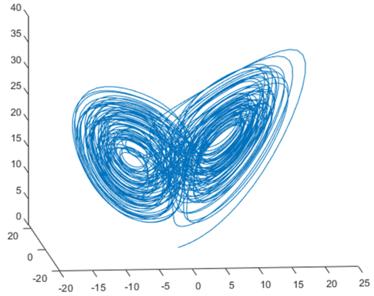
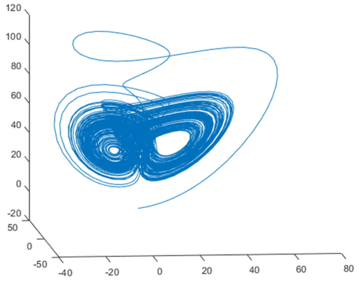
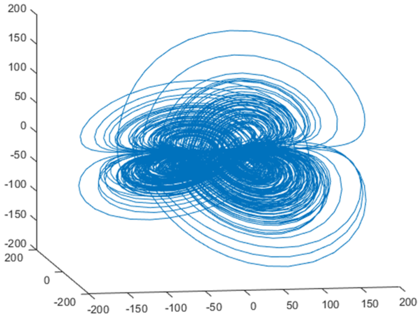
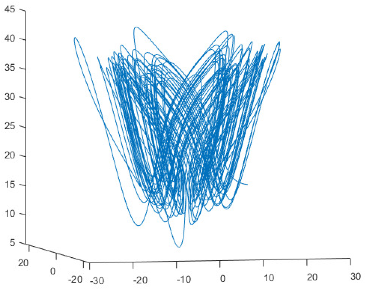
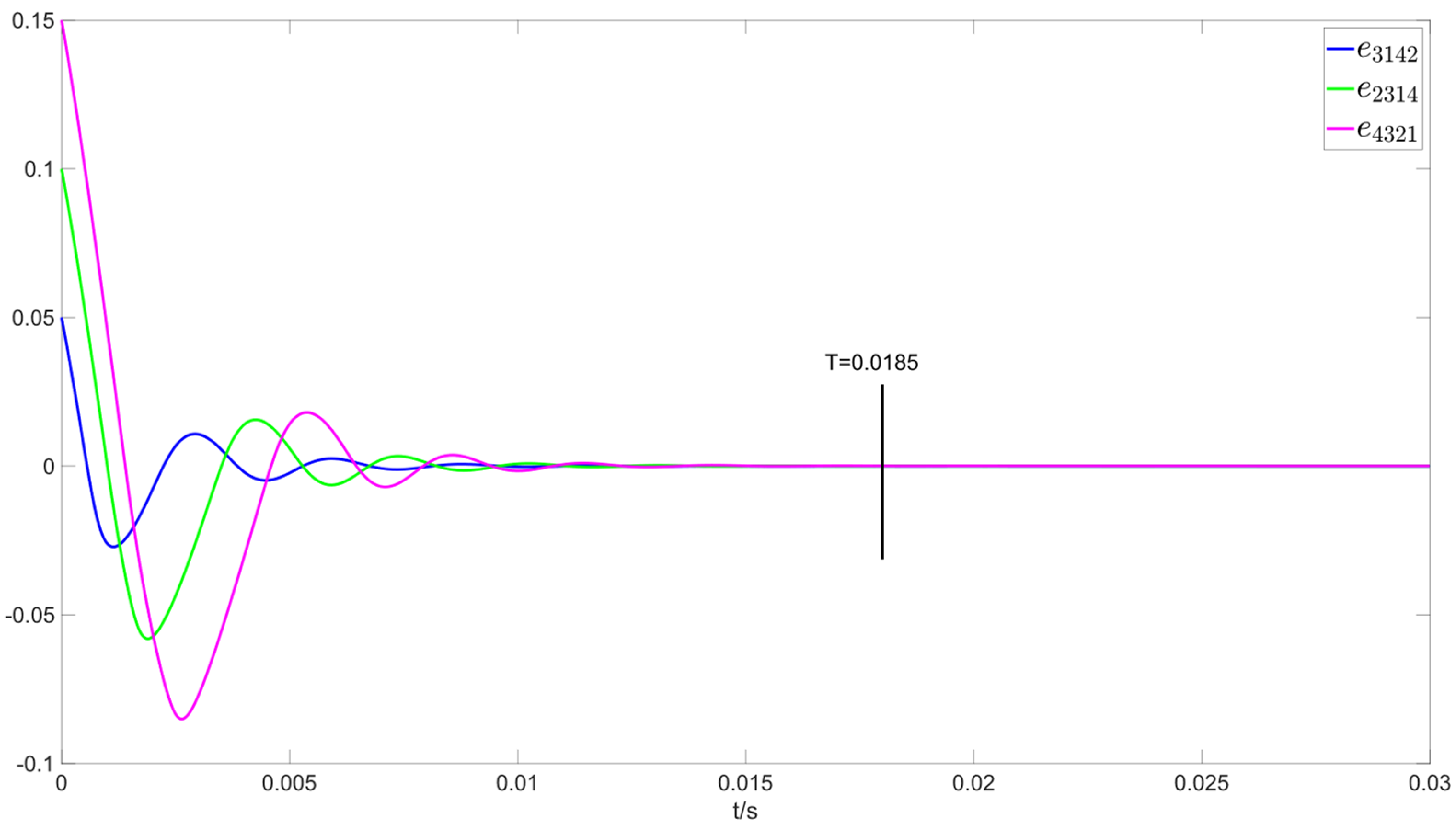
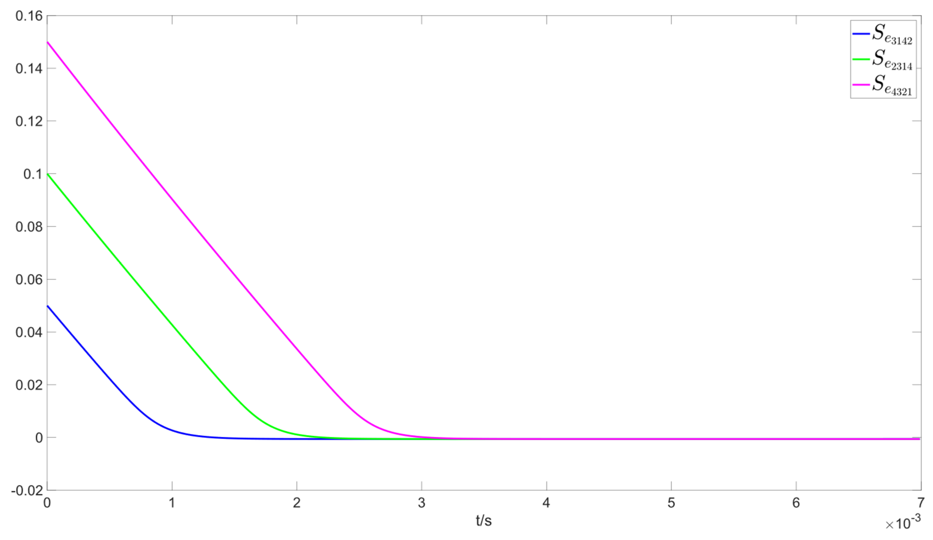
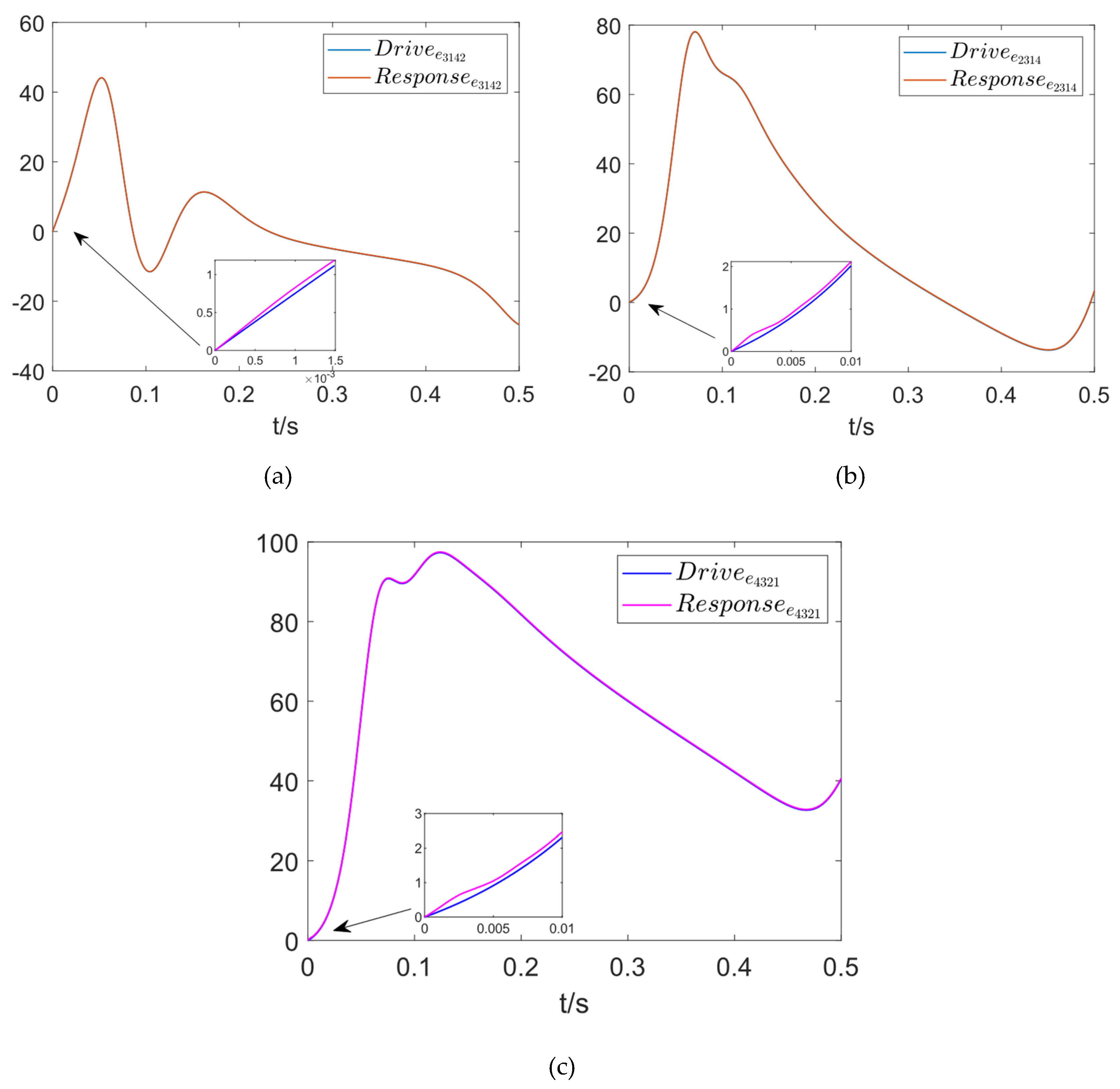
5. Numerical Simulation

In this section, the main focus is to verify the synchronization effect of the FO hyperchaotic system by means of numerical simulations and to show the validity of the Lyapunov condition proposed in this paper and whether the error system is able to reach the MSCCS within a predefined time under the action of the slide mode controller. All the numerical simulations in this paper are based on MATLAB2022a and SIMULINK2022a platforms, and the Dormand–Prince solver is chosen to solve the differential equations.

In the numerical simulation session, the drive and response systems from the previous section will be replaced with four specific FO hyperchaotic systems to facilitate subsequent validation in combination synchronization numerical simulations. The specific mathematical expression of the drive system is shown in

Table 1. The drive systems.

Drive Systems	FO Hyperchaotic Systems
Hegazi et al. [52]	$\begin{array}{l}{D}^{\mathsf{\alpha }}{x}_1\left(t\right)=a_1\left(x_2-x_1\right)+x_4+\Delta f_1(x_1,t)+d_1^f(t)\\ D^{\alpha }{x}_2\left(t\right)=a_2{x}_1-x_1{x}_3+a_3{x}_2+\Delta f_2(x_2,t)+d_2^f(t)\\ D^{\alpha }{x}_3\left(t\right)={x_{1}x}_2-a_4{x}_3+\Delta f_3(x_3,t)+d_3^f(t)\\ D^{\alpha }{x}_4\left(t\right)=x_2{x}_3+a_5{x}_4+\Delta f_4(x_4,t)+d_4^f(t)\end{array}$	(22)
Gao et al. [53]	$\begin{array}{l}{D}^{\mathsf{\alpha }}{y}_1\left(t\right)={-b}_1{y}_1+b_2{y}_2+\Delta {\mathrm{g}}_1(y_1,t)+d_1^{\mathrm{g}}(t)\\ D^{\mathsf{\alpha }}{y}_2\left(t\right)=b_3{y}_1-y_1{y}_3-y_2+y_4+\Delta {\mathrm{g}}_2(y_2,t)+d_2^{\mathrm{g}}(t)\\ D^{\mathsf{\alpha }}{y}_3\left(t\right)=y_1^2-b_4\left(y_1+y_3\right)+\Delta {\mathrm{g}}_3(y_3,t)+d_3^{\mathrm{g}}(t)\\ D^{\mathsf{\alpha }}{y}_4\left(t\right)=-b_5{y}_1+\Delta {\mathrm{g}}_4(y_4,t)+d_4^{\mathrm{g}}(t)\end{array}$	(23)

below:

• where the system parameters are $a_1=35$, $a_2=7$, $a_3=12$, $a_4=3$, $a_5=0.3$, $b_1=25,$ $b_2=60$, $b_3=40$, $b_4=4$, $b_5=5$, and $\alpha =0.95$, and $x_i(t)$, $y_i(t) (i=\mathrm{1,2},\mathrm{3,4})$ represent the state vectors of different hyperchaotic systems. Moreover, the parameter uncertainties and the external disturbances in drive FO hyperchaotic systems are

$$\begin{array}{l}\Delta f_1\left(x_1,t\right)=0.1x_{1}sin\left(t\right),d_1^f\left(t\right)=0.1sin\left(2t\right)\\ \Delta f_2\left(x_2,t\right)=0.1x_{2}sin\left(5t\right),d_2^f\left(t\right)=0.1sin\left(t\right)\\ \Delta f_3\left(x_3,t\right)=0.1x_{3}sin\left(4t\right),d_3^f\left(t\right)=0.1sin\left(2/3t\right)\\ \Delta f_4\left(x_4,t\right)=0.1x_{4}sin\left(3t\right),d_4^f\left(t\right)=0.1sin\left(1/3t\right)\\ \Delta {\mathrm{g}}_1\left(y_1,t\right)=0.1y_{1}sin\left(2t\right),d_1^{\mathrm{g}}\left(t\right)=0.1sin\left(4/5t\right)\\ \Delta {\mathrm{g}}_2\left(y_2,t\right)=0.1y_{2}sin\left(3t\right),d_2^{\mathrm{g}}\left(t\right)=0.1sin\left(3/2t\right)\\ \Delta {\mathrm{g}}_3\left(y_3,t\right)=0.1y_{3}sin\left(4t\right),d_3^{\mathrm{g}}\left(t\right)=0.1sin\left(1/2t\right)\\ \Delta {\mathrm{g}}_4\left(y_4,t\right)=0.1y_{4}sin\left(3t\right),d_4^{\mathrm{g}}\left(t\right)=0.1sin\left(t\right)\end{array}$$

(24)

The numerical simulation phase trajectory of the drive systems is shown in Figure 1 and Figure 2.

The response systems in the numerical simulation are shown in

Table 2. The FO hyperchaotic response systems.

Response Systems	FO Hyperchaotic Systems
Nabil et al. [5]	$\begin{array}{c}{D}^{\alpha }{w}_1\left(t\right)=c_1\left(w_1(t)-w_4\right)-w_2{w}_3+\Delta h_1(w_1,t)+d_1^h(t)+u_1(t)\hfill \\ D^{\alpha }{w}_2\left(t\right)=-c_2{w}_2+w_1{(t)w}_3+\Delta h_2(w_2,t)+d_2^h(t)+u_2(t)\hfill \\ D^{\mathsf{\alpha }}{w}_3\left(t\right)=-c_3{w}_3+w_1(t)\left(w_2+w_4\right)+\Delta h_3(w_3,t)+d_3^h(t)+u_3(t)\hfill \\ D^{\alpha }{w}_4\left(t\right)=c_4{w}_2{w}_3+\Delta h_4(w_4,t)+d_4^h(t)+u_4(t)\hfill \end{array}$	(25)
Pan et al. [54]	$\begin{array}{c}{D}^{\alpha }{z}_1\left(t\right)=d_1\left(z_2-z_1\right)+z_4+\Delta r_1(z_1,t)+d_1^r(t)+u_1^{*}(t)\hfill \\ D^{\alpha }{z}_2\left(t\right)=d_3{z}_1-z_1{z}_3\left(t\right)+\Delta r_2(z_2,t)+d_2^r(t)+u_2^{*}(t)\hfill \\ D^{\alpha }{z}_3\left(t\right)=z_1{z}_2-d_2{z}_3\left(t\right)+\Delta r_3(z_3,t)+d_3^r(t)+u_3^{*}(t)\hfill \\ D^{\alpha }{z}_4\left(t\right)=-z_1{z}_3\left(t\right)+d_4{z}_4+\Delta r_4(z_4,t)+d_4^r(t)+u_4^{*}(t)\hfill \end{array}$	(26)

.

• where the system parameters are $c_1=14$, $c_2=30$, $c_3=60$, $c_4=0.1$, $d_1=10,$ $d_2=8∕3$, $d_3=28$, $d_4=1.3$, and $\alpha =0.95$, and $w_i(t)$, $z_i(t)(i=1,2,3,4)$ are the state vectors of different hyperchaotic systems, and the time. Moreover, the parameter uncertainties and the external disturbances in response to FO hyperchaotic systems are

  $$\begin{array}{l}\Delta h_1\left(w_1,t\right)=0.1w_{1}sin(5t),d_1^h(t)=0.1sin(t)\\ \Delta h_2\left(w_2,t\right)=0.1w_{2}sin(2t),d_2^h(t)=0.1sin(1/3t)\\ \Delta h_3\left(w_3,t\right)=0.1w_{3}sin(2/5t),d_3^h(t)=0.1sin(2/3t)\\ \Delta h_4\left(w_4,t\right)=0.1w_{4}sin(1/5t),d_4^h(t)=0.1sin(1/2t)\\ \Delta r_1\left(z_1,t\right)\&=0.1z_{1}sin(2t),d_1^r(t)=0.1sin(1/5t)\\ \Delta r_2\left(z_2,t\right)\&=0.1z_{2}sin(t),d_2^r(t)=0.1sin(1/2t)\\ \Delta r_3\left(z_3,t\right)\&=0.1z_{3}sin(1/4t),d_3^r(t)=0.1sin(2t)\\ \Delta r_4\left(z_4,t\right)\&=0.1z_{4}sin(1/5t),d_4^r(t)=0.1sin(t)\end{array}$$

  (27)

The numerical simulation phase trajectory of the response systems is shown in Figure 3 and Figure 4

For multi-switch combination–combination synchronization, each FO hyperchaotic subsystem in the drive and response systems has four state variables, which can be freely combined among them to form a new combination system. For the drive and response systems in this paper, the main components of the multi-switch combination–combination system are schematically shown in the following Figure 5, and there are mainly 256 combinations that can be selected.

One of the combinations will be described in detail in the following section, which is used to verify the control effect of the proposed slide mode controller and slide mode surface.

$$\begin{array}{l}{e}_{3142}={\alpha }_3{x}_3+{\beta }_1{y}_1-{\gamma }_4{w}_4-{\delta }_2{z}_2\\ e_{2314}={\alpha }_2{x}_2+{\beta }_3{y}_3-{\gamma }_1{w}_1-{\delta }_4{z}_4\\ e_{4321}={\alpha }_4{x}_4+{\beta }_3{y}_3-{\gamma }_2{w}_2-{\delta }_1{z}_1\end{array}$$

(28)

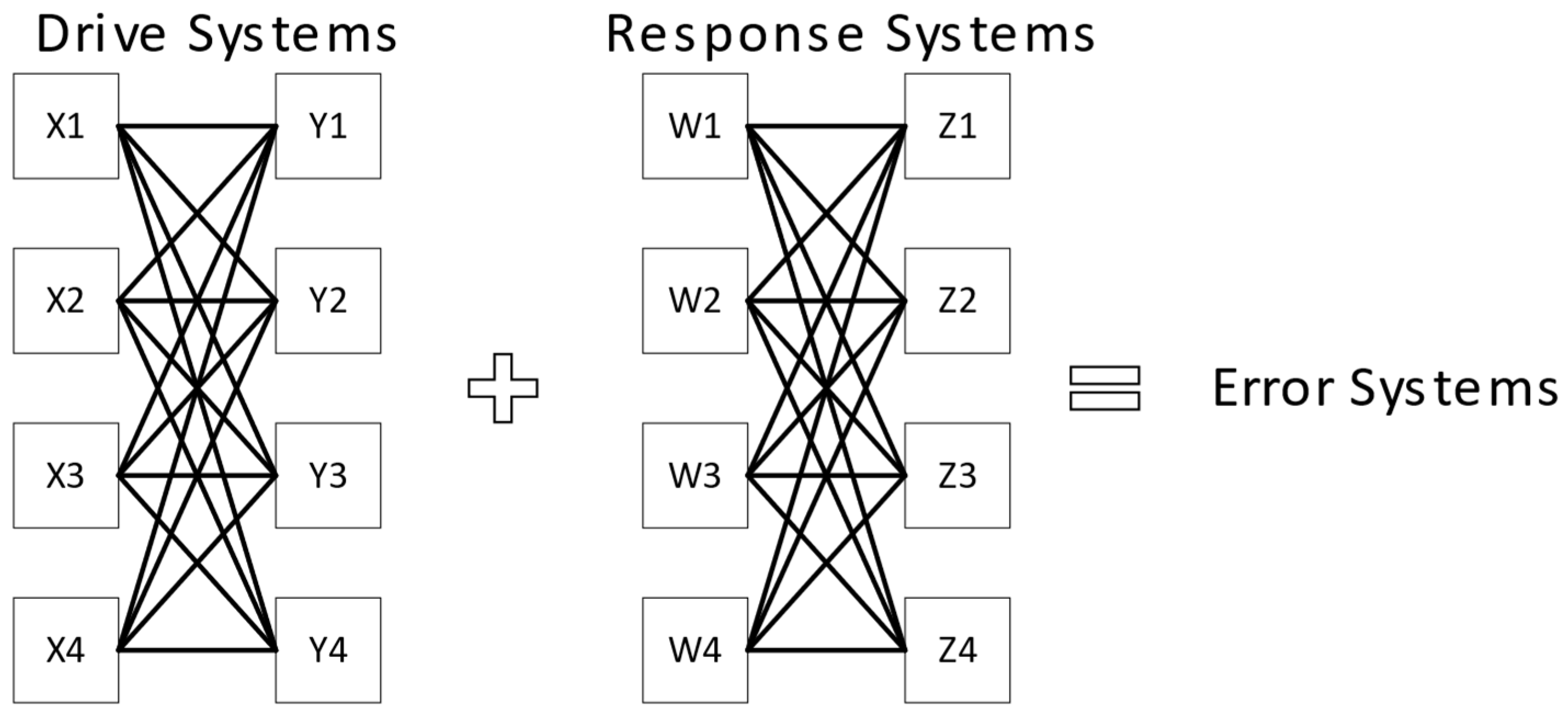
Predefined Time Multi-Switch Combination–Combination Synchronization

First define the scale matrix P as $N=P=R=Q=diag\left(\mathrm{1,1},\mathrm{1,1}\right)$, $k_i=k_i^{\Delta f}+k_i^{df}+k_i^{\Delta g}+k_i^{dg}+k_i^{\Delta h}+k_i^{dh}+k_i^{\Delta r}+k_i^{dr}=3 (i=\mathrm{1,2},\mathrm{3,4})$, the parameter $n=12$, $\alpha =0.95$, and $T_{c_1}=T_{c_2}=0.2$. Therefore, ${\phi }_1={\phi }_3=15\pi , {\phi }_2={\phi }_4={\displaystyle \frac{\pi }{0.8}}$.

According to error systems (28), the FO error systems can be expressed as

$$\begin{array}{l}{D^{\alpha }e}_{3142}={D^{\alpha }x}_3+{D^{\alpha }y}_1-D^{\alpha }{w}_4-{D^{\alpha }z}_2\\ {D^{\alpha }e}_{2314}={D^{\alpha }x}_2+D^{\alpha }{y}_3-{D^{\alpha }w}_1-{D^{\alpha }z}_4\\ {D^{\alpha }e}_{4321}={D^{\alpha }x}_4+{D^{\alpha }y}_3-D^{\alpha }{w}_2-D^{\alpha }{z}_1\end{array}$$

(29)

By considering the specific functional forms of each system, we can obtain:

$$\begin{array}{cc}\hfill D^{\mathsf{\alpha }}{e}_{3142}=x_1{x}_2& -3x_3+0.1x_{3}sin\left(4t\right)+0.1sin\left(2/3t\right)-25y_1+60y_2\hfill \\ & +0.1y_{1}sin\left(2t\right)+0.1sin\left(4/5t\right)-0.1w_2{w}_3\hfill \\ & -0.1w_{4}sin\left(1/5t\right)-0.1sin\left(1/2t\right)-28z_1+z_1{z}_3\left(t-{\mathsf{\tau }}_4\right)\hfill \\ & -0.1z_{2}sin\left(t\right)-0.1sin\left(1/2t\right)-U_{3142}(x,y,w,z)\hfill \\ \hfill D^{\mathsf{\alpha }}{e}_{2314}=7x_1& -x_1{x}_3+12x_2+0.1x_{2}sin\left(5t\right)+0.1sin\left(t\right)+y_1^2-4\left(y_1+y_3\right)\hfill \\ & +0.1y_{3}sin\left(4t\right)+0.1sin\left(1/2t\right)-14\left(w_1-w_4\right)+w_2{w}_3\hfill \\ & -0.1w_{1}sin\left(5t\right)-0.1sin\left(t\right)+z_1{z}_3-1.3z_4-0.1z_{4}sin\left(1/5t\right)\hfill \\ & -0.1sin\left(t\right)-U_{2314}(x,y,w,z)\hfill \\ \hfill D^{\mathsf{\alpha }}{e}_{4321}=x_2{x}_3& +0.3x_4+0.1x_{4}sin\left(3t\right)+0.1sin\left(1/3t\right)+{y_1}^2-4\left(y_1+y_3\right)\hfill \\ & +0.1y_{3}sin\left(4t\right)+0.1sin\left(1/2t\right)+30w_2-w_1{w}_3\hfill \\ & -0.1w_{2}sin\left(2t\right)-0.1sin\left(1/3t\right)-10\left(z_2-z_1\right)-z_4\hfill \\ & -0.1z_{1}sin\left(2t\right)-0.1sin\left(1/5t\right)\hfill \end{array}$$

(30)

For the error systems in the above Equation (30), the corresponding controller is shown below:

$$\begin{array}{cc}\hfill U_{3142}\left(x,y,w,z\right)& =x_1{x}_2-3x_3-25y_1+60y_2-0.1w_2{w}_3-28z_1+z_1{z}_3\hfill \\ & +I\left(D^{\alpha }\left({\phi }_{1}sign\left(e\right)exp(e·sign(e))+{\phi }_{2}sign\left(e\right)exp\left(-e·sign(e)\right)\right)\right)\hfill \\ & +{\phi }_{3}sign\left(s\right)exp(s·sign(s))+{\phi }_{4}sign\left(s\right)exp(-s·sign(s))+N{k}_3^{\Delta f}\hfill \\ & +N{k}_3^{df}+P{k}_1^{\Delta g}+P{k}_1^{dg}+R{k}_4^{\Delta h}+R{k}_4^{dh}+Q{k}_2^{\Delta r}+Q{k}_2^{dr}\hfill \\ \hfill U_{2314}\left(x,y,w,z\right)& =3x_1-x_1{x}_3+12x_2+y_1^2-4\left(y_1+y_3\right)-14\left(w_1-w_4\right)+w_2{w}_3+z_1{z}_3\hfill \\ & -1.3z_4\hfill \\ & +I\left(D^{\alpha }\left({\phi }_{1}sign\left(e\right)exp(e·sign(e))+{\phi }_{2}sign\left(e\right)exp\left(-e·sign(e)\right)\right)\right)\hfill \\ & +{\phi }_{3}sign\left(s\right)exp(s·sign(s))+{\phi }_{4}sign\left(s\right)exp(-s·sign(s))+N{k}_2^{\Delta f}\hfill \\ & +N{k}_2^{df}+P{k}_3^{\Delta g}+P{k}_3^{dg}+R{k}_1^{\Delta h}+R{k}_1^{dh}+Q{k}_4^{\Delta r}+Q{k}_4^{dr}\hfill \\ \hfill U_{4321}(x,y,w,z)& =x_2{x}_3+0.3x_4{{+y}_1}^2-4\left(y_1+y_3\right)+30w_2-w_1{w}_3-10\left(z_2-z_1\right)-z_4\hfill \\ & +I\left(D^{\alpha }\left({\phi }_{1}sign\left(e\right)exp(e·sign(e))+{\phi }_{2}sign\left(e\right)exp\left(-e·sign(e)\right)\right)\right)\hfill \\ & +{\phi }_{3}sign\left(s\right)exp(s·sign(s))+{\phi }_{4}sign\left(s\right)exp(-s·sign(s))+N{k}_4^{\Delta f}\hfill \\ & +N{k}_4^{df}+P{k}_3^{\Delta g}+P{k}_3^{dg}+R{k}_2^{\Delta h}+R{k}_2^{dh}+Q{k}_1^{\Delta r}+Q{k}_1^{dr}\hfill \end{array}$$

(31)

Then, according to Equation (12), the sliding mode surfaces are expressed as:

$$\begin{array}{cc}\hfill s_{3142}=I\left(D^{\alpha }{e}_{3142}\right)& \\ & +I^2(D^{\alpha }({\phi }_{1}sign\left(e_{3142}\right)exp(e_{3142}·sign({\phi }_1{e}_{3142}))\hfill \\ & +{\phi }_{2}sign\left(e_{3142}\right)exp-e_{23142}·sign(e_{3142}))))\hfill \\ \hfill s_{2314}=I\left(D^{\alpha }{e}_{2314}\right)& \\ & +I^2(D^{\alpha }({\phi }_{1}sign\left(e_{2314}\right)exp(e_{2314}·sign({\phi }_1{e}_{2314}))\hfill \\ & +{\phi }_{2}sign\left(e_{2314}\right)exp(-e_{2314}·sign(e_{2314}))))\hfill \\ \hfill s_{4321}=I\left(D^{\alpha }{e}_{4321}\right)& \\ & +I^2(D^{\alpha }({\phi }_{1}sign\left(e_{4321}\right)exp(e_{4321}·sign({\phi }_1{e}_{4321}))\hfill \\ & +{\phi }_{2}sign\left(e_{4321}\right)exp(-e_{4321}·sign(e_{4321}))))\hfill \end{array}$$

(32)

Therefore, the subsequent numerical simulation process can be carried out based on the error system, the controller, and the sliding mode surface defined above.

Remark 7.

To be able to weaken the chattering due to the sign function in the sliding mode control, the $sign\left(·\right)$ function will be replaced by the $tanh\left(100·\right)$ in all numerical simulations, and the effectiveness of the method has been demonstrated through experiments.

It can be obtained from Figure 6 that the synchronization time of the FO hyperchaotic system with three different combinations is $0.0185s$. Figure 7 shows the trajectories of the different sliding mode surfaces. The effect of synchronization of the response system in the three combination systems with the drive system under the action of the slide mode controller is shown in Figure 8.

It can be obtained from the results that the drive and response systems are still able to reach an error of zero within a certain time under the special system combination approach, which is also known as reaching system synchronization. In addition, the synchronization time of the system is $0.0185s<T_c$, which is as expected in the design of the system, and it is able to achieve predefined time synchronization. Not only that, considering the system’s anti-interference, the system is still able to achieve better synchronization with the addition of system parameter uncertainties and external disturbances, so the system has strong robustness.

When the system is designed, different values of parameter $n$ will also affect the synchronization effect of the whole FO hyperchaotic system. Therefore, one of the combined error systems $e_{4321}$ is selected as an example, and the values of the parameter $n$ are chosen as 2, 8, 12, 20, and 30, respectively, and the simulation results of the error system $e_{4321}$ are shown in Figure 9.

For hyperchaotic systems, their unique uncertain, irreducible, and unpredictable dynamics are well suited for applications in cryptography with unique advantages. Not only that, the multi-switch combination synchronization of combination systems proposed in this paper is capable of combining 256 rich combinations. This provides various flexible choices for various encryption means and also reduces the probability of encryption being broken.

6. Results

In this paper, a new Lyapunov stabilization criterion and a predefined time stabilization theory are proposed so that the FO hyperchaotic drive and response systems can be quickly synchronized under fractional-order sliding mode control. Firstly, for the predefined time stabilization theory, this paper designs a new predefined time sliding mode control strategy, which enables the system to be stabilized in a predefined time without depending on the initial conditions of the systems. Secondly, the problem of predefined time multi-switch combination–combination synchronization in FO hyperchaotic systems is explored, and based on the new predefined time sliding mode control strategy, suitable FO sliding mode controllers and sliding mode surfaces are designed so that the system can achieve predefined time synchronization in this special combination case. Not only that, the system can achieve the original intention of the system design even though parameter uncertainties and external disturbances are taken into account. Finally, the effectiveness of the proposed system is verified by numerical simulation experiments of any set of FO hyperchaotic systems, and the synchronization time of the system is much lower than the set synchronization time.

References

1. Ye, K.; Zhao, J.; Zhang, Y.; Liu, X.; Zhang, H. A Generalized Computationally Efficient Copula-Polynomial Chaos Framework for Probabilistic Power Flow Considering Nonlinear Correlations of PV Injections. Int. J. Electr. Power Energy Syst. 2022, 136, 107727. [Google Scholar] [CrossRef]
2. Veeresha, P. The Efficient Fractional Order Based Approach to Analyze Chemical Reaction Associated with Pattern Formation. Chaos Solitons Fractals 2022, 165, 112862. [Google Scholar] [CrossRef]
3. Liu, D.; Gao, X.; An, H.; Jia, N.; Wang, A. Exploring Market Instability of Global Lithium Resources Based on Chaotic Dynamics Analysis. Resour. Policy 2024, 88, 104373. [Google Scholar] [CrossRef]
4. Gong, L.; Qiu, K.; Deng, C.; Zhou, N. An Image Compression and Encryption Algorithm Based on Chaotic System and Compressive Sensing. Opt. Laser Technol. 2019, 115, 257–267. [Google Scholar] [CrossRef]
5. Nabil, H.; Tayeb, H. A Secure Communication Scheme Based on Generalized Modified Projective Synchronization of a New 4-D Fractional-Order Hyperchaotic System. Phys. Scr. 2024, 99, 095203. [Google Scholar] [CrossRef]
6. Shi, Q.; An, X.; Xiong, L.; Yang, F.; Zhang, L. Dynamic Analysis of a Fractional-Order Hyperchaotic System and Its Application in Image Encryption. Phys. Scr. 2022, 97, 045201. [Google Scholar] [CrossRef]
7. Alsaadi, F.E.; Jahanshahi, H.; Yao, Q.; Mou, J. Recurrent Neural Network-Based Technique for Synchronization of Fractional-Order Systems Subject to Control Input Limitations and Faults. Chaos Solitons Fractals 2023, 173, 113717. [Google Scholar] [CrossRef]
8. Marwan, M.; Li, F.; Ahmad, S.; Wang, N. Mixed Obstacle Avoidance in Mobile Chaotic Robots with Directional Keypads and Its Non-Identical Generalized Synchronization. Nonlinear Dyn. 2024, 113, 2377–2390. [Google Scholar] [CrossRef]
9. Pecora, L.M.; Carroll, T.L. Synchronization in Chaotic Systems. Phys. Rev. Lett. 1990, 64, 821–824. [Google Scholar] [CrossRef]
10. Bi, Y.; Zhang, H.; Qiu, R.; Wang, T.; Qiu, J. Event-Triggered Adaptive Backstepping Dynamic Surface Control for Strict-Feedback Fractional-Order Nonlinear Systems. In Proceedings of the 2022 China Automation Congress (CAC), Xiamen, China, 25 November 2022; IEEE: Piscataway, NJ, USA, 2022; pp. 3824–3828. [Google Scholar]
11. Tavazoei, M.S. Fractional Order Chaotic Systems: History, Achievements, Applications, and Future Challenges. Eur. Phys. J. Spec. Top. 2020, 229, 887–904. [Google Scholar] [CrossRef]
12. Sheu, L.-J.; Chen, H.-K.; Chen, J.-H.; Tam, L.-M. Chaos in a New System with Fractional Order. Chaos Solitons Fractals 2007, 31, 1203–1212. [Google Scholar] [CrossRef]
13. Ren, L.; Li, S.; Banerjee, S.; Mou, J. A New Fractional-Order Complex Chaotic System with Extreme Multistability and Its Implementation. Phys. Scr. 2023, 98, 055201. [Google Scholar] [CrossRef]
14. Yousefpour, A.; Jahanshahi, H.; Munoz-Pacheco, J.M.; Bekiros, S.; Wei, Z. A Fractional-Order Hyper-Chaotic Economic System with Transient Chaos. Chaos Solitons Fractals 2020, 130, 109400. [Google Scholar] [CrossRef]
15. Korneev, I.A.; Semenov, V.V.; Slepnev, A.V.; Vadivasova, T.E. Complete Synchronization of Chaos in Systems with Nonlinear Inertial Coupling. Chaos Solitons Fractals 2021, 142, 110459. [Google Scholar] [CrossRef]
16. Khan, A.; Nigar, U. Combination Projective Synchronization in Fractional-Order Chaotic System with Disturbance and Uncertainty. Int. J. Appl. Comput. Math. 2020, 6, 97. [Google Scholar] [CrossRef]
17. Wu, X.; Lu, Y. Generalized Projective Synchronization of the Fractional-Order Chen Hyperchaotic System. Nonlinear Dyn. 2009, 57, 25–35. [Google Scholar] [CrossRef]
18. Das, S.; Srivastava, M.; Leung, A.Y.T. Hybrid Phase Synchronization between Identical and Nonidentical Three-Dimensional Chaotic Systems Using the Active Control Method. Nonlinear Dyn. 2013, 73, 2261–2272. [Google Scholar] [CrossRef]
19. Zheng, S. Multi-Switching Combination Synchronization of Three Different Chaotic Systems via Nonlinear Control. Optik 2016, 127, 10247–10258. [Google Scholar] [CrossRef]
20. Hailong, Z.; Ding, Z.; Wang, L. Predefined-Time Multi-Switch Combination-Combination Synchronization of Fractional-Order Chaotic Systems with Time Delays. Phys. Scr. 2024, 99, 105223. [Google Scholar] [CrossRef]
21. Pan, W.; Li, T.; Wang, Y. The Multi-Switching Sliding Mode Combination Synchronization of Fractional Order Non-Identical Chaotic System with Stochastic Disturbances and Unknown Parameters. Fractal Fract. 2022, 6, 102. [Google Scholar] [CrossRef]
22. Vincent, U.E.; Saseyi, A.O.; McClintock, P.V.E. Multi-Switching Combination Synchronization of Chaotic Systems. Nonlinear Dyn 2015, 80, 845–854. [Google Scholar] [CrossRef]
23. Jang, S.G.; Yoo, S.J. Predefined-time-synchronized Backstepping Control of Strict-feedback Nonlinear Systems. Int. J. Robust Nonlinear Control 2023, 33, 7563–7582. [Google Scholar] [CrossRef]
24. Yan, W.; Jiang, Z.; Huang, X.; Ding, Q. Adaptive Neural Network Synchronization Control for Uncertain Fractional-Order Time-Delay Chaotic Systems. Fractal Fract. 2023, 7, 288. [Google Scholar] [CrossRef]
25. Hao, Y.; Fang, Z.; Liu, H. Adaptive T-S Fuzzy Synchronization for Uncertain Fractional-Order Chaotic Systems with Input Saturation and Disturbance. Inf. Sci. 2024, 666, 120423. [Google Scholar] [CrossRef]
26. Su, H.; Luo, R.; Huang, M.; Fu, J. Practical Fixed Time Active Control Scheme for Synchronization of a Class of Chaotic Neural Systems with External Disturbances. Chaos Solitons Fractals 2022, 157, 111917. [Google Scholar] [CrossRef]
27. Taghvafard, H.; Erjaee, G.H. Phase and Anti-Phase Synchronization of Fractional Order Chaotic Systems via Active Control. Commun. Nonlinear Sci. Numer. Simul. 2011, 16, 4079–4088. [Google Scholar] [CrossRef]
28. Zhu, S.; Li, R.; Feng, Y.; Yan, D.; Oluwaseun Onasanya, B. Predefined-Time Sliding Mode Filtering Control of Memristor-Based Bao Hyper-Chaotic System. J. Vib. Control 2024, 1, 1–26. [Google Scholar] [CrossRef]
29. Zheng, W.; Qu, S.; Tang, Q.; Du, X. Predefined-Time Sliding Mode Control for Synchronization of Uncertain Hyperchaotic System and Application. J. Vib. Control 2024, 10775463241228649. [Google Scholar] [CrossRef]
30. Nguyen, Q.D.; Vu, D.D.; Huang, S.-C.; Giap, V.N. Fixed-Time Supper Twisting Disturbance Observer and Sliding Mode Control for a Secure Communication of Fractional-Order Chaotic Systems. J. Vib. Control 2024, 30, 2568–2581. [Google Scholar] [CrossRef]
31. Modiri, A.; Mobayen, S. Adaptive Terminal Sliding Mode Control Scheme for Synchronization of Fractional-Order Uncertain Chaotic Systems. ISA Trans. 2020, 105, 33–50. [Google Scholar] [CrossRef]
32. Zhan, Z.; Zhao, X.; Yang, R. Recurrent Neural Networks with Finite-Time Terminal Sliding Mode Control for the Fractional-Order Chaotic System with Gaussian Noise. Indian J. Phys. 2024, 98, 291–300. [Google Scholar] [CrossRef]
33. Xiong, P.-Y.; Jahanshahi, H.; Alcaraz, R.; Chu, Y.-M.; Gómez-Aguilar, J.F.; Alsaadi, F.E. Spectral Entropy Analysis and Synchronization of a Multi-Stable Fractional-Order Chaotic System Using a Novel Neural Network-Based Chattering-Free Sliding Mode Technique. Chaos Solitons Fractals 2021, 144, 110576. [Google Scholar] [CrossRef]
34. Hui, M.; Zhang, J.; Iu, H.H.-C.; Yao, R.; Bai, L. A Novel Intermittent Sliding Mode Control Approach to Finite-Time Synchronization of Complex-Valued Neural Networks. Neurocomputing 2022, 513, 181–193. [Google Scholar] [CrossRef]
35. Zhang, M.; Zang, H.; Bai, L. A New Predefined-Time Sliding Mode Control Scheme for Synchronizing Chaotic Systems. Chaos Solitons Fractals 2022, 164, 112745. [Google Scholar] [CrossRef]
36. Moreno, J.A.; Osorio, M. Strict Lyapunov Functions for the Super-Twisting Algorithm. IEEE Trans. Automat. Contr. 2012, 57, 1035–1040. [Google Scholar] [CrossRef]
37. Jing, C.; Zhang, H.; Liu, Y.; Zhang, J. Adaptive Super-Twisting Sliding Mode Control for Robot Manipulators with Input Saturation. Sensors 2024, 24, 2783. [Google Scholar] [CrossRef]
38. Wang, Y.-L.; Jahanshahi, H.; Bekiros, S.; Bezzina, F.; Chu, Y.-M.; Aly, A.A. Deep Recurrent Neural Networks with Finite-Time Terminal Sliding Mode Control for a Chaotic Fractional-Order Financial System with Market Confidence. Chaos Solitons Fractals 2021, 146, 110881. [Google Scholar] [CrossRef]
39. Wang, S. Finite-Time Synchronization of Fractional Multi-Wing Chaotic System. Phys. Scr. 2023, 98, 115224. [Google Scholar] [CrossRef]
40. Su, H.; Luo, R.; Fu, J.; Huang, M. Fixed Time Control and Synchronization of a Class of Uncertain Chaotic Systems with Disturbances via Passive Control Method. Math. Comput. Simul. 2022, 198, 474–493. [Google Scholar] [CrossRef]
41. Xiao, L.; Li, L.; Cao, P.; He, Y. A Fixed-Time Robust Controller Based on Zeroing Neural Network for Generalized Projective Synchronization of Chaotic Systems. Chaos Solitons Fractals 2023, 169, 113279. [Google Scholar] [CrossRef]
42. Assali, E.A. Predefined-Time Synchronization of Chaotic Systems with Different Dimensions and Applications. Chaos Solitons Fractals 2021, 147, 110988. [Google Scholar] [CrossRef]
43. Chen, S.; Wan, Y.; Cao, J. Predefined-Time Synchronization for FitzHugh-Nagumo Neural Networks With External Disturbances and Multiple Time Scales: An Adaptive Control Approach. In IEEE Transactions on Automation Science and Engineering; IEEE: Piscataway, NJ, USA, 2024; pp. 1–12. [Google Scholar] [CrossRef]
44. Wang, S.; Jian, J. Predefined-Time Synchronization of Fractional-Order Memristive Competitive Neural Networks with Time-Varying Delays. Chaos Solitons Fractals 2023, 174, 113790. [Google Scholar] [CrossRef]
45. Caputo, M. Linear Models of Dissipation Whose Q Is Almost Frequency Independent—II. Geophys. J. Int. 1967, 13, 529–539. [Google Scholar] [CrossRef]
46. Podlubny, I. Fractional Differential Equations; Elsevier Science and Technology: Amsterdam, The Netherlands, 1998. [Google Scholar]
47. Monje, C.A.; Chen, Y.; Vinagre, B.M.; Xue, D.; Feliu-Batlle, V. Fractional-Order Systems and Controls: Fundamentals and Applications; Springer Science & Business Media: Berlin/Heidelberg, Germany, 2010; ISBN 978-1-84996-335-0. [Google Scholar]
48. Han, J.; Chen, G.; Zhang, G.; Hu, J. Fixed/Predefined-Time Projective Synchronization for a Class of Fuzzy Inertial Discontinuous Neural Networks with Distributed Delays. Fuzzy Sets Syst. 2024, 483, 108925. [Google Scholar] [CrossRef]
49. Wang, T.; Zhao, S.; Zhou, W.; Yu, W. The Lag Projective (Anti-)Synchronization of Chaotic Systems with Bounded Nonlinearity via an Adaptive Control Scheme. Adv. Differ. Equ. 2013, 2013, 225. [Google Scholar] [CrossRef]
50. Chen, J.; Zhao, X.; Xiao, J. Novel Predefined-time Control for Fractional-order Systems and Its Application to Chaotic Synchronization. Math. Methods Appl. Sci. 2024, 47, 5427–5440. [Google Scholar] [CrossRef]
51. Luo, R.; Liu, S.; Song, Z.; Zhang, F. Fixed-Time Control of a Class of Fractional-Order Chaotic Systems via Backstepping Method. Chaos Solitons Fractals 2023, 167, 113076. [Google Scholar] [CrossRef]
52. Hegazi, A.S.; Matouk, A.E. Dynamical Behaviors and Synchronization in the Fractional Order Hyperchaotic Chen System. Appl. Math. Lett. 2011, 24, 1938–1944. [Google Scholar] [CrossRef]
53. Gao, Y.; Liang, C.; Wu, Q.; Yuan, H. A New Fractional-Order Hyperchaotic System and Its Modified Projective Synchronization. Chaos Solitons Fractals 2015, 76, 190–204. [Google Scholar] [CrossRef]
54. Pan, L.; Zhou, W.; Zhou, L.; Sun, K. Chaos Synchronization between Two Different Fractional-Order Hyperchaotic Systems. Commun. Nonlinear Sci. Numer. Simul. 2011, 16, 2628–2640. [Google Scholar] [CrossRef]
Figure 1. The system (22) in x 1 x 2 x 3 space.
Fractalfract 09 00147 g001
Figure 2. The system (23) in y 1 y 2 y 3 space.
Fractalfract 09 00147 g002
Figure 3. The system (25) in w 1 w 2 w 3 space.
Fractalfract 09 00147 g003
Figure 4. The system (26) in z 1 z 2 z 3 space.
Fractalfract 09 00147 g004
Figure 5. Multi-switch combination–combination system combination schematic.
Fractalfract 09 00147 g005
Figure 6. The evolution curves of the three error systems.
Fractalfract 09 00147 g006
Figure 7. The trajectories of the sliding mode surfaces.
Fractalfract 09 00147 g007
Figure 8. Synchronization results for three combination synchronization systems. Subfigures (ac) show the trajectory tracking curves for e 3142 , e 2314 , e 4321 respectively.
Fractalfract 09 00147 g008
Figure 9. Trajectories of the error system for different values of the parameter n.
Fractalfract 09 00147 g009