Variable-Order Time-Fractional Kelvin Peridynamics for Rock Steady Creep

Abstract

A variable-order time-fractional Kelvin peridynamics model is proposed, where the variable order is utilized to reflect the changes of viscosity in viscoelastic materials to effectively capture the damage and deformation of rock steady creep. The corresponding constitutive model is established by coupling a spring and an Abel dashpot. Through the Caputo definition of fractional-order derivatives, finite increment formulations for the constitutive model are derived to facilitate numerical implementation by an explicit time integration scheme. We accordingly introduce a model parameter evaluation method for practical applications. To verify the validity and correctness of the model, constant-order time-fractional peridynamics is used to compare with the proposed model via a sandstone compress creep numerical test, and the results show that the latter can simulate nonlinear creep behavior more efficiently. Additionally, the numerical simulation of practical engineering is conducted. Compared with constant-order time-fractional peridynamics, the proposed model can improve the simulation accuracy by 16.7% with fewer model parameters.

1. Introduction

The study of the time-dependent deformation and failure behavior of rock is essential for the long-term stability of the surrounding rock mass around underground engineering. Large deformations and time dependence are the most significant mechanical behaviors in rock rheology. Rock rheology may cause geological disasters such as collapse, water inrush, and large deformation, which seriously affect the construction safety and service life of tunnels [1]. Hence, with the development of underground engineering, the rheological properties of rock have attracted much interest for many researchers [2,3].

Creep is a specific behavior of rock rheology in tunneling engineering. Developing a precise creep model with few model parameters is significant. As illustrated in Figure 1, the creep strain curve consists of three stages: the initial decelerating creep stage, the steady-state creep stage, and the accelerating creep stage. At the primary stage, the rate initially starts high and then gradually decreases. The secondary stage is characterized by a constant rate. At the tertiary stage, the internal damage of the material increases. Consequently, the material creeps at an accelerated rate until the material fails. The whole process of creep can be viewed as the viscous, elastic, and plastic evolution process. The rock creep behavior is divided into stable creep and unsteady creep, and the occurrence of both depends on whether the constant load applied is greater than the yield strength. This paper focuses on stable creep [4,5], which is composed of the initial decelerating creep stage and steady-state creep stage. The strain rate of the rock decreases over time and eventually approaches zero, such that the rock does not enter the accelerating creep stage.

Viscoelastic materials exhibit both viscous and elastic behaviors. The classical notion of Newtonian viscosity is that the rate of strain is proportional to stress. One such material is a Kelvin material (i.e., rock and polymers), which can be represented in one dimension by a spring (with elastic constant) in parallel with a dashpot (of viscous constant). Similarly, a large number of mathematical models for viscoelastic materials with parallel or series combinations of springs and dashpots have been proposed, such as the well-known Maxwell model and Burgers model [6]. However, the above-mentioned models cannot adequately reflect the historical dependence of the deformation of viscoelastic materials. Koeller et al. [7] employed the Riemann–Liouville fractional derivative to construct a constant-order time-fractional (COTF) dashpot to replace the traditional Newton dashpot which was called Abel dashpot. The Abel dashpot has attracted widespread attention as it exhibits three major advantages: time nonlocality, flexibility in adjusting model complexity by changing the fractional order, and the ability to reduce the number of parameters while maintaining accuracy [8,9].

During the steady-state creep stage, the viscosity of the material is consumed and the ratio of viscosity to elasticity is reduced from 1 to 0, indicating that the fractional order should be assumed as a function related to time. The viscoelastic model with a variable-order time-fractional (VOTF) dashpot can be adapted to reflect the change in viscosity. During creep, the fractional order changes with time and accurately describes the viscous dissipation in the material [10]. Liu et al. [10] proposed a nonlinear damage creep model to better describe rock creep, based on the Caputo variable-order fractional derivative and continuous damage model with a sum function. In addition, for a better description of material viscosity weakening, Sun et al. [11] used the finite difference method to discretize the approximation of the variable order fractional order eigenequations and established the relationship between the fractional order and the variables based on the experimental results. Liu et al. [12] proposed a novel creep model by introducing a variable order function to consider the evolution of the damage effect. Compared to the COTF creep model, the VOTF creep model exhibits a superior ability to characterize nonlinear creep deformation, especially in the failure behavior of accelerated creep with a sharply increasing strain rate. The research demonstrated the advantages of a variable fractional order viscoelastic model.

Numerical simulation [13,14] is the main research method for studying rock creep behavior. For example, Wang et al. [15] proposed a damage-based constitutive creep model by combining the classical power law constitutive creep model with a localized damage model which was implemented in classical continuum mechanics finite element commercial software to numerically simulate the time-dependent behavior of inhomogeneous brittle rock. Classical continuum mechanics assumes that all internal forces exhibit local action [16,17]. The derived motion equations are expressed in terms of partial differential equations [18]. However, the spatial derivatives of the displacement field in the partial differential equations introduce additional complexity in representing discontinuous displacement fields when damage such as fractures or cracks is present. Hence, the numerical method based on classical continuum mechanics makes it difficult to simulate damage. Peridynamics (PD) theory, proposed by Silling [19], represents internal forces via nonlocal interactions between pairs of material points within a continuous body. Consequently, peridynamics formulations are free from the issue of spatial derivatives and provide a natural description for describing the formation and evolution of discontinuities, such as cracks and fractures due to deformations in the displacement field of elastic bodies. Peridynamics has been applied in a variety of applications, including impact damage [20], crack propagation [21], geomaterial fragmentation [22], and failure and damage in composite materials [23]. Meanwhile, peridynamics has been developed for the numerical simulation of viscoelastic materials [8,24], in which the stress–strain relations were expressed as a combination of exponentially decaying functions as an approximation to the stress–strain relations. However, an inaccurate prediction result may be obtained by the approximation methods.

We propose a variable-order time-fractional Kelvin peridynamics (VOTFK PD) model in the framework of bond-based peridynamics, where the variable order is used to reflect the change in viscosity to effectively describe the damage and the nonlinear deformation of rock stable creep. In this paper, we present the derivation of the VOTFK PD model in Section 2. The corresponding numerical discretization of the model and model parameter evaluation method is given in Section 3. Subsequently, in Section 4, we conduct numerical tests to investigate the performance of the proposed model in comparison to COTFK peridynamics and analytical results, which demonstrates the utility of the model. Finally, we conclude with remarks in Section 5.

2. Numerical Model

2.1. Kelvin Peridynamics

Bond-based peridynamics supposes that discrete material points interact with each other by a pairwise force vector. The direct physical interaction between these material points is called a bond. It has been certified that peridynamics can be used to simulate the damage process of rock material. For example, Ha et al. [25] investigated the fracturing responses of a single flaw embedded in rock-like materials under compression. Zhou et al. [26] investigated the initiation, propagation, and coalescence of cracks in brittle rock material subjected to compressive loads. Obviously, the numerical method based on peridynamics is the most simple and efficient method to simulate the deformation and damage of rock materials, and it meets the requirements of rock material calculation when the influence of Poisson’s ratio is ignored. In a homogeneous body (Figure 2), the peridynamics equation [19] of motion for any material point $x$ in the reference configuration can be given as

$$\rho \ddot{u}(x,t)={\displaystyle {\int }_{H_x}f\left(u(x^{\prime },t)-u(x,t),x^{\prime }-x\right)d{V}_{x^{\prime }}}+b(x,t)$$

(1)

where $\rho$ and $b$ are the mass density and externally applied body force density, respectively, and $u(x,t)$ is the displacement field. f represents the bond force density function and $d{V}_{x^{\prime }}$ denotes an infinitesimal volume of material point $x^{\prime }$. In the peridynamics theory, the motion of the body is analyzed by considering the interaction of a peridynamics material point $x$ with any material point $x^{\prime }$ within a horizon $H_x$ defined as $H_x=\{x^{\prime }\in R:0<‖x^{\prime }-x‖<\delta \}$.

The pairwise force function f can be expressed as a function of the relative position vector $\xi$ and the relative displacement vector $\eta$ at time t [19], which are denoted by

$$\xi =x^{\prime }-x$$

(2)

$$\eta =u(x^{\prime }, t)-u(x, t)$$

(3)

The $\xi +\eta$ represents the current relative position vector between the material points. The impact of the bond force density function f is nonlocal with a horizon δ for interaction, such that

$$\begin{array}{cc}f(\xi ,\eta )=0 & \left|\xi \right|>\delta \end{array}$$

(4)

The pairwise force function f is required to fulfill Equation (5) to ensure conservation of linear momentum and Equation (6) to ensure the conservation of angular momentum.

$$f(-\xi ,-\eta )=\mathrm{f}(\xi ,\eta ) \forall \xi , \eta$$

(5)

$$(\xi +\eta )\times f(\xi ,\eta ) \forall \xi , \eta$$

(6)

In the model, the bond force is expressed in terms of the length of the bond and direction vector, as follows:

$$\begin{array}{cc}f(\xi ,\eta )=c_{E}s{\displaystyle \frac{\xi +\eta }{‖\xi +\eta ‖}}& \left|\xi \right|\le \delta \end{array}$$

(7)

where $c_E=9E/(\pi {\delta }^{3}d)$ is the material parameter which depends on the Young’s modulus E. Then, the deformed energy of the peridynamics is consistent with the classical elastic model. The scalar function s represents the bond stretch. Silling [20] defined the bond stretch as

$$s={\displaystyle \frac{‖\xi +\eta ‖-‖\eta ‖}{\xi }}$$

(8)

Then, the motion equation of the linearized elastic peridynamics can be yielded as

$$\rho \ddot{u}(x,t)={\displaystyle {\int }_{H_x}{c}_{E}s\frac{\xi +\eta }{‖\xi +\eta ‖}d{V}_{x^{\prime }}+b(x,t)}$$

(9)

which is imposed in the domain over the time period (0, T]. The nonlocal boundary condition

$$\begin{array}{cc}u(x,t)=g(x,t)& (x,t)\in \overline{\Omega }\times \end{array}[0,T]$$

(10)

is imposed on the volume constrained boundary zone Ω_c that surrounds the domain Ω with the width δ, where g is the prescribed displacement field imposed on the Ω_c. Finally, the initial conditions are the specified initial displacement and velocity.

$$\begin{array}{cc}u(x,0)=u_0(x)& {\partial }_{t}u(x,0)={\dot{u}}_0(x) x\in \Omega \end{array}$$

(11)

Viscoelastic materials exhibit both restorative elastic solid behavior and internally dissipative Newtonian fluid behavior. To model the mechanical property, the pairwise bond force density function $f(\xi ,{\partial }_t\eta ,\eta )$ also depends on the time derivative of the relative displacement vector, ${\partial }_t\eta$, to account for the time-dependent viscous behavior of the materials. The Kelvin model (Figure 3) was chosen to describe the viscoelastic behavior of rock, which is the same as the research conducted by Mainardi, F. [27].

In classical mechanics of a continuous medium, the constitutive model of the one-dimensional Kelvin model [28] is shown in Equation (12).

$$\sigma =E\epsilon +\mu {\displaystyle \frac{\partial \epsilon }{\partial t}}$$

(12)

where $\mu$ represents the damping coefficient of the materials. In the model, the dashpot is in parallel with the spring; therefore, the spring must follow the slow deformation of the dashpot, which can better simulate the anelasticity of the rock.

Then, the constitutive equation of Kelvin peridynamics is rewritten to the following form:

$$\begin{array}{cc}f(\xi ,{\partial }_t\eta ,\eta )=c_{E}s{\displaystyle \frac{\xi +\eta }{‖\xi +\eta ‖}}+c_{\mu }\dot{s}{\displaystyle \frac{\xi +\eta }{‖\xi +\eta ‖}}& ‖\xi ‖\le \delta \end{array}$$

(13)

where $c_{\mu }=9\mu /(\pi {\delta }^{3}d)$ is determined by viscosity material parameters.

The bond stretch is used to define the failure criterion in peridynamics. When the bond stretch exceeds a predefined limit, the bond breaks. After bond failure, there is no force between two material points. Once a bond fails, it cannot heal, making the model history-dependent. The $\psi (x,\xi ,t)$ is defined as a history-dependent scalar-valued function mapping the breakage of the bond, which is expressed as

$$\psi (x,\xi ,t)=\left\{\begin{array}{c}1,s(t^{\prime },\xi )<s_0,0<t^{\prime }<t\\ 0,else\end{array}\right.$$

(14)

where $s_0$ denotes the critical stretch or failure of the bond [29], which is expressed by

$$s_0=\left\{\begin{array}{cc}\sqrt{{\displaystyle \frac{\pi G_0}{3k\delta }}}& 2D\\ \sqrt{{\displaystyle \frac{5G_0}{9k\delta }}}& 3D\end{array}\right.$$

(15)

where $G_0$ is the energy release rate [20] and k is the bulk modulus. The bond is active when $\psi =1$ and it is broken when $\psi =0$.

Damage in the materials is expressed locally by the ratio of the number of broken bonds to the number of total bonds in the field as

$$D(x,t)=1-{\displaystyle \frac{{{\displaystyle \int }}_{H_x}\psi (x,\xi ,t)d{V}_{x^{\prime }}}{{{\displaystyle \int }}_{H_x}d{V}_{x^{\prime }}}}$$

(16)

where $D(x,t)$ is a function of position and time. Note that $0\le D\le 1$, with $0$ representing the original state with no damage and $1$ representing the complete disconnection of a material point from all other points within its horizon [20].

2.2. Constant-Order Time-Fractional Kelvin Peridynamics

Fractional order derivatives can represent temporal non-locality and long-term memory characteristics in the constitutive relationship of materials, which is a significant advantage over traditional integer order models. The constitutive relationship of an Abel dashpot is

$$\sigma (t)=\mu {\displaystyle \frac{{\partial }^{\alpha }\epsilon (t)}{\partial t^{\alpha }}}$$

(17)

where α is the fractional order. The creep curves with different α are illustrated in Figure 4. Under constant stress, for 0 < α < 1, the strain increases slowly and its rate gradually decreases with time. It neither increases linearly, as do Newtonian fluids, nor remains constant, as do linear elastic bodies. The α can depict the nonlinear strain of materials between fluid and solid states. As α approaches 1, the material shows more elasticity; as α approaches 0, it exhibits more viscosity.

Viscous materials have a linear stress–strain rate relationship, which is inadequate for describing the nonlinear creep of rocks. In contrast, the constitutive relationship of the Abel dashpot features a nonlinear stress–strain or strain–rate relationship. The Caputo fractional order derivative of the function f [30] is introduced:

$$D_t^{\alpha }f(t)={\displaystyle \frac{1}{\mathsf{\Gamma }(1-\alpha )}}{\displaystyle {\int }_0^t\frac{\mathrm{d}f(\tau )}{\mathrm{d}\tau }{(t-\tau )}^{-\alpha }\mathrm{d}\tau }$$

(18)

where $\Gamma \left(x\right)$ is the Gamma function.

$$\mathsf{\Gamma }(x)={\displaystyle {\int }_0^{\infty }{\mathrm{e}}^{-t}{t}^{x-1}\mathrm{d}t}$$

(19)

Then, the stress–strain equation can be rewritten as

$$\begin{array}{c}f(t)=c_E\epsilon +c_{\mu }{\displaystyle {\int }_0^t\frac{\dot{s}(\tau )d\tau }{\Gamma (1-\alpha ){(t-\tau )}^{\alpha }}=c_E\epsilon +c_{\mu }{\partial }_t^{\alpha }\epsilon 0<\alpha <1}\end{array}$$

(20)

to accurately describe the power law behavior of viscoelastic materials [31,32]. Furthermore, fractional models can accurately capture the power law behavior of stress [33,34,35].

Then, the motion equation of constant-order time-fractional Kelvin peridynamics (COTFK PD) is Equation (21), in which the pairwise bond force density function f takes the following form:

$$\begin{array}{c}\rho \ddot{u}(x,t)={\displaystyle {\int }_{H_x}(c_{E}s\frac{\xi +\eta }{‖\xi +\eta ‖}+c_{\mu }\frac{{\partial }^{\alpha }s}{\partial t^{\alpha }}\frac{\xi +\eta }{‖\xi +\eta ‖})dV{x}^{\prime }+b(x,t) 0<\alpha <1}\end{array}$$

(21)

Obviously, the deformation increases with an increase in the fractional order [10]. The nonlinear creep behavior can be well exhibited under various orders. Different orders represent different proportions of viscosity and elasticity and also demonstrate the evolution of viscoelasticity.

2.3. Variable-Order Time-Fractional Kelvin Peridynamics

The model mentioned above in Section 2.2 cannot well characterize the time-dependence within creep behavior. It is necessary to propose a varying-order function related to time. The COTFK model can be extended to one case, in which α is assumed as a function of t. The Caputo fractional derivation for the differential operator of α(t) was introduced as follows:

$$D^{\alpha (t)}f(x)={\displaystyle \frac{1}{\Gamma (1-\alpha (t))}}{\displaystyle {\int }_a^t\frac{d}{dt}\frac{f(\tau )}{{(t-\tau )}^{\alpha (t)}}d\tau }$$

(22)

Then, the viscoelastic pairwise force can be rewritten as follows:

$$f(t)=c_{E}s(t)+c_{\mu }{\displaystyle \frac{d^{\alpha (t)}s(t)}{d{t}^{\alpha (t)}}}$$

(23)

where α(t) is the variable order function related to time. Then, the model can represent the change of viscosity during creep. In this study, the variable order function is assumed as

$$\alpha (t)=e^{-ct}$$

(24)

The order function is expressed in an exponential form because it effectively represents the rapid consumption of the viscosity of the materials [10]. Then, the viscoelastic pairwise force can be rewritten finally as follows:

$$f(t)=c_{E}s(t)+c_{\mu }{\displaystyle \frac{d^{e^{-ct}}s(t)}{d{t}^{e^{-ct}}}}$$

(25)

3. Numerical Implementation

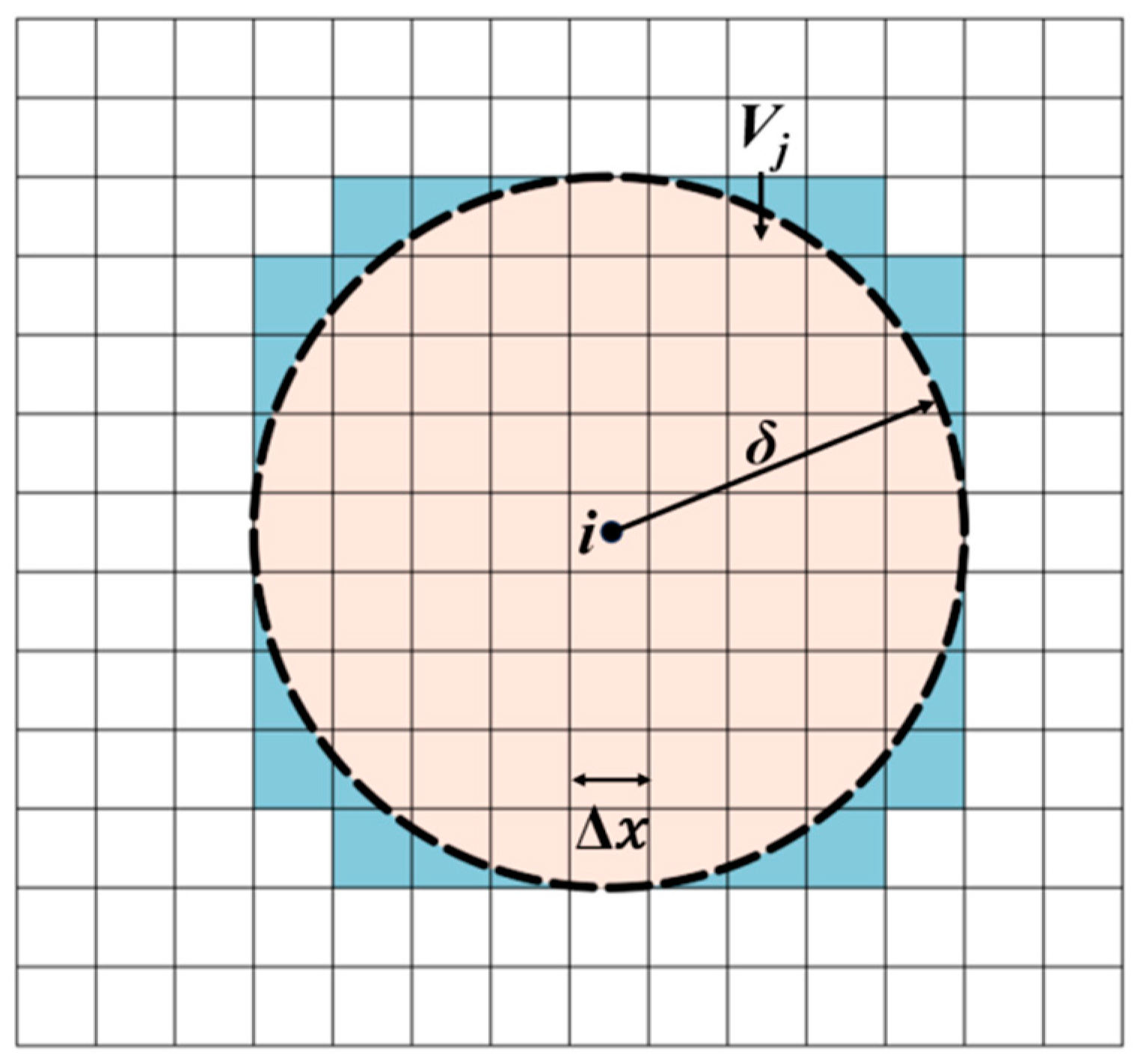
3.1. Numerical Discretization

The solution of formulation requires spatial integration, which utilizes a one-point Gaussian integration (meshless) scheme. The region of interest is uniformly discretized into material points in all analyses, each with a known volume in the reference configuration. In order to avoid numerical instability caused by the introduction of fractional derivatives, this study investigates an explicit quasi-static method, which is implemented by introducing artificial viscous damping to obtain the steady-state solution of the system. The dynamic relaxation method is to construct and solve a virtual dynamical system with damping to obtain a static solution [36]. The Rayleigh method can be used to determine the fundamental frequency and to determine the artificial damping coefficient c_n, where n is the nth time step number. There are some limitations of the explicit anamorphic method, such as the empirical dependence of the determination of the artificial damping coefficients. Therefore, the steady-state solution of Equation (26) is achieved by employing the adaptive dynamic relaxation method introduced in Ref. [37], in which the damping coefficient is changed adaptively in each time step. The motion equation is expressed as

$$c_n\ddot{u}(x,t)+c_n\dot{u}(x,t)={\displaystyle {\int }_{H_x}fdV{x}^{\prime }+b(x,t)}$$

(26)

When solving the peridynamics equations using the meshless particle method, the system is often discretized into a centrally orthogonal array of uniform particle points, the near-field range size is taken as a constant, and the spatial integration is done by a single Gaussian point integration method. The peridynamics equation of motion is an integral-differential equation, which is not usually amenable to analytical solutions. Therefore, its solution is constructed by using numerical techniques for spatial and time integrations [38]. After discretization, the integral of motion equation of the VOTF peridynamics can be replaced by a finite sum, which is

$$c_n{\ddot{u}}_i^n+c_n\dot{u}(x,t)={\displaystyle {\sum }_{j}f({\xi }^n,{\eta }^n)}{V}_j+b_i^n$$

(27)

$$f({\xi }^n,{\eta }^n)={\displaystyle \sum _j(c_E{s}^n\frac{\xi +{\eta }^n}{\left|\xi +{\eta }^n\right|}+c_{\mu }\frac{{\partial }^{\alpha (t)}{s}^n}{\partial t^{\alpha (t)}}\frac{\xi +{\eta }^n}{\left|\xi +{\eta }^n\right|})d{V}_j}$$

(28)

where i and j denote the node numbers, and V_j is the volume of the node j. Using the explicit integration method of center difference, the velocity and displacement of the next time step can be obtained as

$${\dot{U}}^{n+1/2}={\displaystyle \frac{(2-c^n\Delta t){\dot{U}}^{n-1/2}+2\Delta t{D}^{-1}{F}^n}{(2+c^n\Delta t)}}$$

(29)

$$U^{n+1}=U^n+\Delta t{\dot{U}}^{n+1/2}$$

(30)

The above equation can not be used at the beginning of the iteration, but it can still be assumed that $U^0=0$ and ${\dot{U}}^0=0$. Then, the iteration calculation begins with

$${\dot{U}}^{1/2}={\displaystyle \frac{2\Delta t{D}^{-1}{F}^0}{2}}$$

(31)

The calculation process of the virtual diagonal density matrix D and nth damping coefficient c_n can be determined by referring to the study of Underwood et al. [37].

The L1 temporal discretization scheme is employed to approximate the fractional-order derivative. Specifically, the time interval $[0,T]$ is partitioned into $N$ uniform subintervals with time steps $t_n=n\Delta t(n=0,1,\dots ,N)$, where $\Delta t=T/N$ denotes the temporal step size. The discrete approximations of field variables are defined at each temporal node as $f_n:=f(x,t_n)$, $c_n:=c(x,t_n)$, and $s_n:=s(x,t_n)$. We discretize ${\partial }_{t}s$ and ${\partial }_t^{\alpha (t)}s$ by

$${\partial }_{t}s(x,t_n)={\delta }_{\tau }{s}_n+E_n:={\displaystyle \frac{s_n-s_{n-1}}{\tau }}+{\displaystyle \frac{1}{\tau }}{\displaystyle {\int }_{t_{n-1}}^{t_n}{\partial }_t^{2}s(x,t)(t-t_{n-1})dt,}$$

(32)

$${\partial }_t^{\alpha (t_n)}s(x,t_n)=\sum _{k=1}^n{\displaystyle {\int }_{t_{k-1}}^{t_k}\frac{{\partial }_{s}u(x,z)dz}{\mathsf{\Gamma }(1-\alpha (z)){(t_n-z)}^{\alpha (z)}}}={\delta }_{\tau }^{\alpha (t_n)}{s}_n$$

(33)

for $1\le n\le N$. Here, ${\delta }_{\tau }^{\alpha (t_n)}{s}_n$ is defined by

$${\delta }_{\tau }^{\alpha (t_n)}{s}_n:=\sum _{k=1}^n{b}_{n,k}(u_k-u_{k-1})=b_{n,n}{s}_n+\sum _{k=1}^{n-1}(b_{n,k}-b_{n,k+1})s_k,$$

(34)

$$b_{n,k}:={\displaystyle \frac{{\left(t_n-t_{k-1}\right)}^{1-\alpha (t_k-1)}-{\left(t_n-t_k\right)}^{1-\alpha (t_k-1)}}{\Gamma \left(2-\alpha \left(t_k-1\right)\right)\tau }}$$

(35)

The material points x_i are acted by other material points x_j ($‖x_j-x_i‖\le \delta$) in the near-field range. However, some material points are only partially located within the near-field action, as shown in Figure 5. In order to ensure the integration accuracy, depending on the different coordinate positions of the material points, the one-dimensional interpolation method proposed by Parks et al. [39], which can be used to correct the integrated volume V of the material points, is used. The correction factor of volume $\omega$ could be determined as

$$\omega (\left|\xi \right|):=\left\{\begin{array}{cc}1& \left|\xi \right|<\delta -r\\ {\displaystyle \frac{\delta +r-\left|\xi \right|}{2r}}& \left|\xi \right|\le \delta +r\\ 0& \mathrm{else}\end{array}\right.$$

(36)

where r is the radius of material point. It means that the $V_j$ in Equation (37) should be replaced by $\widetilde{V_j}$, which is

$$\widetilde{V_j}=\omega V_j$$

(37)

3.2. The Evaluation Algorithm for the Model Parameters

In many practical application problems, the elastic parameter E, viscous damping coefficient μ, and fractional order α(t), $\alpha (t)=e^{-ct}$, in the model is not clear. Therefore, the model parameters must be evaluated according to test data. Given the creep test data ${\left\{\theta \right\}}_i^{N_{\theta }}$ (ε − t curve under constant σ₀), the parameters p = [E, μ, c]^T are determined by satisfying the following minimization problem:

$$p_{inv}=\arg \min :={\displaystyle \frac{1}{2}}{{\displaystyle {\sum }_{i=1}^{N_{\theta }}\left[u_h(t;p)\right]}}^2$$

(38)

$$u_h(t;p)={\sigma }_i-E{\epsilon }_i-{\displaystyle \frac{\mu }{\Gamma (2-\alpha )}}{\displaystyle {\sum }_{i=2}^n\frac{{\epsilon }_i-{\epsilon }_{i-1}}{t_i-t_{i-1}}}\left[{\left(t_n-t_{i-1}\right)}^{1-\alpha }-{\left(t_n-t_i\right)}^{1-\alpha }\right]$$

(39)

The Levenberg–Marquardt method is employed to solve the above minimization problem, which is the Newton iteration scheme with an added penalty, as follows:

$$p_{k+1}:=p_k-{(J_k^T{J}_k+{\chi }_{k}I)}^{-1}{J}_k^T{r}_k$$

(40)

Here, ${\chi }_k$ is the regularization parameter, $r_k$ is the residual vector with dimension, and $J_k$ is the Jacobian matrix of order $N_{\theta }\times 3$,

$$J_k:=\left[j_k^1,j_k^2,j_k^3\right]$$

(41)

which is evaluated by a numerical differentiation at

$$\begin{array}{cc}{j}_k^j={\displaystyle \frac{u_h(p_k+\delta e_j)-u_h(p_k)}{\delta }}& j=1,2,3\end{array}$$

(42)

where δ is the numerical differentiation step size and $e_j\in R^3$ is the unit vector in the jth coordinate direction for j = 1, 2, 3.

4. Numerical Example

We carry out two numerical tests, a simple compression test and an engineering application test, to study the performance of the proposed model.

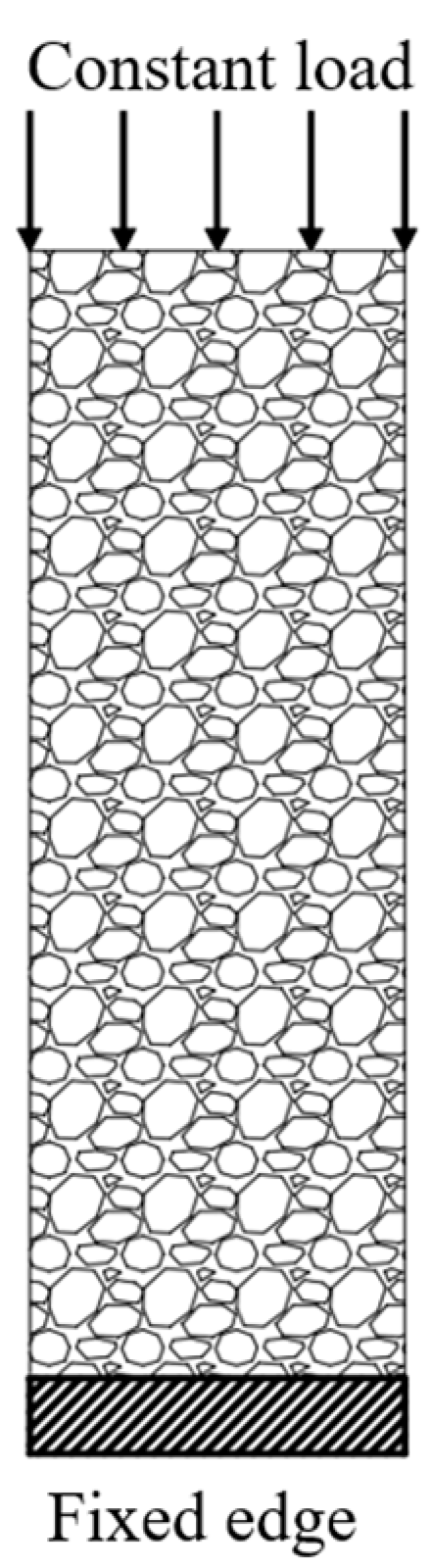
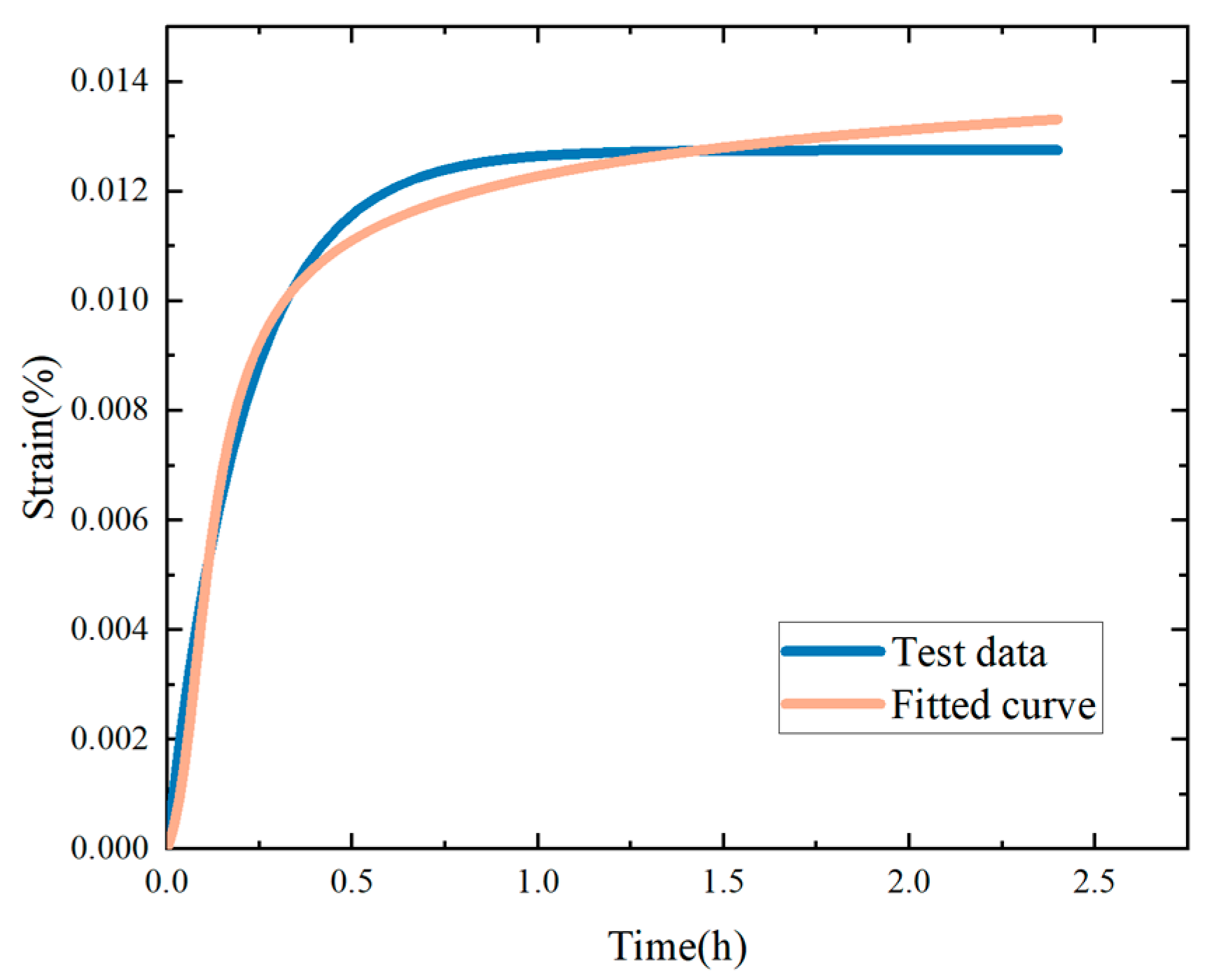
4.1. Simple Compression Creep Test of Sandstone

Liu et al. [10] conducted sandstone creep experiments. Samples were made as cylindrical shapes with a height of 100 mm and a diameter of 50 mm. The samples were subjected to uniform compression stress on the top edge, with the applied uniform force σ₀ = 39.4 MPa. Then, the creep curve was taken as the average of the test results. In this section, a simple compression numerical simulation of creep is conducted. The numerical results are compared with the test results to verify the validity of the VOTFK PD model proposed in this study. A 2D numerical specimen under plain strain conditions is established for simplification. Figure 6 shows the geometry and boundary conditions. The established coordinate system coincides with the geometric center of the model and is assumed to be positive in the vertical downward direction and positive in the horizontal rightward direction. The span of the material point is set as Δx = 2.5 mm. After uniform discretion, 20 material points are obtained in the x-direction and 40 material points in the y-direction. Consistent with the recommendation by the authors [40], we begin with a point-associated horizon size of δ = 3.0 Δx to strike a balance between computational cost and precision. The vertical displacement of the bottom region is fixed and the other boundaries are free to deform, while the vertical uniaxial compressive load is imposed on the top of the model. Displacement constraints are applied to the material points of the virtual boundary layer of thickness δ to ensure that the applied constraints are adequately reflected on the real material region. The external traction force is applied as a body force on a virtual boundary layer of thickness Δx. The y-direction displacement at the midpoint A on the top surface of the specimen is measured to obtain the axial creep strain curve. The vertical compressive load is instantaneously imposed on the top end of the specimen and is then held constant (σ₀ = 39.4 MPa) throughout the observation time interval. During the numerical iterations, the time integration is performed by adopting a real-time step size of Δt = 0.0012 h. The VOTFK PD model parameters, which are listed in

Table 1. Fitting parameters of proposed models for sandstone.

Model	E (MPa)	μ (MPa·s)	α
COTFK PD	68.1	9.6	0.12
VOTFK PD	72.3	9.3	e−9.50t

, are obtained by fitting the test results using Algorithm 1.

Algorithm 1. A Particle Method Levenberg–Marquardt Algorithm.

With the given initial data, the boundary information and the observation data $\theta$: Inputs:$\mathrm{Time} \mathrm{history} \mathrm{of} \mathrm{deflection} \mathrm{at} N_{\theta }$$\mathrm{sensor} \mathrm{locations}, X_s=\{x_{1,}{x}_2,\dots ,x_{N_{\theta }}\}$. Initialize the self-adaptive guess $p_0$$\mathrm{and} \mathrm{choose} \beta \in (0,1),\sigma (0,{\displaystyle \frac{1}{2}}),{\varsigma }_0>0$ and a $\delta$ small enough. for $k=1,\dots ,$ Iterations do $\mathrm{Solve} \mathrm{the} \mathrm{model} \mathrm{problem} \mathrm{corresponding} \mathrm{to} p_k$$\mathrm{and} p_k+\delta e_k$ respectively to obtain $\mathrm{the} \mathrm{data} u_h(\cdot ,p_k)$$\mathrm{and} u_h(\cdot ,p_k+\delta e_k)$. $\mathrm{Use} \mathrm{Formula} \left(43\right) \mathrm{to} \mathrm{numerically} \mathrm{compute} \mathrm{Jacobian} J_k$$\mathrm{and} J_k^T{r}_k$. Update the search   direction $d_k:=-{(J_k^T{J}_k+{\varsigma }_{k}I)}^{-1}{J}_k^T{r}_k.$ $\mathrm{Determine} \mathrm{the} \mathrm{search} \mathrm{step} {\beta }^m$ by the Armijo rule: find the smallest possible $m$   such that $ƛ(p_k+{\beta }^m{d}_k)\le ƛ(p_k)+\sigma {\beta }^m{d}_k{J}_k^T{r}_k.$ $\mathrm{If} \left|{\beta }^m{d}_k\right|\le$$\mathrm{Tolerance}, \mathrm{then} \mathrm{stop} \mathrm{and} \mathrm{let} p_{inv}:=p_k$. Otherwise update $p_{k+1}:=p_k+{\beta }^m{d}_k,$${\varsigma }_{k+1}:={\displaystyle \frac{{\varsigma }_k}{2}}$ and continue looping. end

These test data and the fitting constitutive curves via Algorithm 1 are plotted in Figure 7a, which shows a great agreement. The creep section of the numerical test is intercepted for comparison with the test to verify the properties of variable fractional order, comparing the curves of constant fractional order viscoelastic materials (Figure 7b). Obviously, the VOTFK PD can better accurately predict the creep curve compared to constant-order time-fractional Kelvin peridynamics (COTFK PD). The beginning of the creep curve cannot be accurately predicted due to the fact that that the spring must follow the slow deformation of the dashpot in the Kelvin model. This means that the proposed model is more suitable for describing the mechanical behavior of rock with a high initial viscosity.

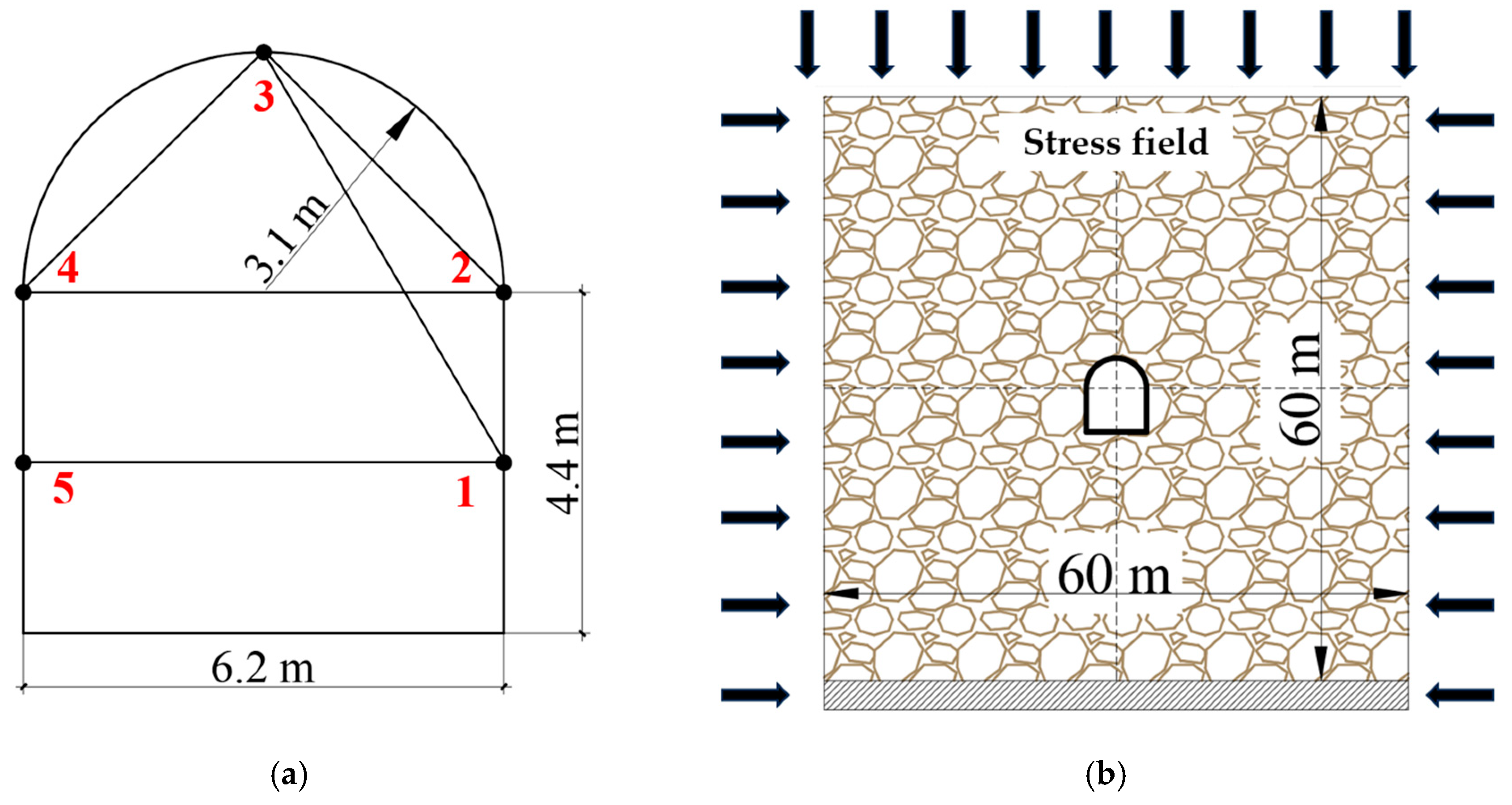
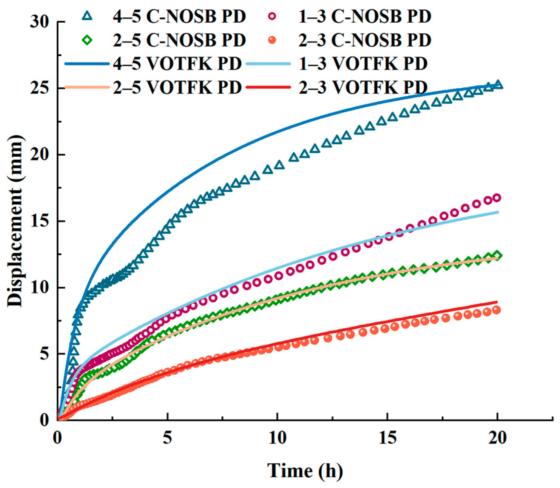
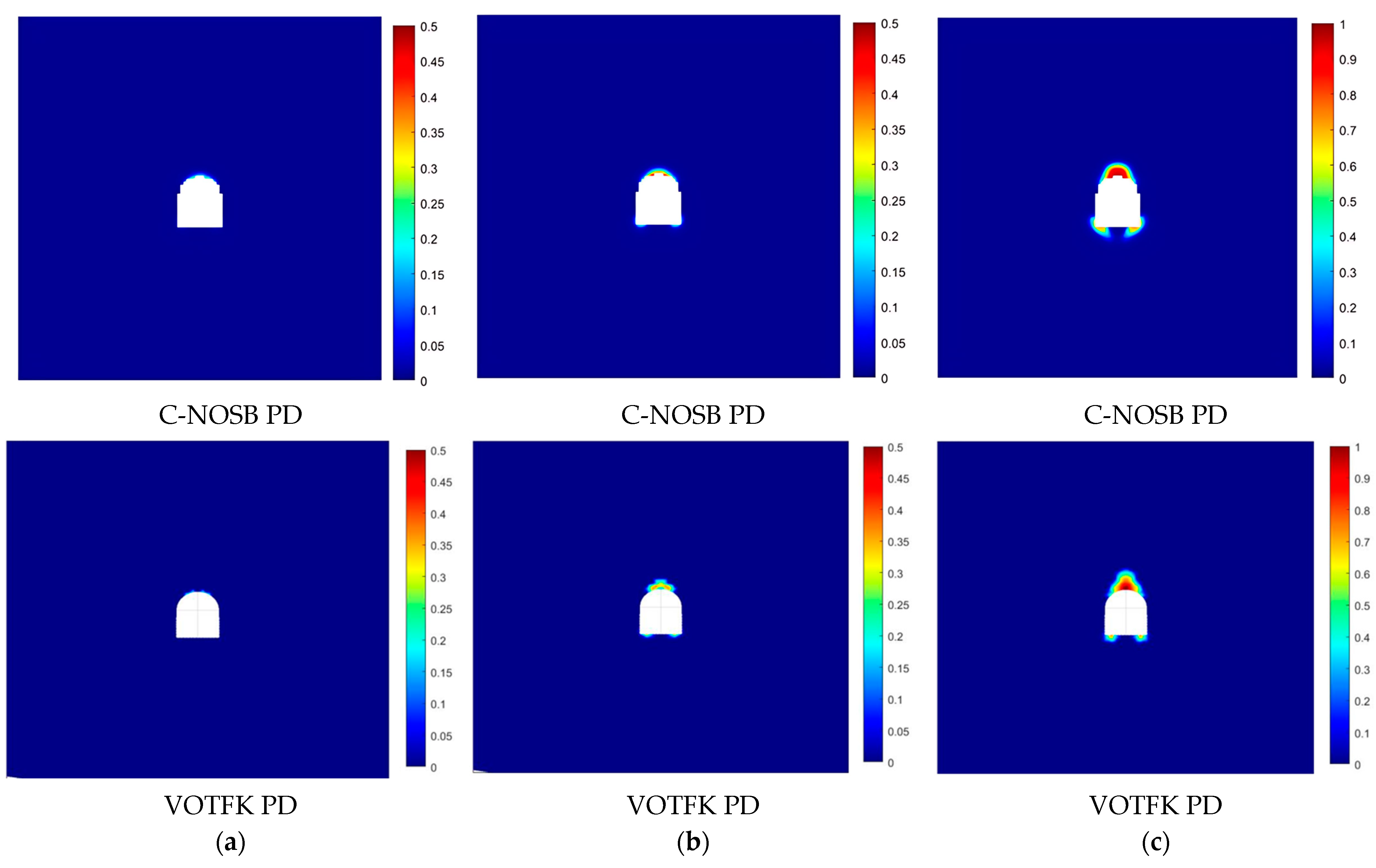
4.2. Numerical Test of Tunnel Rheology Behavior

To further evaluate the validity and correctness of the VOTFK PD model, the numerical test for practical engineering is carried out in this section. The proposed model is utilized to simulate the time-varying behavior after tunnel excavation, using the section of the auxiliary hole of the China Jinping secondary hydropower station as an example [41]. Similarly, a 2D numerical specimen under plain strain conditions is established. The cross-section geometry is shown in Figure 8a, and five monitoring points are arranged around the perimeter. The modeling area is centered on point O. The horizontal and vertical directions are taken as 60 m. The span of material point is set as Δx = 500 mm. After uniform discretion, 120 material points are obtained in one direction. The horizon size is set as δ = 3.0 Δx. According to the research of Chen et al. [42], the stress field is assumed as uniform and equal to 36.36 MPa. As shown in Figure 8b, horizontal and vertical displacement at the bottom is set as fixed, fixed lateral displacement is set at the left and right boundaries, and a free boundary is set at the top edge, applying normal compressive loads on the left, right, and top edges. Displacement constraints are applied to the material points of the virtual boundary layer of thickness δ to ensure that the applied constraints are adequately reflected on the real material region. The external traction force is applied as a body force on a virtual boundary layer of thickness Δx.

According to the research conducted by Chen et al. [42], the Kelvin–Voigt constitutive model of marble is expressed as

$$E_2^K\dot{\epsilon }+{\displaystyle \frac{E_1^K{E}_2^K}{{\mu }_1^K}}\epsilon =\dot{\sigma }+{\displaystyle \frac{E_1^K+E_2^K}{{\mu }_1^K}}\sigma$$

(43)

where the E₁^K= 20.97 GPa, E₂^K= 3.30 GPa, and μ₁^K= 4.39 GPa, according to test data. When the applied stress is constant (σ = 36.36 MPa), the equation transforms into

$${\sigma }_0={\displaystyle \frac{{\mu }_1^K}{E_1^K+E_2^K}}\left(E_2^K\dot{\epsilon }+{\displaystyle \frac{E_1^K{E}_2^K}{{\mu }_1^K}}\epsilon \right)$$

(44)

The corresponding creep curve is shown in Figure 9. Based on the Levenberg–Marquardt method, the VOTFK PD model parameters, which are listed in

Table 2. Fitting parameters of proposed models for marble.

E (MPa)	μ (MPa·h)	α
609.2	2772.1	e−15.1t

, can be determined. As seen, the fitting curve agrees well with the test creep curve in the initial stage, which again indicates that the proposed model is more suitable for describing the mechanical behavior of rock with a high initial viscosity. Moreover, for viscoelastic materials with a relatively low initial viscosity, as shown in Figure 7a, an additional spring element should be added to the Kelvin model to show the instantaneous elastic deformation [12].

During the numerical test, the deformation of survey lines based on five monitoring points is measured to obtain the deformation curves. To verify the accuracy of the model, the numerical results of the continuum-kinematic-inspired non-ordinary state-based peridynamics (C-NOSB PD) model proposed Tian et al. [40] are used for comparison. Note that the C-NOSB PD model was established as a constant-order time-fractional model. As seen, the calculation results of VTOFK PD for different survey lines are very close to the results of C-NOSB PD (Figure 10). These findings all validate the effectiveness and correctness of the proposed viscoelastic VTOFK PD model, which can accurately predict the time-varying behavior of rock. Gao et al. [4] presented the analytical results of a fractional order Burger model for the 4–5 line in the China Jinping secondary hydropower station. Hence, to quantitatively analyze the accuracy of the proposed model, the analytical results are employed to work as the reference to analyze the error of C-NOSB PD with respect to the proposed model. The maximum error between the C-NOSBPD model and the VOTFK PD model proposed in this paper is compared. As shown in Figure 11, when t = 2.92 d, the calculated displacement of C-NOSB PD is 5.38 mm and the calculated displacement of VOTFK PD is 6.28 mm, while the analytical result is 7.27 mm. It can be concluded that the accuracy is improved by 16.7%.

Table 3. Comparison of numerical results of VTOFK PD and test results.

Time (h)	Test Result (mm)	VTOFK PD (mm)	Error (%)
0.00	0.00	0.00	0.00
0.83	4.58	3.40	25.76
1.93	5.51	5.28	4.17
2.85	6.28	6.21	1.11
3.69	7.23	6.98	3.46
5.20	8.17	8.23	0.73
5.95	9.11	8.81	3.29
7.05	9.58	9.61	0.31
8.13	10.51	10.33	1.71
9.15	10.81	10.98	1.57
10.07	11.28	11.49	1.86
10.81	11.59	11.53	0.52
12.16	12.21	12.64	3.52
13.41	12.84	13.23	3.04
13.92	12.99	13.45	3.54
14.92	13.78	13.58	1.45
16.18	14.07	14.38	2.20
17.10	14.54	15.04	3.44
18.44	15.01	15.18	1.13
19.03	15.31	15.37	0.39
19.97	15.30	15.67	2.42
		Mean error	3.13

shows the comparison of the displacement of survey line 1–3 between test result [4] and the calculation result of VTOFK PD. Except for the initial stage, which has an error of 25.76%, the error of the rest of the moments is all lower than 4.2%, with an average error of 3.13%, proving that the proposed VOTFK PD model can accurately simulate the deformation behavior of rock at the engineering site.

Figure 12 presents a comparison of the evolution process of the damage zone over time during the rock creep process (after smoothing the cloud map), which is obtained by simulating using C-NOSB PD and VOTFK PD. The damage first appears at the top of the arch, and over time the accumulated damage caused by rock creep behavior at the top gradually expands. Damage areas also gradually appear at the left and right corners of the arch, and these damages continue to develop until the tunnel is destroyed. This damage evolution law is consistent with the general damage and failure mechanism of tunnels. This presents that the proposed model can adequately simulate the evolution of tunnel damage. Tian et al. [40] used a viscoelastic model with a larger number of components to achieve this damage simulation effect, while using a variable fractional order can achieve this effect with fewer parameters.

In conclusion, by comparison of displacement and damaged field, it can be found that by adjusting the fractional order parameter, the creep behavior of rock can be simulated with fewer model parameters.

5. Conclusions

In this paper, we propose a variable-order time-fractional Kelvin peridynamics model for accurately describing the time-dependent nonlinear creep deformation and failure behavior of rock, considering the consumption of viscosity during the creep process. Additionally, we present the L1 temporal discretization scheme to approximate the fractional-order derivative. Furthermore, a corresponding model parameter evaluation method based on Algorithm 1 is employed for practical applications. Numerical tests of rock creep show the utility of the developed method in practical applications.

Compared to constant-order time-fractional peridynamics, the proposed model improves the accuracy by 16.7% with fewer model parameters. Comparing to the test results, the calculation results of the proposed model have a mean error of 3.13%, except for the deformation error of 25.76% in the initial stage. It can be concluded that the proposed model can adequately simulate the deformation behavior of rock and the damage process in deformation, but the model is more suitable for describing the mechanical behavior of rock with a high initial viscosity.

References

1. Wang, Q.; Wang, Y.; Zan, Y.; Lu, W.; Bai, X.; Guo, J. Peridynamics simulation of the fragmentation of ice cover by blast loads of an underwater explosion. J. Mar. Sci. Technol. 2018, 23, 52–66. [Google Scholar] [CrossRef]
2. Xu, T.; Xu, Q.; Deng, M.; Ma, T.; Yang, T.; Tang, C.-A. A numerical analysis of rock creep-induced slide: A case study from Jiweishan Mountain, China. Environ. Earth Sci. 2014, 72, 2111–2128. [Google Scholar] [CrossRef]
3. Hou, Z.; Wundram, L.; Meyer, R.; Schmidt, M.; Schmitz, S.; Were, P. Development of a long-term wellbore sealing concept based on numerical simulations and in situ-testing in the Altmark natural gas field. Environ. Earth Sci. 2012, 67, 395–409. [Google Scholar] [CrossRef]
4. Gao, Y.H.; Zhou, Z.; Zhang, H.; Jin, S.; Yang, W.; Meng, Q.H. Viscoelastoplastic displacement solution for deep buried circular tunnel based on a fractional derivative creep model. Adv. Civ. Eng. 2021, 2021, 3664578. [Google Scholar] [CrossRef]
5. Wang, Y.; Liu, Y.; Li, Y.; Jiang, W.; Wang, Y. Experimental study on the failure mechanism of tunnel surrounding rock under different groundwater seepage paths. Geofluids 2021, 2021, 8856365. [Google Scholar] [CrossRef]
6. Yu, J.; Liu, G.; Cai, Y.; Zhou, J.; Liu, S.; Tu, B. Time-dependent deformation mechanism for swelling soft-rock tunnels in coal mines and its mathematical deduction. Int. J. Geomech. 2020, 20, 04019186. [Google Scholar] [CrossRef]
7. Koellerr, C. Applications of fractional calculus to the theory of viscoelasticity. J. Appl. Mech. 1984, 51, 299–307. [Google Scholar] [CrossRef]
8. Tian, D.L.; Zhou, X.P. The kinematic-constraint-inspired non-ordinary state-based peridynamics with fractional viscoelas-tic-viscoplastic constitutive model to simulating time-dependent deformation and failure of rocks. Comput. Methods Appl. Mech. Eng. 2024, 424, 116873. [Google Scholar] [CrossRef]
9. Yin, D.; Zhang, W.; Cheng, C.; Li, Y. Fractional time-dependent Bingham model for muddy clay. J. Non-Newton. Fluid. Mech. 2012, 187, 32–35. [Google Scholar] [CrossRef]
10. Liu, X.; Li, D. Nonlinear damage creep model based on variable-order fractional theory for rock materials. SN Appl. Sci. 2020, 2, 2029. [Google Scholar] [CrossRef]
11. Sun, H.G.; Chen, W.; Wei, H.; Chen, Y.Q. A comparative study of constant-order and variable-order fractional models in characterizing memory property of systems. Eur. Phys. J. Spec. Top. 2011, 193, 185–192. [Google Scholar] [CrossRef]
12. Liu, X.; Li, D.; Han, C.; Shao, Y. A Caputo variable-order fractional damage creep model for sandstone considering effect of relaxation time. Acta Geotech. 2022, 17, 153–167. [Google Scholar] [CrossRef]
13. Shin, J.H.; Potts, D.M.; Zdravkovic, L. The effect of pore-water pressure on NATM tunnel linings in decomposed granite soil. Can. Geotech. J. 2005, 42, 1585–1599. [Google Scholar] [CrossRef]
14. Wu, H.N.; Shen, S.L.; Chen, R.P.; Zhou, A. Three-dimensional numerical modelling on localised leakage in segmental lining of shield tunnels. Comput. Geotech. 2020, 122, 103549. [Google Scholar] [CrossRef]
15. Wang, Q.Y.; Zhu, W.C.; Xu, T.; Niu, L.L.; Wei, J. Numerical simulation of rock creep behavior with a damage-based constitutive law. Int. J. Geomech. 2017, 17, 04016044. [Google Scholar] [CrossRef]
16. Li, B.; Yu, H.; Ji, D.; Wang, F.; Lei, Z.; Wu, H. Pore-scale imbibition patterns in layered porous media with fractures. Phys. Fluids 2024, 36, 012120. [Google Scholar] [CrossRef]
17. Wang, C.; Liu, B.; Mohammadi, M.-R.; Fu, L.; Fattahi, E.; Motra, H.B.; Hazra, B.; Hemmati-Sarapardeh, A.; Ostadhassan, M. Integrating experimental study and intelligent modeling of pore evolution in the Bakken during simulated thermal progression for CO2 storage goals. Appl. Energy 2024, 359, 122693. [Google Scholar] [CrossRef]
18. Reddy, J.N. An Introduction to Continuum Mechanics; Cambridge University Press: Cambridge, UK, 2013. [Google Scholar]
19. Silling, S.A. Reformulation of elasticity theory for discontinuities and long-range forces. J. Mech. Phys. Solids 2000, 48, 175–209. [Google Scholar] [CrossRef]
20. Silling, S.A.; Askari, E. A meshfree method based on the peridynamic model of solid mechanics. Comput. Struct. 2005, 83, 1526–1535. [Google Scholar] [CrossRef]
21. Kilic, B.; Madenci, E. Prediction of crack paths in a quenched glass plate by using peridynamic theory. Int. J. Fract. 2009, 156, 165–177. [Google Scholar] [CrossRef]
22. Lai, X.; Ren, B.; Fan, H.; Li, S.; Wu, C.T.; Regueiro, R.A.; Liu, L. Peridynamics simulations of geomaterial fragmentation by impulse loads. Int. J. Numer. Anal. Methods Geomech. 2015, 39, 1304–1330. [Google Scholar]
23. Oterkus, E.; Madenci, E.; Weckner, O.; Silling, S.; Bogert, P.; Tessler, A. Combined finite element and peridynamic analyses for predicting failure in a stiffened composite curved panel with a central slot. Compos. Struct. 2012, 94, 839–850. [Google Scholar]
24. Weckner, O.; Mohamed, N.A.N. Viscoelastic material models in peridynamics. Appl. Math. Comput. 2013, 219, 6039–6043. [Google Scholar] [CrossRef]
25. Ha, Y.D.; Lee, J.; Hong, J.W. Fracturing patterns of rock-like materials in compression captured with peridynamics. Eng. Fract. Mech. 2015, 144, 176–193. [Google Scholar]
26. Zhou, X.P.; Shou, Y.D. Numerical simulation of failure of rock-like material subjected to compressive loads using improved peridynamic method. Int. J. Geomech. 2017, 17, 04016086. [Google Scholar] [CrossRef]
27. Mainardi, F. Fractional Calculus and Waves in Linear Viscoelasticity: An Introduction to Mathematical Models; World Scientific: Singapore, 2022. [Google Scholar]
28. Farno, E.; Baudez, J.-C.; Eshtiaghi, N. Comparison between classical Kelvin-Voigt and fractional derivative Kelvin-Voigt models in prediction of linear viscoelastic behaviour of waste activated sludge. Sci. Total Environ. 2018, 613, 1031–1036. [Google Scholar] [PubMed]
29. Gao, C.; Zhou, Z.; Li, Z.; Li, L.; Cheng, S. Peridynamics simulation of surrounding rock damage characteristics during tunnel excavation. Tunn. Undergr. Space Technol. 2020, 97, 103289. [Google Scholar]
30. Zaky, M.; Hendy, A.; Suragan, D. A note on a class of Caputo fractional differential equations with respect to another function. Math. Comput. Simul. 2022, 196, 289–295. [Google Scholar] [CrossRef]
31. Suzuki, J.L.; Kharazmi, E.; Varghaei, P.; Naghibolhosseini, M.; Zayernouri, M. Anomalous nonlinear dynamics behavior of fractional viscoelastic beams. J. Comput. Nonlinear Dyn. 2021, 16, 111005. [Google Scholar]
32. Zheng, X.; Wang, H. A hidden-memory variable-order time-fractional optimal control model: Analysis and approximation. SIAM J. Control Optim. 2021, 59, 1851–1880. [Google Scholar]
33. Benson, D.A.; Schumer, R.; Meerschaert, M.M.; Wheatcraft, S.W. Fractional dispersion, Lévy motion, and the MADE tracer tests. Transp. Porous Media 2001, 42, 211–240. [Google Scholar]
34. Pang, G.; Lu, L.; Karniadakis, G.E. fPINNs: Fractional physics-informed neural networks. SIAM J. Sci. Comput. 2019, 41, A2603–A2626. [Google Scholar]
35. Zayernouri, M.; Karniadakis, G.E. Fractional spectral collocation methods for linear and nonlinear variable order FPDEs. J. Comput. Phys. 2015, 293, 312–338. [Google Scholar]
36. Kilic, B.; Madenci, E. An adaptive dynamic relaxation method for quasi-static simulations using the peridynamic theory. Theor. Appl. Fract. Mech. 2010, 53, 194–204. [Google Scholar]
37. Underwood, P. Dynamic Relaxation, in: Computational Method for Transient Analysis. Chapter 1983, 5, 245–256. [Google Scholar]
38. Foster, J.T.; Silling, S.A.; Chen, W.W. Viscoplasticity using peridynamics. Int. J. Numer. Methods Eng. 2010, 81, 1242–1258. [Google Scholar]
39. Parks, M.L.; Lehoucq, R.B.; Plimpton, S.J.; Silling, S.A. Implementing peridynamics within a molecular dynamics code. Comput. Phys. Commun. 2008, 179, 777–783. [Google Scholar]
40. Tian, D.L.; Zhou, X.P. A novel kinematic-constraint-inspired non-ordinary state-based peridynamics. Appl. Math. Model. 2022, 109, 709–740. [Google Scholar]
41. Javili, A.; Ekiz, E.; McBride, A.T.; Steinmann, P. Continuum-kinematics-inspired peridynamics: Thermo-mechanical problems. Contin. Mech. Thermodyn. 2021, 33, 2039–2063. [Google Scholar]
42. Chen, B.R.; Feng, X. Universal viscoelastoplastic combination model and its engineering applications. Chin. J. Rock. Mech. Eng. 2008, 27, 1028–1035. [Google Scholar]
Figure 1. Schematic illustration of the intricate creep behavior of rocks.
Fractalfract 09 00197 g001
Figure 2. Bond-based peridynamics.
Fractalfract 09 00197 g002
Figure 3. Sketch of the Kelvin creep model.
Fractalfract 09 00197 g003
Figure 4. Creep curve of Abel dashpot.
Fractalfract 09 00197 g004
Figure 5. Integral domain and volume correction (the pink region of the material point is in the horizon area while the blue region is not in the horizon area).
Fractalfract 09 00197 g005
Figure 6. Samples’ geometry and compression loading.
Fractalfract 09 00197 g006
Figure 7. Comparison of numerical test and test data. (a) Fitting curve; (b) numerical results.
Fractalfract 09 00197 g007
Figure 8. Test setup. (a) Layout of tunnel cross section; (b) geometry and boundary conditions of study zone.
Fractalfract 09 00197 g008
Figure 9. Fitting creep curve of marble.
Fractalfract 09 00197 g009
Figure 10. Comparison of deformation of measuring line with time for the C-NOSB PD and VOTFK PD models.
Fractalfract 09 00197 g010
Figure 11. Comparison of the deformation along the survey line over time for the analytical solution, C-NOSB PD, and VOTFK PD.
Fractalfract 09 00197 g011
Figure 12. Comparison of the evolution of damaged zone. (a) t = 10.5 d; (b) t = 17.5 d; (c) t = 21 d.
Fractalfract 09 00197 g012