


Applying Two Fractional Methods for Studying a Novel General Formula of Delayed-Neutron-Affected Nuclear Reactor Equations

Abstract
1. Introduction
2. The Physical Phenomena
3. Preliminaries
- (i)
- ;
- (ii)
- ;
- (iii)
- ;
- (iv)
- ;
- (v)
- , and .
4. Methods Principal Ideas
4.1. The Fractional TAM
4.2. The Fractional SRPSM
5. Neutron Diffusion Equations Analytical Solutions
5.1. Analytical Solution by TAM
5.2. Analytical Solution by SRPSM
6. Numerical Study
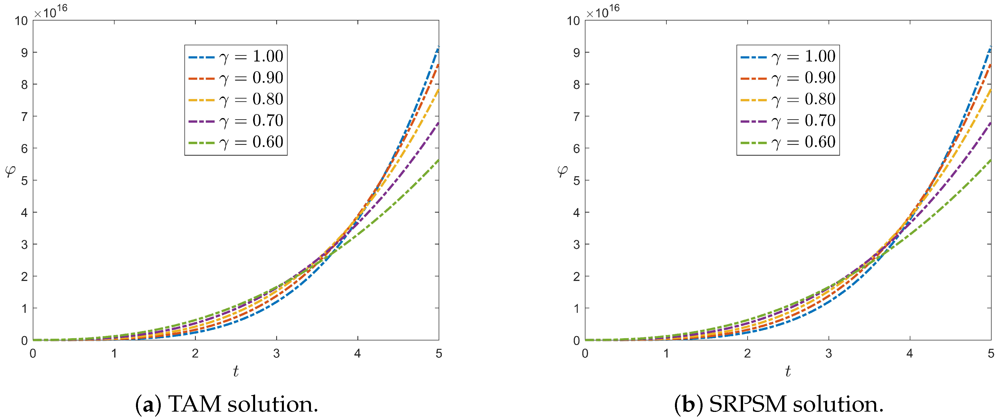
6.1. Slab Reactor
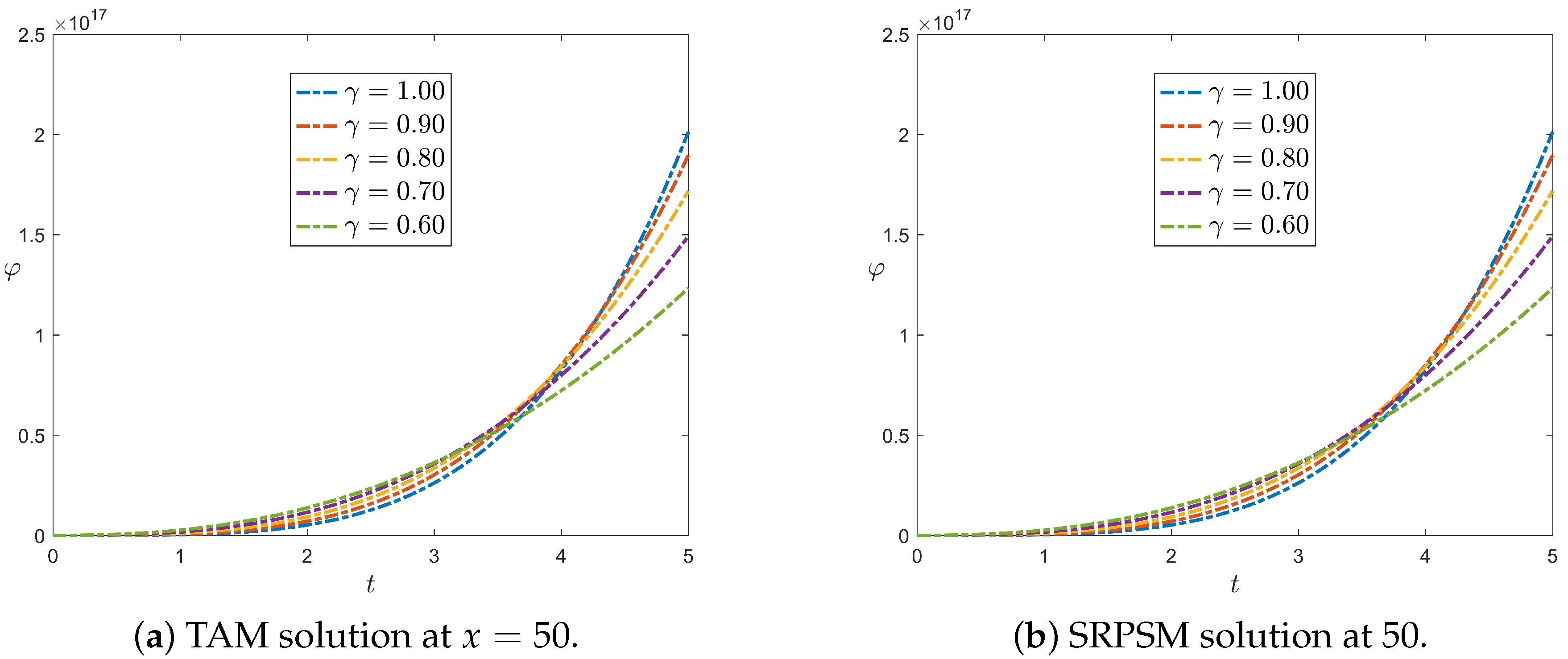
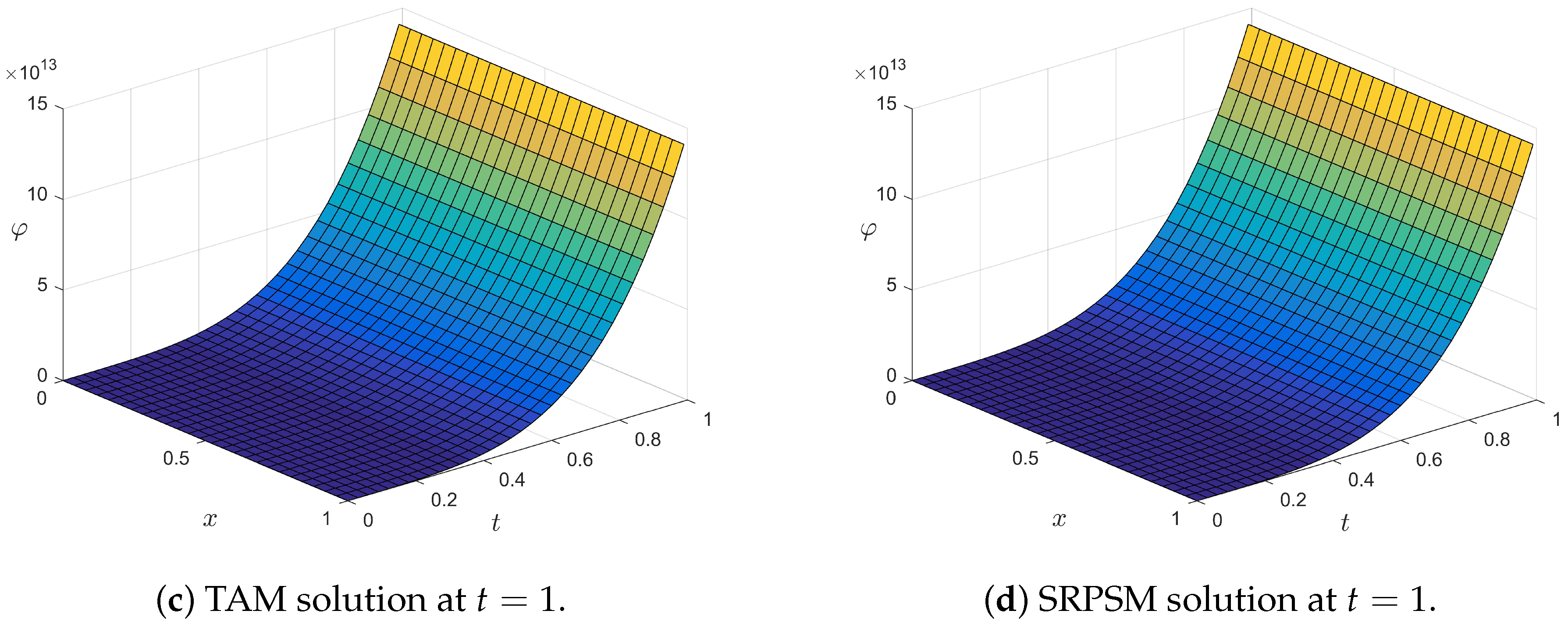
6.2. Infinite Cylindrical Reactor
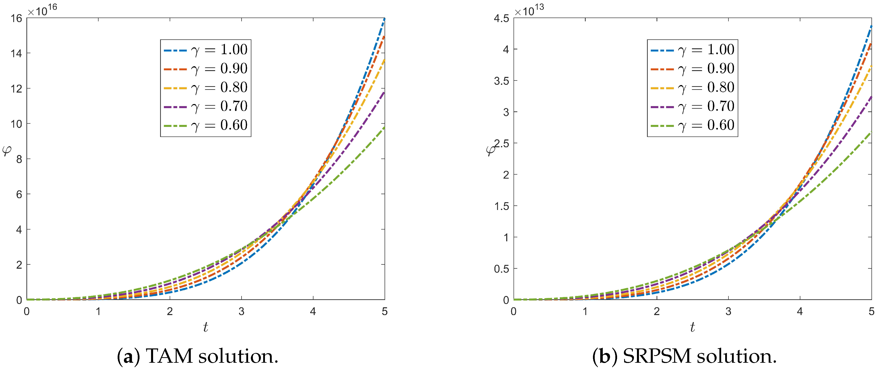
6.3. Spherical Reactor
6.4. Computational Performance of TAM and SRPSM
7. Conclusions
Author Contributions
Funding
Data Availability Statement
Conflicts of Interest
References
- Lee, J.C. Nuclear Reactor: Physics and Engineering; John Wiley and Sons: Hoboken, NJ, USA, 2020. [Google Scholar]
- Stacey, W.M. Nuclear Reactor Physics; John Wiley and Sons: Hoboken, NJ, USA, 2018. [Google Scholar]
- Almenas, K.; Lee, R. Nuclear Engineering: An Introduction; Springer Science and Business Media: Berlin/Heidelberg, Germany, 2012. [Google Scholar]
- Heyde, K. Basic Ideas and Concepts in Nuclear Physics: An Introductory Approach; CRC Press: Boca Raton, FL, USA, 2020. [Google Scholar]
- Cassell, J.S.; Williams, M.M. A solution of the neutron diffusion equation for a hemisphere with mixed boundary conditions. Ann. Nucl. Energy 2004, 31, 1987–2004. [Google Scholar] [CrossRef]
- Williams, M.M. Neutron transport in two interacting slabs II: The influence of transverse leakage. Ann. Nucl. Energy 2002, 29, 1551–1596. [Google Scholar] [CrossRef]
- Khasawneh, K.; Dababneh, S.; Odibat, Z. A solution of the neutron diffusion equation in hemispherical symmetry using the homotopy perturbation method. Ann. Nucl. Energy 2009, 36, 1711–1717. [Google Scholar] [CrossRef]
- Dababneh, S.; Khasawneh, K.; Odibat, Z. An alternative solution of the neutron diffusion equation in cylindrical symmetry. Ann. Nucl. Energy 2011, 38, 1140–1143. [Google Scholar] [CrossRef]
- El-Ajou, A.; Shqair, M.; Ghabar, I.; Burqan, A.; Saadeh, R. A solution for the neutron diffusion equation in the spherical and hemispherical reactors using the residual power series. Front. Phys. 2023, 11, 1229142. [Google Scholar] [CrossRef]
- Filali, D.; Shqair, M.; Alghamdi, F.A.; Ismaeel, S.; Hagag, A. Solving a Novel System of Time-Dependent Nuclear Reactor Equations of Fractional Order. Symmetry 2024, 16, 831. [Google Scholar] [CrossRef]
- Roul, P.; Rohil, V.; Espinosa-Paredes, G.; Obaidurrahman, K. Numerical approximation of a two-dimensional fractional neutron diffusion model describing dynamics of neutron flux in a nuclear reactor. Prog. Nucl. Energy 2024, 172, 105212. [Google Scholar] [CrossRef]
- Aboanber, A.E.; Nahla, A.A.; Aljawazneh, S.M. Fractional two energy groups matrix representation for nuclear reactor dynamics with an external source. Ann. Nucl. Energy 2021, 153, 108062. [Google Scholar] [CrossRef]
- Sardar, T.; Saha Ray, S.; Bera, R.K.; Biswas, B.B.; Das, S. The solution of coupled fractional neutron diffusion equations with delayed neutrons. Int. J. Nucl. Energy Sci. Technol. 2010, 5, 105–113. [Google Scholar] [CrossRef]
- Khaled, S.M. Exact solution of the one-dimensional neutron diffusion kinetic equation with one delayed precursor concentration in Cartesian geometry. AIMS Math. 2022, 7, 12364–12373. [Google Scholar] [CrossRef]
- Vázquez-Rodríguez, R.; Sánchez-Mora, H.; Polo-Labarrios, M.A.; Ortiz-Villafuerte, J.; Lugo-Leyte, R. Fractional neutron point kinetics model for reactivity transients of the NuScale and comparison with the classical kinetics approach. Prog. Nucl. Energy 2024, 105350, 0149–1970. [Google Scholar] [CrossRef]
- Yin, D.; Xie, Y.; Mei, L. The stability and convergence analysis of finite difference methods for the fractional neutron diffusion equation. Adv. Comput. Math. 2023, 49, 72. [Google Scholar] [CrossRef]
- Burqan, A. A Novel Scheme of the ARA Transform for Solving Systems of Partial Fractional Differential Equations. Fractal Fract. 2023, 7, 306. [Google Scholar] [CrossRef]
- Alia, A.; Abbasb, M.; Akramc, T. New group iterative schemes for solving the two-dimensional anomalous fractional sub-diffusion equation. J. Math. Comp. Sci. 2021, 22, 119–127. [Google Scholar] [CrossRef]
- Momani, S.; Shqair, M.; Batiha, I.; Abu-Sei’leek, M.H.; Alshorm, S.; Abd El-Azeem, S.A. Two Energy groups Neutron Diffusion Model in Spherical Reactors. Results Nonlinear Anal. 2024, 7, 160–173. [Google Scholar]
- Zhang, Q.; Liu, L.; Zhang, C. Compact scheme for fractional diffusion-wave equation with spatial variable coefficient and delays. Appl. Anal. 2022, 101, 1911–1932. [Google Scholar] [CrossRef]
- Ashyralyev, A.; Agirseven, D. On convergence of difference schemes for delay parabolic equations. Comput. Math. Appl. 2013, 66, 1232–1244. [Google Scholar] [CrossRef]
- Xie, J.; Zhang, Z. The high-order multistep ADI solver for two-dimensional nonlinear delayed reaction diffusion equations with variable coefficients. Comput. Math. Appl. 2018, 75, 3558–3570. [Google Scholar] [CrossRef]
- Temimi, H.; Ansari, A.R. A new iterative technique for solving nonlinear second order multi-point boundary value problems. Appl. Math. Comput. 2011, 218, 1457–1466. [Google Scholar] [CrossRef]
- Al-Hanaya, A.; Alotaibi, M.; Shqair, M.; Hagag, A.E. MHD effects on Casson fluid flow squeezing between parallel plates. AIMS Math. 2023, 8, 29440–29452. [Google Scholar] [CrossRef]
- Adwan, M.I.; Al-Jawary, M.A.; Tibaut, J.; Ravnik, J. Analytic and numerical solutions for linear and nonlinear multidimensional wave equations. Arab. J. Basic Appl. Sci. 2020, 27, 166–182. [Google Scholar] [CrossRef]
- Rao, A.; Vats, R.K.; Yadav, S. Numerical study of nonlinear time-fractional Caudrey Dodd Gibbon Sawada Kotera equation arising in propagation of waves. Chaos Solitons Fractals 2024, 184, 114941. [Google Scholar] [CrossRef]
- Nadeem, M.; Alsayaad, Y. Analytical study of one dimensional time fractional Schrodinger problems arising in quantum mechanics. Sci. Rep. 2024, 14, 12503. [Google Scholar] [CrossRef] [PubMed]
- Burqan, A.; Shqair, M.; El-Ajou, A.; Ismaeel, S.M.; Al-Zhour, Z. Analytical solutions to the coupled fractional neutron diffusion equations with delayed neutrons system using Laplace transform method. AIMS Math. 2023, 8, 19297–192312. [Google Scholar] [CrossRef]


| B | D | ∑ | ||
|---|---|---|---|---|
| 220 cm/s | 0.000735 cm−1 | 0.356 cm2/s | 0.08 s−1 | 0.005 cm−2 |
| Slab Reactor | Cylindrical Reactor | Spherical Reactor | ||||||
|---|---|---|---|---|---|---|---|---|
| x | [28] | [10] | ||||||
| 0.0 | 17.6177 | 17.6216 | 17.6212 | 67.1058 | 67.1205 | 67.1205 | 116.594 | 116.619 |
| 0.1 | 17.6291 | 17.6329 | 17.6253 | 67.1171 | 67.1318 | 67.1318 | 116.605 | 116.631 |
| 0.2 | 17.6631 | 17.6669 | 17.6677 | 67.1511 | 67.1658 | 67.1658 | 116.639 | 116.665 |
| 0.3 | 17.7197 | 17.7236 | 17.7227 | 67.2078 | 67.2225 | 67.2225 | 116.696 | 116.721 |
| 0.4 | 17.7991 | 17.8029 | 17.8011 | 67.2871 | 67.3018 | 67.3018 | 116.775 | 116.801 |
| 0.5 | 17.9011 | 17.9049 | 17.9035 | 67.3891 | 67.4038 | 67.4038 | 116.877 | 116.903 |
| 0.6 | 18.0257 | 18.0296 | 18.0290 | 67.5138 | 67.5285 | 67.5285 | 117.002 | 117.027 |
| 0.7 | 18.1731 | 18.1769 | 18.1766 | 67.6611 | 67.6758 | 67.6758 | 117.149 | 117.175 |
| 0.8 | 18.3431 | 18.3470 | 18.3398 | 67.8311 | 67.8458 | 67.8458 | 117.319 | 117.345 |
| 0.9 | 18.5358 | 18.5396 | 18.5412 | 68.0238 | 68.0385 | 68.0385 | 117.512 | 117.537 |
| 1.0 | 18.7511 | 18.7550 | 18.7495 | 68.2391 | 68.2538 | 68.2538 | 117.727 | 117.753 |
| Geometry | Method | CPU Time (s), | CPU Time (s), |
|---|---|---|---|
| Slab Reactor | TAM | 0.45 | 0.52 |
| SRPSM | 0.38 | 0.44 | |
| Cylindrical Reactor | TAM | 0.48 | 0.55 |
| SRPSM | 0.40 | 0.46 | |
| Spherical Reactor | TAM | 0.50 | 0.58 |
| SRPSM | 0.42 | 0.48 |
Disclaimer/Publisher’s Note: The statements, opinions and data contained in all publications are solely those of the individual author(s) and contributor(s) and not of MDPI and/or the editor(s). MDPI and/or the editor(s) disclaim responsibility for any injury to people or property resulting from any ideas, methods, instructions or products referred to in the content. |
© 2025 by the authors. Licensee MDPI, Basel, Switzerland. This article is an open access article distributed under the terms and conditions of the Creative Commons Attribution (CC BY) license (https://creativecommons.org/licenses/by/4.0/).
Share and Cite
Shqair, M.; Alqahtani, Z.; Hagag, A. Applying Two Fractional Methods for Studying a Novel General Formula of Delayed-Neutron-Affected Nuclear Reactor Equations. Fractal Fract. 2025, 9, 246. https://doi.org/10.3390/fractalfract9040246
Shqair M, Alqahtani Z, Hagag A. Applying Two Fractional Methods for Studying a Novel General Formula of Delayed-Neutron-Affected Nuclear Reactor Equations. Fractal and Fractional. 2025; 9(4):246. https://doi.org/10.3390/fractalfract9040246
Chicago/Turabian StyleShqair, Mohammed, Zuhur Alqahtani, and Ahmed Hagag. 2025. "Applying Two Fractional Methods for Studying a Novel General Formula of Delayed-Neutron-Affected Nuclear Reactor Equations" Fractal and Fractional 9, no. 4: 246. https://doi.org/10.3390/fractalfract9040246
APA StyleShqair, M., Alqahtani, Z., & Hagag, A. (2025). Applying Two Fractional Methods for Studying a Novel General Formula of Delayed-Neutron-Affected Nuclear Reactor Equations. Fractal and Fractional, 9(4), 246. https://doi.org/10.3390/fractalfract9040246