Abstract
In this research article, we investigate a three-dimensional dynamical system governed by fractal-fractional-order evolution differential equations subject to terminal boundary conditions. We derive existence and uniqueness results using Schaefer’s and Banach’s fixed-point theorems, respectively. Additionally, the Hyers–Ulam stability approach is employed to analyze the system’s stability. We employ vector terminology for the proposed problem to make the analysis simple. To illustrate the practical relevance of our findings, we apply the derived results to a numerical example and graphically illustrate the solution for different fractal-fractional orders, emphasizing the effect of the derivative’s order on system behavior.
1. Introduction
Fractional differential equations (FDEs) have gained considerable attention in recent decades due to their wide-ranging applications in both theoretical and practical fields. The interplay between the mathematical theory and real-world applications of fractional calculus has led to substantial advancements, positioning FDEs as a well-established field with diverse applications across physics, engineering, and technology. Their relevance spans control theory, electrochemistry, electromagnetics, viscoelasticity, and porous media, among others (see [1,2,3]). For further developments in this area, readers may consult [4,5,6].
Various fractional differential operators have been introduced to address different modeling scenarios. Among them, the fractal-fractional differential operator, classified as a special local fractional derivative [7], has gained prominence. This operator is a non-Newtonian modification of the classical derivative, specifically designed for fractal structures. Currently, fractal-fractional differential equations (FFDEs) are of great interest due to their applicability in modeling complex systems such as water permeation in wool fibers, multi-scale fabrics, and heat transfer [8]. Akgül [9] examined FFDEs with a power-law kernel, demonstrating their novel applications. Several recent studies have further expanded the utility of these concepts (see [10,11,12,13]).
Terminal value problems (TVPs) play a crucial role in modeling phenomena across various domains of physics and engineering. These problems naturally arise in retrospective simulations, where system states are analyzed from final conditions. These problems commonly arise in the mathematical modeling of numerous physical phenomena, including microscale heat transport and the hydrodynamics of liquid helium (see [14]). Furthermore, TBV problems form a subclass of differential equations and play an important role in nonlinear field theory, hydrodynamics, and particularly in the analysis of symmetric bubble-type solutions within the framework of shell-like theory (see [15]). The study of solution existence for classical TVPs has been extensively explored (see [16,17]), yet extending these results to fractional-order TVPs remains a more complex challenge. Diethelm [18] investigated the existence and stability properties of fractional TVPs on finite intervals, highlighting structural differences between initial and terminal value problems. In [19], Shiri et al. studied terminal value problems for nonlinear systems of FDEs. In [20], Ford et al. investigated high order numerical methods for fractional TVPs. In [21], Boichuk et al. studied TVPs for the system of FDEs incorporated additional restrictions. In [22], Bao et al. investigated existence and regularity results for TVP for nonlinear fractional wave equations.
Evolution equations are fundamental in real-world applications. Constructing solutions based on given initial or boundary conditions is a characteristic feature of these equations, making them essential in mathematical modeling. To ensure self-consistency in modeling real-world systems, it is crucial to establish the existence and uniqueness of solutions for evolution equations subject to initial or terminal boundary conditions. These equations are widely employed in areas such as acoustics, neural networks, and natural sciences. Numerous significant results have been reported for evolution equations using classical and fractional calculus techniques (see [23,24]).
Recently, fractal-fractional calculus has gained increasing attention due to its ability to model complex physical systems. Although the concept of fractals predates fractional calculus, fractal-fractional calculus has emerged as a powerful tool for studying real-world phenomena (see [25,26,27]). Notable applications include epidemiological modeling [28,29]. The proper investigation of evolution equations with terminal boundary conditions is necessary for establishing their solution existence, uniqueness, and stability. Additionally, triply coupled differential equation systems have been widely studied due to their relevance in numerous applications [30,31].
Motivated by the aforementioned study, we consider a three-dimensional system of fractal-fractional-order evolution differential equations with terminal boundary conditions:
where are fractal dimensions, and are the orders of the fractional derivative. The functions are continuous real functions dependent on x. The functions are nonlinear and continuous, the functions represent state variables of the system, and ; (i = 1, 2, 3) are real numbers.
Fractal-fractional calculus incorporates both fractional-order and fractal properties, allowing for a more accurate representation of memory-dependent systems. To the best of our knowledge, such problems have not been investigated yet using fractal-fractional calculus.
To simplify the notation, we employ vector terminology for the proposed problem as employed in [19]. Let
and
The system can now be written in vector form as:
where
This vector form can simplify the notation and make it easier to analyze and solve the system.
The manuscript is structured as follows: In Section 2, we provide the basic definitions and preliminary results. In Section 3, we establish the existence of solutions for the proposed problem. In Section 4, we analyze the stability of the proposed problem. In Section 5, we apply the main results to a general problem and present graphical representations of the solutions for various fractal and fractional orders, demonstrating the effectiveness of the proposed method. In Section 6, we conclude with a summary of the derived results.
2. Elementary Results
In this section, we present definitions of the fractal-fractional-order integral and derivative as well as some other basic definitions. Moreover, we provide a result and its proof that serve as a basis for subsequent analysis.
Definition 1
([25]). Let ϕ be a matrix of continuous functions and fractal differentiable on the open interval . Then, the fractal-fractional integral of with a power-law kernel is defined by
Definition 2
([25]). Let ϕ be a matrix of continuous functions and fractal differentiable on the open interval . Then, for the fractal-fractional Caputo derivative with a power-law kernel is defined as
Definition 3
([32,33]). A set G is equi-continuous on a domain D if for every there exists a positive number such that for all and for all satisfying , the following holds:
This concept can be extended to operators as follows:
Definition 4.
An operator mapping a normed space X into another normed space Y is termed equi-continuous if, for every exists such that all satisfying ; thus, we have:
Definition 5
([34]). An operator acting between normed spaces is called completely continuous if it is continuous and maps every bounded subset of X to relatively compact subsets of Y.
Theorem 1
([35]). Let be a non-empty, a closed subset of a Banach space X. If the mapping is a contraction, then has a unique fixed point.
Theorem 2
([36]). Suppose W is a normed linear space and is a convex subset of W that contains 0. If is a completely continuous operator, then either the set is unbounded or has a fixed point in .
Lemma 1.
Consider . Then, is the solution of the proposed problem:
if and only if it is the solution of the following integral equation:
Proof.
Assume that satisfies (6). Then,
Applying the fractal-fractional integral on both sides, we have
Since is the left inverse of we obtain
By putting we have
This equation satisfies (7).
In view of Lemma 1, we give the following definition.
3. Existence of Solutions
In this section, we investigate the existence of solutions for the problem under consideration. Since we are studying our problem within a Banach space, we first introduce a suitable Banach space as follows:
We define the space equipped with the following norm:
where Then, is a Banach space.
Define an operator by
For deriving the main results, we impose the following assumptions:
- ()
- Assume that the nonlinear functions are continuous.
- ()
- Assume that is a matrix of continuous real functions such that for some and for all i = 1, 2, 3.
- ()
- Assume that for any and for all such that the following relations hold:
- ()
- For all we have
Theorem 3.
Proof.
For arbitrary we consider
Using assumptions ()–(), we have
Consider the integral . Let This implies that If , then , and if , then . Thus, we have
where is a beta function. Similarly, the integral can be transformed by:
Hence from (18), we have
Since the operator is contraction. Therefore, by Banach’s Theorem, has exactly one fixed point. This proves the required result. □
Theorem 4.
Proof.
To investigate this result, we employ Shaefer’s fixed-point theorem. By (), the vector function is continuous and, therefore, the operator is is continuous. For to be completely continuous, it is necessary that
- It maps bounded sets of into bounded sets of ,
- It is equi-continuous.
Let a number exist such that the elements of the following defined set are upper bounded by it. We define a set is closed, bounded, and a convex subset of U, which is proved in the following steps.
- :
- is bounded.
For arbitrary we have
Taking the maximum and using the given assumptions, we have
Hence, is bounded.
- :
- is equi-continuous.
Let such that (s.t) . Then,
We see that right hand side of (27) tends to zero as . Consequently,
Thus, the operator is equi-continuous.
Also, by condition , is uniformly bounded. Consequently, the family is a relatively compact subset of U. Thus, is completely continuous. Therefore, by Schaefer’s fixed-point theorem, has a fixed point in □
4. Stability Analysis
In this section, we perform a Hyers–Ulam stability analysis for the triply coupled system of DEs (2). Let . Then, for we construct the inequality in the unknown function as follows:
where
The following Definitions 7 and 8 have been adapted from [37].
Definition 7.
Definition 8.
We make the following remark to obtain the corresponding perturbed problem with small perturbation functions. This remark is used to establish bounds on the perturbation’s effect on the system and to quantify the relationship between the perturbation and the resulting change in the system’s behavior.
Remark 1.
is a solution of the inequality (29), if there is a function that is dependent on such that for we have
By Remark 1, the following problem with small perturbation function is given:
Lemma 2.
Proof.
The proof is easy, so we omit it. □
Theorem 5.
Proof.
Let be any solution of the inequality (29), and let be the unique solution of problem (2). Then, from (7) and (33), we have
Simplifying further, we have
This shows that problem (2) is H-U stable. □
Corollary 1.
5. Illustrative Problem
In this section, we illustrate the applicability of our obtained results. We assign specific values to functions, fractional orders, fractal dimensions, and initial conditions in the proposed problem (2) as given bellow.
Example 1.
Let
From the vector function we have
For arbitrary we have
This implies that
Similarly,
Also,
For we derive
Hence, We see that conditions of Theorems 3 and 5 hold. Therefore, problem (37) has a unique solution that is H-U stable.
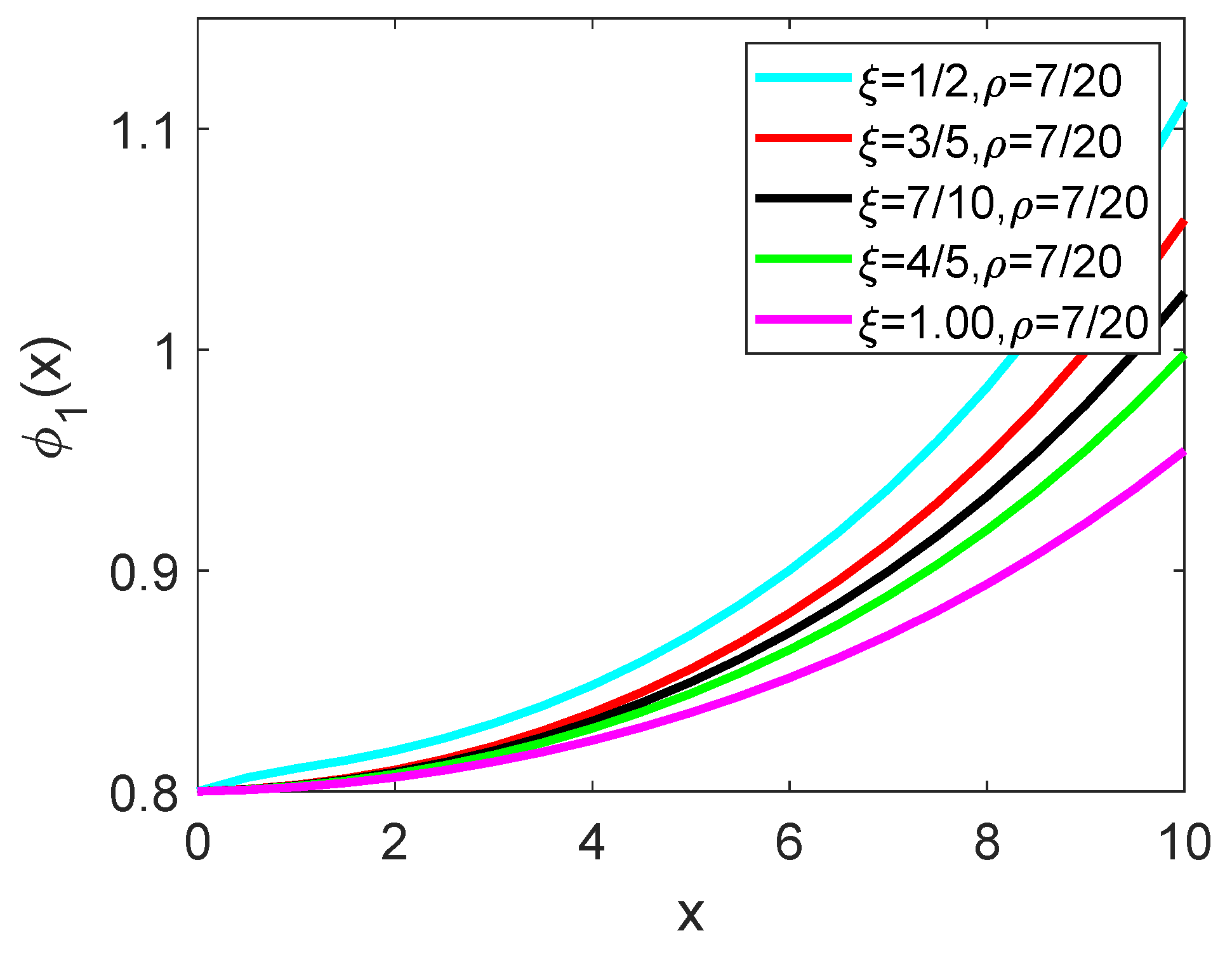
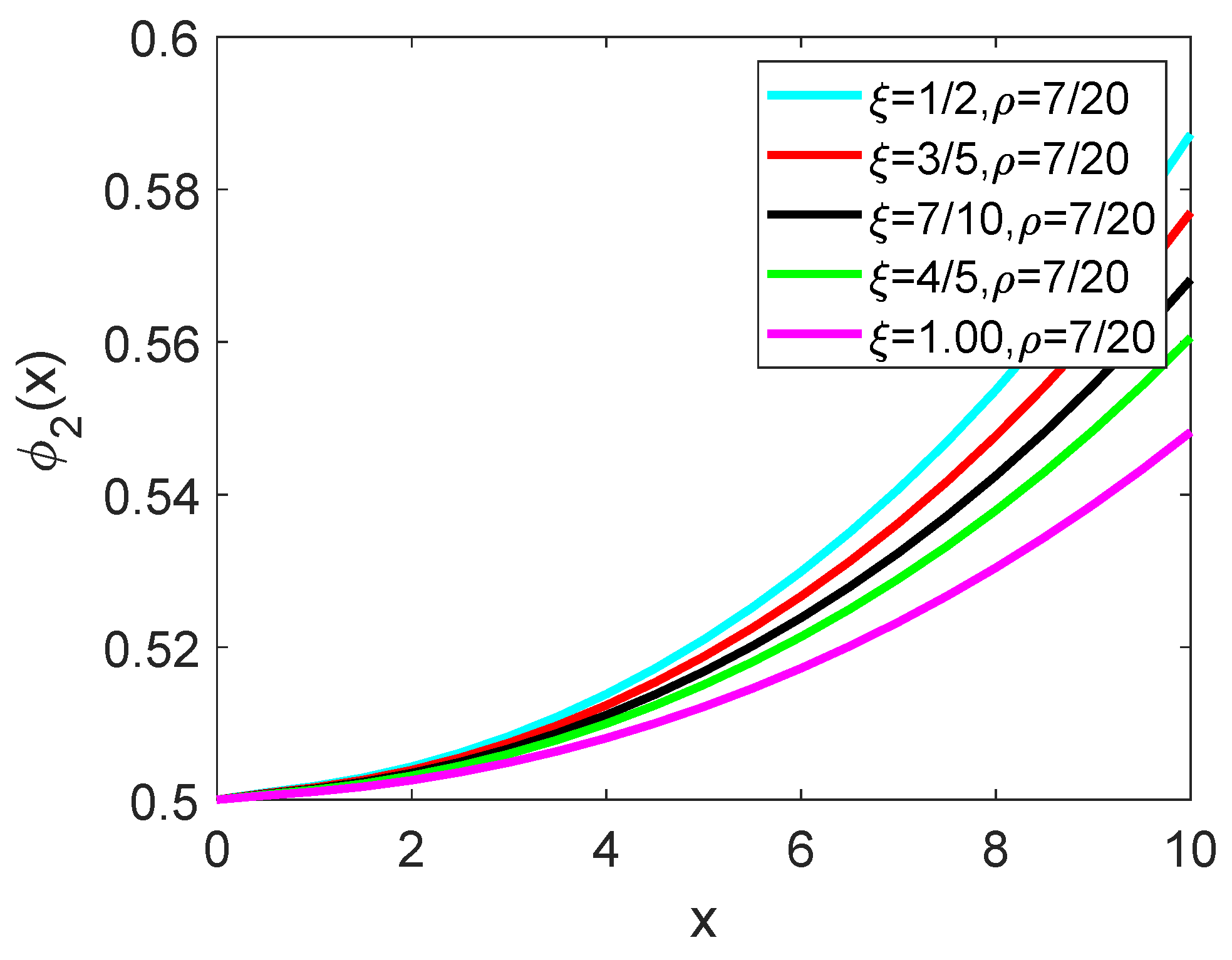
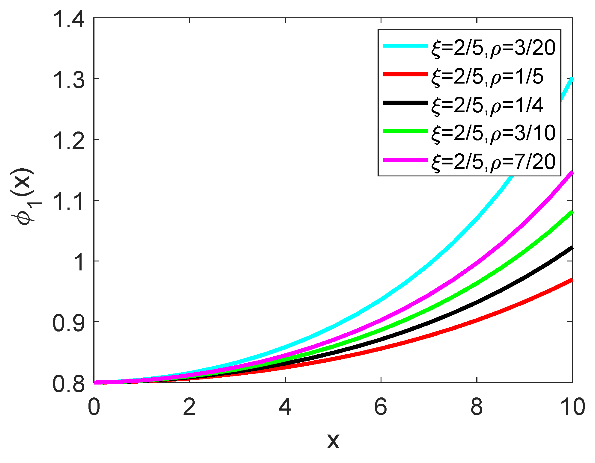
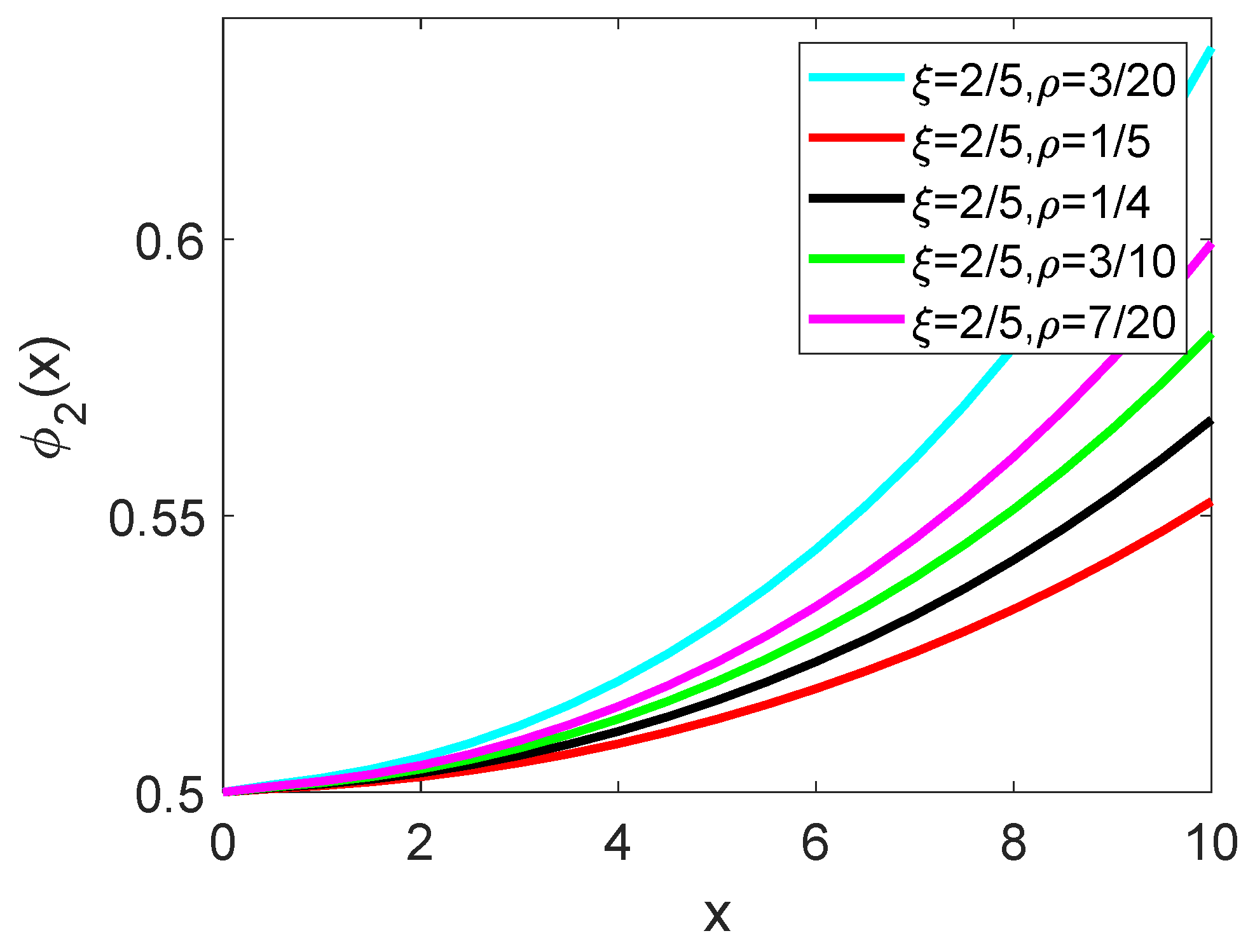
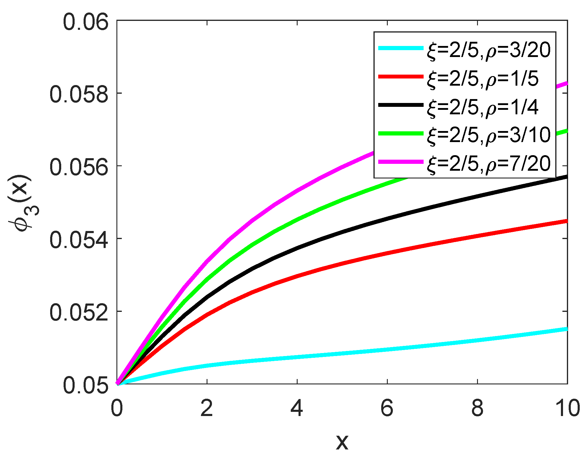
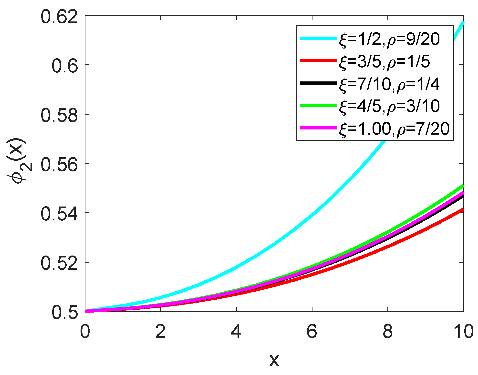
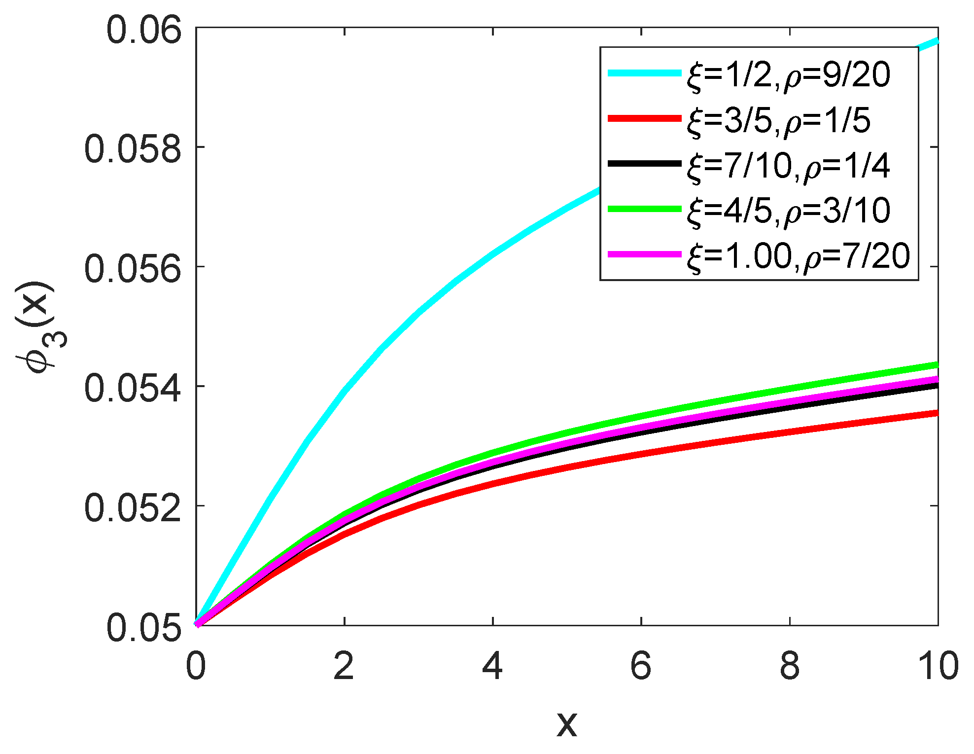
In Figure 1, Figure 2 and Figure 3, the solution is graphically represented for various fractional orders , with a fixed fractal dimension of . In Figure 4, Figure 5 and Figure 6, the solution is graphically represented with a fixed fractional order of and various fractal dimensions todemonstrate the impact of the fractal dimension. In Figure 7, Figure 8 and Figure 9, the solution is graphically represented for various fractional orders and various fractal dimensions. We observe that as the fractional order increases, the behavior of changes significantly. Higher values of lead to smoother variations, while lower values introduce more fluctuations. The system stabilizes faster for higher values of , showing reduced oscillations. In Figure 4, Figure 5 and Figure 6, we observe that changing fractal dimension affects the rate of change in . The lower values cause sharper changes, whereas higher values result in more gradual variations. The fractal nature introduces complexity in how the system evolves over time.
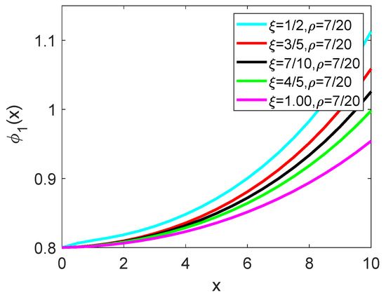
Figure 1.
Graphical representation of solution in Example 1, for various values of fractional order with same fractal value.
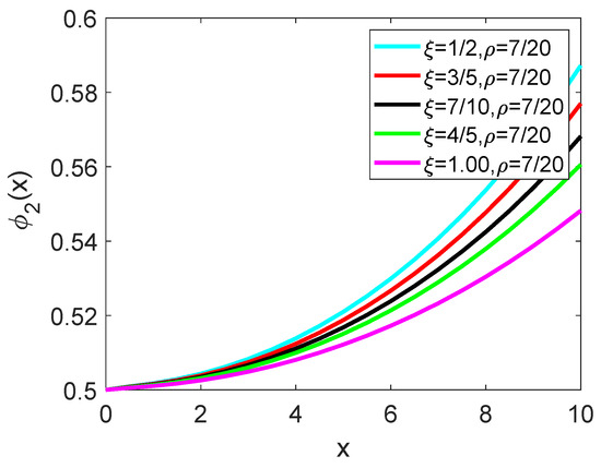
Figure 2.
Graphical representation of solution in Example 1, for various values of fractional order with same fractal value.
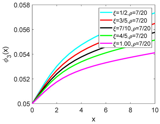
Figure 3.
Graphical representation of solution in Example 1, for various values of fractional order with same fractal value.
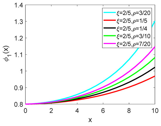
Figure 4.
Graphical representation of solution in Example 1, with same fractional orders and various fractal dimensions.
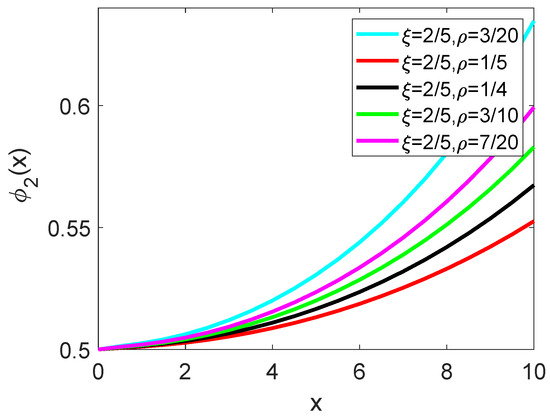
Figure 5.
Graphical representation of solution in Example 1, with same fractional orders and various fractal dimensions.
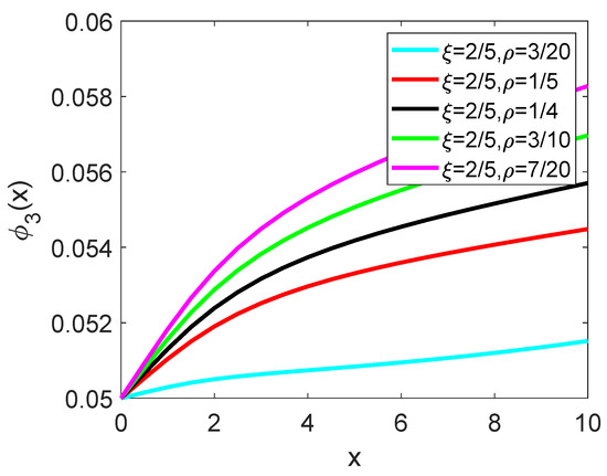
Figure 6.
Graphical representation of solution in Example 1, with same fractional orders and various fractal dimensions.
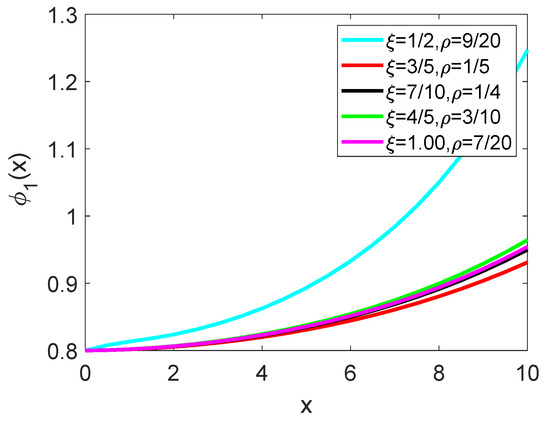
Figure 7.
Graphical representation of solution in Example 1, for various fractional orders and various fractal dimensions.
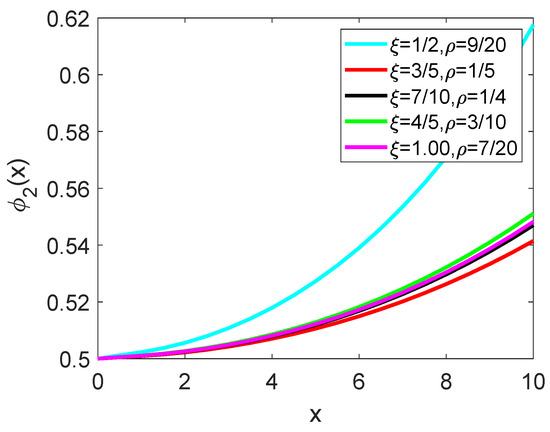
Figure 8.
Graphical representation of solution in Example 1, for various fractional orders and various fractal dimensions.
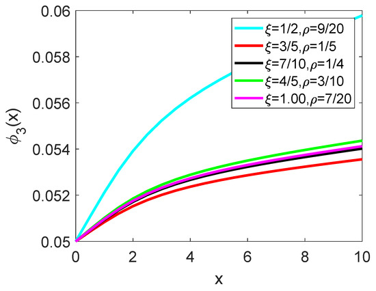
Figure 9.
Graphical representation of solution in Example 1, for various fractional orders and various fractal dimensions.
We concluded that the fractional order mainly influences the smoothness and stability of the system, while fractal dimension controls the rate and manner of change.
6. Conclusions
We have investigated a three-dimensional system of fractal-fractional-order evolution differential equations with terminal boundary conditions. We have derived sufficient criteria for the existence of solutions and for the stability of the proposed problem. The main results are applied to a general fractal-fractional-order evolution problem, and its existence and stability are verified using the main outcomes. The influence of the varying fractional order and fractal dimension on the dynamical system is analyzed through the plots of solution for various values of the fractional order and fractal dimensions . We concluded that the fractional order mainly influences the smoothness and stability of the system, while fractal dimension controls the rate and manner of change.
Solving fractal-fractional-order evolution differential equations can provide accurate predictions of the behavior of complex systems, which can be crucial in fields like physics, engineering, and finance. Fractal-fractional Caputo differential equations can model complex systems that exhibit both fractal and fractional properties, such as anomalous diffusion, chaos, and self-similarity. The power law term allows for the modeling of systems with power law behavior, which is common in natural phenomena, such as financial markets, earthquakes, and floods. These equations can capture non-local effects, which are important in systems with long-range interactions or memory. Such equations can also be used to model a wide range of systems, from physical and biological systems to financial and social systems. Solving these equations can lead to the development of new mathematical tools and techniques, which can have far-reaching implications for mathematics and science. Besides the mentioned benefits, these equations have some limitations as well. Due to their complex nature, these equations can be challenging to analyze and solve. Numerical methods for solving fractal-fractional Caputo differential equations can be computationally intensive and may require specialized algorithms. The parameters in fractal-fractional Caputo differential equations can be difficult to interpret physically, which can make it challenging to estimate them from experimental data.
Overall, fractal-fractional Caputo differential equations with a power law offer a powerful tool for modeling complex systems, but they also present significant mathematical and computational challenges.
The conclusions drawn in this article are applicable to various real-world problems where terminal conditions play a crucial role. Specifically, fractal-fractional TVPs can be useful in biological and epidemiological models, where final-state constraints are imposed.
Author Contributions
Conceptualization, F.G.; formal analysis, F.G. and R.H.E.; funding acquisition, O.O. and B.Y.; investigation, F.G., R.H.E. and O.O.; methodology, R.H.E.; project administration, K.A.; software, A.T.; writing—original draft, A.A.; and writing—review and editing, F.G., K.A. and B.Y. All authors have read and agreed to the published version of the manuscript.
Funding
This research received no external funding.
Data Availability Statement
All data are included in the paper.
Acknowledgments
The researchers would like to thank the Deanship of Graduate Studies and Scientific Research at Qassim University for financial support (QU-APC-2025).
Conflicts of Interest
The authors declare no conflicts of interest.
References
- Podlubny, I. Fractional Differential Equations; Academic Press: San Diego, CA, USA, 1999. [Google Scholar]
- Samko, S.G.; Kilbas, A.A.; Marichev, O.I. Fractional Integrals and Derivatives: Theory and Applications; Gordon and Breach: North Holland, The Netherlands, 1993. [Google Scholar]
- Alazopoulos, K.A. Non-local continuum mechanics and fractional calculus. Mech. Res. Commun. 2006, 33, 753–757. [Google Scholar] [CrossRef]
- Carpinteri, A.; Cornetti, P.; Sapora, A. A fractional calculus approach to nonlocal elasticity. Eur. Phys. J. Spec. Top. 2011, 193, 193. [Google Scholar] [CrossRef]
- Baleanu, D.; Karaca, Y.; Vázquez, L.; Macías-Díaz, J.E. Advanced fractional calculus, differential equations and neural networks: Analysis, modeling and numerical computations. Phys. Scr. 2023, 98, 110201. [Google Scholar] [CrossRef]
- Rossikhin, Y.A.; Shitikova, M.V. Application of fractional calculus for dynamic problems of solid mechanics: Novel trends and recent results. Appl. Mech. Rev. 2010, 63, 010801. [Google Scholar] [CrossRef]
- Yang, X.J. Advanced Local Fractional Calculus and Its Applications; World Science: New York, NY, USA, 2012. [Google Scholar]
- Fan, J.; He, J. Fractal derivative model for air permeability in hierarchic porous media. Abstr. Appl. Anal. 2012, 2012, 354701. [Google Scholar] [CrossRef]
- Akgül, A. Analysis and new applications of fractal fractional differential equations with power law kernel. Discret. Contin. Dyn. Syst. S 2021, 14, 3401–3417. [Google Scholar] [CrossRef]
- Karaca, Y.; Baleanu, D. A novel R/S fractal analysis and wavelet entropy characterization approach for robust forecasting based on self-similar time series modeling. Fractals 2020, 28, 2040032. [Google Scholar] [CrossRef]
- Hamza, A.; Osman, O.; Ali, A.; Alsulami, A.; Aldwoah, K.; Mustafa, A.; Saber, H. Fractal-Fractional-Order Modeling of Liver Fibrosis Disease and Its Mathematical Results with Subinterval Transitions. Fractal Fract. 2024, 8, 638. [Google Scholar] [CrossRef]
- Karaca, Y.; Moonis, M.; Baleanu, D. Fractal and multifractional-based predictive optimization model for stroke subtypes’ classification. Chaos Solitons Fractals 2020, 136, 109820. [Google Scholar] [CrossRef]
- Alraqad, T.; Almalahi, M.A.; Mohammed, N.; Alahmade, A.; Aldwoah, K.A.; Saber, H. Modeling Ebola Dynamics with a Piecewise Hybrid Fractional Derivative Approach. Fractal Fract. 2024, 8, 596. [Google Scholar] [CrossRef]
- File, G.; Reddy, Y.N. Terminal boundary-value technique for solving singularly perturbed delay differential equations. J. Taibah Univ. Sci. 2014, 8, 289–300. [Google Scholar] [CrossRef]
- Palamides, A.P.; Yannopoulos, T.G. Terminal value problem for singular ordinary differential equations: Theoretical analysis and numerical simulations of ground states. Bound. Value Probl. 2006, 2006, 28719. [Google Scholar] [CrossRef]
- Shreve, W.E. Terminal value problems for second order nonlinear differential equations. SIAM J. Appl. Math. 1970, 18, 783–791. [Google Scholar] [CrossRef]
- Aftabizadeh, A.R.; Lakshmikantham, V. On the theory of terminal value problems for ordinary differential equations. Nonlinear Anal. Theory Methods Appl. 1981, 5, 1173–1180. [Google Scholar] [CrossRef]
- Diethelm, K. An extension of the well-posedness concept for fractional differential equations of Caputo’s type. Appl. Anal. 2014, 93, 2126–2135. [Google Scholar] [CrossRef]
- Shiri, B.; Wu, G.C.; Baleanu, D. Terminal value problems for nonlinear systems of fractional differential equations. Appl. Numer. Math. 2021, 170, 162–178. [Google Scholar] [CrossRef]
- Ford, N.J.; Morgado, M.L.; Rebelo, M. High order numerical methods for fractional terminal value problems. Comput. Methods Appl. Math. 2014, 14, 55–70. [Google Scholar] [CrossRef]
- Boichuk, O.; Feruk, V. Terminal value problem for the system of fractional differential equations with additional restrictions. Math. Model. Anal. 2025, 30, 120–141. [Google Scholar] [CrossRef]
- Bao, N.T.; Caraballo, T.; Tuan, N.H.; Zhou, Y. Existence and regularity results for terminal value problem for nonlinear fractional wave equations. Nonlinearity 2021, 34, 1448. [Google Scholar] [CrossRef]
- Assanova, A.T.; Uteshova, R.E. A singular boundary value problem for evolution equations of hyperbolic type. Chaos Solitons Fractals 2021, 143, 110517. [Google Scholar] [CrossRef]
- Racke, R. Lectures on Nonlinear Evolution Equations: Initial Value Problems; Birkhäuser: Basel, Switzerland, 2015. [Google Scholar]
- Atangana, A. Fractal-fractional differentiation and integration: Connecting fractal calculus and fractional calculus to predict complex systems. Chaos Solitons Fractals 2017, 102, 396–406. [Google Scholar] [CrossRef]
- Shah, K.; Abdeljawad, T. Study of radioactive decay process of uranium atoms via fractals-fractional analysis. S. Afr. J. Chem. Eng. 2024, 48, 63–70. [Google Scholar] [CrossRef]
- Khan, H.; Aslam, M.; Rajpar, A.H.; Chu, Y.M.; Etemad, S.; Rezapour, S.; Ahmad, H. A new fractal-fractional hybrid model for studying climate change on coastal ecosystems. Fractals 2024, 32, 2440015. [Google Scholar] [CrossRef]
- Khan, H.; Alzabut, J.; Shah, A.; He, Z.Y.; Etemad, S.; Rezapour, S.; Zada, A. On fractal-fractional waterborne disease model: A study on theoretical and numerical aspects via simulations. Fractals 2023, 31, 2340055. [Google Scholar] [CrossRef]
- Shah, A.; Khan, H.; De la Sen, M.; Alzabut, J.; Etemad, S.; Deressa, C.T.; Rezapour, S. On non-symmetric fractal-fractional modeling for ice smoking. Symmetry 2022, 15, 87. [Google Scholar] [CrossRef]
- Madani, Y.A.; Rabih, M.N.A.; Alqarni, F.A.; Ali, Z.; Aldwoah, K.A.; Hleili, M. Existence, Uniqueness, and Stability of a Nonlinear Tripled Fractional Order Differential System. Fractal Fract. 2024, 8, 416. [Google Scholar] [CrossRef]
- Algolam, M.S.; Osman, O.; Ali, A.; Mustafa, A.; Aldwoah, K.; Alsulami, A. Fixed Point and Stability Analysis of a Tripled System of Nonlinear Fractional Differential Equations with n-Nonlinear Terms. Fractal Fract. 2024, 8, 697. [Google Scholar] [CrossRef]
- Bainov, D.D.; Simenonv, P.S. Impulsive Differential Equations: Periodic Solutions and Applications; Longman: Harlow, UK, 1993. [Google Scholar]
- Ali, A.; Rabiei, F.; Shah, K. On Ulam’s Type Stability for a Class of Impulsive Fractional Differential Equations with Nonlinear Integral Boundary Conditions. J. Nonlinear Sci. Appl. 2017, 10, 4760–4775. [Google Scholar] [CrossRef]
- Pietsch, A. History of Banach Spaces and Linear Operators; Springer Science & Business Media: Cham, Switzerland, 2007. [Google Scholar]
- Granas, A.; Dugundji, J. Fixed Point Theory; Springer: New York, NY, USA, 2003. [Google Scholar]
- Schaefer, H. Über die Methode der a Priori-Schranken. Math. Ann. 1955, 129, 415–416. [Google Scholar] [CrossRef]
- Rus, I.A. Ulam Stabilities of Ordinary Differential Equations in a Banach Space. Carpath. J. Math. 2010, 26, 103–107. [Google Scholar]


Disclaimer/Publisher’s Note: The statements, opinions and data contained in all publications are solely those of the individual author(s) and contributor(s) and not of MDPI and/or the editor(s). MDPI and/or the editor(s) disclaim responsibility for any injury to people or property resulting from any ideas, methods, instructions or products referred to in the content. |
© 2025 by the authors. Licensee MDPI, Basel, Switzerland. This article is an open access article distributed under the terms and conditions of the Creative Commons Attribution (CC BY) license (https://creativecommons.org/licenses/by/4.0/).