Fractal Sturm–Liouville Theory

Abstract

This paper provides a short summary of fractal calculus and its application to generalized Sturm–Liouville theory. It presents both the fractal homogeneous and non-homogeneous Sturm–Liouville problems and explores the theory’s applications in optics. We include examples and graphs to illustrate the effect of fractal support on the solutions and propose new models for fractal structures.

1. Introduction

Fractals, characterized by their non-integer dimensions, represent a departure from traditional geometric shapes [1,2]. Unlike linear paths, perfect spheres, or cone-like structures found in classical geometry, natural phenomena such as lightning, clouds, and mountains exhibit intricate shapes that defy conventional mathematical description [3]. Consequently, the study of fractal geometry has become essential for capturing the complexity of these natural forms [3].

Research efforts have focused on identifying and analyzing fractal patterns emerging from various processes, including social phenomena [4]. Techniques such as box-counting have been instrumental in quantifying the spatial and temporal attributes of fractal patterns across diverse contexts, ranging from Saturn’s rings to brain imaging data [5]. Moreover, analytical applications of Iterated Function Systems (IFS) methods have showcased their utility in modeling complex systems inspired by fractal frameworks [6].

The integration of fractal and fractal-rate point processes has provided a rigorous yet practical approach to analyze and model complex systems [7]. This synthesis combines the scaling properties of fractals with the discrete nature of random point processes, offering insights into diverse fields such as polymer synthesis and environmental engineering [7,8,9]. Fractal analysis has found applications in various scientific domains, including genetics, medicine, ecology, and physics [10,11,12,13]. Techniques such as fractal dimension analysis have been instrumental in understanding complex biological phenomena, ecological systems, and physical processes [11,12,13].

In response to the challenges posed by fractal phenomena, researchers have explored advanced mathematical methods such as fractional calculus [14], harmonic analysis [15], and measure theory [16,17,18,19]. These methods have been instrumental in developing numerical techniques for solving partial differential equations on fractals [20]. While traditional calculus remains applicable in many scenarios, fractal calculus offers a tailored mathematical framework for handling equations with fractal solutions [21,22]. Its elegant and algorithmic approaches have rendered it particularly attractive for modeling fractal phenomena [23,24].

The gauge integral approach has proven effective in extending $F^{\alpha }$-calculus (FC), particularly in integrating functions over designated subsets [23] of the real number line. This extension accommodates singularities inherent to fractal sets. Fractal differential equations have been formulated for various circuit configurations subject to zero-mean additive white Gaussian noise, incorporating a fractal time element [25,26,27]. It was proposed that two separate del-operators could be defined in spaces with non-integer dimensions, each operating on a vector field and a scalar field, respectively. These del-operators were subsequently employed to establish the conventional expressions for the Laplacian and fundamental vector differential operators in spaces with fractional dimensions [28]. The study investigated methods analogous to the separable method and integrating factor methodology for solving $\alpha$-order differential equations [29]. The study also established a connection between the conventional Fokker–Planck Equation and its fractal version, incorporating fractal derivatives [30]. A fractal discharging model for batteries was devised to explore the influence of non-locality on solution behavior and elucidate how the system’s prior state affects its present state [23]. The research showcased the efficacy of non-local fractal derivatives in characterizing fractional Brownian motion on thin Cantor-like sets. Additionally, it introduced a staircase function linked to a fractal comb, which served as a tool for defining derivatives and integrals for functions defined on these combs [31].

The formulation of fuzzy fractal calculus involves articulating the concepts of fractal limit, continuity, derivative, and integral within the realm of fuzzy mathematics [32]. Solutions to fractal differential equations have been derived, accompanied by the establishment of their stability conditions [23]. The fractal Einstein field equations were introduced, underscoring their relevance and practical applicability on fractal manifolds [33]. The Laplace transform and local Fourier transform concepts have been extended to fractal curves, enabling the solution of fractal differential equations with constant coefficients [23,34].

Numerical methods play a crucial role in finding approximate solutions to ordinary differential equations (ODEs) when exact solutions are either unavailable or impractical to compute [35]. While some ODEs have analytical solutions, many real-world problems involve complex equations for which analytical solutions are not feasible. In such cases, numerical approximation methods provide practical tools for engineers and scientists to obtain solutions that meet their accuracy requirements. This paper investigates numerical methods for solving fractal differential equations, building upon the foundation laid by previous research in fractal calculus and mathematical modeling [36].

The algorithms and techniques discussed in this paper are designed to compute numerical approximations to the solutions of the fractal differential equations [35]. The outlines of numerical methods for solving partial differential equations on fractals are also provided. This covers both strong and weak forms of the equations, using standard graph Laplacian matrices and discrete approximations of fractal sets [20].

The self-adjointness of the differential operator generated by the $F^{\alpha }$-derivative has been proven [37]. The fractal Sturm–Liouville problem is formulated using a new calculus defined on fractal subsets of real numbers. The existence and uniqueness theorem for such equations has been proven [38].

Hofstadter’s butterfly has been challenging to observe due to extreme experimental conditions. High-resolution scanning tunneling microscopy/spectroscopy (STM/STS) has been used to investigate twisted bilayer graphene near the second magic angle, where the fractionalization of moiré bands into Hofstadter subbands has been revealed, and experimental signatures of self-similarity have been discerned. A dynamically evolving spectrum has been uncovered, influenced by strong correlations, Coulomb interactions, and electron quantum degeneracy, extending beyond Hofstadter’s original model [39].

In this paper, we continue these studies and present applications in optics.

The outline of this paper is as follows:

In Section 2, we review fractal calculus. In Section 3, we present the generalized Sturm–Liouville theory, addressing both the fractal homogeneous and non-homogeneous Sturm–Liouville problems. In Section 4, we explore applications of the generalized Sturm–Liouville theory in optics. Finally, in Section 5, we provide the conclusion.

2. Fractal Calculus Review

This section provides an overview of fractal calculus. For more details, refer to [21,22,23].

Definition 1.

The flag function $\upsilon (F,I)$ for a set $F\subset \mathbb{R}$ and interval $I=[a,b]$ is as follows:

$$\upsilon (F,I)=\left\{\begin{array}{cc}1,\hfill & \mathrm{if}F\cap I\ne \varnothing ;\hfill \\ 0,\hfill & \mathit{otherwise}.\hfill \end{array}\right.$$

Definition 2.

For a subdivision $P_{[a,b]}=\{t_0=a,\dots ,t_n=b\}$ of $[a,b]$ and $\delta >0$, the coarse mass of F is:

$${\tau }_{\delta }^{\alpha }(F,a,b)={\displaystyle \underset{|P|\le \delta }{\inf }}{\displaystyle \sum _{i=0}^{n-1}}\Gamma (\alpha +1){(t_{i+1}-t_i)}^{\alpha }\upsilon (F,[t_i,t_{i+1}]),$$

where $|P|={\max }_{0\le i\le n-1}(t_{i+1}-t_i)$, and $0<\alpha \le 1$.

Definition 3.

The mass function of F is the limit as $\delta \to 0$:

$${\tau }^{\alpha }(F,a,b)={\displaystyle \underset{\delta \to 0}{\lim }}{\tau }_{\delta }^{\alpha }(F,a,b).$$

Definition 4.

The τ-dimension of $F\cap [a,b]$ is defined as follows:

$$\begin{array}{cc}\hfill {\dim }_{\tau }(F\cap [a,b])& =\inf \{\alpha :{\tau }^{\alpha }(F,a,b)=0\}\hfill \\ & =\sup \{\alpha :{\tau }^{\alpha }(F,a,b)=\infty \}.\hfill \end{array}$$

Definition 5.

The integral staircase function of F is defined as follows:

$$S_F^{\alpha }\left(x\right)=\left\{\begin{array}{cc}{\tau }^{\alpha }(F,a_0,x),\hfill & \mathit{if}x\ge a_0;\hfill \\ -{\tau }^{\alpha }(F,x,a_0),\hfill & \mathit{otherwise}.\hfill \end{array}\right.$$

Definition 6.

A function $q:F\to \mathbb{R}$ is F-continuous at x if:

$$q\left(x\right)={\displaystyle \underset{y\to x}{F_{-}\mathit{lim}}}q\left(y\right).$$

Definition 7.

The $F^{\alpha }$-derivative of a function q at $x\in F$ is as follows:

$$D_F^{\alpha }q\left(x\right)={\displaystyle \underset{y\to x}{F_{-}\mathit{lim}}}{\displaystyle \frac{q\left(y\right)-q\left(x\right)}{S_F^{\alpha }\left(y\right)-S_F^{\alpha }\left(x\right)}}.$$

Definition 8.

The $F^{\alpha }$-integral of a function q on $F\subset \mathbb{R}$ is as follows:

$${\int }_a^{b}q\left(x\right)d_F^{\alpha }x={\displaystyle \underset{P_{[a,b]}}{\sup }}{\displaystyle \sum _{i=0}^{n-1}}{\displaystyle \underset{x\in F\cap I}{\inf }}q\left(x\right)(S_F^{\alpha }\left(x_{i+1}\right)-S_F^{\alpha }\left(x_i\right)).$$

where $P_{[a,b]}=\{t_0=a,\dots ,t_n=b\}$ of $[a,b]$.

3. Generalized Sturm–Liouville Theory

Sturm–Liouville theory [40,41], a basic framework in differential equations and mathematical physics that deals with a class of second-order linear differential equations [42,43], is presented here in a generalized version. In particular, we present the Sturm–Liouville problems that are fractal homogeneous and fractal non-homogeneous.

3.1. The Fractal Homogeneous Sturm–Liouville Problem

We begin by formulating the fractal homogeneous Sturm–Liouville problem. The classical second-order linear differential equation has been extensively studied using Sturm–Liouville theory [44,45]. Here, we extend this framework to the second $\alpha$-order linear differential equation, given as follows:

$$D_F^{\alpha }\left[p\left(x\right)D_F^{\alpha }y\right]+\left[\lambda w\left(x\right)-q\left(x\right)\right]y=0,x\in F,$$

(1)

where $y\left(x\right)$ is the unknown fractal function (fractal eigenfunction), and $\lambda$ is a parameter (fractal eigenvalue). The functions $p\left(x\right):F\to \mathbb{R}$, $q\left(x\right):F\to \mathbb{R}$, and $w\left(x\right):F\to \mathbb{R}$ are F-continuous, with $p\left(x\right)>0$ and $w\left(x\right)>0$.

Remark 1.

We note that F represents a fractal set, such as the Cantor set, and α denotes its fractal dimension, as defined in Definition 4.

The fractal differential operator is defined as follows:

$$L_F\left[y\right]=-D_F^{\alpha }\left[p\left(x\right)D_F^{\alpha }y\right]+q\left(x\right)y.$$

(2)

where $y:F\to \mathbb{R}$ belongs to the space of $F^{\alpha }$-differentiable functions. This fractal operator is fractal self-adjoint with respect to the fractal weight function $w\left(x\right)$ if it satisfies the following condition:

$${\int }_a^{b}u\left(x\right)L_F\left[v\left(x\right)\right]d_F^{\alpha }x={\int }_a^{b}v\left(x\right)L_F\left[u\left(x\right)\right]d_F^{\alpha }x,$$

(3)

for suitable functions $u\left(x\right)$ and $v\left(x\right)$, provided that the boundary terms vanish. To verify the fractal self-adjoint property, we perform fractal integration by parts:

$${\int }_a^{b}u\left[-D_F^{\alpha }\left(p{D}_F^{\alpha }v\right)+qv\right]d_F^{\alpha }x={\int }_a^{b}v\left[-D_F^{\alpha }\left(p{D}_F^{\alpha }u\right)+qu\right]d_F^{\alpha }x,$$

(4)

after simplifying and using the following condition:

$${\left[up{D}_F^{\alpha }v-vp{D}_F^{\alpha }u\right]}_a^b=0,$$

(5)

which holds if appropriate fractal boundary conditions are satisfied [46,47,48]:

• Dirichlet: $u\left(x\right){|}_{x=S_F^{\alpha }\left(a\right)}=u\left(x\right){|}_{x=S_F^{\alpha }\left(b\right)}=0$.
• Neumann: $D_F^{\alpha }u\left(x\right){|}_{x=S_F^{\alpha }\left(a\right)}=D_F^{\alpha }u\left(x\right){|}_{x=S_F^{\alpha }\left(b\right)}=0$.
• Robin:

  $$\begin{array}{cc}\hfill & a_{1}u\left(x\right){|}_{x=S_F^{\alpha }\left(a\right)}+b_1{D}_F^{\alpha }u\left(x\right){|}_{x=S_F^{\alpha }\left(a\right)}=0,\hfill \\ \hfill & a_{2}u\left(x\right){|}_{x=S_F^{\alpha }\left(b\right)}+b_2{D}_F^{\alpha }u\left(x\right){|}_{x=S_F^{\alpha }\left(b\right)}=0.\hfill \end{array}$$

  (6)

Under these conditions, $L_F$ is fractal self-adjoint in the fractal space $L_w^2\left(F\right)$ [21,22,23].

Remark 2.

We observe that by utilizing Equations (5) and (6), we can rewrite the expression as follows:

$$\begin{array}{cc}& {\left[u\left(x\right)p\left(x\right)D_F^{\alpha }v\left(x\right)\right]}_a^b-{\left[v\left(x\right)p\left(x\right)D_F^{\alpha }u\left(x\right)\right]}_a^b\hfill \\ & =p\left(b\right)\left(u\left(b\right)D_F^{\alpha }v\left(b\right)-v\left(b\right)D_F^{\alpha }u\left(b\right)\right)-p\left(a\right)\left(u\left(a\right)D_F^{\alpha }v\left(a\right)-v\left(a\right)D_F^{\alpha }u\left(a\right)\right)\hfill \\ & =p\left(b\right)\left(u\left(b\right)\left(-{\displaystyle \frac{a_2}{b_2}}v\left(b\right)\right)-v\left(b\right)\left(-{\displaystyle \frac{a_2}{b_2}}u\left(b\right)\right)\right)\hfill \\ & -p\left(a\right)\left(u\left(a\right)\left(-{\displaystyle \frac{a_1}{b_1}}v\left(a\right)\right)-v\left(a\right)\left(-{\displaystyle \frac{a_1}{b_1}}u\left(a\right)\right)\right)\hfill \\ & =p\left(b\right)\left(-{\displaystyle \frac{a_2}{b_2}}u\left(b\right)v\left(b\right)+{\displaystyle \frac{a_2}{b_2}}v\left(b\right)u\left(b\right)\right)-p\left(a\right)\left(-{\displaystyle \frac{a_1}{b_1}}u\left(a\right)v\left(a\right)+{\displaystyle \frac{a_1}{b_1}}v\left(a\right)u\left(a\right)\right)\hfill \\ & =0.\hfill \end{array}$$

Thus, the fractal Robin boundary conditions are satisfied.

Definition 9.

Let $\mathit{Sch}\left(h\right)$ be an α-perfect set, and define the weighted fractal Hilbert space as follows [23]:

$$L_{2,w}^{\alpha }(0,1)=\left\{h:{\int }_0^1{\left|h\left(x\right)\right|}^{2}w\left(x\right)d_F^{\alpha }x<\infty \right\}.$$

(7)

This space is equipped with the inner product [23]:

$$(h,g)={\int }_0^{1}h\left(x\right)g\left(x\right)w\left(x\right)d_F^{\alpha }x.$$

(8)

The $F^{\alpha }$-Wronskian of functions h and g is given as follows:

$$W^{\alpha }\left(x\right)=h\left(x\right)D_F^{\alpha }g\left(x\right)-g\left(x\right)D_F^{\alpha }h\left(x\right),x\in [0,1].$$

(9)

Definition 10.

Let $u(x,\lambda )$ and $v(x,\lambda )$ be solutions to the following equation:

$$-D_F^{\alpha }\left[p\left(x\right)D_F^{\alpha }y\right]+q\left(x\right)y=\lambda w\left(x\right)y,$$

(10)

satisfying the following boundary conditions:

$$\begin{array}{cc}\hfill u(0,\lambda )& =-a_2,D_F^{\alpha }u(0,\lambda )=a_1,\hfill \end{array}$$

(11)

$$\begin{array}{cc}\hfill v(1,\lambda )& =-b_2,D_F^{\alpha }v(1,\lambda )=b_1.\hfill \end{array}$$

(12)

It follows that

$$\Delta \left(\lambda \right)=W^{\alpha }(u,v)\ne 0.$$

(13)

Thus, the Green’s function is defined as follows:

$$G(x,y,\lambda )=-{\displaystyle \frac{1}{\Delta \left(\lambda \right)}}\left\{\begin{array}{cc}v(x,\lambda )u(y,\lambda ),\hfill & 0\le y\le x\le 1,\hfill \\ u(x,\lambda )v(y,\lambda ),\hfill & 0\le x\le y\le 1.\hfill \end{array}\right.$$

(14)

Theorem 1

([49]). Let A be the operator, defined as follows:

$$A{x}_i=y_i,$$

(15)

where

$$y_i={\displaystyle \sum _{k=1}^{\infty }}{a}_{ik}{x}_k,i,k\in \mathbb{N}.$$

(16)

If

$${\displaystyle \sum _{i,k=1}^{\infty }}{|a_{ik}|}^2<+\infty ,$$

(17)

then A is a compact operator in $l^2$, where $l^2$ is the standard sequence space.

Definition 11.

Assuming without loss of generality that $\lambda =0$ is not an eigenvalue, we define the following:

$$G(x,y):=G(x,y,0),$$

(18)

which simplifies to the following:

$$G\left(x,y\right):=G\left(x,y,0\right)$$

(19)

$$G(x,y,\lambda )=-{\displaystyle \frac{1}{\Delta \left(\lambda \right)}}\left\{\begin{array}{cc}v\left(x\right)u\left(y\right),\hfill & 0\le y\le x\le 1,\hfill \\ u\left(x\right)v\left(y\right),\hfill & 0\le x\le y\le 1.\hfill \end{array}\right.$$

(20)

Theorem 2.

The function $G(x,y)$ defined by Equation (20) is a fractal Hilbert–Schmidt kernel.

Proof. 

Based on the definition of $G(x,y)$, we have the following:

$${\int }_0^1{d}_F^{\alpha }x{\int }_0^x{|G(x,y)|}^{2}w\left(y\right)d_F^{\alpha }y<+\infty ,$$

(21)

and

$${\int }_0^1{d}_F^{\alpha }x{\int }_x^1{|G(x,y)|}^{2}w\left(y\right)d_F^{\alpha }y<+\infty .$$

(22)

Since the inner integral exists and $v\left(x\right)u\left(y\right)\in L_{2,w}^{\alpha }(0,1)\times L_{2,w}^{\alpha }(0,1)$, it follows that:

$${\int }_0^1{\int }_0^1{|G(x,y)|}^{2}w\left(y\right)d_F^{\alpha }x{d}_F^{\alpha }y<+\infty .$$

(23)

□

Theorem 3.

Let $L_F^{-1}$ be the operator, defined as follows:

$$\left(L_F^{-1}g\right)\left(t\right)={\int }_0^{1}G(x,y)f\left(y\right)w\left(y\right)d_F^{\alpha }y.$$

(24)

Then, $L_F^{-1}$ is a compact operator.

Proof. 

Let ${\varphi }_i$ where $i\in \mathbb{N}$ be a complete orthonormal basis of $L_{2,w}^{\alpha }(0,1)$. We define the following:

$$\begin{array}{cc}\hfill x_i& =(f,{\varphi }_i)={\int }_0^{1}f\left(x\right){\varphi }_i\left(x\right)w\left(x\right)d_F^{\alpha }x,\hfill \end{array}$$

(25)

$$\begin{array}{cc}\hfill y_i& =(g,{\varphi }_i)={\int }_0^{1}g\left(x\right){\varphi }_i\left(x\right)w\left(x\right)d_F^{\alpha }x,\hfill \end{array}$$

(26)

$$\begin{array}{cc}\hfill a_{ik}& ={\int }_0^1{\int }_0^{1}G(x,y)\overline{{\varphi }_i^{\left(1\right)}\left(x\right)}\overline{{\varphi }_k^{\left(1\right)}\left(y\right)}w\left(x\right)d_F^{\alpha }x{d}_F^{\alpha }y.\hfill \end{array}$$

(27)

Since $L_{2,w}^{\alpha }(0,1)$ is isometrically mapped onto $l^2$, the operator $L_F^{-1}$ corresponds to the operator A in $l^2$. The condition on $G(x,y)$ ensures that:

$${\displaystyle \sum _{i,k=1}^{\infty }}{|a_{ik}|}^2<+\infty ,$$

(28)

which, based on Theorem 1, implies that both A and $L_F^{-1}$ are compact operators. □

Theorem 4.

Fractal self-adjointness ensures the existence of an infinite sequence of real fractal eigenvalues ${\lambda }_n^{\alpha }$ that can be ordered as follows:

$${\lambda }_1^{\alpha }<{\lambda }_2^{\alpha }<{\lambda }_3^{\alpha }<\dots$$

Moreover, the corresponding fractal eigenfunctions are mutually orthogonal with respect to the fractal weight function.

Proof. 

To prove this theorem, consider the fractal eigenvalue problem:

$$L_F\left[y_n\right]={\lambda }_n^{\alpha }w\left(x\right)y_n,$$

where $L_F$ is a fractal self-adjoint operator, ${\lambda }_n^{\alpha }$ are the fractal eigenvalues, and $y_n\left(x\right)$ are the corresponding fractal eigenfunctions. The fractal Rayleigh quotient gives the following:

$${\lambda }_n^{\alpha }={\displaystyle \frac{{\int }_a^b{y}_n\left(x\right)L_F\left[y_n\left(x\right)\right]w\left(x\right)d_F^{\alpha }x}{{\int }_a^b{y}_n^2\left(x\right)w\left(x\right)d_F^{\alpha }x}}.$$

By applying the minimax principle [50,51,52], we obtain the following ordering [50]:

$${\lambda }_1^{\alpha }<{\lambda }_2^{\alpha }<{\lambda }_3^{\alpha }<\cdots$$

where ${\lambda }_n^{\alpha }$ is given as follows:

$${\lambda }_n^{\alpha }={\displaystyle \underset{V_n}{\min }}{\displaystyle \underset{y\in V_n\setminus \left\{0\right\}}{\max }}{\displaystyle \frac{{\int }_a^{b}y\left(x\right)L_F\left[y\left(x\right)\right]w\left(x\right)d_F^{\alpha }x}{{\int }_a^b{y}^2\left(x\right)w\left(x\right)d_F^{\alpha }x}},$$

where $V_n$ is an $n\alpha$-dimensional subspace of the fractal function space [53]. □

Remark 3.

The solution space for higher α-order linear fractal differential equations has a dimensionality of $n\alpha$ [53].

To prove orthogonality, consider the fractal self-adjointness property:

$${\int }_a^{b}y\left(x\right)L_F\left[z\left(x\right)\right]d_F^{\alpha }x={\int }_a^{b}z\left(x\right)L_F\left[y\left(x\right)\right]d_F^{\alpha }x,$$

for any suitable fractal functions $y\left(x\right)$ and $z\left(x\right)$. Setting $y\left(x\right)=y_m\left(x\right)$ and $z\left(x\right)=y_n\left(x\right)$, we obtain the following:

$${\int }_a^b{y}_m\left(x\right)L_F\left[y_n\left(x\right)\right]d_F^{\alpha }x={\int }_a^b{y}_n\left(x\right)L_F\left[y_m\left(x\right)\right]d_F^{\alpha }x.$$

Using the eigenvalue equation, this becomes:

$${\int }_a^b{y}_m\left(x\right){\lambda }_n^{\alpha }{y}_n\left(x\right)d_F^{\alpha }x={\int }_a^b{y}_n\left(x\right){\lambda }_m^{\alpha }{y}_m\left(x\right)d_F^{\alpha }x,$$

which simplifies to:

$${\lambda }_n^{\alpha }{\int }_a^b{y}_m\left(x\right)y_n\left(x\right)d_F^{\alpha }x={\lambda }_m^{\alpha }{\int }_a^b{y}_m\left(x\right)y_n\left(x\right)d_F^{\alpha }x.$$

Rearranging yields:

$$({\lambda }_n^{\alpha }-{\lambda }_m^{\alpha }){\int }_a^b{y}_m\left(x\right)y_n\left(x\right)d_F^{\alpha }x=0.$$

Since ${\lambda }_n^{\alpha }\ne {\lambda }_m^{\alpha }$ for $m\ne n$, it follows that:

$${\int }_a^b{y}_m\left(x\right)y_n\left(x\right)d_F^{\alpha }x=0,$$

proving that the fractal eigenfunctions corresponding to distinct fractal eigenvalues are orthogonal with respect to the weight function $w\left(x\right)$. □

Theorem 5.

The set of all normalized eigenfunctions of $L_F$ forms an orthonormal basis for $L_{2,w}^{\alpha }\left(0,1\right).$ The eigenvalues of $L_F$ form an infinite sequence ${\left\{{\lambda }_i^{\alpha }\right\}}_{i=1}^{\infty }$ of real numbers such that

$$|{\lambda }_1^{\alpha }|<|{\lambda }_2^{\alpha }|<\dots <|{\lambda }_i^{\alpha }|<\dots \to \infty \mathit{as}i\to \infty .$$

(29)

Proof. 

It follows from the Hilbert–Schmidt theorem and Theorem 3 that $L_F^{-1}$ has an infinite sequence of non-zero real eigenvalues ${\left\{{\eta }_i^{\alpha }\right\}}_{i=1}^{\infty }$ with ${\eta }_i^{\alpha }\to 0$$(i\to \infty ).$ Then, we see that

$$\left|{\lambda }_i^{\alpha }\right|={\displaystyle \frac{1}{\left|{\eta }_i^{\alpha }\right|}}\to \infty \mathrm{as}i\to \infty .$$

(30)

Let ${\left\{{\psi }_i\right\}}_{i=1}^{\infty }$ be an orthonormal set of eigenfunctions corresponding to ${\left\{{\eta }_i^{\alpha }\right\}}_{i=1}^{\infty }.$ Thus, we find

$$u\in L_{2,w}^{\alpha }\left(0,1\right),L_F^{-1}u=\Xi ,L_F\Xi =u,L_F{\psi }_i={\lambda }_i^{\alpha }{\psi }_i(i\in \mathbb{N})$$

(31)

and

$$\begin{array}{cc}\hfill u& =L_F\Xi ={\displaystyle \sum _{i=1}^{\infty }}\left(u,{\psi }_i\right){\psi }_i={\displaystyle \sum _{i=1}^{\infty }}\left(L_F\Xi ,{\psi }_i\right){\psi }_i\hfill \\ & ={\displaystyle \sum _{i=1}^{\infty }}\left(\Xi ,L_F{\psi }_i\right){\psi }_i={\displaystyle \sum _{i=1}^{\infty }}{\lambda }_i^{\alpha }\left(\Xi ,{\psi }_i\right){\psi }_i.\hfill \end{array}$$

(32)

□

Example 1.

Consider the fractal Sturm–Liouville equation:

$$D_F^{\alpha }\left[(1-S_F^{\alpha }{\left(x\right)}^2)D_F^{\alpha }y\right]+\left[\lambda -{\displaystyle \frac{m^2}{1-S_F^{\alpha }{\left(a\right)}^2}}\right]y=0.$$

(33)

Equation (33) is fractal self-adjoint because it can be written as follows:

$$L_F\left[y\right]=D_F^{\alpha }\left[(1-S_F^{\alpha }{\left(x\right)}^2)D_F^{\alpha }y\right]-{\displaystyle \frac{m^2}{1-S_F^{\alpha }{\left(x\right)}^2}}y,$$

and it satisfies the fractal self-adjointness condition with appropriate boundary conditions.

Example 2.

The fractal Laguerre equation [47,54] is a second α-order fractal differential equation, given as follows:

$$S_F^{\alpha }\left(x\right)D_F^{2\alpha }y\left(x\right)+(1-S_F^{\alpha }\left(x\right))D_F^{\alpha }y\left(x\right)+ny\left(x\right)=0,$$

where n is a non-negative integer. The general solutions to the fractal Laguerre equation are the fractal Laguerre polynomials [47,54] and fractal generalized Laguerre functions, which are given as follows:

1. 

The fractal Laguerre polynomials ${\mathfrak{L}}_n\left(x\right)$ are:

$${\mathfrak{L}}_n\left(x\right)={\displaystyle \sum _{k=0}^n}{\displaystyle \frac{{(-1)}^k}{k!}}\left({\displaystyle \genfrac{}{}{0pt}{}{n}{k}}\right)S_F^{\alpha }{\left(x\right)}^k,$$

which are polynomials of degree n.

2. 

The fractal-associated Laguerre polynomials [54,55] ${\mathfrak{L}}_n^{\left(\beta \right)}\left(x\right)$ are as follows:

$${\mathfrak{L}}_n^{\left(\beta \right)}\left(x\right)={\displaystyle \sum _{k=0}^n}{\displaystyle \frac{{(-1)}^k}{k!}}\left({\displaystyle \genfrac{}{}{0pt}{}{n+\beta }{n-k}}\right)S_F^{\alpha }{\left(x\right)}^k,$$

where $\beta >-1$ is a parameter. The fractal Laguerre polynomials are fractal orthogonal with respect to the fractal weight function $\exp (-S_F^{\alpha }\left(x\right))$ over the interval $[0,\infty )$:

$${\int }_0^{\infty }{S}_F^{\alpha }{\left(x\right)}^{\beta }\exp (-S_F^{\alpha }\left(x\right)){\mathfrak{L}}_m^{\left(\beta \right)}\left(x\right){\mathfrak{L}}_n^{\left(\beta \right)}\left(x\right)d_F^{\alpha }x={\displaystyle \frac{\Gamma (n+\beta +1)}{n!}}{\delta }_{mn},$$

where ${\delta }_{mn}$ is the Kronecker delta.

3. 

The fractal generating function is as follows:

$${\displaystyle \sum _{n=0}^{\infty }}{\mathfrak{L}}_n^{\left(\beta \right)}\left(x\right)S_F^{\alpha }{\left(t\right)}^n={\displaystyle \frac{1}{{(1-S_F^{\alpha }\left(t\right))}^{\beta +1}}}\exp \left({\displaystyle \frac{S_F^{\alpha }\left(x\right)S_F^{\alpha }\left(t\right)}{S_F^{\alpha }\left(t\right)-1}}\right).$$

Example 3.

The fractal Hermite equation [47,54] is a second α-order fractal differential equation given as follows:

$$D_F^{2\alpha }\mathfrak{H}\left(x\right)-2S_F^{\alpha }\left(x\right)D_F^{\alpha }\mathfrak{H}\left(x\right)+2n\mathfrak{H}\left(x\right)=0,x\in F,$$

where $\mathfrak{H}\left(x\right)$ is the unknown fractal function, and n is a non-negative integer. For non-negative integers n, the solutions are the fractal Hermite polynomials [47,54] ${\mathfrak{H}}_n\left(x\right)$, which are defined using the fractal Rodrigues’ formula [47,54]:

$${\mathfrak{H}}_n\left(x\right)={(-1)}^n\exp \left(S_F^{\alpha }{\left(x\right)}^2\right)D_F^{n\alpha }\left(\exp (-S_F^{\alpha }{\left(x\right)}^2)\right).$$

These fractal Hermite polynomials satisfy the fractal orthogonality relation:

$${\int }_{-\infty }^{\infty }{\mathfrak{H}}_m\left(x\right){\mathfrak{H}}_n\left(x\right)\exp (-S_F^{\alpha }{\left(x\right)}^2)d_F^{\alpha }x=0,m\ne n.$$

The generating function for the fractal Hermite polynomials is as follows:

$$\exp (2S_F^{\alpha }\left(x\right)S_F^{\alpha }\left(t\right)-S_F^{\alpha }{\left(t\right)}^2)={\displaystyle \sum _{n=0}^{\infty }}{\displaystyle \frac{S_F^{\alpha }{\left(t\right)}^n}{n!}}{\mathfrak{H}}_n\left(x\right).$$

Example 4.

The fractal Bessel equation is a second-order fractal differential equation, expressed as follows:

$$S_F^{\alpha }{\left(x\right)}^2{D}_F^{2\alpha }y\left(x\right)+S_F^{\alpha }\left(x\right)D_F^{\alpha }y\left(x\right)+(S_F^{\alpha }{\left(x\right)}^2-n^2)y\left(x\right)=0,$$

where n is a constant representing the order of the fractal Bessel function. The general solutions to this equation are given by the fractal Bessel functions of the first and second kinds:

1. 

Bessel function of the first kind ${\mathfrak{J}}_n\left(x\right)$:

$${\mathfrak{J}}_n\left(x\right)={\displaystyle \sum _{k=0}^{\infty }}{\displaystyle \frac{{(-1)}^k}{k!\Gamma (k+n+1)}}{\left({\displaystyle \frac{S_F^{\alpha }\left(x\right)}{2}}\right)}^{2k+n},$$

where Γ denotes the Gamma function.

2. 

Bessel function of the second kind ${\mathfrak{Y}}_n\left(x\right)$:

$${\mathfrak{Y}}_n\left(x\right)={\displaystyle \frac{{\mathfrak{J}}_n\left(x\right)\cos \left(n\pi \right)-{\mathfrak{J}}_{-n}\left(x\right)}{\sin \left(n\pi \right)}},$$

which exhibits a singularity at $x=0$.

For fixed values of m and n, the fractal Bessel functions satisfy the fractal orthogonality condition:

$${\int }_0^1{S}_F^{\alpha }\left(x\right){\mathfrak{J}}_m\left({\alpha }_{m}x\right){\mathfrak{J}}_n\left({\alpha }_{n}x\right)d_F^{\alpha }x=0,m\ne n,$$

where ${\alpha }_m$ and ${\alpha }_n$ are the zeros of $J_m$ and $J_n$, respectively. The generating function for the fractal Bessel functions is as follows:

$$\exp \left({\displaystyle \frac{S_F^{\alpha }\left(x\right)}{2}}\left(S_F^{\alpha }\left(t\right)-{\displaystyle \frac{1}{S_F^{\alpha }\left(t\right)}}\right)\right)={\displaystyle \sum _{n=-\infty }^{\infty }}{J}_n\left(x\right)S_F^{\alpha }{\left(t\right)}^n.$$

Example 5.

The fractal Chebyshev equation [47,54] is a second-order fractal differential equation, given as follows:

$$(1-S_F^{\alpha }{\left(x\right)}^2)D_F^{2\alpha }y\left(x\right)-S_F^{\alpha }\left(x\right)D_F^{\alpha }y\left(x\right)+n^{2}y\left(x\right)=0,$$

where n is a non-negative integer. The general solutions to this equation are the fractal Chebyshev polynomials [47,54] of the first and second kinds:

1. 

Fractal Chebyshev polynomials of the first kind ${\mathfrak{T}}_n\left(x\right)$:

$${\mathfrak{T}}_n\left(x\right)=\cos \left(n{\cos }^{-1}\left(S_F^{\alpha }\left(x\right)\right)\right),$$

which are polynomials of degree n.

2. 

Fractal Chebyshev polynomials of the second kind ${\mathfrak{U}}_n\left(x\right)$:

$${\mathfrak{U}}_n\left(x\right)={\displaystyle \frac{\sin \left((n+1){\cos }^{-1}\left(S_F^{\alpha }\left(x\right)\right)\right)}{\sqrt{1-S_F^{\alpha }{\left(x\right)}^2}}},$$

which are also polynomials of degree n.

The polynomials ${\mathfrak{T}}_n\left(x\right)$ are orthogonal over the interval $[-1,1]$ with the weight function $1/\sqrt{1-S_F^{\alpha }{\left(x\right)}^2}$:

$${\int }_{-1}^1{\displaystyle \frac{{\mathfrak{T}}_m\left(x\right){\mathfrak{T}}_n\left(x\right)}{\sqrt{1-S_F^{\alpha }{\left(x\right)}^2}}}{d}_F^{\alpha }x=\left\{\begin{array}{cc}0,\hfill & m\ne n,\hfill \\ \pi ,\hfill & m=n=0,\hfill \\ {\displaystyle \frac{\pi }{2}},\hfill & m=n\ne 0.\hfill \end{array}\right.$$

The polynomials ${\mathfrak{U}}_n\left(x\right)$ are orthogonal over the interval $[-1,1]$ with the fractal weight function $\sqrt{1-S_F^{\alpha }{\left(x\right)}^2}$. The fractal generating function for the first kind is as follows:

$${\displaystyle \sum _{n=0}^{\infty }}{\mathfrak{T}}_n\left(x\right)S_F^{\alpha }{\left(t\right)}^n={\displaystyle \frac{1-S_F^{\alpha }\left(t\right)S_F^{\alpha }\left(x\right)}{1-2S_F^{\alpha }\left(t\right)S_F^{\alpha }\left(x\right)+S_F^{\alpha }{\left(t\right)}^2}},$$

And for the second kind, it is as follows:

$${\displaystyle \sum _{n=0}^{\infty }}{\mathfrak{U}}_n\left(x\right)S_F^{\alpha }{\left(t\right)}^n={\displaystyle \frac{1}{1-2S_F^{\alpha }\left(t\right)S_F^{\alpha }\left(x\right)+S_F^{\alpha }{\left(t\right)}^2}}.$$

Theorem 6.

Consider the fractal Sturm–Liouville problem:

$$D_F^{\alpha }\left[p\left(x\right)D_F^{\alpha }y\right]-q\left(x\right)y+\lambda w\left(x\right)y=0,x\in F,$$

with the following boundary conditions:

$$a_{1}y\left(0\right)+a_2{D}_F^{\alpha }y\left(0\right)=0,b_{1}y\left(1\right)+b_2{D}_F^{\alpha }y\left(1\right)=0.$$

Let ${\varphi }_1,{\varphi }_2,\dots ,{\varphi }_n,\dots$ be the normalized fractal eigenfunctions corresponding to this problem. These eigenfunctions form a fractal orthogonal basis in the space of square $F^{\alpha }$-integrable functions on the interval $[0,1]$ with respect to the fractal weight function $w\left(x\right)$. Any piecewise F-continuous function $f\left(x\right)$ on $(0,1)$ can be represented as the following series:

$$f\left(x\right)={\displaystyle \sum _{m=1}^{\infty }}{c}_m{\varphi }_m\left(x\right),$$

(34)

where the coefficients are given as follows:

$$c_m={\int }_0^{1}f\left(x\right){\varphi }_m\left(x\right)w\left(x\right)d_F^{\alpha }x.$$

This fractal series converges to the following value:

$${\displaystyle \frac{f\left(x^{+}\right)+f\left(x^{-}\right)}{2}},$$

at each point x in the open interval $0<x<1$, where $f\left(x^{+}\right)$ and $f\left(x^{-}\right)$ are the right-hand and left-hand fractal limits [34], respectively.

Proof. 

The eigenfunctions $\left\{{\varphi }_m\left(x\right)\right\}$ satisfy the fractal orthogonality condition:

$${\int }_0^1{\varphi }_m\left(x\right){\varphi }_n\left(x\right)w\left(x\right)d_F^{\alpha }x=\left\{\begin{array}{cc}0,\hfill & m\ne n,\hfill \\ N_m,\hfill & m=n,\hfill \end{array}\right.$$

where $N_m$ is a normalization constant. This orthogonality implies that the set of fractal eigenfunctions forms a complete orthogonal system in the fractal Hilbert space of square $F^{\alpha }$-integrable functions.

Since $f\left(x\right)$ is piecewise F-continuous on $(0,1)$, it may have a finite number of jump F-discontinuities. At each point of F-discontinuity $x_0$, the fractal left-hand and right-hand limits exist:

$$f\left(x_0^{-}\right)=F\text{-}{\displaystyle \underset{x\to x_0^{-}}{\lim }}f\left(x\right),f\left(x_0^{+}\right)=F\text{-}{\displaystyle \underset{x\to x_0^{+}}{\lim }}f\left(x\right).$$

The series converges to the mean, satisfying the following:

$${\displaystyle \underset{N\to \infty }{\lim }}{\int }_0^1{\left|f\left(x\right)-{\displaystyle \sum _{m=1}^N}{c}_m{\varphi }_m\left(x\right)\right|}^{2}w\left(x\right)d_F^{\alpha }x=0,$$

indicating that the partial sums of the series approximate $f\left(x\right)$ in the mean square sense. At points of F-continuity, the series converges pointwise to $f\left(x\right)$. At points of F-discontinuity, the series converges to the average value [50,56]:

$${\displaystyle \frac{f\left(x^{+}\right)+f\left(x^{-}\right)}{2}}.$$

Therefore, the fractal series given by Equation (34) converges to the desired value at each point x in the open interval $0<x<1$. This completes the proof. □

3.2. The Fractal Nonhomogeneous Sturm–Liouville Problem

The nonhomogeneous Sturm–Liouville problem has been widely applied in physics and engineering [46,47,48]. In this work, we introduce the fractal nonhomogeneous Sturm–Liouville problem, formulated as follows. Consider the second $\alpha$-order equation:

$$L_F\left[y\right]=-D_F^{\alpha }\left[p\left(x\right)D_F^{\alpha }y\right]+q\left(x\right)y=\lambda w\left(x\right)y+f\left(x\right),x\in \mathbb{R},$$

(35)

where $\lambda$ is a constant, and $f\left(x\right)$ is a known function on the interval $0\le x\le 1$. The functions $p\left(x\right),D_F^{\alpha }p\left(x\right),q\left(x\right),$ and $w\left(x\right)$ are assumed to be F-continuous on $0\le x\le 1$, with $p\left(x\right)>0$ and $w\left(x\right)>0$ in this interval. The boundary conditions associated with this problem are as follows:

$$a_1{y\left(x\right)|}_{x=0}+a_2{D}_F^{\alpha }{y\left(x\right)|}_{x=0}=0,b_{1}y\left(x\right){{|}_{x=1}+b_2{D}_F^{\alpha }y\left(x\right)|}_{x=1}=0,$$

(36)

where $a_1,a_2,b_1,$ and $b_2$ are constants.

To solve the fractal nonhomogeneous Sturm–Liouville problem, we first consider the corresponding homogeneous problem:

$$L_F\left[y\right]=\lambda w\left(x\right)y,$$

(37)

subject to the boundary conditions in Equation (36). Let the eigenvalues of this problem be denoted as ${\lambda }_1<{\lambda }_2<\cdots <{\lambda }_n<\cdots$ with corresponding normalized eigenfunctions ${\varphi }_1,{\varphi }_2,\dots ,{\varphi }_n,\dots$. We assume that the solution $\varphi \left(x\right)$ of the nonhomogeneous problem can be expressed as a series:

$$\varphi \left(x\right)={\displaystyle \sum _{n=1}^{\infty }}{b}_n{\varphi }_n\left(x\right).$$

(38)

Using Equation (35), the coefficients are given as follows:

$$b_n={\int }_0^{1}w\left(x\right)\varphi \left(x\right){\varphi }_n\left(x\right)d_F^{\alpha }x,n=1,2,\dots$$

(39)

Since $\varphi \left(x\right)$ is unknown, this equation cannot be used directly to calculate $b_n$. Instead, $b_n$ is determined by ensuring that the fractal differential equation and boundary conditions are satisfied. The series expansion is then employed to find $\varphi \left(x\right)$. Substituting Equation (38) into Equation (37) yields the following:

$$L_F\left[\varphi \right]\left(x\right)=L_F\left[{\displaystyle \sum _{n=1}^{\infty }}{b}_n{\varphi }_n\left(x\right)\right]={\displaystyle \sum _{n=1}^{\infty }}{b}_n{\lambda }_{n}w\left(x\right){\varphi }_n\left(x\right),$$

(40)

where the interchange of summation and differentiation is assumed to be valid.

The nonhomogeneous term in Equation (35) is expressed as $w\left(x\right)f\left(x\right)/w\left(x\right)$. If $f\left(x\right)/w\left(x\right)$ satisfies the conditions of Theorem 6, then:

$${\displaystyle \frac{f\left(x\right)}{w\left(x\right)}}={\displaystyle \sum _{n=1}^{\infty }}{c}_n{\varphi }_n\left(x\right),$$

(41)

where the coefficients are given as follows:

$$c_n={\int }_0^{1}f\left(x\right){\varphi }_n\left(x\right)d_F^{\alpha }x,n=1,2,\dots$$

Substituting Equations (38) and (40) and (41) into Equation (35) yields the following:

$${\displaystyle \sum _{n=1}^{\infty }}{b}_n{\lambda }_{n}w\left(x\right){\varphi }_n\left(x\right)=\lambda w\left(x\right){\displaystyle \sum _{n=1}^{\infty }}{b}_n{\varphi }_n\left(x\right)+w\left(x\right){\displaystyle \sum _{n=1}^{\infty }}{c}_n{\varphi }_n\left(x\right).$$

Factoring out $w\left(x\right)$ and collecting like terms, we obtain the following:

$${\displaystyle \sum _{n=1}^{\infty }}\left[({\lambda }_n-\lambda )b_n-c_n\right]{\varphi }_n\left(x\right)=0.$$

(42)

For Equation (42) to hold for all x in the interval $0\le x\le 1$, the coefficients of each basis function ${\varphi }_n\left(x\right)$ must be zero for every n. This leads to the following:

$$({\lambda }_n-\lambda )b_n-c_n=0,n=1,2,\dots$$

Solution Cases:

• Case 1: $\lambda \ne {\lambda }_n$ for all n: If $\lambda$ is not an eigenvalue of the homogeneous problem, then:

  $$b_n={\displaystyle \frac{c_n}{{\lambda }_n-\lambda }},n=1,2,3,\dots .$$
  The solution is then:

  $$y=\varphi \left(x\right)={\displaystyle \sum _{n=1}^{\infty }}{\displaystyle \frac{c_n}{{\lambda }_n-\lambda }}{\varphi }_n\left(x\right),$$

  where

  $$c_n={\int }_0^{1}f\left(x\right){\varphi }_n\left(x\right)d_F^{\alpha }x.$$
• Case 2: $\lambda ={\lambda }_m$ for some m: If $c_m\ne 0$, then no solution exists. If $c_m=0$, then infinitely many solutions exist of the following form:

  $$y=\varphi \left(x\right)={\displaystyle \sum _{n\ne m}}{\displaystyle \frac{c_n}{{\lambda }_n-\lambda }}{\varphi }_n\left(x\right)+b_m{\varphi }_m\left(x\right),$$

  where $b_m$ is an arbitrary constant, leading to non-uniqueness since any multiple of ${\varphi }_m$ can be added.
  The existence of a solution when $\lambda ={\lambda }_m$ requires the following:

  $${\int }_0^{1}f\left(x\right){\varphi }_m\left(x\right)d_F^{\alpha }x=0,$$

  implying that $f\left(x\right)$ must be orthogonal to the eigenfunction ${\varphi }_m\left(x\right)$ corresponding to the eigenvalue ${\lambda }_m$. This formulation provides a systematic approach to solving the fractal nonhomogeneous Sturm–Liouville problem by determining the coefficients $b_n$ and constructing the series solution $\varphi \left(x\right)$.

Example 6.

Consider the fractal nonhomogeneous differential equation:

$$D_F^{2\alpha }y+\lambda y=-S_F^{\alpha }\left(x\right),y\left(0\right)=0,y\left(1\right)+D_F^{\alpha }{y\left(x\right)|}_{x=1}=0.$$

(43)

The corresponding homogeneous equation is as follows:

$$D_F^{2\alpha }y+\lambda y=0,y\left(0\right)=0,y\left(1\right)+D_F^{\alpha }{y\left(x\right)|}_{x=1}=0,$$

(44)

which represents an eigenvalue problem where λ is the fractal eigenvalue. Assuming $\lambda ={\epsilon }^2$ with $\epsilon >0$, the general solution to Equation (44) is as follows:

$$y\left(x\right)=A\sin \left(\epsilon S_F^{\alpha }\left(x\right)\right)+B\cos \left(\epsilon S_F^{\alpha }\left(x\right)\right).$$

Applying the boundary conditions yields the following:

$$y\left(x\right)=A\sin \left(\epsilon S_F^{\alpha }\left(x\right)\right),$$

and the following transcendental equation:

$$\sin \left(\epsilon \right)+{\displaystyle \frac{\epsilon }{\Gamma (\alpha +1)}}\cos \left(\epsilon \right)=0.$$

The fractal eigenvalues ${\epsilon }_n$ are the solutions of this equation, with the following corresponding eigenfunctions:

$${\varphi }_n\left(x\right)=\sin \left({\epsilon }_n{S}_F^{\alpha }\left(x\right)\right).$$

Assuming the following solution form:

$$y\left(x\right)={\displaystyle \sum _{n=1}^{\infty }}{b}_n\sin \left({\epsilon }_n{S}_F^{\alpha }\left(x\right)\right),$$

and substituting it into the nonhomogeneous equation gives the following:

$${\displaystyle \sum _{n=1}^{\infty }}{b}_n{\epsilon }_n^2\sin \left({\epsilon }_n{S}_F^{\alpha }\left(x\right)\right)+2{\displaystyle \sum _{n=1}^{\infty }}{b}_n\sin \left({\epsilon }_n{S}_F^{\alpha }\left(x\right)\right)=-S_F^{\alpha }\left(x\right).$$

Using the orthogonality of the fractal eigenfunctions, the coefficients are obtained as follows:

$$b_n={\displaystyle \frac{{\int }_0^1\left(-S_F^{\alpha }\left(x\right)-2y\left(x\right)\right)\sin \left({\epsilon }_n{S}_F^{\alpha }\left(x\right)\right)d_F^{\alpha }x}{{\epsilon }_n^2+2}}.$$

Example 7.

Consider the following fractal differential equation:

$$D_F^{2\alpha }y+2y=-S_F^{\alpha }\left(x\right),$$

with the following boundary conditions:

$$y\left(0\right)=0,y\left(1\right)+D_F^{\alpha }y\left(x\right){|}_{x=1}=0.$$

The corresponding homogeneous equation is as follows:

$$D_F^{2\alpha }y+\lambda y=0,$$

with the same boundary conditions. The general solution to this equation is as follows:

$${\varphi }_n\left(x\right)=A_n\sin \left(\sqrt{{\lambda }_n}{S}_F^{\alpha }\left(x\right)\right)+B_n\cos \left(\sqrt{{\lambda }_n}{S}_F^{\alpha }\left(x\right)\right),$$

where the first boundary condition implies $B_n=0$, leading to the following:

$${\varphi }_n\left(x\right)=A_n\sin \left(\sqrt{{\lambda }_n}{S}_F^{\alpha }\left(x\right)\right).$$

Applying the second boundary condition results in the following transcendental equation:

$$\sin \left(\sqrt{{\lambda }_n}\right)+{\displaystyle \frac{\sqrt{{\lambda }_n}}{\Gamma (\alpha +1)}}\cos \left(\sqrt{{\lambda }_n}\right)=0,$$

which determines the fractal eigenvalues ${\lambda }_n$. Let ${\mu }_n=\sqrt{{\lambda }_n}$, so the fractal eigenfunctions are given as follows:

$${\varphi }_n\left(x\right)=k_n\sin \left({\mu }_n{S}_F^{\alpha }\left(x\right)\right),$$

where the normalization constant $k_n$ is as follows:

$$k_n={\left({\displaystyle \frac{2}{1+{\cos }^2\left({\mu }_n\right)}}\right)}^{{\displaystyle \frac{1}{2}}}.$$

Assuming the solution as a series of fractal eigenfunctions:

$$y\left(x\right)={\displaystyle \sum _{n=1}^{\infty }}{b}_n{\varphi }_n\left(x\right),$$

the coefficients are given as follows:

$$b_n={\displaystyle \frac{c_n}{{\lambda }_n-2}},$$

where $c_n$ are the expansion coefficients of the nonhomogeneous term $f\left(x\right)=S_F^{\alpha }\left(x\right)$, computed as follows:

$$c_n={\displaystyle \frac{2\sqrt{2}\sin \left({\mu }_n\right)}{{\mu }_n{\left(1+{\cos }^2\left({\mu }_n\right)\right)}^{\frac{1}{2}}}}.$$

Thus, the fractal series solution is as follows:

$$y\left(x\right)=4{\displaystyle \sum _{n=1}^{\infty }}{\displaystyle \frac{\sin \left({\mu }_n\right)}{{\mu }_n({\mu }_n^2-2)\left(1+{\cos }^2\left({\mu }_n\right)\right)}}\sin \left({\mu }_n{S}_F^{\alpha }\left(x\right)\right),$$

or equivalently:

$$\begin{array}{cc}\hfill y\left(x\right)& =4{\displaystyle \sum _{n=1}^{\infty }}{\displaystyle \frac{\sin \left({\lambda }_n\right)}{{\lambda }_n({\lambda }_n-2)\left(1+{\cos }^2\left({\lambda }_n\right)\right)}}\sin \left({\lambda }_n{S}_F^{\alpha }\left(x\right)\right)\hfill \end{array}$$

(45)

$$\begin{array}{cc}\hfill & \approx 4{\displaystyle \sum _{n=1}^{\infty }}{\displaystyle \frac{\sin \left({\lambda }_n\right)}{{\lambda }_n({\lambda }_n-2)\left(1+{\cos }^2\left({\lambda }_n\right)\right)}}\sin \left({\lambda }_n{x}^{\alpha }\right).\hfill \end{array}$$

(46)

As shown in Figure 1, Equation (45) illustrates the behavior of $y\left(x\right)$ for $\alpha =0.63$ over the fractal Cantor set, emphasizing the solution’s dependence on the fractal structure.

In Figure 2, the graph of Equation (46) for different values of the fractal dimension parameter α demonstrates how the behavior of $y\left(x\right)$ evolves as α changes. The plot shows that as α increases from 0.3 to 1.0, the oscillatory pattern becomes more pronounced, with $\alpha =1.0$ approaching the classical solution. This comparison highlights the significant influence of fractal geometry on the solution and underscores the profound impact of the fractal dimension on the underlying physical phenomena.

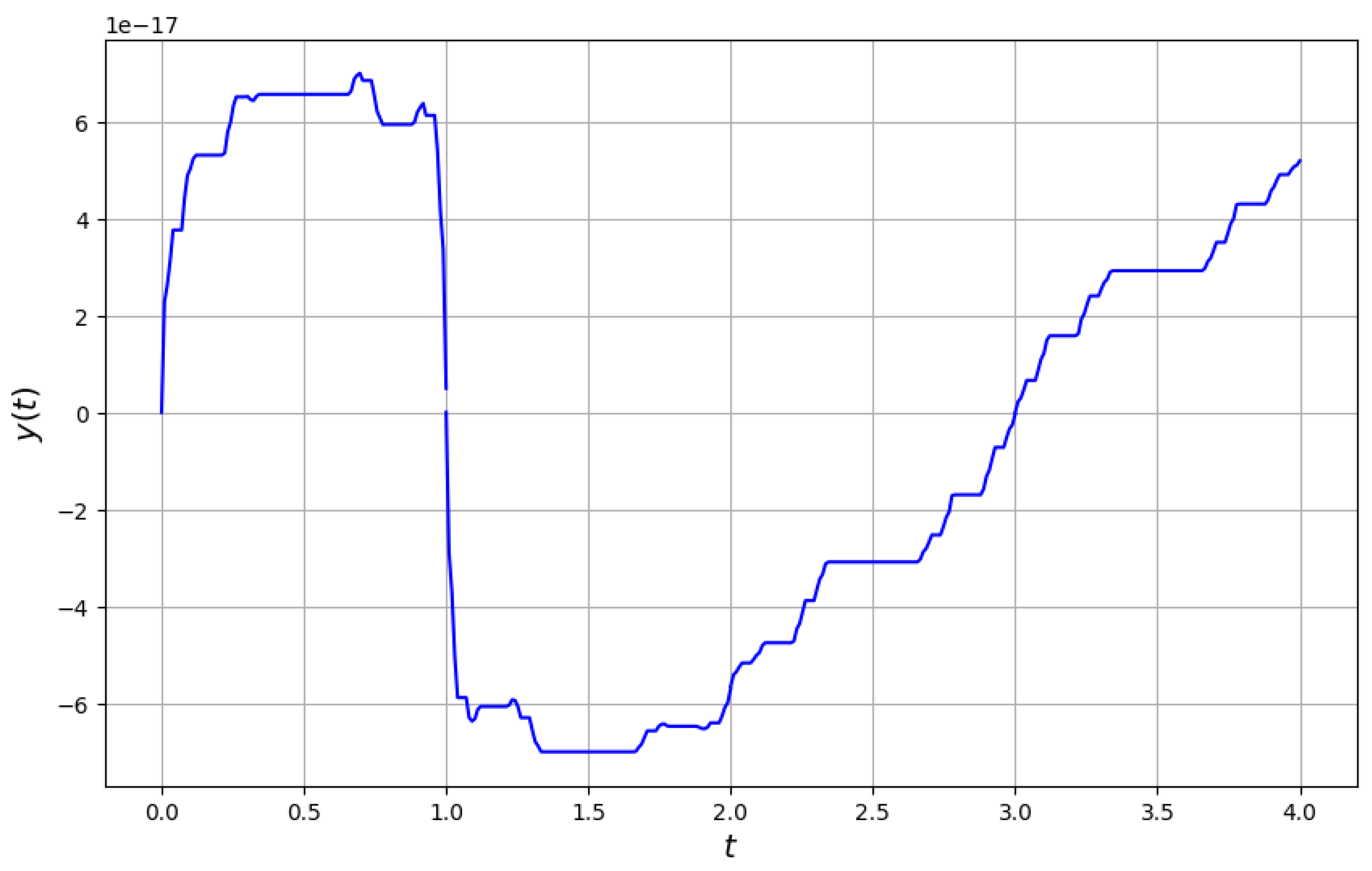
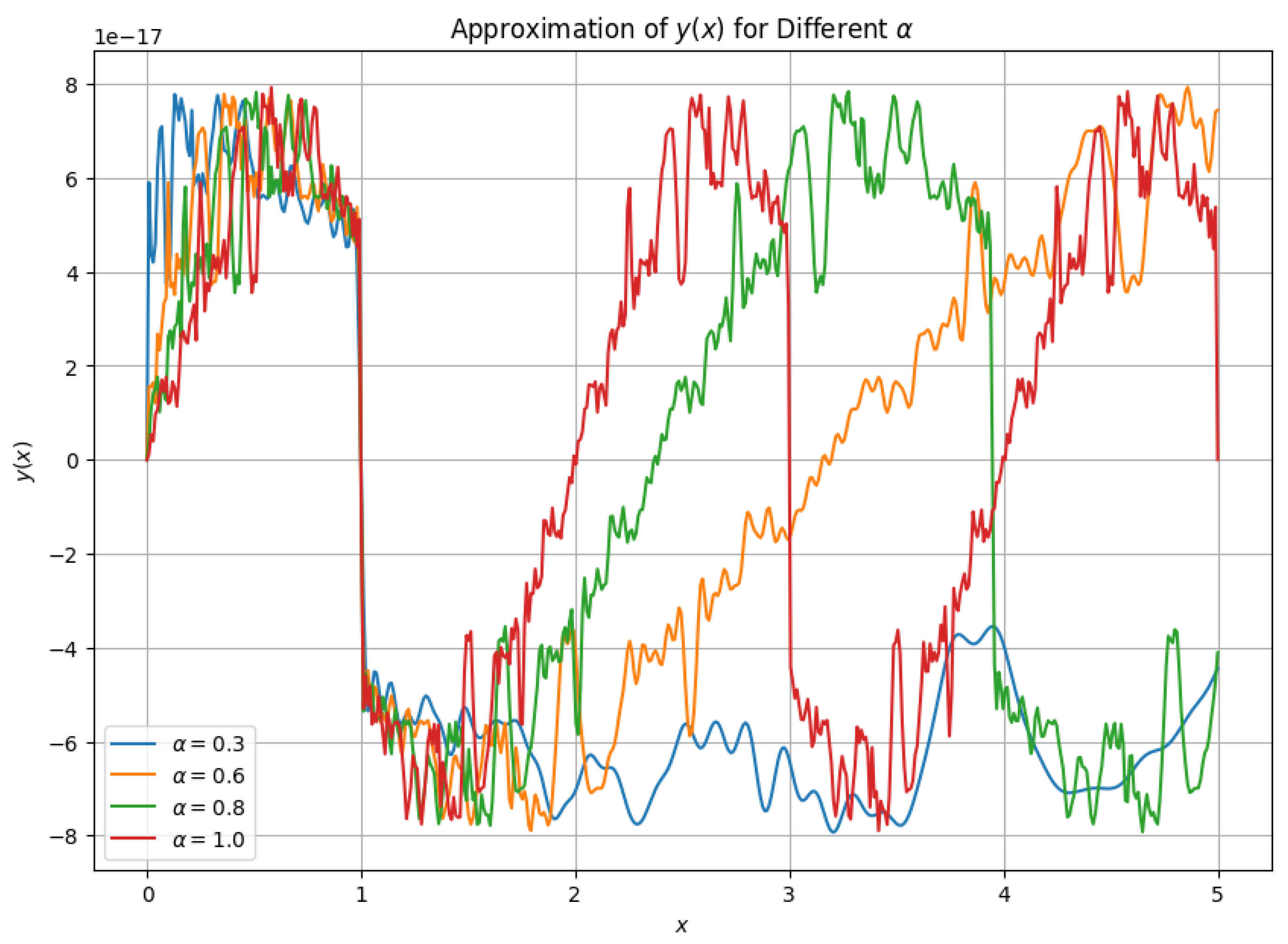
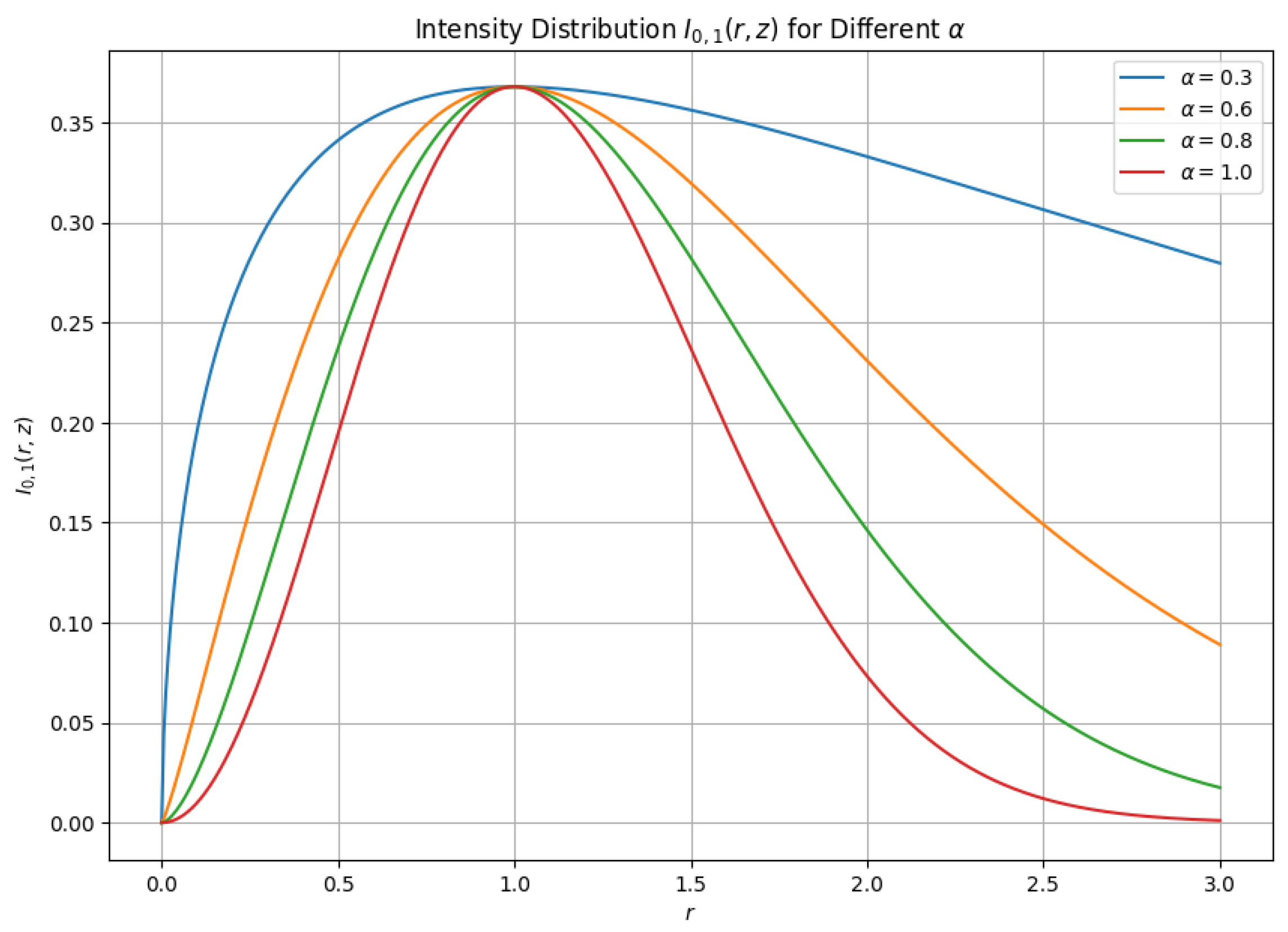
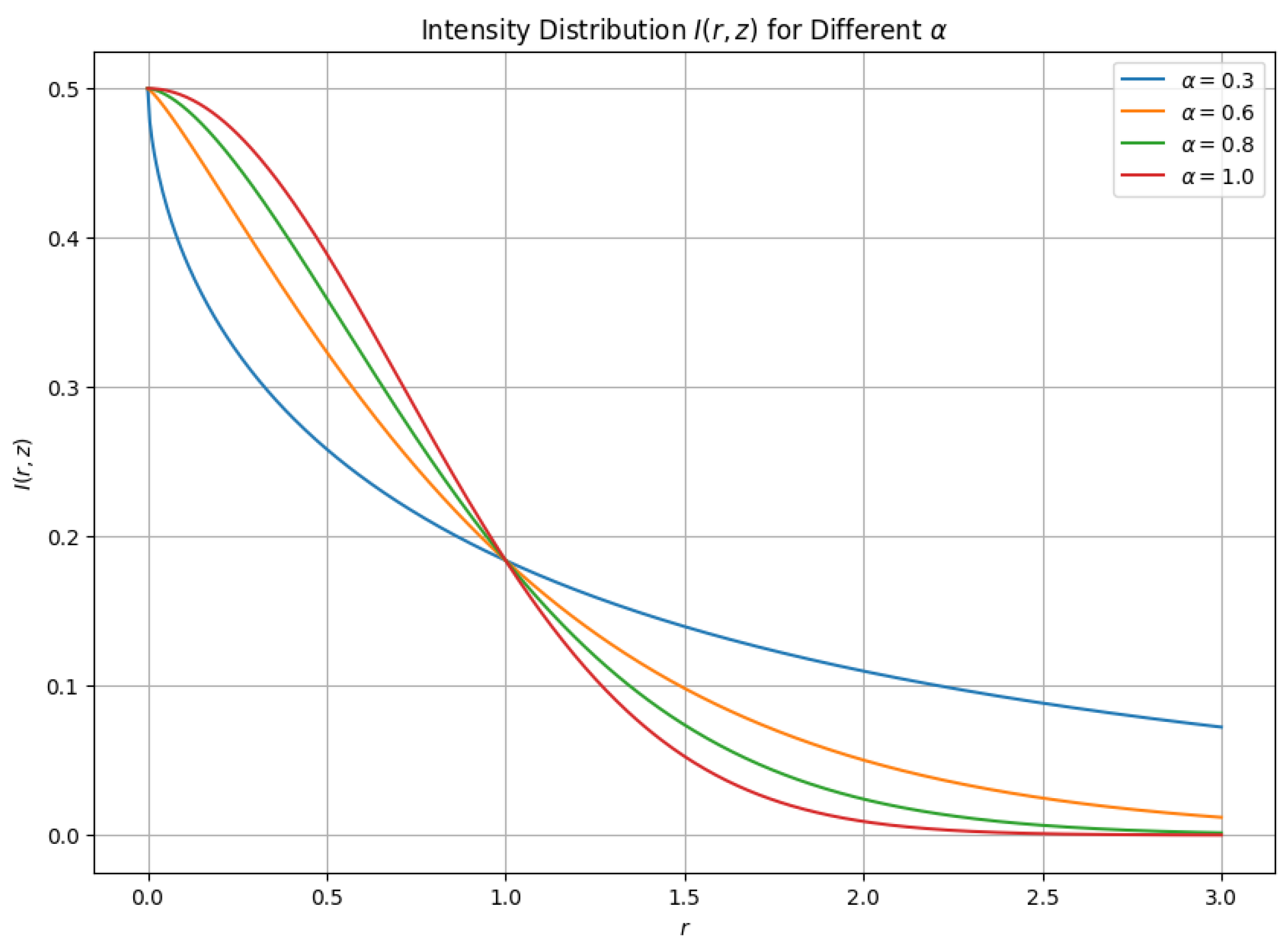
4. Applications

In this section, we explore the application of fractal Sturm–Liouville theory. The Laguerre–Gaussian (LG) modes, which are solutions to the paraxial wave equation in cylindrical coordinates [57,58,59,60], characterize the transverse intensity distributions of laser beams with circular symmetry. These modes play a fundamental role in optics [61,62,63], particularly in laser cavities and optical communication systems [64,65,66,67]. Here, we extend this framework to fractal Laguerre–Gaussian (FLG) modes, which are solutions to the fractal paraxial wave equation in cylindrical coordinates. Specifically, we consider the fractal paraxial Helmholtz equation [68] in cylindrical coordinates $(r,\theta ,z)$, where $r\in F$, given as follows:

$$D_{F,r}^{2\alpha }U+{\displaystyle \frac{1}{S_F^{\alpha }\left(r\right)}}{D}_{F,r}^{\alpha }U+{\displaystyle \frac{1}{S_F^{\alpha }{\left(r\right)}^2}}{\displaystyle \frac{{\partial }^{2}U}{\partial {\theta }^2}}+2ik{\displaystyle \frac{\partial U}{\partial z}}=0,$$

(47)

where $U(r,\theta ,z)$ is the complex amplitude of the optical field, and k is the wave number [61,69]. The solutions to Equation (47) are the fractal Laguerre–Gaussian modes [70], which are given as follows:

$$\begin{array}{cc}\hfill U_{p,l}(r,\theta ,z)& =C_{p,l}{\displaystyle \frac{w_0}{w\left(z\right)}}{\left({\displaystyle \frac{\sqrt{2}{S}_F^{\alpha }\left(r\right)}{w\left(z\right)}}\right)}^{|l|}\hfill \end{array}$$

$$\begin{array}{cc}\hfill & L_p^{(|l|)}\left({\displaystyle \frac{2S_F^{\alpha }{\left(r\right)}^2}{w^2\left(z\right)}}\right)\exp \left(-{\displaystyle \frac{S_F^{\alpha }{\left(r\right)}^2}{w^2\left(z\right)}}\right)\exp \left(il\theta \right)\exp \left(i{\psi }_{p,l}\left(z\right)\right)\hfill \\ & \approx C_{p,l}{\displaystyle \frac{w_0}{w\left(z\right)}}{\left({\displaystyle \frac{\sqrt{2}{r}^{\alpha }}{w\left(z\right)}}\right)}^{|l|}\hfill \end{array}$$

(48)

$$\begin{array}{cc}\hfill & L_p^{(|l|)}\left({\displaystyle \frac{2r^{2\alpha }}{w^2\left(z\right)}}\right)\exp \left(-{\displaystyle \frac{r^{2\alpha }}{w^2\left(z\right)}}\right)\exp \left(il\theta \right)\exp \left(i{\psi }_{p,l}\left(z\right)\right)\hfill \end{array}$$

(49)

where p is the radial index (non-negative integer), l is the azimuthal index (integer, representing orbital angular momentum), $L_p^{(|l|)}\left(x\right)$ are the associated Laguerre polynomials, $w\left(z\right)=w_0\sqrt{1+{\left({\displaystyle \frac{z}{z_R}}\right)}^2}$ is the beam radius, $z_R={\displaystyle \frac{\pi w_0^2}{\lambda }}$ is the Rayleigh range, ${\psi }_{p,l}\left(z\right)=(2p+|l|+1){\tan }^{-1}\left({\displaystyle \frac{z}{z_R}}\right)$ is the Gouy phase [71], and $C_{p,l}$ is a normalization constant. For the fractal fundamental mode, we have the following:

$$I_{0,0}(r,z)={\left|U_{0,0}(r,z)\right|}^2=I_0{\left({\displaystyle \frac{w_0}{w\left(z\right)}}\right)}^2\exp \left(-{\displaystyle \frac{2S_F^{\alpha }{\left(r\right)}^2}{w^2\left(z\right)}}\right),$$

where $I_0$ is the peak intensity. The beam exhibits a fractal Gaussian intensity profile. For the fractal vortex mode, we have the following:

$$\begin{array}{cc}\hfill I_{0,1}(r,z)& \propto S_F^{\alpha }{\left(r\right)}^2\exp \left(-{\displaystyle \frac{2S_F^{\alpha }{\left(r\right)}^2}{w^2\left(z\right)}}\right)\hfill \end{array}$$

(50)

$$\begin{array}{cc}& \approx r^{2\alpha }\exp \left(-{\displaystyle \frac{2r^{2\alpha }}{w^2\left(z\right)}}\right)\hfill \end{array}$$

(51)

which reveals a doughnut-shaped intensity pattern [72] due to the phase singularity at the center.

As shown in Figure 3, the intensity distribution $I_{0,1}(r,z)$ varies with the fractal dimension $\alpha$. The plot demonstrates that as $\alpha$ increases, the peak of the distribution becomes sharper and shifts closer to the center ($r=0$), indicating a more localized intensity profile. This behavior underscores the influence of the fractal parameter $\alpha$ on the spatial structure of the beam.

$$\begin{array}{cc}\hfill U_{0,0}(r,\theta ,z)& =C_{0,0}{\displaystyle \frac{w_0}{w\left(z\right)}}\exp \left(-{\displaystyle \frac{S_F^{\alpha }{\left(r\right)}^2}{w^2\left(z\right)}}\right)\exp \left(i{\psi }_{0,0}\left(z\right)\right),\hfill \end{array}$$

(52)

where r is the radial distance, $\theta$ is the azimuthal angle, z is the propagation distance along the beam axis, $w_0$ is the beam waist [73] at $z=0$, and $w\left(z\right)$ is the beam radius at a distance z from the waist, given as follows:

$$w\left(z\right)=w_0\sqrt{1+{\left({\displaystyle \frac{z}{z_R}}\right)}^2},$$

where $z_R={\displaystyle \frac{\pi w_0^2}{\lambda }}$ is the Rayleigh range, and ${\psi }_{0,0}\left(z\right)=(2p+|l|+1){\tan }^{-1}\left({\displaystyle \frac{z}{z_R}}\right)$ is the Gouy phase [74,75]. For the fundamental mode, the radial and azimuthal indices are both zero ($p=0$ and $l=0$), so the expression simplifies to the following:

$$\begin{array}{cc}\hfill U_{0,0}(r,z)& =C_{0,0}{\displaystyle \frac{w_0}{w\left(z\right)}}\exp \left(-{\displaystyle \frac{S_F^{\alpha }{\left(r\right)}^2}{w^2\left(z\right)}}\right)\hfill \end{array}$$

(53)

$$\begin{array}{cc}& \approx C_{0,0}{\displaystyle \frac{w_0}{w\left(z\right)}}\exp \left(-{\displaystyle \frac{r^{2\alpha }}{w^2\left(z\right)}}\right)\hfill \end{array}$$

(54)

The intensity distribution is the square of the absolute value of the complex field:

$$\begin{array}{cc}\hfill I(r,z)& =|U_{0,0}{(r,z)|}^2={\left|C_{0,0}{\displaystyle \frac{w_0}{w\left(z\right)}}\exp \left(-{\displaystyle \frac{S_F^{\alpha }{\left(r\right)}^2}{w^2\left(z\right)}}\right)\right|}^2\hfill \end{array}$$

(55)

The intensity distribution as a function of r and z is therefore given as follows:

$$\begin{array}{cc}\hfill I(r,z)& =|C_{0,0}{|}^2{\displaystyle \frac{w_0^2}{w^2\left(z\right)}}\exp \left(-{\displaystyle \frac{2S_F^{\alpha }{\left(r\right)}^2}{w^2\left(z\right)}}\right)\hfill \end{array}$$

(56)

$$\begin{array}{cc}& \approx |C_{0,0}{|}^2{\displaystyle \frac{w_0^2}{w^2\left(z\right)}}\exp \left(-{\displaystyle \frac{2r^{2\alpha }}{w^2\left(z\right)}}\right).\hfill \end{array}$$

(57)

As shown in Figure 4, the intensity distribution $I(r,z)$ varies with the fractal dimension $\alpha$. It is observed that as $\alpha$ increases, the intensity profile becomes more concentrated near $r=0$, indicating a sharper beam profile.

This distribution describes a Gaussian beam whose width increases with z, and the intensity decays exponentially with the square of the radial distance from the beam center. The beam waist $w_0$ corresponds to the point where the beam has its minimum radius, and the Rayleigh range [76] $z_R$ is the distance at which the beam radius has increased by a factor of $\sqrt{2}$.

Remark 4.

We note that throughout the paper, we find the solution to the fractal differential equation via conjugacy with ordinary calculus and fractal calculus [50].

Remark 5.

Fractal calculus provides a mathematical model for describing physical processes occurring in fractal media. Since fractal subsets of the real line represent the simplest types of fractal structures, the use of $F^{\alpha }$-calculus offers an algorithmic framework that can be generalized to more complex fractal geometries. The notion of the fractal dimension in this context, denoted by α, differs from classical dimensions such as the Hausdorff and box-counting dimensions. Specifically, the fractal dimension defined in $F^{\alpha }$-calculus typically satisfies the following inequality:

$${\dim }_H<\alpha <{\dim }_B,$$

where ${\dim }_H$ and ${\dim }_B$ denote the Hausdorff and box dimensions, respectively (see [23]).

5. Conclusions

In conclusion, this paper provides a comprehensive overview of fractal calculus and its application to generalized Sturm–Liouville theory. We introduced both the fractal homogeneous and non-homogeneous Sturm–Liouville problems, emphasizing their significance in the context of fractal spaces. This paper explored the theoretical framework and practical applications of these problems, particularly focusing on their relevance in optics. Through detailed examples and accompanying graphs, we demonstrated the impact of fractal support on the solutions, illustrating how fractal structures influence the behavior of differential equations. Furthermore, we proposed new models for fractal structures, expanding the understanding of their role in various physical and mathematical contexts. These findings offer valuable insights into the interaction between fractal geometry and differential equations, opening avenues for further research and applications in diverse fields.

References

- Falconer, K. Fractal Geometry: Mathematical Foundations and Applications; John Wiley & Sons: Hoboken, NJ, USA, 2004. [Google Scholar]
- Jorgensen, P.E. Analysis and Probability: Wavelets, Signals, Fractals; Springer Science & Business Media: Berlin/Heidelberg, Germany, 2006; Volume 234. [Google Scholar]
- Mandelbrot, B.B. The Fractal Geometry of Nature; WH Freeman New York: New York, NY, USA, 1982. [Google Scholar]
- Brown, C.; Liebovitch, L. Fractal Analysis; Sage: Newcastle upon Tyne, UK, 2010; Volume 165. [Google Scholar]
- Moreira, O. Fractal Analysis; Arcler Press: Burlington, ON, Canada, 2021. [Google Scholar]
- Kunze, H.; La Torre, D.; Mendivil, F.; Vrscay, E.R. Fractal-Based Methods in Analysis; Springer Science & Business Media: Berlin/Heidelberg, Germany, 2011. [Google Scholar]
- Lowen, S.B.; Teich, M.C. Fractal-Based Point Processes; John Wiley & Sons: Hoboken, NJ, USA, 2005. [Google Scholar]
- Kozlov, G.; Mikitaev, A.K.; Zaikov, G.E. The Fractal Physics of Polymer Synthesis; CRC Press: Boca Raton, FL, USA, 2013. [Google Scholar]
- Feder, J. Fractals; Springer Science & Business Media: Berlin/Heidelberg, Germany, 2013. [Google Scholar]
- West, B.J.; Grigolini, P.; Bologna, M. Fractal Calculus for CERTs. In Crucial Event Rehabilitation Therapy: Multifractal Medicine; Springer: Berlin/Heidelberg, Germany, 2023; pp. 69–83. [Google Scholar]
- Cross, S.S. Fractals in pathology. J. Pathol. 1997, 182, 1–8. [Google Scholar] [CrossRef]
- Sugihara, G.; May, R.M. Applications of fractals in ecology. Trends Ecol. Evol. 1990, 5, 79–86. [Google Scholar] [CrossRef]
- Bunde, A.; Havlin, S. Fractals in Science; Springer: Berlin/Heidelberg, Germany, 2013. [Google Scholar]
- Sandev, T.; Tomovski, Ž. Fractional Equations and Models; Springer International Publishing: Berlin/Heidelberg, Germany, 2019. [Google Scholar]
- Kigami, J. Analysis on Fractals; Number 143; Cambridge University Press: Cambridge, UK, 2001. [Google Scholar]
- Giona, M. Fractal calculus on [0, 1]. Chaos Solit. Fractals 1995, 5, 987–1000. [Google Scholar] [CrossRef]
- Freiberg, U.; Zähle, M. Harmonic calculus on fractals-a measure geometric approach I. Potential Anal. 2002, 16, 265–277. [Google Scholar] [CrossRef]
- Jiang, H.; Su, W. Some fundamental results of calculus on fractal sets. Commun. Nonlinear Sci. Numer. Simul. 1998, 3, 22–26. [Google Scholar] [CrossRef]
- Bongiorno, D.; Corrao, G. On the fundamental theorem of calculus for fractal sets. Fractals 2015, 23, 1550008. [Google Scholar] [CrossRef]
- Contreras, H.; Luis, F.; Galvis, J. Finite difference and finite element methods for partial differential equations on fractals. Rev. Integr. 2022, 40, 169–190. [Google Scholar] [CrossRef]
- Parvate, A.; Gangal, A.D. Calculus on fractal subsets of real line-I: Formulation. Fractals 2009, 17, 53–81. [Google Scholar] [CrossRef]
- Parvate, A.; Satin, S.; Gangal, A. Calculus on fractal curves in ℝn. Fractals 2011, 19, 15–27. [Google Scholar] [CrossRef]
- Golmankhaneh, A.K. Fractal Calculus and its Applications; World Scientific: Singapore, 2022. [Google Scholar]
- Golmankhaneh, A.K.; Cattani, C. Fractal logistic equation. Fractal Fract. 2019, 3, 41. [Google Scholar] [CrossRef]
- Banchuin, R. Noise analysis of electrical circuits on fractal set. COMPEL-Int. J. Comput. Math. Electr. Electron. Eng. 2022, 41, 1464–1490. [Google Scholar] [CrossRef]
- Banchuin, R. Nonlocal fractal calculus based analyses of electrical circuits on fractal set. COMPEL-Int. J. Comput. Math. Electr. Electron. Eng. 2022, 41, 528–549. [Google Scholar] [CrossRef]
- Banchuin, R. On the noise performances of fractal-fractional electrical circuits. Int. J. Circuit Theory Appl. 2023, 51, 80–96. [Google Scholar] [CrossRef]
- Balankin, A.S.; Mena, B. Vector differential operators in a fractional dimensional space, on fractals, and in fractal continua. Chaos Solit. Fractals 2023, 168, 113203. [Google Scholar] [CrossRef]
- Golmankhaneh, A.K.; Bongiorno, D. Exact solutions of some fractal differential equations. Appl. Math. Comput. 2024, 472, 128633. [Google Scholar] [CrossRef]
- Megías, E.; Golmankhaneh, A.K.; Deppman, A. Dynamics in fractal spaces. Phys. Lett. B 2024, 848, 138370. [Google Scholar] [CrossRef]
- Golmankhaneh, A.K.; Ontiveros, L.A.O. Fractal calculus approach to diffusion on fractal combs. Chaos Solit. Fractals 2023, 175, 114021. [Google Scholar] [CrossRef]
- Golmankhaneh, A.K.; Welch, K.; Serpa, C.; Jørgensen, P.E. Fuzzification of Fractal Calculus. arXiv 2023, arXiv:2302.07641. [Google Scholar]
- Golmankhaneh, A.K.; Jørgensen, P.E.; Schlichtinger, A.M. Einstein Field Equations Extended to Fractal Manifolds: A Fractal Perspective. J. Geom. Phys. 2023, 196, 105081. [Google Scholar] [CrossRef]
- Golmankhaneh, A.K.; Welch, K.; Serpa, C.; Rodríguez-López, R. Fractal Laplace transform: Analyzing fractal curves. Int. J. Anal. 2024, 32, 1111–1137. [Google Scholar] [CrossRef]
- Butcher, J.C. Numerical Methods for Ordinary Differential Equations; John Wiley & Sons: Hoboken, NJ, USA, 2016. [Google Scholar]
- Dormand, J.R. Numerical Methods for Differential Equations: A Computational Approach; CRC Press: Boca Raton, FL, USA, 2018. [Google Scholar]
- Cetinkaya, F.A.; Golmankhaneh, A.K. General characteristics of a fractal Sturm-Liouville problem. Turk. J. Math. 2021, 45, 1835–1846. [Google Scholar] [CrossRef]
- Allahverdiev, B.; Tuna, H. Existence theorem for a fractal Sturm–Liouville problem. Vladikavkaz Math. J. 2024, 26, 27–35. [Google Scholar]
- Nuckolls, K.P.; Scheer, M.G.; Wong, D.; Oh, M.; Lee, R.L.; Herzog-Arbeitman, J.; Watanabe, K.; Taniguchi, T.; Lian, B.; Yazdani, A. Spectroscopy of the fractal Hofstadter energy spectrum. Nature 2025, 639, 60–66. [Google Scholar] [CrossRef]
- Al-Gwaiz, M.A. Sturm-Liouville Theory and Its Applications; Springer: Berlin/Heidelberg, Germany, 2008; Volume 264. [Google Scholar]
- Zettl, A. Sturm-Liouville Theory; Number 121; American Mathematical Society: Providence, RI, USA, 2012. [Google Scholar]
- Lützen, J.; Lützen, J. Sturm-Liouville Theory. In Joseph Liouville 1809–1882: Master of Pure and Applied Mathematics; Springer Science & Business Media: Berlin/Heidelberg, Germany, 1990; pp. 423–475. [Google Scholar]
- Amrein, W.O.; Hinz, A.M.; Pearson, D.B. Sturm-Liouville Theory: Past and Present; Springer Science & Business Media: Berlin/Heidelberg, Germany, 2005. [Google Scholar]
- Fattorini, H.O. Second Order Linear Differential Equations in Banach Spaces; Elsevier: Amsterdam, The Netherlands, 2011; Volume 108. [Google Scholar]
- Levitan, B.M.; Sargsyan, I.S. Some problems in the theory of a Sturm-Liouville equation. Russ. Math. Surv. 1960, 15, 1. [Google Scholar] [CrossRef]
- Ames, W.F. Numerical Methods for Partial Differential Equations; Academic Press: Cambridge, MA, USA, 2014. [Google Scholar]
- Arfken, G.B.; Weber, H.J.; Harris, F.E. Mathematical Methods for Physicists: A Comprehensive Guide; Academic Press: Cambridge, MA, USA, 2011. [Google Scholar]
- Richtmyer, R.D.; Burdorf, C. Principles of Advanced Mathematical Physics; Springer: Berlin/Heidelberg, Germany, 1978; Volume 1. [Google Scholar]
- Naimark, M.A. Linear Differential Operators; Harrap: New York, NY, USA, 1968. [Google Scholar]
- Parvate, A.; Gangal, A. Calculus on fractal subsets of real line-II: Conjugacy with ordinary calculus. Fractals 2011, 19, 271–290. [Google Scholar] [CrossRef]
- Zizler, P.; Taylor, K.F.; Arimoto, S. The Courant-Fischer theorem and the spectrum of selfadjoint block band Toeplitz operators. Integral Eqs. Oper. Theory 1997, 28, 245–250. [Google Scholar] [CrossRef]
- Spielman, D. Spectral graph theory. In Combinatorial Scientific Computing; Chapman and Hall/CRC: Boca Raton, FL, USA, 2012; Volume 18. [Google Scholar]
- Golmankhaneh, A.K.; Depollier, C.; Pham, D. Higher order fractal differential equations. Mod. Phys. Lett. A 2024, 39, 2450127. [Google Scholar] [CrossRef]
- Boyce, W.E.; DiPrima, R.C.; Meade, D.B. Elementary Differential Equations and Boundary Value Problems; John Wiley & Sons: Hoboken, NJ, USA, 2021. [Google Scholar]
- Triebel, H. Analysis and Mathematical Physics; Springer Science & Business Media: Berlin/Heidelberg, Germany, 1987; Volume 24. [Google Scholar]
- Serov, V. Fourier Series, Fourier Transform and Their Applications to Mathematical Physics; Springer: Berlin/Heidelberg, Germany, 2017; Volume 197. [Google Scholar]
- Jordan, R.H.; Hall, D.G. Free-space azimuthal paraxial wave equation: The azimuthal Bessel–Gauss beam solution. Opt. Lett. 1994, 19, 427–429. [Google Scholar] [CrossRef]
- Kiselev, A. Localized light waves: Paraxial and exact solutions of the wave equation (a review). Opt. Spectrosc. 2007, 102, 603–622. [Google Scholar] [CrossRef]
- Kimel, I.; Elias, L.R. Relations between hermite and laguerre gaussian modes. IEEE J. Quantum Electron. 1993, 29, 2562–2567. [Google Scholar] [CrossRef]
- Kennedy, S.A.; Szabo, M.J.; Teslow, H.; Porterfield, J.Z.; Abraham, E. Creation of Laguerre-Gaussian laser modes using diffractive optics. Phys. Rev. A 2002, 66, 043801. [Google Scholar] [CrossRef]
- Bennett, C.A. Principles of Physical Optics; John Wiley & Sons: Hoboken, NJ, USA, 2022. [Google Scholar]
- Cocotos, V.; Mkhumbuza, L.; Forbes, K.A.; Koch, R.d.M.; Dudley, A.; Nape, I. Laguerre-Gaussian modes become elegant after an azimuthal phase modulation. arXiv 2024, arXiv:2411.07655. [Google Scholar] [CrossRef]
- Wei, D.; Cheng, Y.; Ni, R.; Zhang, Y.; Hu, X.; Zhu, S.; Xiao, M. Generating controllable Laguerre-Gaussian laser modes through intracavity spin-orbital angular momentum conversion of light. Phys. Rev. Appl. 2019, 11, 014038. [Google Scholar] [CrossRef]
- Plick, W.N.; Krenn, M. Physical meaning of the radial index of Laguerre-Gauss beams. Phys. Rev. A 2015, 92, 063841. [Google Scholar] [CrossRef]
- Valencia, N.H.; Srivastav, V.; Leedumrongwatthanakun, S.; McCutcheon, W.; Malik, M. Entangled ripples and twists of light: Radial and azimuthal Laguerre–Gaussian mode entanglement. J. Opt. 2021, 23, 104001. [Google Scholar] [CrossRef]
- Kovalev, A.; Kotlyar, V.; Porfirev, A. Asymmetric laguerre-gaussian beams. Phys. Rev. A 2016, 93, 063858. [Google Scholar] [CrossRef]
- Ghaderi Goran Abad, M.; Mahmoudi, M. Laguerre-Gaussian modes generated vector beam via nonlinear magneto-optical rotation. Sci. Rep. 2021, 11, 5972. [Google Scholar] [CrossRef]
- Shen, C. Riemann solutions and wave interactions for a hyperbolic system derived from the steady 2D Helmholtz equation under a paraxial assumption. Appl. Math. Lett. 2025, 160, 109320. [Google Scholar] [CrossRef]
- Verma, R.K. Wave Optics; Discovery Publishing House: Delhi, India, 2006. [Google Scholar]
- Fontaine, N.K.; Ryf, R.; Chen, H.; Neilson, D.T.; Kim, K.; Carpenter, J. Laguerre-Gaussian mode sorter. Nat. Commun. 2019, 10, 1865. [Google Scholar] [CrossRef]
- Feng, S.; Winful, H.G. Physical origin of the Gouy phase shift. Opt. Lett. 2001, 26, 485–487. [Google Scholar] [CrossRef]
- Züchner, T.; Failla, A.V.; Meixner, A.J. Light microscopy with doughnut modes: A concept to detect, characterize, and manipulate individual nanoobjects. Angew. Chem. Int. Ed. 2011, 50, 5274–5293. [Google Scholar] [CrossRef] [PubMed]
- Chapple, P.B. Beam waist and M2 measurement using a finite slit. Opt. Eng. 1994, 33, 2461–2466. [Google Scholar] [CrossRef]
- Hariharan, P.; Robinson, P. The Gouy phase shift as a geometrical quantum effect. J. Mod. Opt. 1996, 43, 219–221. [Google Scholar]
- Hiekkamäki, M.; Barros, R.F.; Ornigotti, M.; Fickler, R. Observation of the quantum Gouy phase. Nat. Photonics 2022, 16, 828–833. [Google Scholar] [CrossRef]
- Ji, X.; Dou, L. Two types of definitions for Rayleigh range. Opt. Laser Technol. 2012, 44, 21–25. [Google Scholar] [CrossRef]
Disclaimer/Publisher’s Note: The statements, opinions and data contained in all publications are solely those of the individual author(s) and contributor(s) and not of MDPI and/or the editor(s). MDPI and/or the editor(s) disclaim responsibility for any injury to people or property resulting from any ideas, methods, instructions or products referred to in the content. |
© 2025 by the authors. Licensee MDPI, Basel, Switzerland. This article is an open access article distributed under the terms and conditions of the Creative Commons Attribution (CC BY) license (https://creativecommons.org/licenses/by/4.0/).
Share and Cite
Golmankhaneh, A.K.; Vidović, Z.; Tuna, H.; Allahverdiev, B.P. Fractal Sturm–Liouville Theory. Fractal Fract. 2025, 9, 268. https://doi.org/10.3390/fractalfract9050268
Golmankhaneh AK, Vidović Z, Tuna H, Allahverdiev BP. Fractal Sturm–Liouville Theory. Fractal and Fractional. 2025; 9(5):268. https://doi.org/10.3390/fractalfract9050268
Chicago/Turabian StyleGolmankhaneh, Alireza Khalili, Zoran Vidović, Hüseyin Tuna, and Bilender P. Allahverdiev. 2025. "Fractal Sturm–Liouville Theory" Fractal and Fractional 9, no. 5: 268. https://doi.org/10.3390/fractalfract9050268
APA StyleGolmankhaneh, A. K., Vidović, Z., Tuna, H., & Allahverdiev, B. P. (2025). Fractal Sturm–Liouville Theory. Fractal and Fractional, 9(5), 268. https://doi.org/10.3390/fractalfract9050268