On the Laplace Residual Series Method and Its Application to Time-Fractional Fisher’s Equations

Abstract

In this paper, we develop an analytical approximate solution for the nonlinear time-fractional Fisher’s equation using a right starting space function and a unique analytic-numeric technique referred to as the Laplace residual power series approach. The generalized Taylor’s formula and the Laplace transform operator are coupled in the aforementioned method, where the coefficients, obtained through fractional expansion in the Laplace space, are determined by applying the limit concept. In order to validate and illustrate the theoretical methodology of the LRPS technique, as well as to show its effectiveness, adaptability, and superiority in solving various types of nonlinear time and space fractional differential equations, numerical experiments are generated. The obtained analytical solutions are compatible with the precise solutions and concur with those proposed by the other approaches. The outcomes show that the Laplace residual power series strategy is incredibly successful, straightforward to implement, and well suited for handling the complexity of nonlinear problems.

1. Introduction

The modeling of physical phenomena requires a comprehensive understanding of both current and past events. This has led to the widespread use of fractional calculus in various fields such as fluid mechanics, chemistry, biology, and psychology [1,2,3,4]. The concept of fractional calculus has been studied since 1695 and has gained significant interest from researchers and mathematicians in different scientific disciplines [5,6,7,8,9,10,11]. Several definitions of fractional derivatives and integrals have been developed over time, with Caputo’s formulation being widely adopted due to its practical applicability in real-world scenarios [12,13]. To accurately model a wide range of physical processes, there has been growing interest in solving fractional differential equations, particularly partial differential equations (PDEs) of the fractional order. This increasing attention stems from the ability of fractional calculus to better describe memory and hereditary properties in various scientific applications. As a result, numerous researchers have explored various methods, both analytical and numerical, to obtain approximate or close solutions for these equations. Several well-established techniques have been widely used, including the Laplace transform method [14], the Adomian decomposition method [15], the multi-step fractional differential transform method [16], the variational iteration method [17], the homotopy perturbation method [18], the reproducing kernel method [19], and the residual power series (RPS) method [20]. These techniques have shown significant effectiveness in the treatment of complex fractional differential equations in various domains [21,22,23].

The development and utilization of these methods highlight the ongoing research efforts aimed at effectively solving complex problems arising from the PDEs of fractional order. The RPS method is a highly effective technique for finding approximate series solutions to both fractional and non-fractional differential equations. It has been extensively tested and proven successful in solving various differential equations, including the nonlinear Kuramoto–Sivashinsky equation [20], neutron diffusion equations [24], fractional Newell–Whitehead–Segel equation [25], fractional-order coupled system of PEDs [26], and fractional logistic equation [27].

The simplicity and effectiveness of the RPS approach in determining the coefficients of the power series solution make it unique. This is especially crucial when working with nonlinear equations. The Laplace residual power series (LRPS) approach is a novel RPS method introduced by the authors in [28] in a recent paper. In this innovative technique, instead of relying on derivatives to determine coefficients, the authors utilized the concept of limits. This modification significantly enhanced both the speed and ease of determining coefficients while providing solutions in the form of converging series without resorting to linearization, perturbation, or discretization techniques. The introduction of the LRPS method opens up new possibilities for the exact and approximate series solutions to linear and nonlinear neutral fractional differential equations.

It is worth emphasizing that the LRPS expansion technique derives a solution by converting the differential equation into the Laplace domain. To obtain the solution for the original problem, the inverse Laplace transform is applied, restoring it to its original space. In this work, the nonlinear time-fractional Fisher’s equation is approximated using the LRPS technique. Consider the time-fractional Fisher’s equation given below:

$${Ð}_t^{\gamma }\phi =D_x^2\phi +\lambda \phi (1-\phi ),x\in R,t\ge 0,$$

(1)

equipped with the initial data

$$\phi (x,0)={\theta }_0\left(x\right),$$

(2)

in which $\lambda$ is a constant, $\phi$ is an unknown function to be determined and ${Ð}_t^{\gamma }\phi$ is a $\gamma$-th time-Caputo fractional derivative.

The organization of this document is as follows: Section 2 provides an overview of the theory of fractional calculus. Section 3 introduces the FRPS method applied to solve the nonlinear time-fractional Fisher’s equation. Section 4 demonstrates the effectiveness of the LRPS technique through two illustrative examples. Finally, the conclusion is presented in the Section 5.

2. Fundamental Concepts

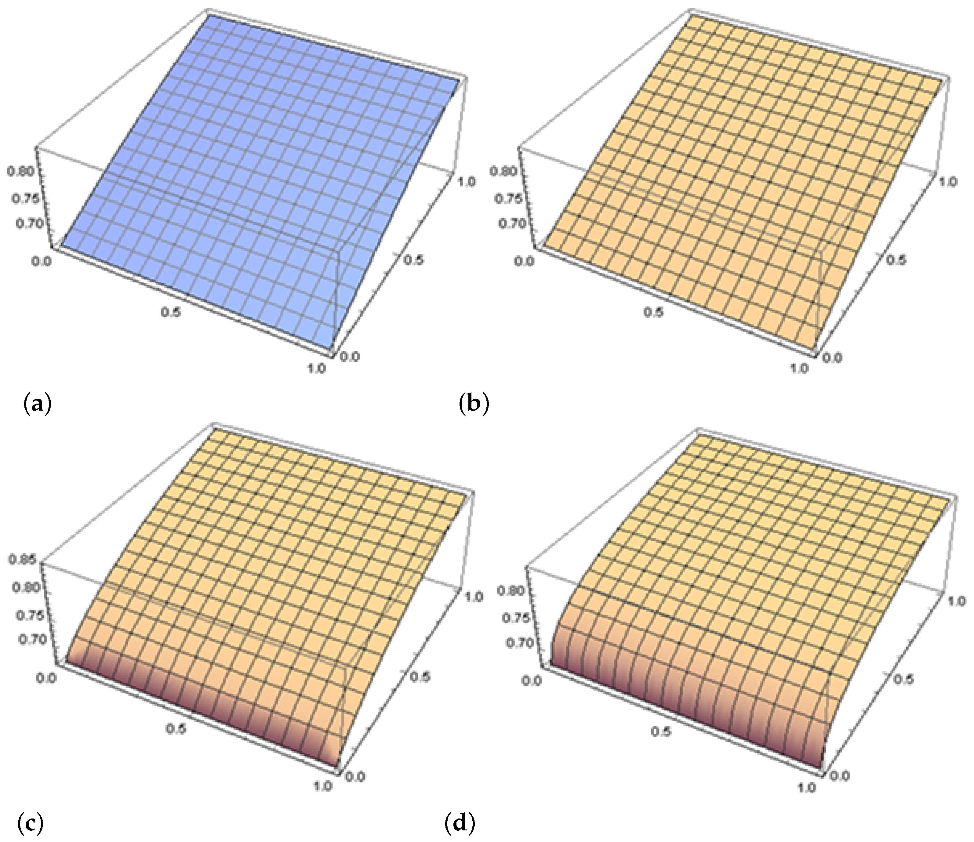
In this section, we provide an overview of the fundamental definitions of Laplace transform operators and fractional calculus. Additionally, we discuss the most essential characteristics of the fractional series expansion in the Laplace domain, along with Caputo operators and the Laplace transform [29,30,31,32,33,34].

Definition 1.

The Riemann–Liouville time-fractional integral operator of order $\gamma \ge 0$, denoted by $J_{\xi }^{\gamma }$, is given as

$$J_{\xi }^{\gamma }\phi (x,\xi )=\left\{\begin{array}{cc}{\displaystyle \frac{1}{\mathrm{\Gamma }\left(\gamma \right)}}{\displaystyle \underset{0}{\overset{\xi }{\int }}}{(\xi -\tau )}^{\gamma -1}\phi (x,\tau )d\tau ,\hfill & \gamma >0,\xi >\tau \ge 0\\ \phi (x,\xi ),\hfill & \gamma =0.\end{array}\right.$$

(3)

Definition 2.

For $m\in \mathbb{N}$, the time-fractional derivative ${Ð}_{\xi }^{\gamma }$ of $\phi (x,\xi )$ of order $\gamma >0$, in the meaning of Caputo is given by

$${Ð}_{\xi }^{\gamma }\phi (x,\xi )=J_t^{m-\gamma }{\partial }_{\xi }^m\phi (x,\xi ),m-1<\gamma \le m,x\in I,\xi \ge 0.$$

(4)

Definition 3.

Let $\phi (x,\xi )$ be a continuous piecewise function on $I\times [0,\infty )$, $\phi (x,\xi )$ is of exponential order δ, then the Laplace transform $\varphi (x,s)$ is given for $\phi (x,\xi )$ as

$$\varphi (x,s)=\mathcal{L}\left[\phi (x,\xi )\right]:={\displaystyle \underset{0}{\overset{\infty }{\int }}}{e}^{-s\xi }\phi (x,\xi )d\xi (s>\delta ),$$

(5)

while the inversion formula of the Laplace transform of ϕ is derived as

$$\varphi (x,\xi )={\mathcal{L}}^{-1}\left[\phi (x,s)\right]:={\displaystyle \underset{z-i\infty }{\overset{z+i\infty }{\int }}}{e}^{s\xi }\phi (x,s)ds,Re\left(s\right)>z_0.$$

(6)

The following lemma discusses some useful properties of the Laplace pair of transforms.

Lemma 1.

Let $\phi$ and ω be two functions which are piecewise continuous on $I\times [0,\infty )$. Let $\phi$ and ω be of the exponential orders ${\delta }_1$ and ${\delta }_2$, ${\delta }_1<{\delta }_2$, respectively, and $\mathcal{L}\left[\phi (x,\xi )\right]=\varphi (x,s),$$\mathcal{L}\left[\omega (x,\xi )\right]=W(x,s),$ and $a,b$ are constants. Then, for $x\in I,s>{\delta }_1,\xi \ge 0$, we have

(a) 

$\mathcal{L}\left[a\phi +b\omega \right]=a\varphi +bW.$

(b) 

${\mathcal{L}}^{-1}\left[a\varphi +bW\right]=a\phi +b\omega .$

(c) 

$\underset{s\to \infty }{lim}s\varphi (x,s)=\phi (x,0),x\in I.$

(d) 

$\mathcal{L}\left[{Ð}_{\xi }^{\gamma }\phi (x,\xi )\right]=s^{\gamma }\varphi (x,s)-{\displaystyle \sum _{k=0}^{m-1}}{s}^{\gamma -k-1}{\partial }_{\xi }^k\phi (x,0),m-1<\gamma <m.$

(e) 

$\mathcal{L}\left[{Ð}_{\xi }^{n\gamma }\phi (x,\xi )\right]=s^{n\gamma }\varphi (x,s)-{\displaystyle \sum _{k=0}^{n-1}}{s}^{(n-k)\gamma -1}{D}_{\xi }^{k\gamma }\phi (x,0),0<\gamma <1.$

Theorem 1.

Let $\phi (x,\xi )$ have a power series expansion of fractional order around $\xi =0$ such that

$$\phi (x,\xi )={\displaystyle \sum _{n=0}^{\infty }}{\theta }_n\left(x\right){\xi }^{n\gamma },0\le m-1<\gamma \le m,x\in I,0\le \xi <R.$$

(7)

Let ${Ð}_{\xi }^{n\gamma }\phi (x,\xi )$ be continuous on $I\times (0,\mathbb{R})$, $m=0,1,2,\dots$, then the coefficients ${\theta }_n\left(x\right)$ of the expansion $\left(7\right)$ are given as ${\theta }_n\left(x\right)$ = ${\displaystyle \frac{{Ð}_{\xi }^{n\gamma }\phi (x,0)}{\mathrm{\Gamma }(n\gamma +1)}}$, $n=0,1,2,\dots$, where ${Ð}_{\xi }^{n\gamma }$ = ${Ð}_{\xi }^{\gamma }$ ${Ð}_{\xi }^{\gamma }$ … ${Ð}_{\xi }^{\gamma }$($n-times$), and R is the radius of convergence of the given series.

Theorem 2.

Let the Laplace transform of the continuous function $\phi (x,\xi )$ be given by $\varphi (x,s)$. Then, $\varphi (x,s)$ has the fractional series expansion

$$\varphi (x,s)={\displaystyle \sum _{n=0}^{\infty }}{\displaystyle \frac{{\theta }_n\left(x\right)}{s^{1+n\alpha }}},0<\alpha \le 1,x\in I,s>\delta .$$

(8)

Theorem 3.

Let $\mathcal{L}\left[\phi (x,\xi )\right]=\varphi (x,s)$ be given by $\left(8\right)$. If $\left|s\mathcal{L}\left[{Ð}_{\xi }^{(n+1)\gamma }\gamma (x,\xi )\right]\right|\le M\left(x\right),$ defined on $I\times (\delta ,d]$, $0<\gamma \le 1$, then the reminder ${\Re }_n(x,s)$ satisfies the following inequality:

$$\left|{\Re }_n(x,s)\right|\le {\displaystyle \frac{M\left(x\right)}{s^{1+(n+1)\gamma }}},x\in I,\delta <s\le d.$$

(9)

3. The LRPS Method

This section describes the techniques employed in the proposed algorithm for resolving the fractional initial value problems (IVPs) (1) and (2) in series form. The method combines the Laplace transform operator with the fractional RPS approach. By employing these techniques, we aim to solve these IVPs systematically and efficiently. The proposed method follows the procedure outlined below:

First:

Let $\mathcal{L}\left[\phi (x,t)\right]=\varphi (x,s)$, and using property $\left(e\right)$ from Lemma 1, the Laplace transform can be applied to both sides of Fisher’s problem (1) to obtain

$$\varphi (x,s)={\displaystyle \frac{\phi (x,0)}{s}}+{\displaystyle \frac{1}{s^{\gamma }}}{D}_x^2\varphi (x,s)+{\displaystyle \frac{\lambda }{s^{\gamma }}}\varphi (x,s)-{\displaystyle \frac{\lambda }{s^{\gamma }}}\mathcal{L}\left\{{\mathcal{L}}^{-1}{\left[\varphi (x,s)\right]}^2\right\}.$$

(10)

Since $\phi (x,0)={\theta }_0\left(x\right)$. Thus, (10) can be reformulated as:

$$\varphi (x,s)={\displaystyle \frac{{\theta }_0\left(x\right)}{s}}+{\displaystyle \frac{1}{s^{\gamma }}}{D}_x^2\varphi (x,s)+{\displaystyle \frac{\lambda }{s^{\gamma }}}\varphi (x,s)-{\displaystyle \frac{\lambda }{s^{\gamma }}}\mathcal{L}\left\{{\mathcal{L}}^{-1}{\left[\varphi (x,s)\right]}^2\right\}.$$

(11)

Second:

According to Theorem 2, let the approximate solution of (11) have the expansion series form

$$\varphi (x,s)={\displaystyle \sum _{m=0}^{\infty }}{\displaystyle \frac{{\theta }_m\left(x\right)}{s^{m\gamma +1}}},s>0.$$

(12)

Subsequently, to determine the coefficients ${\theta }_m$, of (12), let ${\varphi }_i(x,s)$ be the i-th term of the series solution of (12). That is,

$${\varphi }_i(x,s)={\displaystyle \sum _{m=0}^i}{\displaystyle \frac{{\theta }_m\left(x\right)}{s^{m\gamma +1}}},s>0.$$

(13)

For $i=0$, we have $\underset{s\to \infty }{lim}$$s{\varphi }_0(x,s)={\theta }_0\left(x\right)$, which yields

$${\varphi }_i(x,s)={\displaystyle \frac{{\theta }_0\left(x\right)}{s}}+{\displaystyle \sum _{m=0}^i}{\displaystyle \frac{{\theta }_m\left(x\right)}{s^{m\gamma +1}}},s>0.$$

(14)

Third:

The i-th term of the series solution (14) can be obtained after evaluating the coefficients ${\theta }_m$, $m=1,2,3,\dots ,i,$ by identifying the i-th-Laplace residual function of (10) as

$$\begin{array}{cc}\mathcal{L}\left[Res{\varphi }_i(x,s)\right]\hfill & ={\varphi }_i(x,s)-{\displaystyle \frac{{\theta }_0\left(x\right)}{s}}-{\displaystyle \frac{1}{s^{\gamma }}}{D}_x^2{\varphi }_i(x,s)\hfill \\ \hfill & -{\displaystyle \frac{\lambda }{s^{\gamma }}}{\varphi }_i(x,s)+{\displaystyle \frac{\lambda }{s^{\gamma }}}\mathcal{L}\left\{{\mathcal{L}}^{-1}{\left[{\varphi }_i(x,s)\right]}^2\right\}.\hfill \end{array}$$

(15)

Here, the ∞-th Laplace residual function of (10) can be given by

$$\begin{array}{cc}\underset{i\to \infty }{lim}\mathcal{L}\left[Res{\varphi }_i(x,s)\right]\hfill & =\mathcal{L}\left[Res\varphi (x,s)\right]\hfill \\ \hfill & =\varphi (x,s)-{\displaystyle \frac{{\theta }_0\left(x\right)}{s}}-{\displaystyle \frac{1}{s^{\gamma }}}{D}_x^2\varphi (x,s)\hfill \\ \hfill & -{\displaystyle \frac{\lambda }{s^{\gamma }}}\varphi (x,s)+{\displaystyle \frac{\lambda }{s^{\gamma }}}\mathcal{L}\left\{{\mathcal{L}}^{-1}{\left[\varphi (x,s)\right]}^2\right\}.\hfill \end{array}$$

(16)

Evidently, $\mathcal{L}\left[Res\varphi (x,s)\right]=0$ and $\underset{i\to \infty }{lim}\mathcal{L}\left[Res{\varphi }_i(x,s)\right]=\mathcal{L}\left[Res\varphi (x,s)\right]$ for each $s>0$ and $x\in \mathbb{R}$. Furthermore, $\underset{s\to \infty }{lim}s\mathcal{L}\left[Res\varphi (x,s)\right]=0$, which implies that $\underset{s\to \infty }{lim}s\mathcal{L}\left[Res{\varphi }_i(x,s)\right]=0$.

Fourth:

After substituting the i-th term of the series solution (14) into the i-th Laplace residual function, both sides of the resulting equation are multiplied by the factor $s^{i\gamma +1}$.

Fifth:

To determine the coefficients ${\theta }_m\left(x\right)$, $m=1,2,3,\dots ,i,$ we solve $\underset{s\to \infty }{lim}{s}^{i\gamma +1}\mathcal{L}\left[Res{\varphi }_i(x,s)\right]=0$. Subsequently, by collecting the obtained coefficients into the expansion series (14), the i-th Laplace series solution ${\varphi }_i(x,s)$ of (11) is derived.

Sixth:

The approximate solution ${\phi }_i(x,t)$ of the IVPs (1) and (2) can be obtained by applying the Laplace transform inversion formula to both sides of the i-th Laplace solution ${\varphi }_i(x,s)$.

In view of the above, to determine the first coefficient ${\theta }_1\left(x\right)$ in the expansion (14), we have to substitute ${\varphi }_1(x,s)={\displaystyle \frac{{\theta }_0\left(x\right)}{s}}+{\displaystyle \frac{{\theta }_1\left(x\right)}{s^{\gamma +1}}}$ into the first Laplace residual function as follows

$$\begin{array}{cc}\mathcal{L}\left[Res{\varphi }_1(x,s)\right]\hfill & ={\varphi }_1(x,s)-{\displaystyle \frac{{\theta }_0\left(x\right)}{s}}-{\displaystyle \frac{1}{s^{\gamma }}}{D}_x^2{\varphi }_1(x,s)\hfill \\ \hfill & -{\displaystyle \frac{\lambda }{s^{\gamma }}}{\varphi }_1(x,s)+{\displaystyle \frac{\lambda }{s^{\gamma }}}\mathcal{L}\left\{{\mathcal{L}}^{-1}{\left[{\varphi }_1(x,s)\right]}^2\right\}\hfill \\ \hfill & ={\displaystyle \frac{{\theta }_1\left(x\right)}{s^{1+\gamma }}}-\lambda \left({\displaystyle \frac{{\theta }_0\left(x\right)}{s^{1+\gamma }}}+{\displaystyle \frac{{\theta }_1\left(x\right)}{s^{1+2\gamma }}}\right)\hfill \\ \hfill & +\lambda \left({\displaystyle \frac{{\theta }_0^2\left(x\right)}{s^{1+\gamma }}}+{\displaystyle \frac{2{\theta }_0\left(x\right){\theta }_1\left(x\right)}{s^{1+2\gamma }}}+{\displaystyle \frac{\mathrm{\Gamma }(1+2\gamma ){\theta }_1^2\left(x\right)}{{\mathrm{\Gamma }}^2(\gamma +1)s^{1+3\gamma }}}\right)\hfill \\ \hfill & -\left({\displaystyle \frac{{\theta }_0^{″}\left(x\right)}{s^{1+\gamma }}}+{\displaystyle \frac{{\theta }_1^{″}\left(x\right)}{s^{1+2\gamma }}}\right).\hfill \end{array}$$

(17)

Now, multiplying both sides of (17) by $s^{\gamma +1}$ gives

$$\begin{array}{cc}{s}^{\gamma +1}\mathcal{L}\left[Res{\varphi }_1(x,s)\right]\hfill & =-\lambda {\theta }_0\left(x\right)+\lambda {\theta }_0^2\left(x\right)+{\theta }_1\left(x\right)-{\displaystyle \frac{\lambda {\theta }_1\left(x\right)}{s^{\gamma }}}+{\displaystyle \frac{2\lambda {\theta }_0\left(x\right){\theta }_1\left(x\right)}{s^{\gamma }}}\hfill \\ \hfill & +{\displaystyle \frac{\mathrm{\Gamma }(1+2\gamma ){\theta }_1^2\left(x\right)}{{\mathrm{\Gamma }}^2(\gamma +1)s^{3\gamma }}}-{\theta }_0^{″}\left(x\right)-{\displaystyle \frac{{\theta }_1^{″}\left(x\right)}{s^{\gamma }}}.\hfill \end{array}$$

(18)

In light of the fact that $\underset{s\to \infty }{lim}{s}^{\gamma +1}\mathcal{L}\left[Res{\varphi }_1(x,s)\right]=0$, we obtain ${\theta }_1\left(x\right)=\lambda ({\theta }_0\left(x\right)-{\theta }_0^2\left(x\right))+{\theta }_0^{″}\left(x\right)$. To date, the first Laplace series solution ${\varphi }_1(x,s)$ of (11) has the form

$${\varphi }_1(x,s)={\displaystyle \frac{{\theta }_0\left(x\right)}{s}}+{\displaystyle \frac{\lambda ({\theta }_0\left(x\right)-{\theta }_0^2\left(x\right))+{\theta }_0^{″}\left(x\right)}{s^{\gamma +1}}}.$$

For $i=2$, the 2-nd Laplace series solution of (11) can be written as

$${\varphi }_2(x,s)={\displaystyle \frac{{\theta }_0\left(x\right)}{s}}+{\displaystyle \frac{{\theta }_1\left(x\right)}{s^{\gamma +1}}}+{\displaystyle \frac{{\theta }_2\left(x\right)}{s^{2\gamma +1}}}.$$

(19)

Thus, by substituting the series expansion from (19) into (15), we obtain

$$\begin{array}{cc}\mathcal{L}\left\{Res{\varphi }_2(x,s)\right\}\hfill & =-\lambda \left({\displaystyle \frac{{\theta }_0\left(x\right)}{s}}+{\displaystyle \frac{{\theta }_1\left(x\right)}{s^{\gamma +1}}}+{\displaystyle \frac{{\theta }_2\left(x\right)}{s^{2\gamma +1}}}\right)\hfill \\ \hfill & +\lambda ({\displaystyle \frac{2{\theta }_0\left(x\right){\theta }_1\left(x\right)}{s^{1+2\gamma }}}+{\displaystyle \frac{2{\theta }_0\left(x\right){\theta }_2\left(x\right)}{s^{1+3\gamma }}}+{\displaystyle \frac{\mathrm{\Gamma }(2\gamma +1){\theta }_1^2\left(x\right)}{{\mathrm{\Gamma }}^2(\gamma +1)s^{1+3\gamma }}}\hfill \\ \hfill & +{\displaystyle \frac{2\mathrm{\Gamma }(3\gamma +1){\theta }_1\left(x\right){\theta }_2\left(x\right)}{\mathrm{\Gamma }(\gamma +1)\mathrm{\Gamma }(2\gamma +1)s^{1+4\gamma }}}+{\displaystyle \frac{\mathrm{\Gamma }(4\gamma +1){\theta }_0^2\left(x\right)}{{\mathrm{\Gamma }}^2(2\gamma +1)s^{1+5\gamma }}}+{\displaystyle \frac{{\theta }_0^2\left(x\right)}{s^{1+\gamma }}})\hfill \\ \hfill & -\left({\displaystyle \frac{{\theta }_1^{″}\left(x\right)}{s^{1+2\gamma }}}+{\displaystyle \frac{{\theta }_2^{″}\left(x\right)}{s^{1+3\gamma }}}+{\displaystyle \frac{{\theta }_0^{″}\left(x\right)}{s^{1+\gamma }}}\right)+{\displaystyle \frac{{\theta }_1\left(x\right)}{s^{1+\gamma }}}+{\displaystyle \frac{{\theta }_2\left(x\right)}{s^{1+2\gamma }}}.\hfill \end{array}$$

(20)

Now, multiplying both sides of (20) by the factor $s^{1+2\gamma }$ reveals

$$\begin{array}{cc}{s}^{1+2\gamma }\mathcal{L}\left\{Res{\varphi }_2(x,s)\right\}\hfill & =-\lambda {\displaystyle \frac{{\theta }_2\left(x\right)}{s^{\gamma }}}+{\displaystyle \frac{2\lambda {\theta }_0\left(x\right){\theta }_2\left(x\right)}{s^{\gamma }}}+{\displaystyle \frac{\mathrm{\Gamma }(4\gamma +1){\theta }_2^2\left(x\right)}{{\mathrm{\Gamma }}^2(2\gamma +1)s^{3\gamma }}}\hfill \\ \hfill & +{\displaystyle \frac{2\lambda \mathrm{\Gamma }(3\gamma +1){\theta }_1\left(x\right){\theta }_2\left(x\right)}{\mathrm{\Gamma }(\gamma +1)\mathrm{\Gamma }(2\gamma +1)s^{2\gamma }}}+{\displaystyle \frac{\lambda \mathrm{\Gamma }(2\gamma +1){\theta }_1^2\left(x\right)}{{\mathrm{\Gamma }}^2(\gamma +1)s^{\gamma }}}-{\displaystyle \frac{{\theta }_2^{″}\left(x\right)}{s^{\gamma }}}+\lambda s^{\gamma }{\theta }_0^2\left(x\right)\hfill \\ \hfill & -\lambda s^{\gamma }{\theta }_0\left(x\right)-s^{\gamma }{\theta }_0^{″}\left(x\right)+s^{\gamma }{\theta }_1\left(x\right)-\lambda {\theta }_1\left(x\right)+2\lambda {\theta }_0\left(x\right){\theta }_1\left(x\right)-{\theta }_1^{″}\left(x\right)+{\theta }_2\left(x\right).\hfill \end{array}$$

(21)

By solving $\underset{s\to \infty }{lim}{s}^{1+2\gamma }\mathcal{L}\left[Res{\varphi }_2(x,s)\right]=0$, we obtain ${\theta }_2\left(x\right)=\lambda {\theta }_1\left(x\right)\left(1-2{\theta }_0\left(x\right)\right)+{\theta }_1^{″}\left(x\right)$. Hence, the second Laplace series solution can be given by ${\varphi }_2(x,s)=$${\displaystyle \frac{{\theta }_0\left(x\right)}{s}}+{\displaystyle \frac{\lambda {\theta }_0\left(x\right)(1-{\theta }_0\left(x\right))+{\theta }_0^{″}\left(x\right)}{s^{\gamma +1}}}+{\displaystyle \frac{\lambda {\theta }_1\left(x\right)\left(1-2{\theta }_0\left(x\right)\right)+{\theta }_1^{″}\left(x\right)}{s^{2\gamma +1}}}$.

Once again, for $i=3$, the 3-rd residual function of (11), $\mathcal{L}\left\{Res{\varphi }_3(x,s)\right\}$, can be written as

$$\begin{array}{cc}\mathcal{L}\left\{Res{\varphi }_3(x,s)\right\}\hfill & ={\varphi }_3(x,s)-{\displaystyle \frac{{\theta }_0\left(x\right)}{s}}-{\displaystyle \frac{1}{s^{\gamma }}}{D}_x^2{\varphi }_3(x,s)\hfill \\ \hfill & -{\displaystyle \frac{\lambda }{s^{\gamma }}}{\varphi }_3(x,s)+{\displaystyle \frac{\lambda }{s^{\gamma }}}\mathcal{L}\left\{{\mathcal{L}}^{-1}{\left[{\varphi }_3(x,s)\right]}^2\right\}.\hfill \end{array}$$

(22)

After substituting ${\varphi }_3(x,s)={\displaystyle \frac{{\theta }_0\left(x\right)}{s}}+{\displaystyle \frac{{\theta }_1\left(x\right)}{s^{\gamma +1}}}+{\displaystyle \frac{{\theta }_2\left(x\right)}{s^{2\gamma +1}}}+{\displaystyle \frac{{\theta }_3\left(x\right)}{s^{3\gamma +1}}}$ into (21), the resulting fractional equation is multiplied by $s^{3\gamma +1}$ to yield

$$\begin{array}{cc}{s}^{1+3\gamma }\mathcal{L}\left\{Res{\varphi }_3(x,s)\right\}\hfill & =-{\displaystyle \frac{\lambda {\theta }_3\left(x\right)}{s^{\gamma }}}+{\displaystyle \frac{2\lambda s^{\gamma }{\theta }_0\left(x\right){\theta }_3\left(x\right)}{s^{\gamma }}}+\lambda s^{\gamma }{\theta }_0^2\left(x\right)-\lambda s^{\gamma }{\theta }_0\left(x\right)\hfill \\ \hfill & +{\displaystyle \frac{\mathrm{\Gamma }(6\gamma +1){\theta }_3^2\left(x\right)}{{\mathrm{\Gamma }}^2(3\gamma +1)s^{4\gamma }}}+{\displaystyle \frac{2\lambda \mathrm{\Gamma }(5\gamma +1){\theta }_2\left(x\right){\theta }_3\left(x\right)}{\mathrm{\Gamma }(2\gamma +1)\mathrm{\Gamma }(3\gamma +1)s^{3\gamma }}}+{\displaystyle \frac{\lambda \mathrm{\Gamma }(4\gamma +1){\theta }_2^2\left(x\right)}{{\mathrm{\Gamma }}^2(2\gamma +1)s^{2\gamma }}}\hfill \\ \hfill & +{\displaystyle \frac{2\lambda \mathrm{\Gamma }(4\gamma +1){\theta }_1\left(x\right){\theta }_3\left(x\right)}{\mathrm{\Gamma }(\gamma +1)\mathrm{\Gamma }(3\gamma +1)s^{2\gamma }}}+{\displaystyle \frac{2\lambda \mathrm{\Gamma }(3\gamma +1){\theta }_1\left(x\right){\theta }_2\left(x\right)}{\mathrm{\Gamma }(\gamma +1)\mathrm{\Gamma }(2\gamma +1)s^{\gamma }}}-{\displaystyle \frac{{\theta }_3^{″}\left(x\right)}{s^{\gamma }}}\hfill \\ \hfill & -s^{2\gamma }{\theta }_0^{″}\left(x\right)+s^{2\gamma }{\theta }_1^{″}\left(x\right)-\lambda s^{\gamma }{\theta }_1\left(x\right)+2\lambda s^{\gamma }{\theta }_0\left(x\right){\theta }_1\left(x\right)-s^{\gamma }{\theta }_1^{″}\left(x\right)\hfill \\ \hfill & +s^{\gamma }{\theta }_2\left(x\right)+{\displaystyle \frac{\lambda \mathrm{\Gamma }(2\gamma +1){\theta }_1^2\left(x\right)}{{\mathrm{\Gamma }}^2(\gamma +1)}}-\lambda {\theta }_2\left(x\right)+2\lambda {\theta }_0\left(x\right){\theta }_2\left(x\right)-{\theta }_2^{″}\left(x\right)+{\theta }_3\left(x\right).\hfill \end{array}$$

(23)

using the fact that $s^{1+3\gamma }\mathcal{L}\left\{Res{\varphi }_3(x,s)\right\}=0$ leads to ${\varphi }_3(x,s)=\lambda {\theta }_2\left(x\right)\left(1-2{\theta }_0\left(x\right)\right)+{\theta }_2^{″}\left(x\right)-{\displaystyle \frac{\lambda \mathrm{\Gamma }(2\gamma +1){\theta }_1^2\left(x\right)}{{\mathrm{\Gamma }}^2(\gamma +1)}}.$

By proceeding in the same manner as above and utilizing the fact that $\underset{s\to \infty }{lim}{s}^{1+i\gamma }\mathcal{L}\left[Res{\varphi }_i(x,s)\right]=0$ for $i=4,5,6\cdots$, the remaining coefficients ${\theta }_i\left(x\right)$ can be determined. Thus, the Laplace series solution $\varphi (x,s)$ can be obtained in terms of the expansion series form of (12) as

$$\begin{array}{cc}\varphi (x,s)\hfill & ={\displaystyle \frac{{\theta }_0\left(x\right)}{s}}+{\displaystyle \frac{\lambda ({\theta }_0\left(x\right)-{\theta }_0^2\left(x\right))+{\theta }_0^{″}\left(x\right)}{s^{\gamma +1}}}+{\displaystyle \frac{\lambda {\theta }_1\left(x\right)\left(1-2{\theta }_0\left(x\right)\right)+{\theta }_1^{″}\left(x\right)}{s^{2\gamma +1}}}\hfill \\ \hfill & +{\displaystyle \frac{\lambda {\theta }_2\left(x\right)\left(1-2{\theta }_0\left(x\right)\right)+{\theta }_2^{″}\left(x\right)-\frac{\lambda \mathrm{\Gamma }(2\gamma +1){\theta }_1^2\left(x\right)}{{\mathrm{\Gamma }}^2(\gamma +1)}}{s^{3\gamma +1}}}+\cdots \hfill \end{array}$$

(24)

Therefore, the approximate solution of the IVP’s (1) and (2) will be

$$\begin{array}{cc}\phi (x,t)\hfill & ={\theta }_0\left(x\right)+\left(\lambda ({\theta }_0\left(x\right)-{\theta }_0^2\left(x\right))+{\theta }_0^{″}\left(x\right)\right){\displaystyle \frac{t^{\gamma }}{\mathrm{\Gamma }(\gamma +1)}}\hfill \\ \hfill & +\left(\lambda {\theta }_1\left(x\right)\left(1-2{\theta }_0\left(x\right)\right)+{\theta }_1^{″}\left(x\right)\right){\displaystyle \frac{t^{2\gamma }}{\mathrm{\Gamma }(\gamma +1)}}\hfill \\ \hfill & +\left(\lambda {\theta }_2\left(x\right)\left(1-2{\theta }_0\left(x\right)\right)+{\theta }_2^{″}\left(x\right)-{\displaystyle \frac{\lambda \mathrm{\Gamma }(2\gamma +1){\theta }_1^2\left(x\right)}{{\mathrm{\Gamma }}^2(\gamma +1)}}\right){\displaystyle \frac{t^{3\gamma }}{\mathrm{\Gamma }(\gamma +1)}}\hfill \\ \hfill & +\cdots \hfill \end{array}$$

(25)

4. Numerical Examples

This section aims to highlight the effectiveness and potential of the proposed method in addressing the time-fractional Fisher equations under well-defined initial conditions. To carry out the necessary computations, Mathematica version 12 was utilized, ensuring accurate and efficient results.

Example 1.

Considering the following IVPs

$$\left\{\begin{array}{c}{Ð}_t^{\gamma }\phi =D_x^2\phi +\phi (1-\phi ),x\in R,t\ge 0,\\ \phi (x,0)=\rho ,\end{array}\right.$$

(26)

where $\rho$ represents a constant, $\gamma \in (0,1]$, and ${Ð}_t^{\gamma }\phi$ is a $\gamma$-th time-Caputo fractional derivative. Here, $\lambda =1$ as compared with (1). For $\gamma =1$, the exact solution of (26) has the closed form $\phi (x,t)={\displaystyle \frac{\rho e^t}{1-\rho -\rho e^t}}$ [35].

As performed in the previous section, the application of the Laplace transform of (26) takes the following form

$$\varphi (x,s)={\displaystyle \frac{\rho }{s}}+{\displaystyle \frac{1}{s^{\gamma }}}{D}_x^2\varphi (x,s)+{\displaystyle \frac{1}{s^{\gamma }}}\varphi (x,s)-{\displaystyle \frac{\lambda }{s^{\gamma }}}\mathcal{L}\left\{{\mathcal{L}}^{-1}{\left[\varphi (x,s)\right]}^2\right\}.$$

(27)

According to the LRPS approach, we define the i-th Laplace residual function of (27) as follows:

$$\begin{array}{cc}\mathcal{L}\left[Res{\varphi }_i(x,s)\right]\hfill & ={\varphi }_i(x,s)-{\displaystyle \frac{\rho }{s}}-{\displaystyle \frac{1}{s^{\gamma }}}{D}_x^2{\varphi }_i(x,s)\hfill \\ \hfill & -{\displaystyle \frac{\lambda }{s^{\gamma }}}{\varphi }_i(x,s)+{\displaystyle \frac{1}{s^{\gamma }}}\mathcal{L}\left\{{\mathcal{L}}^{-1}{\left[{\varphi }_i(x,s)\right]}^2\right\}.\hfill \end{array}$$

(28)

where ${\varphi }_i(x,s)$ represents the i-th Laplace series solution of (27) such as

$${\varphi }_i(x,s)={\displaystyle \frac{\rho }{s}}+{\displaystyle \sum _{m=0}^i}{\displaystyle \frac{{\theta }_m\left(x\right)}{s^{m\gamma +1}}},s>0,$$

(29)

By substituting ${\varphi }_i(x,s)$ as given by (29) into the Laplace residual function $\mathcal{L}\left[Res{\varphi }_i(x,s)\right]$ of (28), and multiplying the resulting fractional equation by the factor $s^{m\gamma +1}$, we can determine the coefficients ${\theta }_i\left(x\right)$ for $i=1,2,3,\dots$, throughout solving the equation $\underset{s\to \infty }{lim}{s}^{1+i\gamma }\mathcal{L}\left[Res{\varphi }_i(x,s)\right]=0$, for ${\theta }_i\left(x\right)$. This, in turn, clearly demonstrates that

$$\begin{array}{cc}{\theta }_1\left(x\right)\hfill & =\rho -{\rho }^2,\hfill \\ {\theta }_2\left(x\right)\hfill & =\rho -3{\rho }^2+2{\rho }^3,\hfill \\ {\theta }_3\left(x\right)\hfill & =\rho -5{\rho }^2+8{\rho }^3-4{\rho }^4+{\displaystyle \frac{{\rho }^2\left(2\rho -{\rho }^2-1\right)\mathrm{\Gamma }(2\gamma +1)}{{\mathrm{\Gamma }}^2(\gamma +1)}},\hfill \\ {\theta }_4\left(x\right)\hfill & =\rho -7{\rho }^2+18{\rho }^3-20{\rho }^4+8{\rho }^5+{\displaystyle \frac{{\rho }^2\left(4\rho -5{\rho }^2+2{\rho }^3-1\right)\mathrm{\Gamma }(2\gamma +1)}{{\mathrm{\Gamma }}^2(\gamma +1)}}\hfill \\ \hfill & +{\displaystyle \frac{{\rho }^2\left(8\rho -10{\rho }^2+4{\rho }^3-2\right)\mathrm{\Gamma }(3\gamma +1)}{\mathrm{\Gamma }(\gamma +1)\mathrm{\Gamma }(2\gamma +1)}},\hfill \\ {\theta }_4\left(x\right)\hfill & =\rho -9{\rho }^2+32{\rho }^3-56{\rho }^4+48{\rho }^5-16{\rho }^6\hfill \\ \hfill & +{\displaystyle \frac{{\rho }^2\left(6\rho -13{\rho }^2+12{\rho }^3-4{\rho }^4-1\right)\mathrm{\Gamma }(2\gamma +1)}{{\mathrm{\Gamma }}^2(\gamma +1)}}\hfill \\ \hfill & +{\displaystyle \frac{{\rho }^2\left(12\rho -26{\rho }^2+24{\rho }^3-8{\rho }^4-2\right)\mathrm{\Gamma }(3\gamma +1)}{\mathrm{\Gamma }(\gamma +1)\mathrm{\Gamma }(2\gamma +1)}}\hfill \\ \hfill & +{\displaystyle \frac{{\rho }^2\left(6\rho -13{\rho }^2+12{\rho }^3-4{\rho }^4-1\right)\mathrm{\Gamma }(4\gamma +1)}{{\mathrm{\Gamma }}^2(2\gamma +1)}}\hfill \\ \hfill & +{\displaystyle \frac{{\rho }^2\left(12\rho -26{\rho }^2+24{\rho }^3-8{\rho }^4-2\right)\mathrm{\Gamma }(4\gamma +1)}{\mathrm{\Gamma }(\gamma +1)\mathrm{\Gamma }(3\gamma +1)}}\hfill \\ \hfill & +{\displaystyle \frac{{\rho }^2\left(2\rho -6{\rho }^2+6{\rho }^3-2{\rho }^4-2\right)\mathrm{\Gamma }(2\gamma +1)\mathrm{\Gamma }(4\gamma +1)}{{\mathrm{\Gamma }}^3(\gamma +1)\mathrm{\Gamma }(3\gamma +1)}}.\hfill \end{array}$$

(30)

As a result, the Laplace series solution of (27) can be expressed in the following series form:

$$\begin{array}{cc}\varphi (x,s)\hfill & ={\displaystyle \frac{\rho }{s}}+{\displaystyle \frac{\rho -{\rho }^2}{s^{\gamma +1}}}+{\displaystyle \frac{\rho -3{\rho }^2+2{\rho }^3}{s^{2\gamma +1}}}\hfill \\ \hfill & +\left(\rho -5{\rho }^2+8{\rho }^3-4{\rho }^4+{\displaystyle \frac{{\rho }^2\left(2\rho -{\rho }^2-1\right)\mathrm{\Gamma }(2\gamma +1)}{{\mathrm{\Gamma }}^2(\gamma +1)}}\right){\displaystyle \frac{1}{s^{3\gamma +1}}}+\dots \hfill \end{array}$$

(31)

Consequently, the series solution for the fractional IVPs (26) can be written as

$$\begin{array}{cc}\phi (x,t)\hfill & =\rho +(\rho -{\rho }^2){\displaystyle \frac{t^{\gamma }}{\mathrm{\Gamma }(\gamma +1)}}+\left(\rho -3{\rho }^2+2{\rho }^3\right){\displaystyle \frac{t^{2\gamma }}{\mathrm{\Gamma }(2\gamma +1)}}\hfill \\ \hfill & +\left(\rho -5{\rho }^2+8{\rho }^3-4{\rho }^4+{\displaystyle \frac{{\rho }^2\left(2\rho -{\rho }^2-1\right)\mathrm{\Gamma }(2\gamma +1)}{{\mathrm{\Gamma }}^2(\gamma +1)}}\right){\displaystyle \frac{t^{3\gamma }}{\mathrm{\Gamma }(3\gamma +1)}}\hfill \\ \hfill & +\dots \hfill \end{array}$$

(32)

By setting $\gamma =1$ in the fractional expansion (32), we obtain

$$\phi (x,t)=\rho +(\rho -{\rho }^2)t+\left(\rho -3{\rho }^2+2{\rho }^3\right){\displaystyle \frac{t^2}{2!}}+\left(\rho -7{\rho }^2+12{\rho }^3-6{\rho }^4\right){\displaystyle \frac{t^3}{3!}}+\dots ,$$

(33)

which corresponds to the given closed-form solution [35] and coincides with the Taylor series of ${\displaystyle \frac{\rho e^t}{1-\rho -\rho e^t}}$.

The results are plotted in Figure 1, for the exact solution and the approximate solution ${\phi }_4(x,t)$ for different value of t. And in

Table 1. Numerical results at $\gamma =1$ with different values of t for Example 1.

${\mathit{t}}_{\mathit{i}}$	$\mathit{\phi }(\mathit{x},\mathit{t})$	${\mathit{\phi }}_5(\mathit{x},\mathit{t})$	$\left|\mathit{\phi }(\mathit{x},\mathit{t})-{\mathit{\phi }}_5(\mathit{x},\mathit{t})\right|$
0.15	0.0011616462485873247	0.0011616462334527696	1.51345550675197 × 10−11
0.30	0.0013493867127497216	0.0013493857242148680	9.88534853583675 × 10−10
0.45	0.0015674214008082911	0.0015674099064100775	1.149439821362258 × 10−8
0.60	0.0018206220327889478	0.0018205560898476433	6.594294130451289 × 10−8
0.75	0.0021146379659695570	0.0021143810570989283	2.569088706286249 × 10−7
0.90	0.0024560182992063697	0.0024552346605740850	7.836386322845022 × 10−7

, the value of absolute error of exact solution and ${\phi }_4(x,t)$ for various t on (0,1]. Moreover, as stated in calculations we can see the higher accuracy achieved if we found another component of the approximate solution.

Example 2.

Consider the following IVPs:

$$\left\{\begin{array}{c}{Ð}_t^{\gamma }\phi =D_x^2\phi +6\phi (1-\phi ),x\in R,t\ge 0,\\ \phi (x,0)={\displaystyle \frac{1}{{\left(1+e^x\right)}^2}}\end{array}\right.$$

(34)

where $\gamma \in (0,1]$, and ${Ð}_t^{\gamma }\phi$ is a $\gamma$-th time-Caputo fractional derivative. Here, $\lambda =6$ as compared with (1). For $\gamma =1$, the exact solution of (34) has the closed form $\phi (x,t)={\displaystyle \frac{1}{{\left(1+e^{x-5t}\right)}^2}}$.

According to the LRPS approach and the initial data $\phi (x,0)={\displaystyle \frac{1}{{\left(1+e^x\right)}^2}}$, the Laplace transform of (34) can be expressed as

$$\varphi (x,s)={\displaystyle \frac{1}{{\left(1+e^x\right)}^{2}s}}+{\displaystyle \frac{1}{s^{\gamma }}}{D}_x^2\varphi (x,s)+{\displaystyle \frac{1}{s^{\gamma }}}\varphi (x,s)-{\displaystyle \frac{\lambda }{s^{\gamma }}}\mathcal{L}\left\{{\mathcal{L}}^{-1}{\left[\varphi (x,s)\right]}^2\right\}.$$

(35)

The i-th Laplace series solution of (35) has the form

$${\varphi }_i(x,s)={\displaystyle \frac{1}{{\left(1+e^x\right)}^{2}s}}+{\displaystyle \sum _{m=0}^i}{\displaystyle \frac{{\theta }_m\left(x\right)}{s^{m\gamma +1}}},s>0.$$

(36)

As a preliminary step before applying the proposed method, the Laplace Equation (35) can be rewritten as

$${\varphi }_i(x,s)-{\displaystyle \frac{1}{{\left(1+e^x\right)}^{2}s}}-{\displaystyle \frac{1}{s^{\gamma }}}{D}_x^2{\varphi }_i(x,s)-{\displaystyle \frac{1}{s^{\gamma }}}{\varphi }_i(x,s)+{\displaystyle \frac{\lambda }{s^{\gamma }}}\mathcal{L}\left\{{\mathcal{L}}^{-1}{\left[{\varphi }_i(x,s)\right]}^2\right\}=0.$$

(37)

The substitution of ${\varphi }_i(x,s)$ into (37) leads to the i-th Laplace residual function as follows

$$\begin{array}{cc}\mathcal{L}\left[Res{\varphi }_i(x,s)\right]\hfill & ={\displaystyle \sum _{m=1}^i}{\displaystyle \frac{{\theta }_m\left(x\right)}{s^{m\gamma +1}}}-{\displaystyle \frac{1}{s^{\gamma }}}{D}_x^2\left({\displaystyle \frac{1}{{\left(1+e^x\right)}^{2}s}}+{\displaystyle \sum _{m=1}^i}{\displaystyle \frac{{\theta }_m\left(x\right)}{s^{m\gamma +1}}}\right)\hfill \\ \hfill & -{\displaystyle \frac{1}{s^{\gamma }}}\left({\displaystyle \frac{1}{{\left(1+e^x\right)}^{2}s}}+{\displaystyle \sum _{m=1}^i}{\displaystyle \frac{{\theta }_m\left(x\right)}{s^{m\gamma +1}}}\right)\hfill \\ \hfill & +{\displaystyle \frac{1}{s^{\gamma }}}\mathcal{L}\left\{{\mathcal{L}}^{-1}{\left[{\displaystyle \frac{1}{{\left(1+e^x\right)}^{2}s}}+{\displaystyle \sum _{m=1}^i}{\displaystyle \frac{{\theta }_m\left(x\right)}{s^{m\gamma +1}}}\right]}^2\right\}.\hfill \end{array}$$

(38)

Following the same approach as the LRPS method, and based on the fact that $\underset{s\to \infty }{lim}{s}^{1+i\gamma }\mathcal{L}\left[Res{\varphi }_i(x,s)\right]=0$, we can determine the coefficients ${\theta }_i\left(x\right)$ for $i=1,2,3,\dots$, as follows

$$\begin{array}{cc}{\theta }_1\left(x\right)\hfill & ={\displaystyle \frac{10e^x}{{\left(1+e^x\right)}^3}},\hfill \\ {\theta }_2\left(x\right)\hfill & ={\displaystyle \frac{50e^x(-1+2e^x)}{{\left(1+e^x\right)}^4}},\hfill \\ {\theta }_3\left(x\right)\hfill & ={\displaystyle \frac{1}{{\left(1+e^x\right)}^6{\mathrm{\Gamma }}^2(\gamma +1)}}\left(50e^x\right((5+e^x(-6+5e^x(-3+4e^x))){\mathrm{\Gamma }}^2(\gamma +1)-12e^x\mathrm{\Gamma }(2\gamma +1),\hfill \\ {\theta }_4\left(x\right)\hfill & ={\displaystyle \frac{50e^x}{{\left(1+e^x\right)}^8}}\left(-25+e^x(-8+e^x(170+e^x(248+25e^x(-17+8e^x)))\right)\hfill \\ \hfill & +{\displaystyle \frac{1}{\mathrm{\Gamma }(1+\gamma )}}24e^x(-{\displaystyle \frac{4^{\gamma }(-1+e^x(-5+11e^x))\mathrm{\Gamma }(\frac{1}{2}+\gamma )}{\sqrt{\pi }}}\hfill \\ \hfill & -{\displaystyle \frac{5(-1+e^x+2e^{2x})\mathrm{\Gamma }(1+3\gamma )}{\mathrm{\Gamma }(1+2\gamma )}}\left)\right),\hfill \\ {\theta }_5\left(x\right)\hfill & ={\displaystyle \frac{1}{{\left(1+e^x\right)}^{10}{\mathrm{\Gamma }}^3(\gamma +1){\mathrm{\Gamma }}^2(2\gamma +1)\mathrm{\Gamma }(3\gamma +1)}}(50e^x(-24e^x(2+e^x(5\hfill \\ \hfill & +e^x(198+e^x(-463+242e^x))\left)\right)\mathrm{\Gamma }(1+\gamma )\mathrm{\Gamma }(1+3\gamma )+1440e^{2x}(1\hfill \\ \hfill & +e^x){\mathrm{\Gamma }}^2(1+2\gamma )\mathrm{\Gamma }(1+4\gamma )-120e^x(1+e^x){\mathrm{\Gamma }}^2(1+\gamma )\mathrm{\Gamma }(1+2\gamma )\left(\right(2\hfill \\ \hfill & +e^x(21+e^x(-69+44e^x))){\mathrm{\Gamma }}^2(1+3\gamma )+(5+e^x(-6+5e^x(-3\hfill \\ \hfill & +4e^x\left)\right)\left)\mathrm{\Gamma }(1+2\gamma )\mathrm{\Gamma }(1+4\gamma )\right)+{\mathrm{\Gamma }}^3(1+\gamma )\mathrm{\Gamma }(1+3\gamma )(-300e^{3x}\mathrm{\Gamma }(1\hfill \\ \hfill & {+4\gamma )(1+cosh\left(x\right)+3sinh\left(x\right))}^2+{\mathrm{\Gamma }}^2(1+2\gamma )(125+e^x(266-705e^x\hfill \\ \hfill & -2e^{4x}(-11253+138cosh\left(2x\right)+cosh\left(x\right)(10062-4276sinh\left(x\right))\hfill \\ \hfill & +313sinh\left(x\right)\left)\right)\left)\right)\left)\right)\hfill \\ \hfill & ⋮\hfill \end{array}$$

Thus, the 5th-Laplace series solution of (35) can be expressed as

$$\begin{array}{cc}{\varphi }_5(x,s)\hfill & =\left(\left({\displaystyle \frac{1}{{\left(1+e^x\right)}^2}}\right){\displaystyle \frac{1}{s}}+\left({\displaystyle \frac{10e^x}{{\left(1+e^x\right)}^3}}\right){\displaystyle \frac{1}{s^{\gamma +1}}}+\left({\displaystyle \frac{50e^x(-1+2e^x)}{{\left(1+e^x\right)}^4}}\right){\displaystyle \frac{1}{s^{2\gamma +1}}}\right.\hfill \\ \hfill & +({\displaystyle \frac{1}{{\left(1+e^x\right)}^6{\mathrm{\Gamma }}^2(\gamma +1)}}(50e^x\left((5+e^x(-6+5e^x(-3+4e^x))){\mathrm{\Gamma }}^2\right(\gamma \hfill \\ \hfill & \left.+1)-12e^x\mathrm{\Gamma }(2\gamma +1)){\displaystyle \frac{1}{s^{3\gamma +1}}}+{\displaystyle \frac{{\theta }_4\left(x\right)}{s^{4\gamma +1}}}+{\displaystyle \frac{{\theta }_5\left(x\right)}{s^{5\gamma +1}}}\right).\hfill \end{array}$$

(39)

Consequently, the 5th-series solution for the fractional IVP (34) can be obtained after operating the inversion formula of the Laplace transform of expansion (39) in the form

$$\begin{array}{cc}{\varphi }_5(x,s)\hfill & ={\displaystyle \frac{1}{{\left(1+e^x\right)}^2}}+{\displaystyle \frac{10e^x}{{\left(1+e^x\right)}^3}}{\displaystyle \frac{t^{\gamma }}{\mathrm{\Gamma }(\gamma +1)}}+\left({\displaystyle \frac{50e^x(-1+2e^x)}{{\left(1+e^x\right)}^4}}\right){\displaystyle \frac{t^{2\gamma }}{\mathrm{\Gamma }(2\gamma +1)}}\hfill \\ \hfill & ({\displaystyle \frac{1}{{\left(1+e^x\right)}^6{\mathrm{\Gamma }}^2(\gamma +1)}}(50e^x\left((5+e^x(-6+5e^x(-3+4e^x))){\mathrm{\Gamma }}^2\right(\gamma \hfill \\ \hfill & \left.+1)-12e^x\mathrm{\Gamma }(2\gamma +1)){\displaystyle \frac{t^{3\gamma }}{\mathrm{\Gamma }(3\gamma +1)}}+{\theta }_4\left(x\right){\displaystyle \frac{t^{4\gamma }}{\mathrm{\Gamma }(4\gamma +1)}}+{\theta }_5\left(x\right){\displaystyle \frac{t^{5\gamma }}{\mathrm{\Gamma }(5\gamma +1)}}\right).\hfill \end{array}$$

(40)

By inserting $\gamma =1$, in the fractional expansion (40), the 5th-series solution for the fractional IVP (34) takes the form

$$\begin{array}{cc}{\varphi }_5(x,s)\hfill & =\left({\displaystyle \frac{1}{{\left(1+e^x\right)}^2}}\right)+\left({\displaystyle \frac{10e^x}{{\left(1+e^x\right)}^3}}\right)t+\left({\displaystyle \frac{50e^x(-1+2e^x)}{{\left(1+e^x\right)}^4}}\right){\displaystyle \frac{t^2}{2!}}\hfill \\ \hfill & +\left({\displaystyle \frac{250e^x(1+e^x(-7+4e^x))}{{\left(1+e^x\right)}^5}}\right){\displaystyle \frac{t^3}{3!}}\hfill \\ \hfill & +\left({\displaystyle \frac{1250e^x(-1+e^x(18+e^x(-33+8e^x)))}{{\left(1+e^x\right)}^6}}\right){\displaystyle \frac{t^4}{4!}}\hfill \\ \hfill & +\left({\displaystyle \frac{6250e^x(1+e^x(-41+e^x(171+e^x(-131+16e^x))))}{{\left(1+e^x\right)}^7}}\right){\displaystyle \frac{t^5}{5!}},\hfill \end{array}$$

(41)

which is in good agreement with the first five terms of the Maclaurin series of the exact solution $\phi (x,t)={\displaystyle \frac{1}{{(1+e^{x-5t})}^2}}$.

The results are plotted in Figure 2, for the exact solution and ${\phi }_5(x,t)$ for different value of Y and $x=0.1$ in (a) $t=0.15$ in (b). Also, in

Table 2. Numerical results of the fifth approximate solutions for Example 2.

${\mathit{x}}_{\mathit{i}}$	${\mathit{t}}_{\mathit{i}}$	$\mathit{\gamma }=1$	$\mathit{\gamma }=0.95$	$\mathit{\gamma }=0.75$	$\mathit{\gamma }=0.55$
	0.2	0.533333333	0.563133166	0.666743301	0.752959158
	0.4	0.7333333333	0.730677032	0.647817002	1.729984040
0	0.6	0.6624999999	0.601221814	0.773199786	5.627232401
	0.8	0.3833333333	0.380901655	2.296503479	14.43633998
	1.0	0.4583333334	0.868175353	7.100230119	29.99511468
	0.2	0.2500655487	0.282636442	0.461938500	0.198465800
	0.4	0.5162760640	0.543258410	0.108256800	−4.62753690
1	0.6	0.4323501300	0.204044800	−3.30214140	−18.3144920
	0.8	−1.181739800	−2.27878010	−13.1558670	−44.2210390
	1.0	−6.581913800	−9.63100700	−33.7865670	−85.4023980

, the values of ${\phi }_5(x,t)$ are computed for different value of Y and various value t on $(0,1]$ about $x=0,1$. Moreover, as stated in calculations we can see the accuracy achieved for this method.

5. Conclusions

The objective of this paper is to extend the LRPS technique for solving the time-fractional Fisher’s equation, showcasing its reliability in handling nonlinear FPDEs. The method is first applied in the Laplace space, and approximate solutions are retrieved via inverse transformation. Fisher’s equation is analyzed under two different initial conditions, with accuracy evaluated through absolute error computations. The findings confirm that the LRPS technique is both efficient and precise, offering a computationally simple yet powerful approach suitable for various fractional differential models. Future research can focus on applying the LRPS method to fractional differential models in heat transfer, viscoelasticity, anomalous diffusion, and wave propagation in complex media, while also extending its application to higher-dimensional FPDEs for broader analytical insights.

References

1. Magin, R.L.; Ingo, C.; Colon-Perez, L.; Triplett, W.; Mareci, T.H. Characterization of anomalous diffusion in porous biological tissues using fractional order derivatives and entropy. Microporous Mesoporous Mater. 2013, 178, 39–43. [Google Scholar] [CrossRef] [PubMed]
2. Ghanbari, B.; Atangana, A. A new application of fractional Atangana-Baleanu derivatives: Designing ABC-fractional masks in image processing. Phys. Stat. Mech. Its Appl. 2020, 542, 123516. [Google Scholar] [CrossRef]
3. Zhang, S.; Zhang, H.Q. Fractional sub-equation method and its applications to nonlinear fractional PDEs. Phys. Lett. 2011, 375, 1069–1073. [Google Scholar] [CrossRef]
4. Caputo, M. Linear models of dissipation whose Q is almost frequency independent—II. Geophys. J. Int. 1967, 13, 529–539. [Google Scholar] [CrossRef]
5. Alaroud, M.; Al-Smadi, M.; Rozita Ahmad, R.; Salma Din, U.K. An Analytical Numerical Method for Solving Fuzzy Fractional Volterra Integro-Differential Equations. Symmetry 2019, 11, 205. [Google Scholar] [CrossRef]
6. Miller, K.S.; Ross, B. An Introduction to the Fractional Calculus and Fractional Differential Equations; Wiley: Hoboken, NJ, USA, 1993. [Google Scholar]
7. Podlubny, I. Fractional differential equations. Math. Sci. Eng. 1999, 198. Available online: https://cir.nii.ac.jp/crid/1573950399205663360 (accessed on 11 February 2025).
8. Kilbas, A.A.; Srivastava, H.M.; Trujillo, J.J. Theory and Applications of Fractional Differential Equations, 1st ed.; Elsevier: Amsterdam, The Netherlands, 2006; Volume 204. [Google Scholar]
9. Mainardi, F. Fractional Calculus and Waves in Linear Viscoelasticity; Imperial College Press: London, UK, 2010. [Google Scholar]
10. Almeida, R.; Tavares, D.; Torres, D.F. The Variable-Order Fractional Calculus of Variations; Springer: Cham, Switzerland, 2019. [Google Scholar]
11. Hasan, S.; Al-Smadi, M.; Freihet, A.; Momani, S. Two computational approaches for solving a fractional obstacle system in Hilbert space. Adv. Differ. Equ. 2019, 2019, 55. [Google Scholar] [CrossRef]
12. El-Ajou, A. A modification to the conformable fractional calculus with some applications. Alex. Eng. J. 2020, 59, 2239–2249. [Google Scholar] [CrossRef]
13. Gao, G.; Sun, Z.; Zhang, H. A new fractional numerical differentiation formula to approximate the Caputo fractional derivative and its applications. J. Comput. Phys. 2014, 259, 33–50. [Google Scholar] [CrossRef]
14. Kazem, S. Exact solution of some linear fractional differential equations by Laplace transforms. Int. J. Nonlinear Sci. 2013, 16, 3–11. [Google Scholar]
15. Wang, Q. Numerical solutions for fractional KdV-Burgers equation by Adomian decomposition method. Appl. Math. Comput. 2006, 182, 1048–1055. [Google Scholar] [CrossRef]
16. Alkresheh, H.A.; Ismail, A.I. Multi-step fractional differential transform method for the solution of fractional order stiff systems. Ain Shams Eng. J. 2021, 12, 4223–4231. [Google Scholar]
17. Das, S. Analytical solution of a fractional diffusion equation by variational iteration method. Comput. Math. Appl. 2009, 57, 483–487. [Google Scholar]
18. He, J.H. Approximate analytical solution for seepage flow with fractional derivatives porous media. Comput. Methods Appl. Mech. Eng. 1998, 167, 57–68. [Google Scholar]
19. Gumah, G.; Naser, M.F.M.; Al-Smadi, M.; Al-Omari, S.K.Q.; Baleanu, D. Numerical solutions of hybrid fuzzy differential equations in a Hilbert space. Appl. Numer. Math. 2020, 151, 402–412. [Google Scholar] [CrossRef]
20. Aychluh, M.; Ayalew, M. The Fractional Power Series Method for Solving the Nonlinear Kuramoto-Sivashinsky Equation. Int. J. Appl. Comput. Math. 2025, 11, 29. [Google Scholar]
21. Nikan, O.; Avazzadeh, Z.; Machado, J.T. An efficient local meshless approach for solving nonlinear time-fractional fourth-order diffusion model. J. King Saud Univ. 2021, 33, 101243. [Google Scholar]
22. Gao, X.; Jiang, X.; Chen, S. The numerical method for the moving boundary problem with space-fractional derivative in drug release devices. Appl. Math. Model. 2015, 39, 2385–2391. [Google Scholar]
23. Nikan, O.; Machado, J.T.; Golbabai, A. Numerical solution of time-fractional fourth-order reaction-diffusion model arising in composite environments. Appl. Math. Model. 2021, 89, 819–836. [Google Scholar]
24. Shqair, M.; El-Ajou, A.; Nairat, M. Analytical solution for multi-energy groups of neutron diffusion equations by a residual power series method. Mathematics 2019, 7, 633. [Google Scholar]
25. Saadeh, R.; Alaroud, M.; Al-Smadi, M.; Ahmad, R.R.; Salma Din, U.K. Application of Fractional Residual Power Series Algorithm to Solve Newell-Whitehead-Segel Equation of Fractional Order. Symmetry 2019, 11, 1431. [Google Scholar] [CrossRef]
26. Ali, A.I.; Kalim, M.; Khan, A. Solution of Fractional Partial Differential Equations Using Fractional Power Series Method. Inter. J. Differ. Equ. 2021, 2021, 6385799. [Google Scholar] [CrossRef]
27. Area, I.; Nieto, J.J. Power series solution of the fractional logistic equation. Phys. A Stat. Mech. Its Appl. 2021, 573, 125947. [Google Scholar] [CrossRef]
28. El-Ajou, A. Adapting the Laplace Transform to Create Solitary Solutions for the Nonlinear Time-Fractional Dispersive PDEs Via a New Approach. Eur. Phys. J. Plus 2021, 136, 229. [Google Scholar]
29. Karatas Akgul, E.; Akgul, A.; Baleanu, D. Laplace Transform Method for Economic Models with Constant Proportional Caputo Derivative. Fractal Fract. 2020, 4, 30. [Google Scholar] [CrossRef]
30. Baihi, A.; Kajouni, A.; Hilal, K.; Lmou, H. Laplace transform method for a coupled system of (p,q)-Caputo fractional differential equations. J. Appl. Math. Comput. 2025, 71, 511–530. [Google Scholar] [CrossRef]
31. Gomez, C.A.; Salas, A.H. Exact solutions for the generalized BBM equationwith variable coefficients. Math. Probl. Eng. 2010, 4, 394–401. [Google Scholar]
32. Estevez, P.G.; Kuru, S.; Negro, J.; Nieto, L.M. Traveling wave solutions ofthe generalized Benjamin-Bona-Mahony equation. Chaos Sol. Fract. 2009, 40, 2031–2040. [Google Scholar] [CrossRef]
33. Gomez, C.A.; Salas, A.H.; Frias, B.A. New periodic and soliton solutions for the generalized BBM and Burgers-BBM equations. Appl. Math. Comput. 2010, 217, 1430–1434. [Google Scholar]
34. Hanna, J.; Rowland, J. Fourier Series, Transforms, and Boundary Value Problems; John Wiley and Sons, Inc.: New York, NY, USA, 1990. [Google Scholar]
35. Al-Deiakeh, R.; Abu Arqub, O.; Al-Smadi, M.; Momani, S. Lie symmetry analysis, explicit solutions, and conservation laws of the time-fractional Fisher equation in two-dimensional space. J. Ocean. Eng. Sci. 2022, 7, 345–352. [Google Scholar]
Figure 1. The surface plot of the 5th-series approximate and exact solutions IVP (26): (a) exact solution φ ( x , t ) , (b) φ 5 ( x , t ) for γ = 1 , (c) φ 5 ( x , t ) for γ = 0.75 (d) γ 5 ( x , t ) for γ = 0.5 .
Fractalfract 09 00275 g001
Figure 2. (a) Behavior of φ ( x , t ) , and φ 5 ( x , t ) solutions at various values of γ and x = 0.1 , (b) Behavior of φ ( x , t ) , and φ 5 ( x , t ) solutions at various values of of γ and t = 0.15 for Example 2.
Fractalfract 09 00275 g002