Numerical Analysis of a Fractional Cauchy Problem for the Laplace Equation in an Annular Circular Region

Abstract

The Cauchy problem for the Laplace equation in an annular bounded region consists of finding a harmonic function from the Dirichlet and Neumann data known on the exterior boundary. This work considers a fractional boundary condition instead of the Dirichlet condition in a circular annular region. We found the solution to the fractional boundary problem using circular harmonics. Then, the Tikhonov regularization is used to handle the numerical instability of the fractional Cauchy problem. The regularization parameter was chosen using the L-curve method, Morozov’s discrepancy principle, and the Tikhonov criterion. From numerical tests, we found that the series expansion of the solution to the Cauchy problem can be truncated in $N=20$, $N=25$, or $N=30$ for smooth functions. For other functions, such as absolute value and the jump function, we have to choose other values of N. Thus, we found a stable method for finding the solution to the problem studied. To illustrate the proposed method, we elaborate on synthetic examples and MATLAB 2021 programs to implement it. The numerical results show the feasibility of the proposed stable algorithm. In almost all cases, the L-curve method gives better results than the Tikhonov Criterion and Morozov’s discrepancy principle. In all cases, the regularization using the L-curve method gives better results than without regularization.

1. Introduction

The challenge of determining a harmonic function within a bounded annular region based on partial boundary measurements (Cauchy data) is known as the Cauchy problem for the Laplace equation [1]. This problem is notoriously ill-posed in the sense of Hadamard, meaning that small perturbations in the Cauchy data can lead to significant changes in the solution, resulting in numerical instability. Consequently, regularization techniques are essential for solving this problem. To ensure a solution to the Cauchy problem, certain smoothness conditions must be imposed on the Cauchy data (refer to Theorem 1 in [2]).

Various methods have been developed to analyze the Cauchy problem. For instance, ref. [3] utilized singular value decomposition to find the solution in a circular annular region, employing the spectral cut-off of the pseudo-inverse method to manage the numerical instability. In Refs. [4,5], a novel regularization method was introduced using the method of fundamental solutions to address the Cauchy problem in both annular and multi-connected domains. To effectively solve the discrete ill-posed problem arising from a boundary collocation scheme, Tikhonov regularization and L-curve methods were applied in [5]. Additionally, the technique of layer potentials was used in [3,6,7] to derive an equivalent system of integral equations. The moment problem approach, based on Green’s formula, was employed in [8] to solve the Cauchy problem in more complex annular regions. A similar technique was proposed for the three-dimensional Cauchy problem in [9], where the solution was expressed using spherical harmonics and Tikhonov regularization. In [10], a variational formulation was introduced, minimizing the cost functional through conjugate gradient iterations combined with boundary element discretization. In [1], the potential on the interior boundary of the annular region was treated as a control function to match the Cauchy input data on the exterior boundary, incorporating a penalized term in the cost function. This approach allowed for the determination of the optimal solution using an iterative conjugate gradient algorithm, with the computational cost involving the solution of two elliptic problems per iteration, solved by the finite element method. Similar techniques have been applied to other control problems, as seen in [10,11,12,13,14].

The Cauchy problem holds significant importance due to its numerous applications, such as estimating pipeline deterioration, calculating solutions or potentials in inaccessible regions or boundaries, and studying cracks in plates [15,16]. Furthermore, the Cauchy problem is utilized in inverse electrocardiography problems [17,18,19] and in solving inverse problems in electroencephalography (EEG) [14]. EEG signals are known to exhibit fractal characteristics [20,21,22]. Additionally, fractional derivatives can model voltage propagation in axons using a fractional cable geometry to study human neural networks [23]. In the context of EEG, these fractal characteristics may be related to the sources generating the signal. One potential approach to relate these fractal characteristics to EEG signals is through the use of fractional operators, which warrants further investigation in future studies.

In this work, we consider one variant of the Cauchy problem. More precisely, we consider that we know the action of a fractional operator on the potential on the exterior boundary instead of the potential itself. We apply the Tikhonov regularization to handle the numerical instability that presents this variant, which we call the fractional Cauchy problem. Since we consider circular geometry, we use the Fourier series method to solve the normal equations. The adjoint operator was found using its definition. From this, we found a stable algorithm for some of the parameters defining the fractional operator. To illustrate the results presented in this work, we elaborate synthetic examples and programs in MATLAB.

Regarding the fractional Cauchy problem, we found no work on it. Therefore, as a validation of the results from our proposal, we include results for the classical case that considers a Dirichlet condition, which has been extensively studied, as we attempted to demonstrate in our literature review, which included a substantial number of articles. We obtain the same results as in the classical case using our method.

The paper is organized as follows: In Section 2, the definition and some results of the classical Cauchy problem, as well as the Sturm–Liouville operator, are presented. Section 2 also finalizes the definition of the fractional Cauchy problem. Section 3 applies the Tikhonov regularization to find an algorithm to recover the potential on the interior boundary. Section 4 presents numerical examples to illustrate the algorithm presented in this work. In Section 5, we discuss the stability of the proposed algorithm. In Section 6, we give the conclusions.

2. Problem Formulation

2.1. The Cauchy Problem

Let $\Omega$ be a bounded annular region in ${\mathbb{R}}^2$ with sufficiently smooth interior boundary $S_1$ and exterior boundary $S_2$, as shown in Figure 1.

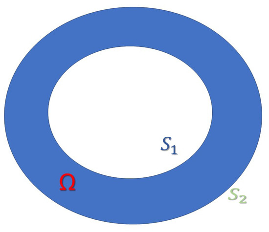
Figure 1. Bi-dimensional circular annular region $\Omega$.

We consider the following boundary value problem: Find $\omega$, such that

$$\begin{array}{c}\hfill \begin{array}{cc}\hfill \Delta w& =0, \mathrm{in} \Omega ,\hfill \\ \hfill w& =\Phi , \mathrm{on} S_2,\hfill \\ \hfill \sigma {\displaystyle \frac{\partial w}{\partial n}}& =\Psi , \mathrm{on} S_2,\hfill \end{array}\end{array}$$

(1)

where $\Phi \in {\mathrm{H}}^{1/2}\left(S_2\right),{\left.\sigma {\displaystyle \frac{\partial w}{\partial n}}\right|}_{S_2}=\Psi \in {\mathrm{H}}^{-1/2}\left(S_2\right)$, n is the outward unitary vector defined on $\partial \Omega$, and $\partial w/\partial n$ denotes the outward normal derivative of w on $S_2$. For simplicity, we consider (1) with $\Psi \equiv 0$ by the change in variable $u=w-w_1$, where $w_1$ is the unique harmonic function satisfying ${\left.\sigma \partial w_1/\partial n\right|}_{S_2}=\Psi$ on $S_2$, and ${\left.w_1\right|}_{S_1}\equiv 0$. Then,

$$\begin{array}{c}\hfill \begin{array}{cc}\hfill \sigma \Delta u& =0, \mathrm{in} \Omega ,\hfill \\ \hfill u& =V, \mathrm{on} S_2,\hfill \\ \hfill \sigma \frac{\partial u}{\partial n}& =0, \mathrm{on} S_2,\hfill \end{array}\end{array}$$

(2)

where $V=\Phi -{\left.w_1\right|}_{S_2}\in {\mathrm{H}}^{1/2}\left(S_2\right)$. For the analysis of the Cauchy problem (2), the following problem is employed (see [15]):

Given a function φ defined on$S_1$, find u such that

$$\begin{array}{c}\hfill \begin{array}{cc}\hfill \sigma \Delta u& =0, \mathrm{in} \Omega ,\hfill \\ \hfill u& =\phi , \mathrm{on} S_1,\hfill \\ \hfill \sigma {\displaystyle \frac{\partial u}{\partial n}}& =0, \mathrm{on} S_2.\hfill \end{array}\end{array}$$

(3)

This problem is well-posed, and we will call it the auxiliary problem.

The inverse problem associated with the Cauchy problem can be formulated in the following way:

Recover the potential $u=\phi$ on $S_1$ from the measurements $u=V$ on $S_2$, where u is the solution to the auxiliary problem (3).

Definition 1. 

A function $u\in V_{\phi }$ is a weak solution to the auxiliary problem (3) if

$${\int }_{\Omega }\sigma \nabla u·\nabla vd\Omega =0,\mathit{for}\mathit{all}v\in V_0,$$

(4)

where

$$V_{\phi }=\{v\in H^1(\Omega ):v=\phi on S_1\},$$

(5)

$$V_0=\{v\in H^1(\Omega ):v=0 on S_1\}.$$

(6)

Theorem 1 given in [1] guarantees the existence and uniqueness of the weak solution and allows us to define the lineal, injective, and compact operator $K:H^{m-1/2}\left(S_1\right)\to L_2\left(S_2\right)$ that associates to each $\phi \in H^{m-1/2}\left(S_1\right)$ the trace over $S_2$ of the weak solution u to the auxiliary problem (3). Operator K is compact because it is the composition of the continuous operator $T:H^{m-1/2}\left(S_1\right)\to H^1(\Omega )$, which associates to each $\phi \in H^{m-1/2}\left(S_1\right)$ the weak solution to the auxiliary problem (3), with the trace operator $Tr$ from $H^m(\Omega )$ into $L_2(\partial \Omega )$, which is compact. The relationship between problem (2) and auxiliary problem (3) can be described by the operator K as follows:

A solution to the auxiliary problem (3) is also a solution to the problem (2) if we choose ϕ on $S_1$, such that

$$\begin{array}{c}\hfill {K\phi :=u\left(\phi \right)|}_{S_2}=V,\end{array}$$

(7)

where $u\left(\phi \right)$ denotes the solution to the auxiliary problem (3), and V is the known measurement in problem (2), so we have $\phi =K^{-1}\left(V\right)$.

The following result is very important for the statement of the minimization problem presented in Section 3, and its demonstration can be found in [10].

Theorem 1. 

$Im\left(K\right)$ is dense in $L_2\left(S_2\right)$.

Equation (7) does not have a solution for all $V\in L_2\left(S_2\right)$. However, if we impose some smoothness conditions on V, we can find global conditions of the existence of the solution, as in [10]. As K is an injective and well-defined [15] operator, it ensures uniqueness when a solution is available. Since the operator K is linear, injective, and compact, its inverse $K^{-1}$ is not continuous. Therefore, the inverse problem is ill-posed due to its numerical instability.

2.2. Fractional Boundary Operator

The following material has been obtained from [24]. Let ${\Omega }_1=\{x:|x|<1\}$ be a unit ball, $2\le n$. The $\partial \Omega$ corresponds with the unit sphere; $r=\left|x\right|,\overline{x}={\displaystyle \frac{x}{r}}$, let ${\displaystyle \delta =r\frac{d}{dr}}$ be a Dirac operator, where ${\displaystyle r\frac{d}{dr}=\sum _{j=1}^n{x}_j\frac{\partial }{\partial x_j}}$. Let $u\left(x\right)$ be a smooth function on the domain $\overline{\Omega }$. For any $\alpha >0$, the following expression

$${\displaystyle J^{\beta }\left[u\right]\left(x\right)=\frac{1}{\Gamma \left(\beta \right)}{\int }_0^r{\left(ln\frac{r}{s}\right)}^{\beta -1}\frac{u\left(s\overline{x}\right)}{s}ds,x\in {\Omega }_1}$$

(8)

is called an operator of integration of the order $\beta$ in the Hadamard sense. Furthermore, we will assume that $J^0\left[u\right]\left(x\right)=u\left(x\right),x\in \Omega .$

We consider the following modification of the Hadamard operator:

$$D_m^{\beta }\left[u\right]\left(x\right)=J^{m-\beta }\left[{\delta }^{m}u\right]\left(x\right)={\displaystyle \frac{1}{\Gamma (m-\beta )}}{\int }_0^r{\left(ln{\displaystyle \frac{r}{s}}\right)}^{m-1-\beta }{\left(s{\displaystyle \frac{d}{ds}}\right)}^m{\displaystyle \frac{u\left(s\overline{x}\right)}{s}}ds,$$

(9)

where m is a positive integer.

Properties and applications of the operators $J^{\beta }$ y $D^{\beta }$ have been studied in [24]. In that paper, the authors studied a certain generalization of the classical Neumann problem with the fractional order of boundary operators. Let $0<{\beta }_n<\dots <{\beta }_1<\beta \le 1$, $P_N\left(D\right)=D_m^{\beta }+{\sum }_{j=1}^N{a}_j{D}_m^{\beta j}$. In the domain ${\Omega }_1$, the authors consider the following problem:

$$\Delta u\left(x\right)=0,x\in {\Omega }_1,$$

(10)

$$P_N\left(D\right)u\left(x\right)=f\left(x\right),x\in \partial {\Omega }_1.$$

(11)

As a solution to the last problem, the authors consider a function $u\in C^2\left({\Omega }_1\right)\cap C\left(\overline{{\Omega }_1}\right)$ satisfying Equation (10) and the boundary condition (11) in a classical sense. Since $J^0\left[u\right]\left(x\right)=u\left(x\right)$, then $D^1\left[u\right]\left(x\right){\mid }_{\partial {\Omega }_1}=r\frac{du}{dr}{\mid }_{\partial {\Omega }_1}=\frac{du}{dn}{\mid }_{\partial {\Omega }_1}$, where $n$ is a normal vector to the boundary of the domain $\Omega$. Therefore, in the case $\beta =1$ and $a_j=0,j=1,\dots ,n$, we obtain the classical Neumann problem.

2.3. Fractional Cauchy Problem

We consider the following fractional Cauchy problem

$$\begin{array}{c}\hfill \begin{array}{cc}\hfill \Delta u& =0,\mathrm{in}\Omega ,\hfill \\ \hfill {\left.D_m^{\beta }u\right|}_{S_2}& =V,\mathrm{on}{S}_2,\hfill \\ \hfill \frac{\partial u}{\partial n}& =0,\mathrm{on}{S}_2,\hfill \end{array}\end{array}$$

(12)

where the operator $D_m^{\beta }$ is given in (9).

In this case, the operator $D_m^{\beta }u\left(x\right)={\displaystyle \frac{1}{\Gamma (m-\beta )}}{\int }_{R_1}^r{\left(ln{\displaystyle \frac{r}{s}}\right)}^{m-1-\beta }{\left(s{\displaystyle \frac{d}{ds}}\right)}^m{\displaystyle \frac{u\left(s\overline{x}\right)}{s}}ds$. We note that the operator is linear and continuous, and it has no singularities since $R_1\le r,s\le R_2$. For the analysis of the fractional Cauchy problem (12), we also consider the auxiliary problem (3). We define the operator $K_m^{\beta }\left(\phi \right)=(Tr\circ \left(D_m^{\beta }T\right))\left(\phi \right)=D_m^{\beta }{u|}_{S_2}$, which is a compact operator. We have the following two definitions to study the problem that concerns us.

Definition 2. 

The Forward Problem (FP) related to the fractional Cauchy problem consists of finding the potential $V=K_m^{\beta }\left(\phi \right)$ when ϕ is known.

We can consider other fractional Cauchy problems by changing the boundary operator. We can consider different kernels for the integral operator. For example, we can take the kernel of the Riemann–Liouville and Caputo fractional derivative, which can be found in [25].

Definition 3. 

Given $V\in L_2\left(S_2\right)$, the Inverse Problem (IP) related to the fractional Cauchy problem consists of finding $\phi \in L_2\left(S_1\right)$ such that $K_m^{\beta }\left(\phi \right)=V$.

3. Methods

3.1. Tikhonov Regularization of the Fractional Cauchy Problem

To find an approximate solution $\phi \in L_2\left(S_1\right)$ of Equation (7) for $K=K_m^{\beta }$ when we have a measurement with error $V_{\delta }$, the minimization of the following Tikhonov functional is proposed in [26]:

$$J_{\alpha }\left(\phi \right):={\displaystyle \frac{1}{2}}{∥K_m^{\beta }\phi -V_{\delta }∥}_{L_2\left(S_2\right)}^2+{\displaystyle \frac{\alpha }{2}}{∥\phi ∥}^2,\forall \phi \in L_2\left(S_1\right),$$

(13)

where $\alpha$ is the Tikhonov regularization parameter, which will be chosen by the L-curve method, Morozov’s discrepancy principle, and numerical tests. The first and second Fréchet derivatives are given by (see Appendix A):

$$\begin{array}{cc}\hfill D{J}_{\alpha }\left(\phi \right)& =\left({\left(K_m^{\beta }\right)}^{\ast }{K}_m^{\beta }+\alpha I\right)\phi -{\left(K_m^{\beta }\right)}^{\ast }{V}_{\delta },\hfill \\ \hfill D^2{J}_{\alpha }\left(\phi \right)& ={\left(K_m^{\beta }\right)}^{\ast }{K}_m^{\beta }+\alpha I\hfill \end{array}$$

This least squares procedure is equivalent to solving the normal equation

$$\left({\left(K_m^{\beta }\right)}^{\ast }{K}_m^{\beta }+\alpha I\right)\phi ={\left(K_m^{\beta }\right)}^{\ast }V,$$

(14)

where ${\left(K_m^{\beta }\right)}^{\ast }$ is the adjoint operator.

According to Theorem 2.12 given in [26], the operator ${\left(K_m^{\beta }\right)}^{\ast }{K}_m^{\beta }+\alpha I$ is boundedly invertible. Given $\phi \in L_2\left(S_1\right)$, the exact solution to the auxiliary problem (3) in a circular annular region $R_1\le r\le R_2$, in polar coordinates, is given by

$$\begin{array}{c}\hfill u(r,\theta )={\phi }_0+{\displaystyle \sum _{k=1}^{\infty }}{\displaystyle \frac{{\left(R_2/R_1\right)}^{2k}}{{\left(R_2/R_1\right)}^{2k}+1}}\left\{\left[{\left({\displaystyle \frac{R_1}{R_2}}\right)}^k{\left({\displaystyle \frac{r}{R_2}}\right)}^k+{\left({\displaystyle \frac{R_1}{r}}\right)}^k\right]{\phi }_k^{1}cos\left(k\theta \right)\right.\\ \hfill \left.+\left[{\left({\displaystyle \frac{R_1}{R_2}}\right)}^k{\left({\displaystyle \frac{r}{R_2}}\right)}^k+{\left({\displaystyle \frac{R_1}{r}}\right)}^k\right]{\phi }_k^{2}sin\left(k\theta \right)\right\},\end{array}$$

(15)

where $0\le \theta <2\pi$. The values ${\phi }_0,{\phi }_k^1,{\phi }_k^2$, $k=1,2,\dots$, are the Fourier coefficients of $\phi$. The solution to the FP, called measurement, is given by $V=K_m^{\beta }\phi$, which is obtained by applying the operator $D_m^{\beta }$, the identities

${\left(s{\displaystyle \frac{d}{ds}}\right)}^m(s^{k}cos\left(k\theta \right))=k^m{s}^{k}cos\left(k\theta \right)$, ${\left(s{\displaystyle \frac{d}{ds}}\right)}^m(s^{-k}cos\left(k\theta \right))={(-1)}^m{k}^m{s}^{-k}cos\left(k\theta \right)$,

${\left(s{\displaystyle \frac{d}{ds}}\right)}^m(s^{k}sin\left(k\theta \right))=k^m{s}^{k}sin\left(k\theta \right)$, ${\left(s{\displaystyle \frac{d}{ds}}\right)}^m(s^{-k}sin\left(k\theta \right))={(-1)}^m{k}^m{s}^{-k}sin\left(k\theta \right)$, and then evaluating in $r=R_2$, i.e.,

$$\begin{array}{c}\hfill V\left(\theta \right)=K_m^{\beta }\phi \left(\theta \right)=(Tr\circ \left(D_m^{\beta }T\right))\phi \left(\theta \right)=D_m^{\beta }{u|}_{S_2}\left(\theta \right)\\ \hfill ={\displaystyle \sum _{k=1}^{\infty }}{G}_{m,k}^{\beta }({\phi }_k^{1}cos\left(k\theta \right)+{\phi }_k^{2}sin\left(k\theta \right)),\end{array}$$

(16)

where the Fourier coefficients $V_k^i$ of exact measurement V are given by $V_k^i=G_{m,k}^{\beta }{\phi }_k^i$, for $i=1$, 2, in which

$$G_{m,k}^{\beta }={\displaystyle \frac{k^m}{\Gamma (m-\beta )}}{\int }_{R_1}^{R_2}{\left(ln{\displaystyle \frac{R_2}{s}}\right)}^{m-1-\beta }\left[{\left({\displaystyle \frac{R_1}{R_2}}\right)}^k{\displaystyle \frac{s^{k-1}}{R_2^k}}+{(-1)}^m{R}_1^k{s}^{-k}\right]ds.$$

(17)

In the numerical examples, the integrals are calculated using the function quadl of MATLAB.

The ‘exact solution’ u and the ‘exact measurement’ ${V=v|}_{S_2}$ are generated taking $2N+1$ terms of the Fourier series (15) and (16), with $N=15$, which is obtained from numerical tests. To find the solution to the IP, we must solve the normal equations. To do this, we calculate the adjoint operator using its definition:

$$⟨{\left(K_m^{\beta }\right)}^{\ast }W){,\phi ⟩}_{L_2\left(S_1\right)}={⟨V,K_m^{\beta }\phi ⟩}_{L_2\left(S_2\right)}.$$

(18)

Without loss of generality, we consider functions in which the constant term of their series expansion is null. Using (16) and (18), we found

$$\begin{array}{cc}\hfill & {⟨W,K_m^{\beta }\phi ⟩}_{L_2\left(S_2\right)}=\hfill \\ \hfill & ⟨{\displaystyle \sum _{j=1}^{\infty }}{W}_j^{1}cos\left(j\theta \right)+W_j^{2}sin\left(j\theta \right),{\displaystyle \sum _{k=1}^{\infty }}{G}_{m,k}^{\beta }{\phi }_k^{1}cos\left(k\theta \right)+G_{m,k}^{\beta }{\phi }_k^{2}sin\left(k\theta \right){⟩}_{L_2\left(S_2\right)}\hfill \\ \hfill & =⟨{\displaystyle \frac{R_2}{R_1}}{\displaystyle \sum _{j=1}^{\infty }}{G}_{m,k}^{\beta }{W}_j^{1}cos\left(j\theta \right)+G_{m,k}^{\beta }{W}_j^{2}sin\left(j\theta \right),{\displaystyle \sum _{k=1}^{\infty }}{\phi }_k^{1}cos\left(k\theta \right)+{\phi }_k^{2}sin\left(k\theta \right){⟩}_{L_2\left(S_1\right)}\hfill \\ \hfill & ={⟨{\left(K_m^{\beta }\right)}^{\ast }W,\phi ⟩}_{L_2\left(S_1\right)}.\hfill \end{array}$$

(19)

Thus, the adjoint operator is defined by ${\left(K_m^{\beta }\right)}^{\ast }:L_2\left(S_2\right)\to L_2\left(S_1\right)$,

$${\left(K_m^{\beta }\right)}^{\ast }\left(W\right)={\displaystyle \frac{R_2}{R_1}}{\displaystyle \sum _{k=1}^{\infty }}{G}_{m,k}^{\beta }(W_k^{1}cos\left(k\theta \right)+W_k^{2}sin\left(k\theta \right)).$$

(20)

After some calculations, the regularized solution ${\phi }_{\alpha \left(\delta \right)}$ that minimizes the functional (13) or that solves normal Equation (14) is given by

$${\phi }_{\alpha \left(\delta \right)}\left(\theta \right)={\displaystyle \sum _{k=1}^{\infty }}\left({\phi }_{k,\alpha \left(\delta \right)}^{1}cos\left(k\theta \right)+{\phi }_{k,\alpha \left(\delta \right)}^{2}sin\left(k\theta \right)\right),\mathrm{on}{S}_1,$$

(21)

where

$$\begin{array}{c}\hfill {\phi }_{k,\alpha \left(\delta \right)}^i={\displaystyle \frac{R_2{G}_{m,k}^{\beta }}{{\left(G_{m,k}^{\beta }\right)}^2{R}_2+\alpha R_1}}{V}_{k,\delta }^i, \mathrm{for} i=1,2, \mathrm{and} k=1,2,\dots ,N,\end{array}$$

and $V_{k,\delta }^i$ are the Fourier coefficients of measurement with error $V_{\delta }$.

3.2. Tikhonov Regularization for the Classical Cauchy Problem

Given $\phi \in L_2\left(S_1\right)$, the exact solution $u(r,\theta )$ to the auxiliary problem (3) in a circular annular region $R_1\le r\le R_2$ is given, in polar coordinates, by (15). Therefore, the measurement ${V=u|}_{S_2}$ is obtained with $r=R_2$ in (15):

$$V\left(\theta \right)={\left.u(r,\theta )\right|}_{r=R_2}={\phi }_0+2{\displaystyle \sum _{k=1}^{\infty }}{\displaystyle \frac{{\left(R_2/R_1\right)}^k}{{\left(R_2/R_1\right)}^{2k}+1}}\left\{{\phi }_k^{1}cos\left(k\theta \right)+{\phi }_k^{2}sin\left(k\theta \right)\right\},$$

(22)

which is the solution to the FP. The Fourier coefficients of V are given by

$$V_0={\phi }_0 \mathrm{and}=V_k^i={\displaystyle \frac{2{\left(R_2/R_1\right)}^k}{{\left(R_2/R_1\right)}^{2k}+1}}{\phi }_k^i, \mathrm{for} i=1,2.$$

Therefore, the solution to the IP from the measurement with error

$$V_{\delta }\left(\theta \right)=V_{0,\delta }+{\displaystyle \sum _{k=1}^{\infty }}\left(V_{k,\delta }^{1}cos\left(k\theta \right)+V_{k,\delta }^{2}sin\left(k\theta \right)\right)\mathrm{on}{S}_1,$$

(23)

is given by the regularized solution

$${\phi }_{\alpha \left(\delta \right)}\left(\theta \right)={\phi }_{0,\alpha \left(\delta \right)}+{\displaystyle \sum _{k=1}^{\infty }}\left({\phi }_{k,\alpha \left(\delta \right)}^{1}cos\left(k\theta \right)+{\phi }_{k,\alpha \left(\delta \right)}^{2}sin\left(k\theta \right)\right)\mathrm{on}{S}_1,$$

(24)

where

$$\begin{array}{c}\hfill {\phi }_{k,\alpha \left(\delta \right)}^i={\displaystyle \frac{{\left(\frac{R_2}{R_1}\right)}^k\left[1+{\left(\frac{R_2}{R_1}\right)}^{2k}\right]}{2{\left(\frac{R_2}{R_1}\right)}^{2k}+\frac{\alpha R_1}{2R_2}{\left[1+{\left(\frac{R_2}{R_1}\right)}^{2k}\right]}^2}}{V}_{k,\delta }^i,i=1,2,k=1,2,3,\dots \end{array}$$

(25)

where $V_{k,\delta }^i$ are the Fourier coefficients of $V_{\delta }$ and $\alpha$ is the Tikhonov regularization parameter. Thus, the solution to the IP (of the classical Cauchy problem) applying the Tikhonov regularization method (TRM) is given by (15), replacing the coefficients ${\phi }_k^i$ by the coefficients ${\phi }_{k,\alpha \left(\delta \right)}^i$ given by (25).

4. Numerical Results

In this section, we illustrate the method proposed in this work using synthetic examples. We know the exact $\phi$ defined on $S_1$ in this case. Then, we calculated the measurement with and without noise by solving the FP for the classical and fractional Cauchy problem.

The exact measurement is calculated by solving the FP. To generate the measurements with error $V_{\delta }$, we added to the exact measurement a Gaussian error using the function $random$ of MATLAB. The exact measurement was calculated by solving the FP. Therefore, we define

$$V_{\delta }=V+E,$$

(26)

where $E=random($‘$Normal$’$,{\mu }_0,$${\sigma }_0,1,m)$ is a vector of random numbers of length m (numbers of nodes on $S_2$) with a normal distribution. The corresponding numerical solutions are denoted by ${\phi }_{\alpha \left(\delta \right)}$.

In this section, we obtain the relative error between the exact source $\phi$ and the recovered source ${\phi }_{\alpha \left(\delta \right)}$ shown in tables and denoted by $RE(\phi ,{\phi }_{\alpha \left(\delta \right)})$. The relative error is given by

$$RE(\phi ,{\phi }_{\alpha \left(\delta \right)})=\parallel \phi -{\phi }_{\alpha \left(\delta \right)}{\parallel }_{L_2\left(S_1\right)}/{\parallel \phi \parallel }_{L_2\left(S_1\right)},$$

and the relative error between the exact measurement V and the measurement with error $V_{\delta }$ is denoted by $RE(V,V_{\delta })$, which is given by

$$RE(V,V_{\delta })=\parallel V-V_{\delta }{\parallel }_{L_2\left(S_2\right)}/{\parallel V\parallel }_{L_2\left(S_2\right)},$$

where ${\parallel ·\parallel }_{L_2\left(S_i\right)}$ is the norm of the space $L_2\left(S_i\right),i=1,2$.

4.1. Solution to the IP Related to the Classical Cauchy Problem

In the following two examples, we consider a circular annular region $R_1\le r\le R_2$ with $R_1=1$ and $R_2=1.2$; then $S_1$ and $S_2$ are two circumferences of radii $R_1=1$ and $R_2=1.2$ (see Figure 1), respectively.

Example 1. 

We take the ‘exact potential’ $\phi (x,y)=x^2-y^2$, $(x,y)\in S_1$, that in polar coordinates is $\phi \left(\theta \right)=cos\left(2\theta \right)$. In this case, $V_0={\phi }_0=0$, and the solution to the forward problem, that is, the solution to the auxiliary problem (3), is given by

$$V\left(\theta \right)=K\phi \left(\theta \right)={\left.u(r,\theta )\right|}_{r=R_2}=\left[{\displaystyle \frac{2{\left(\frac{R_2}{R_1}\right)}^2}{1+{\left(\frac{R_2}{R_1}\right)}^4}}\right]{\phi }_2^{1}cos\left(2\theta \right),\theta \in [0,2\pi ],$$

where ${\phi }_2^1=1$. Then, the ‘exact solution’ V and the ‘measurement with error’ $V_{\delta }$ are generated with the first N terms of the Fourier series (22) and (23), respectively. In this case, we take values of $N=20$, 25, and 30 terms. For smooth functions in the Cauchy data, these values of N are obtained by combining numerical tests and the following ideas: $K\left(\phi \right)=V$ is approximated by a truncation $K_N\left(\phi \right)=V_N$ choosing N such that we can guarantee that ${∥V-V_N∥}_{L_2\left(S_2\right)}^2={∥K\left(\phi \right)-K_N\left(\phi \right)∥}_{L_2\left(S_2\right)}^2<{\displaystyle \frac{{\delta }^2}{4}}$, where the approximation $K_N\left(g\right)={\sum }_{k=1}^N\left[V_k^{1}cosk\theta +V_k^{2}sink\theta \right]$. From the Parseval equality and (22), where we found that the Fourier coefficients of V decay at least as $1/k^2$, we infer

$${∥V-V_N∥}_{L_2\left(S_2\right)}^2<2\pi /N<{\delta }^2/4.$$

(27)

From this, we can take $N>{\displaystyle \frac{8\pi }{{\delta }^2}}$ for obtaining the inequality. With this, we obtain an error regarding the truncation of the series expansion.

Now, the measurement error is simulated by adding a random error to each Fourier coefficient $V_k^1,V_k^2$, $k=1,2,\dots ,N$, such that ${∥V_N-V_{\delta ,N}∥}_{L_2\left(S_2\right)}^2<{\displaystyle \frac{{\delta }^2}{4}}$, which guarantees that ${∥V-V_{\delta ,N}∥}_{L_2\left(S_2\right)}\le \delta$.

For other functions, such as absolute value and the jump function, we have to choose other values of N. This is shown in Examples 3 and 4, which are included in Section 4.2.6 .

Thus, we consider synthetic examples; that is, we examine the fundamental elements of the problems studied, such as how real data are generated and the inherent error within them. In this way, we attempt to emulate the characteristics of real-world problems so that our proposal is closely aligned with providing a solution to them.

Therefore, the measurement with error $V_{\delta }$ is given by the series

$$V_{\delta }\left(\theta \right)=\sum _{k=1}^N\left(V_{k,\delta }^{1}cos\left(k\theta \right)+V_{k,\delta }^{2}sin\left(k\theta \right)\right)\mathrm{on}{S}_1,$$

(28)

where $V_{k,\delta }^i$ are the Fourier coefficients of $V_{\delta }$. The regularized solution ${\phi }_{\alpha \left(\delta \right)}$ to the inverse problem is given by the series (24) truncated to N terms. The solution without regularization ${\phi }_{\delta }$ to the IP is given by

$${\phi }_{\delta }\left(\theta \right)=\sum _{k=1}^N\left({\phi }_{k,\delta }^{1}cos\left(k\theta \right)+{\phi }_{k,\delta }^{2}sin\left(k\theta \right)\right)\mathrm{on}{S}_1,$$

(29)

where the coefficients ${\phi }_{k,\delta }^i$ are given by

$$\begin{array}{c}\hfill {\phi }_{k,\delta }^i={\displaystyle \frac{\left[1+{\left(\frac{R_2}{R_1}\right)}^{2k}\right]}{2{\left(\frac{R_2}{R_1}\right)}^k}}{V}_{k,\delta }^i,i=1,2.\end{array}$$

(30)

Remark 1. 

In all tables associated with the classical case, if $\alpha \left(\delta \right)=0$, then the solution ${\phi }_{\alpha \left(\delta \right)}$ is the solution without regularization ${\phi }_{\delta }$ given by (29), where the coefficients ${\phi }_{k,\delta }^i$ are given by (30).

Table 1 shows the numerical results for data with and without error, applying TRM to solve the IP of the classical Cauchy problem (2). In this case, we observe that the solutions with regularization ${\phi }_{\alpha \left(\delta \right)}$ have a percentage of relative errors around $10\%$, equal to the percentage of error included in the data with error $V_{\delta }$ for $\delta =0.1$. The regularization parameter was chosen as $\alpha \left(\delta \right)=\delta$ for $N=20$, 25, and 30. Also, we can see that the $RE(\phi ,{\phi }_{\alpha \left(\delta \right)})$ decreases when the error $\delta$ tends to zero, while the $RE(\phi ,{\phi }_{\delta })$ increases for each value of N. In particular, the $RE(\phi ,{\phi }_{\delta })$ increases faster when $N=30$, for $\delta =0.1$, $0.01$, and y $0.001$. In this case, the regularization parameter $\alpha \left(\delta \right)$ depends on $V_{\delta }$.

Table 1. Numerical results applying TRM to solve the IP related to the classical Cauchy problem (2), for $\phi (x,y)=x^2-y^2$, $(x,y)\in S_1$, and different values of $\delta$ and N.

$\mathit{\delta }$	N	$\mathit{\alpha }\left(\mathit{\delta }\right)$	$\mathit{RE}(\mathit{V},{\mathit{V}}_{\mathit{\delta }})$	$\mathit{RE}(\mathit{\phi },{\mathit{\phi }}_{\mathit{\alpha }\left(\mathit{\delta }\right)})$	$\mathit{RE}(\mathit{\phi },{\mathit{\phi }}_{\mathit{\delta }})$
0	20	0	0	0	0
0.1	20	0.1	0.1069	0.1465	0.8224
0.1	25	0.1	0.1034	0.1471	1.6048
0.1	30	0.1	0.1126	0.1435	3.0063
0.01	20	0.01	0.0102	0.0342	0.0663
0.01	25	0.01	0.0112	0.0360	0.2137
0.01	30	0.01	0.0114	0.0362	0.4820
0.001	20	0.001	9.0770 $\times {10}^{-4}$	0.0050	0.0057
0.001	25	0.001	8.8517 $\times {10}^{-4}$	0.0068	0.0122
0.001	30	0.001	9.5479 $\times {10}^{-4}$	0.0083	0.0354

Figure 2a,b show the graphs of the exact measurement V and with error $V_{\delta }$, the graphs of the exact potential $\phi$ and its approximations ${\phi }_{\alpha \left(\delta \right)}$ (with regularization) and ${\phi }_{\delta }$ (without regularization) taking $\alpha \left(\delta \right)=0.1$ and $N=30$, corresponding to Example 1, for $\delta =0.1$ (see Table 1). In Figure 2b, we can see the ill-posedness of the inverse problem if we do not apply regularization, where $RE(\phi ,{\phi }_{\alpha \left(\delta \right)})=0.1435$ and $RE(\phi ,{\phi }_{\delta })=3.0063$.

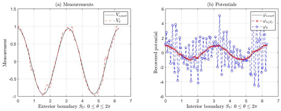
Figure 2. (a) Exact measurement V (black line) and with error $V_{\delta }$ (red line). (b) Exact potential $\phi$ and its approximations ${\phi }_{\alpha \left(\delta \right)}$ and ${\phi }_{\delta }$ applying regularization and without regularization, corresponding to Example 1 for $\delta =0.1$ (see Table 1). We take $\alpha \left(\delta \right)=0.1$ and $N=30$ in this case.

Example 2. 

We consider the ‘exact potential’ $\phi (x,y)=e^{x}sin\left(y\right)$, for $(x,y)\in S_1$. Similar to the first example, the ‘exact measurement’ V and the ‘measurement with error’ $V_{\delta }$ are generated with the first N terms of the Fourier series (22) and (23), respectively, such that $\parallel {\phi }_N{-\phi \parallel }_{L_2\left(S_1\right)}\le {ϵ}_F$, with $0<{ϵ}_F<{10}^{-14}$. In this case, $V_0={\phi }_0=0$ and the Fourier coefficients ${\phi }_k,1\le k\le N$, are obtained numerically using the intrinsic function $quadl$ of $MATLAB$. Here, we take values of $N=18$, 25, and 30 terms.

Table 2 shows the numerical results for data with and without error, applying TRM to solve the IP of the classical Cauchy problem (2). Analogous to Example 1, we can observe that the solutions with regularization ${\phi }_{\alpha \left(\delta \right)}$ have a percentage of relative errors around $10\%$, equal to the percentage of error included in the data with error $V_{\delta }$ for $\delta =0.1$. Also, we can see that the $RE(\phi ,{\phi }_{\alpha \left(\delta \right)})$ decreases when the error $\delta$ tends to zero, while the $RE(\phi ,{\phi }_{\delta })$ increases for each value of N. In particular, the $RE(\phi ,{\phi }_{\delta })$ increases when $N=30$ for each $\delta =0.1$, $0.01$, and $0.001$. As in the previous example, the regularization parameter $\alpha \left(\delta \right)$ depends on $V_{\delta }$, and we take $\alpha \left(\delta \right)=\delta$ for each value of $N=18$, 25, and 30.

Table 2. Numerical results applying TRM to solve the IP related to the classical Cauchy problem (2), for $\phi (x,y)=e^{x}sin\left(y\right)$, $(x,y)\in S_1$ and different values of $\delta$ and N.

$\mathit{\delta }$	N	$\mathit{\alpha }\left(\mathit{\delta }\right)$	$\mathit{RE}(\mathit{V},{\mathit{V}}_{\mathit{\delta }})$	$\mathit{RE}(\mathit{\phi },{\mathit{\phi }}_{\mathit{\alpha }\left(\mathit{\delta }\right)})$	$\mathit{RE}(\mathit{\phi },{\mathit{\phi }}_{\mathit{\delta }})$
0	18	0	0	2.5338 × ${10}^{-17}$	2.4537 × ${10}^{-17}$
0.1	18	0.1	0.1161	0.1590	0.8005
0.1	25	0.1	0.1125	0.1571	1.6366
0.1	30	0.1	0.1340	0.1512	5.7825
0.01	18	0.01	0.0117	0.0357	0.0509
0.01	25	0.01	0.0105	0.0392	0.1485
0.01	30	0.01	0.0112	0.0364	0.3478
0.001	18	0.001	8.8274 × ${10}^{-4}$	0.0046	0.0048
0.001	25	0.001	9.9199 × ${10}^{-4}$	0.0095	0.0162
0.001	30	0.001	0.0011	0.0099	0.0423

Figure 3a,b show the graphs of the exact measurement V and with error $V_{\delta }$, the graphs of the exact potential $\phi$ and its approximations ${\phi }_{\alpha \left(\delta \right)}$ (with regularization) and ${\phi }_{\delta }$ (without regularization) taking $\alpha \left(\delta \right)=0.1$ and $N=30$, corresponding to Example 2, for $\delta =0.1$ (see Table 2). In Figure 3b, we can see the ill-posedness of the inverse problem if we do not apply regularization. In this case, $RE(\phi ,{\phi }_{\alpha \left(\delta \right)})=0.1512$ and $RE(\phi ,{\phi }_{\delta })=5.7825$.

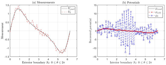
Figure 3. (a) Exact measurement V (black line) and with error $V_{\delta }$ (red line). (b) Exact potential $\phi$ and its approximations ${\phi }_{\alpha \left(\delta \right)}$ and ${\phi }_{\delta }$ applying regularization and without regularization, corresponding to Example 2 for $\delta =0.1$ (see Table 2). In this case, we take $\alpha \left(\delta \right)=0.1$ and $N=30$.

4.2. Solution to the IP Related to the Fractional Cauchy Problem

In this section, we look into the performance of the TRM to solve the IP of the fractional Cauchy problem (12) in a circular annular region $R_1\le r\le R_2$ with $R_1=1$ and $R_2=1.2$. Then, $S_1$ and $S_2$ are two circumferences of radii $R_1=1$ and $R_2=1.2$ (see Figure 1), respectively. In this case, we consider as ‘exact potentials’ the two functions from the previous subsection: $\phi (x,y)=x^2-y^2$ and $\phi (x,y)=e^{x}sin\left(y\right)$, for $(x,y)\in S_1$.

Similar to the previous subsection, the ‘exact solution’ V and the ‘measurement with error’ $V_{\delta }$ are obtained by truncating the series (16) and (23) up to N terms, respectively; furthermore, the Fourier coefficients ${\phi }_k^1$, ${\phi }_k^2$, and $G_{m,k}^{\beta }$ (given by (17)) are obtained numerically using the function $quadl$ of $MATLAB$.

In this case, we take values of $N=18$, 20, 25, and 30 terms. Therefore, the measurement with error $V_{\delta }$ is given by the series (23) truncated to N terms. The regularized solution ${\phi }_{\alpha \left(\delta \right)}$ to the IP is given by the series (21) truncated to N terms. Also, the solution without regularization ${\phi }_{\delta }$ to the IP is given by (29), where

$$\begin{array}{c}\hfill {\phi }_{k,\delta }^i={\displaystyle \frac{1}{G_{m,k}^{\beta }}}{V}_{k,\delta }^i,i=1,2,k=1,2,\dots ,N.\end{array}$$

(31)

Remark 2. 

In all tables from the fractional case, if $\alpha \left(\delta \right)=0$, the solution ${\phi }_{\alpha \left(\delta \right)}$ is the solution without regularization ${\phi }_{\delta }$ given by (29), where the coefficients ${\phi }_{k,\delta }^i$ are given by (31).

4.2.1. Case 1: $\beta =0.5$ and $m=1$, When $\delta$ Tends to Zero

In this section, we consider the case when $\beta =0.5$, $m=1$, and for different values of $\delta$ close to zero. Table 3 and Table 4 show the relative errors of the approximations ${\phi }_{\alpha \left(\delta \right)}$ and ${\phi }_{\delta }$, when $\delta$ tends to zero, for the two exact functions $\phi$ considered in Section 4.1. In both cases, we observe that the $RE(\phi ,{\phi }_{\alpha \left(\delta \right)})$ of the solutions with regularization ${\phi }_{\alpha \left(\delta \right)}$ is less than the $RE(V,V_{\delta })$ for each value of $\delta$ and N given in these tables. Additionally, the $RE(\phi ,{\phi }_{\alpha \left(\delta \right)})$ and $RE(\phi ,{\phi }_{\delta })$ are of the same order, i.e., the solutions without regularization ${\phi }_{\delta }$ are close to regularized solutions ${\phi }_{\alpha \left(\delta \right)}$ for $\beta =0.5$ and $m=1$. In both cases, the measurements with errors $V_{\delta }$ do not have much impact on recovered solution ${\phi }_{\delta }$, and they are close to ${\phi }_{\alpha \left(\delta \right)}$. We observe from the relative errors that regularized approximations ${\phi }_{\alpha \left(\delta \right)}$ are better than those without regularization. In this case, the regularization parameter $\alpha \left(\delta \right)$ depends on $V_{\delta }$, N, m, and $\beta$.

Table 3. Numerical results applying TRM to solve IP related to the fractional Cauchy problem (12), for $\phi (x,y)=x^2-y^2$, $(x,y)\in S_1$, and different values of $\delta$ and N.

$\mathit{\delta }$	N	$\mathit{\alpha }\left(\mathit{\delta }\right)$	$\mathit{\beta }$	m	$\mathit{RE}(\mathit{V},{\mathit{V}}_{\mathit{\delta }})$	$\mathit{RE}(\mathit{\phi },{\mathit{\phi }}_{\mathit{\alpha }\left(\mathit{\delta }\right)})$	$\mathit{RE}(\mathit{\phi },{\mathit{\phi }}_{\mathit{\delta }})$
0	20	0	0.5	1	0	1.1102 × ${10}^{-16}$	0
0.1	20	1 × ${10}^{-2}$	0.5	1	0.0970	0.0617	0.0880
0.1	25	1 × ${10}^{-2}$	0.5	1	0.0979	0.0719	0.0990
0.1	30	1 × ${10}^{-2}$	0.5	1	0.1038	0.0775	0.1217
0.01	20	1 × ${10}^{-4}$	0.5	1	0.0093	0.0037	0.0039
0.01	25	1 × ${10}^{-4}$	0.5	1	0.0091	0.0070	0.0070
0.01	30	1 × ${10}^{-4}$	0.5	1	0.0127	0.0072	0.0073
0.001	20	1 × ${10}^{-6}$	0.5	1	9.6950 × ${10}^{-4}$	8.9805 × ${10}^{-4}$	8.9826 × ${10}^{-4}$
0.001	25	1 × ${10}^{-6}$	0.5	1	8.3006 × ${10}^{-4}$	3.4557 × ${10}^{-4}$	3.4620 × ${10}^{-4}$
0.001	30	1 × ${10}^{-6}$	0.5	1	9.8327 × ${10}^{-4}$	5.4898 × ${10}^{-4}$	5.4925 × ${10}^{-4}$

Table 4. Numerical results applying TRM to solve IP related to the fractional Cauchy problem (12), for $\phi (x,y)=e^{x}sin\left(y\right)$, $(x,y)\in S_1$, and different values of $\delta$ and N.

$\mathit{\delta }$	N	$\mathit{\alpha }\left(\mathit{\delta }\right)$	$\mathit{\beta }$	m	$\mathit{RE}(\mathit{V},{\mathit{V}}_{\mathit{\delta }})$	$\mathit{RE}(\mathit{\phi },{\mathit{\phi }}_{\mathit{\alpha }\left(\mathit{\delta }\right)})$	$\mathit{RE}(\mathit{\phi },{\mathit{\phi }}_{\mathit{\delta }})$
0	18	0	0.5	1	0	2.4537 × ${10}^{-17}$	2.4537 × ${10}^{-17}$
0.1	18	1 × ${10}^{-4}$	0.5	1	0.1292	0.1196	0.1212
0.1	25	1 × ${10}^{-4}$	0.5	1	0.1732	0.1238	0.1296
0.1	30	1 × ${10}^{-4}$	0.5	1	0.1921	0.0624	0.0672
0.01	18	1 × ${10}^{-5}$	0.5	1	0.0147	0.0126	0.0129
0.01	25	1 × ${10}^{-5}$	0.5	1	0.0166	0.0124	0.0129
0.01	30	1 × ${10}^{-5}$	0.5	1	0.0177	0.0069	0.0071
0.001	18	1 × ${10}^{-6}$	0.5	1	0.0012	8.6623 × ${10}^{-4}$	9.1811 × ${10}^{-4}$
0.001	25	1 × ${10}^{-6}$	0.5	1	0.0017	8.6801 × ${10}^{-4}$	9.1904 × ${10}^{-4}$
0.001	25	1 × ${10}^{-6}$	0.5	1	0.0018	7.3211 × ${10}^{-4}$	7.7961 × ${10}^{-4}$

Considering $\delta =0.1$, $\beta =0.5$, and $m=1$, we show the graphs for the following potentials $\phi (x,y)=x^2-y^2$ (Figure 4) and $\phi (x,y)=e^{x}sin\left(y\right)$ (Figure 5) for $(x,y)\in S_1$ where the following is true:

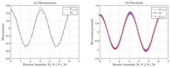
Figure 4. (a) Exact measurement V (black line) and with error $V_{\delta }$ (red line). (b) Exact potential $\phi$ and its approximations ${\phi }_{\alpha \left(\delta \right)}$ and ${\phi }_{\delta }$, corresponding to Example 1 for $\delta =0.1$ (see Table 3). In this case, we take $\alpha \left(\delta \right)={10}^{-2}$ and $N=30$.

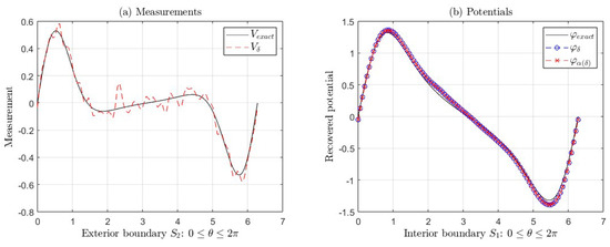
Figure 5. (a) Exact measurement V (black line) and with error $V_{\delta }$ (red line). (b) Exact potential $\phi$ and its approximations ${\phi }_{\alpha \left(\delta \right)}$ and ${\phi }_{\delta }$, corresponding to Example 2 for $\delta =0.1$ (see Table 4). In this case, we take $\alpha \left(\delta \right)={10}^{-4}$ and $N=30$.

(a)

The exact measurement V and the measurement with error $V_{\delta }$.

(b)

The exact potential $\phi$ and its approximations ${\phi }_{\alpha \left(\delta \right)}$ (with regularization) and ${\phi }_{\delta }$ (without regularization) taking $\alpha \left(\delta \right)={10}^{-2}$ and $N=30$.

See Table 3 and Table 4 for other values of the parameters N and $\delta$.

In Figure 4b, the $RE(\phi ,{\phi }_{\alpha \left(\delta \right)})=0.0775$ is less than $RE(\phi ,{\phi }_{\delta })=0.1217$ for $\delta =0.1$ (see Table 3). In Figure 5b, the $RE(\phi ,{\phi }_{\alpha \left(\delta \right)})=0.0624$ is less than $RE(\phi ,{\phi }_{\delta })=0.0672$ for $\delta =0.1$ (see Table 4).

4.2.2. Case 2: $\beta \in (m-1,m)$, for $m=2,\dots ,12$ and $\delta =0.1$

Table 5 and Table 6 show the relative errors of the approximations ${\phi }_{\alpha \left(\delta \right)}$ and ${\phi }_{\delta }$ when $\delta =0.1$ for the two exact functions $\phi$ considered in Section 4.1.

Table 5. Case 2: Numerical results applying TRM to solve IP related to the fractional Cauchy problem (12) for $\delta =0.1$ and different values of $\beta$ and m, where $\phi (x,y)=x^2-y^2$, $(x,y)\in S_1$.

N	$\mathit{\alpha }\left(\mathit{\delta }\right)$	$\mathit{\beta }$	m	$\mathit{RE}(\mathit{V},{\mathit{V}}_{\mathit{\delta }})$	$\mathit{RE}(\mathit{\phi },{\mathit{\phi }}_{\mathit{\alpha }\left(\mathit{\delta }\right)})$	$\mathit{RE}(\mathit{\phi },{\mathit{\phi }}_{\mathit{\delta }})$
20	1 × ${10}^{-1}$	1.5	2	0.1027	0.0360	0.0392
25	8 × ${10}^{-1}$	1.5	2	0.1017	0.0518	0.0819
30	5 × ${10}^{-1}$	1.5	2	0.1136	0.0597	0.0718
20	2 × ${10}^{-1}$	2.5	3	0.0936	0.0508	0.4857
20	1 × ${10}^1$	3.5	4	0.0969	0.0474	0.3523
20	1 × ${10}^0$	4.5	5	0.0915	0.0421	1.5924
20	1 × ${10}^2$	5.5	6	0.1112	0.0248	1.2606
20	1 × ${10}^1$	6.5	7	0.1078	0.0366	5.8758
20	1 × ${10}^2$	7.5	8	0.1045	0.0351	2.2946
20	1 × ${10}^2$	8.5	9	0.0916	0.0197	16.6149
20	1 × ${10}^3$	9.5	10	0.0996	0.0274	21.0258
20	1 × ${10}^3$	10.5	11	0.0939	0.0176	46.6720
20	1 × ${10}^3$	11.5	12	0.0861	0.0407	33.8060

Table 6. Case 2: Numerical results applying TRM to solve IP related to the fractional Cauchy problem (12) for $\delta =0.1$ and different values of $\beta$ and m, where $\phi (x,y)=e^{x}sin\left(y\right)$, $(x,y)\in S_1$.

N	$\mathit{\alpha }\left(\mathit{\delta }\right)$	$\mathit{\beta }$	m	$\mathit{RE}(\mathit{V},{\mathit{V}}_{\mathit{\delta }})$	$\mathit{RE}(\mathit{\phi },{\mathit{\phi }}_{\mathit{\alpha }\left(\mathit{\delta }\right)})$	$\mathit{RE}(\mathit{\phi },{\mathit{\phi }}_{\mathit{\delta }})$
18	1 × ${10}^{-2}$	1.5	2	0.1279	0.0342	0.0411
25	1 × ${10}^{-2}$	1.5	2	0.1780	0.0258	0.0264
30	1 × ${10}^{-2}$	1.5	2	0.1732	0.0439	0.0509
18	9 × ${10}^{-4}$	2.5	3	0.1629	0.1437	0.1504
18	4 × ${10}^{-1}$	3.5	4	0.1461	0.0931	0.3543
18	1.4 × ${10}^{-1}$	4.5	5	0.1466	0.1385	7.4132
18	1 × ${10}^1$	5.5	6	0.1757	0.3306	9.1616
18	1 × ${10}^1$	6.5	7	0.1512	0.3654	478.6290
18	4.2 × ${10}^2$	7.5	8	0.1643	0.3822	310.6255
18	3 × ${10}^5$	8.5	9	0.1732	0.8982	633.1135
18	2 × ${10}^7$	9.5	10	0.2062	0.9546	4.0208 × ${10}^3$
18	2 × ${10}^7$	10.5	11	0.1712	0.8948	1.9672 × ${10}^5$
18	8 × ${10}^8$	11.5	12	0.1636	0.9326	2.2607 × ${10}^5$

In Table 5, we observe that $RE(\phi ,{\phi }_{\alpha \left(\delta \right)})<RE(V,V_{\delta })$ for each value of N, $\beta$, and m given in the mentioned table. Also, the $RE(\phi ,{\phi }_{\alpha \left(\delta \right)})$ and $RE(\phi ,{\phi }_{\delta })$ are of the same order, i.e., the solutions without regularization ${\phi }_{\delta }$ are close to regularized solutions ${\phi }_{\alpha \left(\delta \right)}$, for $\delta =0.1$, $N=20$, 25, 30, $\beta =1.5$, and $m=2$. We can see similar results in Table 6 for $\delta =0.1$, $N=18$, 25, 30, $\beta =1.5$, $2.5$, $m=2$, and 3; however the regularized approximates ${\phi }_{\alpha \left(\delta \right)}$ are better than the solutions without regularization. Furthermore, $RE(\phi ,{\phi }_{\delta })<RE(V,V_{\delta })$ and these increase suddenly, starting at $m=3$ and $m=4$ (see Table 5 and Table 6) for the functions $\phi (x,y)=x^2-y^2$ and $\phi (x,y)=e^{x}sin\left(y\right)$ for $(x,y)\in S_1$, respectively. As in the previous case, the regularization parameter $\alpha \left(\delta \right)$ changes depending on $V_{\delta }$, N, m, and $\beta$.

We show the graphs for the following functions:

•

$\phi (x,y)=x^2-y^2$ (Figure 6 with parameters $\beta =1.5$, $m=2$, $\delta =0.1$, $\alpha \left(\delta \right)=5\times {10}^{-1}$, and $N=30$; and Figure 7 with parameters $\beta =2.5$, $m=3$, $\delta =0.1$, $\alpha \left(\delta \right)=2\times {10}^{-1}$, and $N=20$).

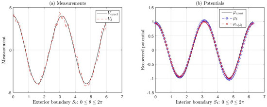Figure 6. (a) Exact measurement V (black line) and with error $V_{\delta }$ (red line). (b) Exact potential $\phi$ and its approximations ${\phi }_{\alpha \left(\delta \right)}$ and ${\phi }_{\delta }$, corresponding to Example 1 for $\beta =1.5$, $m=2$, and $\delta =0.1$ (see Table 5). In this case, we take $\alpha \left(\delta \right)=5\times {10}^{-1}$ and $N=30$.

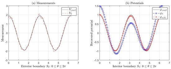Figure 7. (a) Exact measurement V (black line) and with error $V_{\delta }$ (red line). (b) Exact potential $\phi$ and its approximations ${\phi }_{\alpha \left(\delta \right)}$ and ${\phi }_{\delta }$, corresponding to Example 1 for $\beta =2.5$, $m=3$, and $\delta =0.1$ (see Table 5). In this case, we take $\alpha \left(\delta \right)=2\times {10}^{-1}$ and $N=20$.

•

$\phi (x,y)=e^{x}sin\left(y\right)$ (Figure 8 with parameters $\beta =7.5$, $m=8$, $\delta =0.1$, $\alpha \left(\delta \right)=4.2\times {10}^2$, and $N=18$).

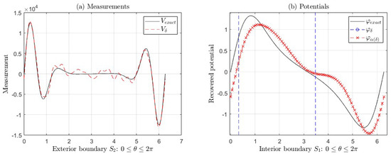Figure 8. (a) Exact measurement V (black line) and with error $V_{\delta }$ (red line). (b) Exact potential $\phi$ and its approximations ${\phi }_{\alpha \left(\delta \right)}$ and ${\phi }_{\delta }$, corresponding to Example 2 for $\beta =7.5$, $m=8$, and $\delta =0.1$ (see Table 6). In this case, we take $\alpha \left(\delta \right)=4.2\times {10}^2$ and $N=18$.

For $(x,y)\in S_1$. These figures show the following:

(a)

The exact measurement V and the measurement with error $V_{\delta }$.

(b)

The exact potential $\phi$ and its approximations ${\phi }_{\alpha \left(\delta \right)}$ (with regularization) and ${\phi }_{\delta }$ (without regularization).

In both cases, as mentioned in the previous paragraph, the errors increase suddenly, starting at $m=3$ for the first function and $m=4$ for the second one, as can be seen in Figure 7b and Figure 8b, where we can see the ill-posedness of the IP if we do not apply regularization. For example, for the second function, the $RE(\phi ,{\phi }_{\alpha \left(\delta \right)})=310.6255$ is much greater than $RE(\phi ,{\phi }_{\delta })=0.3822$ for $\beta =7.5$, $m=8$, and $\delta =0.1$ (see Table 6). However, in this same example, for $m=9$, 10, 11, and 12, the $RE(\phi ,{\phi }_{\alpha \left(\delta \right)})$ increases around 90%. Nevertheless, $RE(\phi ,{\phi }_{\delta })$ is bigger than $RE(\phi ,{\phi }_{\alpha \left(\delta \right)})$. In this case, we could use the regularized solution as an initial point of an iterative method to recover a better solution to the IP.

4.2.3. Case 3: $\beta \in (m-1,m)$, When $\beta$ Is Next to $m-1$ or m and $\delta =0.1$

This section considers the case when $m-1<\beta <m$ and $\beta$ is next to $m-1$ or m. Table 7 and Table 8 show the relative errors of the approximations ${\phi }_{\alpha \left(\delta \right)}$ and ${\phi }_{\delta }$ when $\delta =0.1$ for the same two exact functions $\phi$ considered in Section 4.1.

Table 7. Case 3: Numerical results applying TRM to solve the IP related to the fractional Cauchy problem (12) for $\delta =0.1$ and different values of $\beta$ and m, where $\phi (x,y)=x^2-y^2$, $(x,y)\in S_1$.

N	$\mathit{\alpha }\left(\mathit{\delta }\right)$	$\mathit{\beta }$	m	$\mathit{RE}(\mathit{V},{\mathit{V}}_{\mathit{\delta }})$	$\mathit{RE}(\mathit{\phi },{\mathit{\phi }}_{\mathit{\alpha }\left(\mathit{\delta }\right)})$	$\mathit{RE}(\mathit{\phi },{\mathit{\phi }}_{\mathit{\delta }})$
20	1 × ${10}^{-3}$	0.1	1	0.1093	0.0565	0.0765
20	1 × ${10}^{-5}$	0.0001	1	0.1032	0.0699	0.0705
20	1 × ${10}^{-12}$	0.0000001	1	0.1040	0.0394	0.0394
20	1 × ${10}^{-3}$	0.9	1	0.0922	0.0809	0.0817
20	1 × ${10}^{-8}$	0.9999	1	0.0988	0.0581	0.0583
20	1 × ${10}^{-12}$	0.9999999	1	0.0967	0.0921	0.1277
20	1 × ${10}^{-1}$	1.1	2	0.1081	0.0563	0.0647
20	5 × ${10}^{-2}$	1.0001	2	0.0931	0.0791	0.0984
20	1 × ${10}^{-2}$	1.0000001	2	0.0979	0.0901	0.0953
20	1 × ${10}^{-1}$	1.9	2	0.0980	0.0726	0.0746
20	1 × ${10}^{-5}$	1.9999	2	0.0971	0.0449	0.0488
20	1 × ${10}^{-11}$	1.9999999	2	0.1033	0.0997	0.1105
20	1 × ${10}^{-2}$	2.1	3	0.0998	0.0392	0.2108
20	1 × ${10}^{-2}$	2.0001	3	0.0905	0.0479	0.3250
20	1 × ${10}^{-2}$	2.0000001	3	0.0894	0.0264	0.1021
20	1 × ${10}^{-1}$	2.9	3	0.1110	0.0860	0.1731
20	1 × ${10}^{-5}$	2.9999	3	0.0999	0.0804	0.4756
20	1 × ${10}^{-11}$	2.9999999	3	0.1027	0.0672	0.3546
20	1 × ${10}^0$	3.1	4	0.1061	0.0328	0.1583
20	1 × ${10}^2$	3.9	4	0.1061	0.0738	0.5624
20	1 × ${10}^{-1}$	4.1	5	0.0863	0.0421	1.8856
20	1 × ${10}^0$	4.9	5	0.1030	0.0401	0.2528
20	1 × ${10}^1$	5.1	6	0.0751	0.0368	1.5197
20	1 × ${10}^2$	5.9	6	0.0957	0.0438	1.0323
20	1 × ${10}^0$	6.1	7	0.0917	0.0267	5.3155
20	1 × ${10}^0$	6.9	7	0.1020	0.0600	5.5627
20	1 × ${10}^2$	7.1	8	0.0935	0.0199	3.3483
20	1 × ${10}^2$	7.0000001	8	0.0827	0.0206	1.7258
20	1 × ${10}^3$	7.9	8	0.0870	0.0212	4.5019
20	1 × ${10}^{-8}$	7.9999999	8	0.0986	0.0454	4.2454
20	1 × ${10}^1$	8.1	9	0.1155	0.0276	14.3075
20	1 × ${10}^2$	8.9	9	0.0953	0.0342	34.0155
20	1 × ${10}^2$	9.1	10	0.1013	0.0508	20.6047
20	1 × ${10}^4$	9.9	10	0.0972	0.0095	24.1306
20	1 × ${10}^2$	10.1	11	0.0941	0.0271	35.0730
20	1 × ${10}^3$	10.9	11	0.0956	0.0090	90.0697
20	1 × ${10}^3$	11.1	12	0.0951	0.0226	65.9229
20	1 × ${10}^4$	11.9	12	0.0967	0.0475	101.7022

Table 8. Case 3: Numerical results applying TRM to solve IP related to the fractional Cauchy problem (12) for $\delta =0.1$ and different values of $\beta$ and m, where $\phi (x,y)=e^{x}sin\left(y\right)$, $(x,y)\in S_1$.

N	$\mathit{\alpha }\left(\mathit{\delta }\right)$	$\mathit{\beta }$	m	$\mathit{RE}(\mathit{V},{\mathit{V}}_{\mathit{\delta }})$	δ$\mathit{RE}(\mathit{\phi },{\mathit{\phi }}_{\mathit{\alpha }\left(\mathit{\delta }\right)})$	$\mathit{RE}(\mathit{\phi },{\mathit{\phi }}_{\mathit{\delta }})$
30	1 × ${10}^{-5}$	0.1	1	0.1429	0.0210	0.0230
30	1 × ${10}^{-6}$	0.0001	1	0.1849	0.0396	0.0401
30	1 × ${10}^{-13}$	0.0000001	1	0.1762	0.0314	0.0314
30	1 × ${10}^{-4}$	0.9	1	0.1674	0.0448	0.0452
30	1 × ${10}^{-8}$	0.9999	1	0.1299	0.0544	0.0575
30	1 × ${10}^{-15}$	0.9999999	1	0.1748	0.0271	0.0272
30	1 × ${10}^{-5}$	1.1	2	0.1613	0.0454	0.0454
30	1 × ${10}^{-5}$	1.0001	2	0.1829	0.0492	0.0493
30	1 × ${10}^{-5}$	1.0000001	2	0.1842	0.0584	0.0585
30	1 × ${10}^{-1}$	1.9	2	0.1739	0.0353	0.0431
30	1 × ${10}^{-6}$	1.9999	2	0.1870	0.0380	0.0413
30	1 × ${10}^{-12}$	1.9999999	2	0.1690	0.0609	0.0674
30	1 × ${10}^{-4}$	2.1	3	0.2071	0.0760	0.1016
30	1 × ${10}^{-8}$	2.0001	3	0.2114	0.1688	0.1689
30	1 × ${10}^{-9}$	2.0000001	3	0.1877	0.1176	0.1176
30	3 × ${10}^{-2}$	2.9	3	0.2256	0.1156	0.2868
30	1 × ${10}^{-6}$	2.9999	3	0.1676	0.0761	0.4059
30	5 × ${10}^{-13}$	2.9999999	3	0.2155	0.1581	0.1751
30	5 × ${10}^{-2}$	3.1	4	0.2057	0.1258	0.1717
30	1 × ${10}^0$	3.9	4	0.2001	0.0881	0.3453
30	5 × ${10}^{-2}$	4.1	5	0.2545	0.3090	16.5294
30	1 × ${10}^0$	4.9	5	0.2011	0.2408	6.8619
30	4 × ${10}^0$	5.1	6	0.1983	0.4226	12.4482
30	5 × ${10}^1$	5.9	6	0.2049	0.3878	7.9340
30	7 × ${10}^{-1}$	6.1	7	0.2124	0.4678	243.7232
30	6 × ${10}^1$	6.9	7	0.2553	0.5497	363.0725
30	4 × ${10}^1$	7.1	8	0.2463	0.4505	123.0513
30	5 × ${10}^1$	7.0001	8	0.2452	0.2910	240.1527
30	2 × ${10}^1$	7.0000001	8	0.2335	0.1839	119.2328
30	2 × ${10}^3$	7.9	8	0.2184	0.1710	402.7594
30	1.3 × ${10}^{-2}$	7.9999	8	0.2308	0.3440	181.8997
30	2 × ${10}^{-8}$	7.9999999	8	0.1833	0.5806	164.4764
30	3 × ${10}^4$	8.1	9	0.2548	0.8971	3.4981 × ${10}^3$
30	2 × ${10}^6$	8.9	9	0.2054	0.9059	2.8978 × ${10}^3$
30	2 × ${10}^6$	9.1	10	0.2260	0.8857	6.8133 × ${10}^3$
30	7 × ${10}^7$	9.9	10	0.2241	0.8896	6.2431 × ${10}^3$
30	4 × ${10}^6$	10.1	11	0.2233	0.9011	2.5172 × ${10}^5$
30	2 × ${10}^8$	10.9	11	0.2069	0.8934	1.9773 × ${10}^5$
30	5 × ${10}^8$	11.1	12	0.2479	0.9212	1.1346 × ${10}^5$
30	5 × ${10}^9$	11.9	12	0.2372	0.8996	3.4904 × ${10}^5$

In Table 7, we observe that the $RE(\phi ,{\phi }_{\alpha \left(\delta \right)})$ are less than the $RE(V,V_{\delta })$ for each value of N, $\beta$, and m given in this table. We can see that $RE(\phi ,{\phi }_{\alpha \left(\delta \right)})$ and $RE(\phi ,{\phi }_{\delta })$ are of the same order for $m=1$, 2, i.e., the solutions without regularization ${\phi }_{\delta }$ are close to regularized solutions ${\phi }_{\alpha \left(\delta \right)}$. However, the regularized approximates ${\phi }_{\alpha \left(\delta \right)}$ are better than the solutions without regularization for $m=1$, 2. Nonetheless, $RE(\phi ,{\phi }_{\alpha \left(\delta \right)})$ increases more than $RE(V,V_{\delta })$ starting at $m=3$. Furthermore, we can observe similar results in Table 8, where the $RE(\phi ,{\phi }_{\alpha \left(\delta \right)})$ are less than the $RE(V,V_{\delta })$ for $m=1$, 2, 3, 4, with $\delta =0.1$, $N=30$, and the different values of $\beta$ are close to m or $m-1$ given in this table. For the values of $m=5$, 6, 7, and 8, the $RE(\phi ,{\phi }_{\alpha \left(\delta \right)})$ are around the percentage of the $RE(V,V_{\delta })$. For the other values of $m=9$, 10, 11, and 12, given in Table 8, the corresponding $RE(\phi ,{\phi }_{\alpha \left(\delta \right)})$ increases around 90%, but no more than $RE(\phi ,{\phi }_{\delta })$, i.e., the TRM does not provide a good approximate solution to the IP. In this case, we could use the regularized solution ${\phi }_{\alpha \left(\delta \right)}$ as an initial point of an iterative method to recover a better solution to the IP. Furthermore, the relative errors of the recovered solutions ${\phi }_{\delta }$ without applying regularization increase suddenly, starting at $m=7$ and $m=5$ (see Table 7 and Table 8) for the functions $\phi (x,y)=x^2-y^2$ and $\phi (x,y)=e^{x}sin\left(y\right)$ for $(x,y)\in S_1$, respectively. As in the previous cases, the regularization parameter $\alpha \left(\delta \right)$ changes depending on $V_{\delta }$, N, m, and $\beta$.

We show the graphs for the following functions:

•

$\phi (x,y)=x^2-y^2$ (Figure 9 with parameters $\beta =7.1$, $m=8$, $\delta =0.1$, $\alpha \left(\delta \right)={10}^2$, and $N=20$).

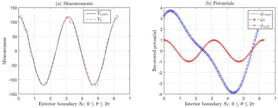Figure 9. (a) Exact measurement V (black line) and with error $V_{\delta }$ (red line). (b) Exact potential $\phi$ and its approximations ${\phi }_{\alpha \left(\delta \right)}$ and ${\phi }_{\delta }$, corresponding to Example 1 for $\beta =7.1$, $m=8$, and $\delta =0.1$ (see Table 7). In this case, we take $\alpha \left(\delta \right)={10}^2$ and $N=20$.

•

$\phi (x,y)=e^{x}sin\left(y\right)$ (Figure 10 with parameters $\beta =7.9999999$, $m=8$, $\delta =0.1$, $\alpha \left(\delta \right)=2\times {10}^{-8}$, and $N=30$).

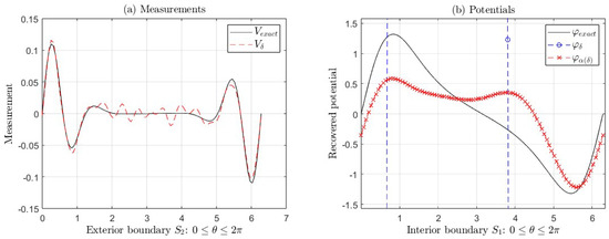Figure 10. (a) Exact measurement V (black line) and with error $V_{\delta }$ (red line). (b) Exact potential $\phi$ and its approximations ${\phi }_{\alpha \left(\delta \right)}$ and ${\phi }_{\delta }$, corresponding to Example 1 for $\beta =7.9999999$, $m=8$, and $\delta =0.1$ (see Table 8). In this case, we take $\alpha \left(\delta \right)=2\times {10}^{-8}$ and $N=30$.

For $(x,y)\in S_1$. These figures show the following:

(a)

The exact measurement V and the measurement with error $V_{\delta }$.

(b)

The exact potential $\phi$ and its approximations ${\phi }_{\alpha \left(\delta \right)}$ (with regularization) and ${\phi }_{\delta }$ (without regularization).

In both cases, as mentioned in the previous paragraph, the errors increase starting at $m=7$ for the first function and starting at $m=5$ for the second one, as can be seen in Figure 9b and Figure 10b for $m=8$, where we can see the ill-posedness of the IP if we do not apply regularization. For example, for the first function, the $RE(\phi ,{\phi }_{\delta })=3.3483$ is greater than $RE(\phi ,{\phi }_{\alpha \left(\delta \right)})=0.0199$ for $\beta =7.1$, $m=8$, and $\delta =0.1$ (see Table 7). For the second one, the $RE(\phi ,{\phi }_{\delta })=164.4764$ is greater than $RE(\phi ,{\phi }_{\alpha \left(\delta \right)})=0.5806$ for $\beta =7.9999999$, $m=8$, and $\delta =0.1$ (see Table 8). In this latter function, the approximate solution ${\phi }_{\alpha \left(\delta \right)}$ is far from the exact solution $\phi$. In this case, we could apply an iterative method to obtain a better solution, taking ${\phi }_{\alpha \left(\delta \right)}$ as an initial point.

4.2.4. Case 4: $\beta <m-1$, for $m=2$,…,12 and $\delta =0.1$

In this Section, we consider the case when $\beta <m-1$ for $m=2$, 3,…,12 and $\delta =0.1$. Table 9 and Table 10 show the relative errors of the approximations ${\phi }_{\alpha \left(\delta \right)}$ and ${\phi }_{\delta }$ when $\delta =0.1$, with the same two exact functions $\phi$ considered in the Section 4.1.

Table 9. Case 4: Numerical results applying TRM to solve the IP related to the fractional Cauchy problem (12) for $\delta =0.1$ and different values of $\beta$ and m, where $\phi (x,y)=x^2-y^2$, $(x,y)\in S_1$.

N	$\mathit{\alpha }\left(\mathit{\delta }\right)$	$\mathit{\beta }$	m	$\mathit{RE}(\mathit{V},{\mathit{V}}_{\mathit{\delta }})$	$\mathit{RE}(\mathit{\phi },{\mathit{\phi }}_{\mathit{\alpha }\left(\mathit{\delta }\right)})$	$\mathit{RE}(\mathit{\phi },{\mathit{\phi }}_{\mathit{\delta }})$
20	1 × ${10}^{-4}$	0.5	2	0.1037	0.0369	0.0371
25	1 × ${10}^{-4}$	0.5	2	0.1043	0.0846	0.0850
30	1 × ${10}^{-4}$	0.5	2	0.1123	0.0947	0.0952
20	1 × ${10}^{-7}$	0.1	3	0.0953	0.0558	0.3293
20	1 × ${10}^{-5}$	0.8	3	0.0928	0.0397	0.1176
20	1 × ${10}^{-3}$	1.6	4	0.1031	0.0692	0.3781
20	1 × ${10}^0$	2.9	4	0.0988	0.0550	0.2616
20	1 × ${10}^{-10}$	0.5	5	0.1063	0.0493	2.3272
20	1 × ${10}^{-2}$	3.5	5	0.1002	0.0479	0.6521
20	1 × ${10}^{-10}$	0.5	6	0.0824	0.0664	1.0640
20	1 × ${10}^{-3}$	3.4	6	0.1156	0.0541	1.0860
20	1 × ${10}^{-16}$	0.5	7	0.1093	0.0251	11.3550
20	1 × ${10}^{-5}$	4.2	7	0.0871	0.0203	4.0183
20	1 × ${10}^{-16}$	0.5	8	0.0915	0.0280	3.7583
20	1 × ${10}^{-6}$	3.7	8	0.1097	0.0212	4.3335
20	1 × ${10}^{-22}$	0.5	9	0.0969	0.0195	21.9486
20	1 × ${10}^{-6}$	5.2	9	0.0841	0.0345	9.1221
20	1 × ${10}^{-22}$	0.5	10	0.1022	0.0290	22.9009
20	1 × ${10}^{-5}$	7.6	10	0.1073	0.0181	7.2447
20	1 × ${10}^{-28}$	0.5	11	0.0936	0.0300	122.7548
20	1 × ${10}^{-8}$	6.6	11	0.0886	0.0121	91.7074
20	1 × ${10}^{-28}$	0.5	12	0.0926	0.0149	30.3739
20	1 × ${10}^{-8}$	6.3	12	0.1007	0.0329	36.2964

Table 10. Case 4: Numerical results applying TRM to solve IP related to the fractional Cauchy problem (12) for $\delta =0.1$, $\beta =0.5$ and different values of m, where $\phi (x,y)=e^{x}sin\left(y\right)$, $(x,y)\in S_1$.

N	$\mathit{\alpha }\left(\mathit{\delta }\right)$	$\mathit{\beta }$	m	$\mathit{RE}(\mathit{V},{\mathit{V}}_{\mathit{\delta }})$	$\mathit{RE}(\mathit{\phi },{\mathit{\phi }}_{\mathit{\alpha }\left(\mathit{\delta }\right)})$	$\mathit{RE}(\mathit{\phi },{\mathit{\phi }}_{\mathit{\delta }})$
20	1 × ${10}^{-4}$	0.5	2	0.1422	0.0274	0.0284
25	1 × ${10}^{-4}$	0.5	2	0.1537	0.0496	0.0551
30	1 × ${10}^{-4}$	0.5	2	0.1524	0.0585	0.0627
30	9 × ${10}^{-10}$	0.5	3	0.1619	0.1437	0.1438
30	5 × ${10}^{-8}$	0.5	4	0.1960	0.1656	0.2199
30	7 × ${10}^{-12}$	0.5	5	0.2014	0.1376	13.9836
30	4 × ${10}^{-12}$	0.5	6	0.2265	0.2261	8.6601
30	5 × ${10}^{-17}$	0.5	7	0.2419	0.2709	209.3490
30	5 × ${10}^{-17}$	0.5	8	0.2131	0.4002	205.2009
30	3 × ${10}^{-19}$	0.5	9	0.2154	0.8873	2.6220 × ${10}^3$
30	1.4 × ${10}^{-19}$	0.5	10	0.2010	0.8863	4.1567 × ${10}^3$
30	6 × ${10}^{-24}$	0.5	11	0.2148	0.9054	1.3299 × ${10}^5$
30	3 × ${10}^{-24}$	0.5	12	0.2021	0.8935	1.6833 × ${10}^5$

In Table 9, we observe that the $RE(\phi ,{\phi }_{\alpha \left(\delta \right)})$ from solutions with regularization ${\phi }_{\alpha \left(\delta \right)}$ are less than the $RE(V,V_{\delta })$. For some values of N, $\beta$, and m given in this same table, we can see that $RE(\phi ,{\phi }_{\alpha \left(\delta \right)})$ and $RE(\phi ,{\phi }_{\delta })$ are of the same order, i.e., the solutions without regularization ${\phi }_{\delta }$ are close to regularized solutions ${\phi }_{\alpha \left(\delta \right)}$; however, the regularized solutions ${\phi }_{\alpha \left(\delta \right)}$ are better than the solutions without regularization. The $RE(\phi ,{\phi }_{\delta })$ increases faster than the $RE(V,V_{\delta })$ starting at $m=3$. Furthermore, we can observe similar results in Table 10, where the $RE(\phi ,{\phi }_{\alpha \left(\delta \right)})$ are of the same order as $RE(V,V_{\delta })$ for $m=2$, 3, 4, with $\beta =0.5$, $\delta =0.1$, except for $m=5,6,\dots ,12$. Nevertheless, the $RE(\phi ,{\phi }_{\delta })$ increases faster than the $RE(V,V_{\delta })$ starting at $m=5$. For the values of $m=8$, 9, 10, 11, and 12, the $RE(\phi ,{\phi }_{\alpha \left(\delta \right)})$ increases between 40% and 90%, but no more than $RE(\phi ,{\phi }_{\delta })$. In this case, the TRM does not provide a good approximate solution to the IP. However, as mentioned before, we could use the regularized solution ${\phi }_{\alpha \left(\delta \right)}$ as an initial point of an iterative method to recover a better solution to the IP. Also, the relative errors of the recovered solutions ${\phi }_{\delta }$ without applying regularization increase suddenly, starting at $m=7$ and $m=5$ (see Table 9 and Table 10) for the functions $\phi (x,y)=x^2-y^2$ and $\phi (x,y)=e^{x}sin\left(y\right)$ for $(x,y)\in S_1$, respectively. Here also, as in the previous cases, the parameter of regularization $\alpha \left(\delta \right)$ changes depending on $V_{\delta }$, N, m, and $\beta$.

Figure 11 and Figure 12 show the graphs of the exact measurement V and with error $V_{\delta }$ with $\delta =0.1$, the graphs of the exact potential $\phi$ and its approximations ${\phi }_{\alpha \left(\delta \right)}$ (with regularization) and ${\phi }_{\delta }$ (without regularization), corresponding to the functions $\phi (x,y)=x^2-y^2$ and $\phi (x,y)=e^{x}sin\left(y\right)$ for $(x,y)\in S_1$, respectively. In both cases, as mentioned in the previous paragraph, the errors increase suddenly, starting at $m=7$ for the first function and starting at $m=5$ for the second one, as can be seen in Figure 11b and Figure 12b, where we can see the ill-posedness of the IP if we do not apply regularization. For example, for the first function, the relative error $RE(\phi ,{\phi }_{\delta })=36.2964$ is greater than $RE(\phi ,{\phi }_{\alpha \left(\delta \right)})=0.0329$ for $\beta =6.3$, $m=12$, and y $\delta =0.1$ (see Table 9). For the second one, the $RE(\phi ,{\phi }_{\delta })=205.2009$ is greater than $RE(\phi ,{\phi }_{\alpha \left(\delta \right)})=0.4002$ for $\beta =0.5$, $m=8$, and $\delta =0.1$ (see Table 10). In this case, we could use the regularized solution ${\phi }_{\alpha \left(\delta \right)}$ as an initial point of an iterative method to recover a better solution to the IP.

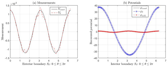
Figure 11. (a) Exact measurement V (black line) and with error $V_{\delta }$ (red line). (b) Exact potential $\phi$ and its approximations ${\phi }_{\alpha \left(\delta \right)}$ and ${\phi }_{\delta }$, corresponding to Example 1 for $\beta =6.3$, $m=12$, and $\delta =0.1$ (see Table 9). In this case, we take $\alpha \left(\delta \right)={10}^{-8}$ and $N=20$.

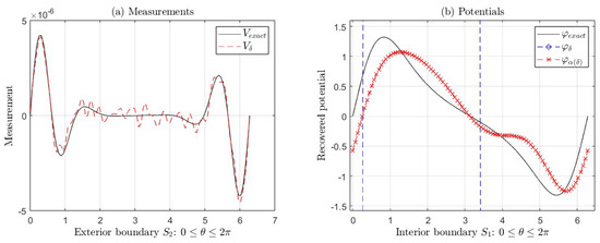
Figure 12. (a) Exact measurement V (black line) and with error $V_{\delta }$ (red line). (b) Exact potential $\phi$ and its approximations ${\phi }_{\alpha \left(\delta \right)}$ and ${\phi }_{\delta }$, corresponding to Example 2 for $\beta =0.5$, $m=8$, and $\delta =0.1$ (see Table 10). In this case, we take $\alpha \left(\delta \right)=5\times {10}^{-17}$ and $N=30$.

4.2.5. Case 5: $\beta <m-1$, When $\beta$ Is Next to n or $n-1$, Where $0<n\le m-1$, for $m=2,\dots ,12$ and $\delta =0.1$

In this section, we consider the case when $\beta <m-1$, when $\beta$ is next to n or $n-1$, where $0<n\le m-1$, for $m=2,\dots ,12$ and $\delta =0.1$. Table 11 and Table 12 show the relative errors of the approximations ${\phi }_{\alpha \left(\delta \right)}$ and ${\phi }_{\delta }$ when $\delta =0.1$ for the same two exact functions $\phi$ considered in Section 4.1.

Table 11. Case 5: Numerical results applying TRM to solve the IP related to the fractional Cauchy problem (12) for $\delta =0.1$ and different values of $\beta$ and m, where $\phi (x,y)=x^2-y^2$, $(x,y)\in S_1$.

N	$\mathit{\alpha }\left(\mathit{\delta }\right)$	$\mathit{\beta }$	m	$\mathit{RE}(\mathit{V},{\mathit{V}}_{\mathit{\delta }})$	$\mathit{RE}(\mathit{\phi },{\mathit{\phi }}_{\mathit{\alpha }\left(\mathit{\delta }\right)})$	$\mathit{RE}(\mathit{\phi },{\mathit{\phi }}_{\mathit{\delta }})$
20	1 × ${10}^{-4}$	0.1	2	0.0981	0.0294	0.0312
20	1 × ${10}^{-4}$	0.0001	2	0.0880	0.0665	0.0702
20	1 × ${10}^{-4}$	0.0000001	2	0.0877	0.0420	0.0436
20	1 × ${10}^{-2}$	0.9	2	0.0825	0.0252	0.0301
20	1 × ${10}^{-2}$	0.9999	2	0.0896	0.0355	0.0383
20	1 × ${10}^{-2}$	0.9999999	2	0.0988	0.0497	0.0524
20	1 × ${10}^{-7}$	0.1	3	0.0984	0.0736	0.4041
20	1 × ${10}^{-7}$	0.0001	3	0.0988	0.0556	0.2586
20	1 × ${10}^{-7}$	0.0000001	3	0.1063	0.0633	0.5828
20	1 × ${10}^{-5}$	0.9	3	0.0824	0.0632	0.2671
20	1 × ${10}^{-4}$	0.9999	3	0.0940	0.0747	0.4997
20	5 × ${10}^{-5}$	0.9999999	3	0.0843	0.0582	0.2323
20	1 × ${10}^{-2}$	2.1	4	0.1133	0.0813	0.4297
20	1 × ${10}^0$	2.9	4	0.1097	0.0494	0.2746
20	1 × ${10}^{-4}$	3.1	5	0.0841	0.0521	0.5721
20	1 × ${10}^{-1}$	3.9	5	0.0923	0.0284	0.9725
20	1 × ${10}^{-1}$	4.1	6	0.0982	0.0441	1.3912
20	1 × ${10}^1$	4.9	6	0.1192	0.0261	0.2905
20	1 × ${10}^{-2}$	5.1	7	0.1027	0.0331	12.2005
20	1 × ${10}^0$	5.9	7	0.0926	0.0324	2.2300
20	1 × ${10}^{-3}$	5.1	8	0.0928	0.0306	2.3248
20	1 × ${10}^{-3}$	5.0001	8	0.0936	0.0312	5.2064
20	1 × ${10}^{-18}$	5.0000001	8	0.1020	0.0174	1.3253
20	1 × ${10}^0$	5.9	8	0.0967	0.0113	3.4116
20	1 × ${10}^0$	5.9999	8	0.0946	0.0260	7.0605
20	1 × ${10}^{-15}$	5.9999999	8	0.0907	0.0275	1.9174
20	1 × ${10}^{-1}$	7.1	9	0.0849	0.0118	9.9754
20	1 × ${10}^0$	7.9	9	0.0916	0.0224	16.5564
20	1 × ${10}^{-13}$	3.1	10	0.0930	0.0114	20.7949
20	1 × ${10}^{-11}$	3.9	10	0.1054	0.0197	31.4437
20	1 × ${10}^{-10}$	6.1	11	0.0978	0.0207	79.4649
20	1 × ${10}^{-7}$	6.9	11	0.1048	0.0109	59.7459
20	1 × ${10}^{-15}$	4.1	12	0.1035	0.0133	108.9786
20	1 × ${10}^{-12}$	4.9	12	0.0978	0.0278	131.9629

Table 12. Case 5: Numerical results applying TRM to solve the IP related to the fractional Cauchy problem (12) for $\delta =0.1$ and different values of $\beta$ and m, where $\phi (x,y)=e^{x}sin\left(y\right)$, $(x,y)\in S_1$.

N	$\mathit{\alpha }\left(\mathit{\delta }\right)$	$\mathit{\beta }$	m	$\mathit{RE}(\mathit{V},{\mathit{V}}_{\mathit{\delta }})$	$\mathit{RE}(\mathit{\phi },{\mathit{\phi }}_{\mathit{\alpha }\left(\mathit{\delta }\right)})$	$\mathit{RE}(\mathit{\phi },{\mathit{\phi }}_{\mathit{\delta }})$
30	1 × ${10}^{-5}$	0.1	2	0.1918	0.0633	0.0669
30	1 × ${10}^{-5}$	0.0001	2	0.1747	0.0510	0.0551
30	1 × ${10}^{-5}$	0.0000001	2	0.1932	0.0408	0.0466
30	1 × ${10}^{-3}$	0.9	2	0.1678	0.0267	0.0338
30	1 × ${10}^{-2}$	0.9999	2	0.1879	0.0538	0.0996
30	1 × ${10}^{-3}$	0.9999999	2	0.1757	0.0330	0.0352
30	7 × ${10}^{-9}$	0.1	3	0.2035	0.1269	0.3288
30	3 × ${10}^{-9}$	0.0001	3	0.1945	0.0741	0.2384
30	6 × ${10}^{-10}$	0.0000001	3	0.1863	0.2035	0.2102
30	7 × ${10}^{-7}$	0.9	3	0.2208	0.1301	0.2493
30	2 × ${10}^{-6}$	0.9999	3	0.2057	0.0770	0.2885
30	5 × ${10}^{-7}$	0.9999999	3	0.2013	0.1809	0.2036
30	1 × ${10}^{-5}$	2.1	4	0.2001	0.1393	0.1397
30	3 × ${10}^{-2}$	2.9	4	0.1984	0.1061	0.2367
30	2 × ${10}^{-4}$	3.1	5	0.2106	0.2788	14.4371
30	6 × ${10}^{-3}$	3.9	5	0.1827	0.2914	6.9833
30	1 × ${10}^{-2}$	4.1	6	0.2299	0.3008	4.2311
30	5 × ${10}^{-1}$	4.9	6	0.1770	0.2723	3.9078
30	3 × ${10}^{-3}$	5.1	7	0.2095	0.1755	297.5818
30	5 × ${10}^{-2}$	5.9	7	0.1969	0.3580	51.0331
30	2 × ${10}^{-3}$	5.1	8	0.2424	0.2924	216.7317
30	3 × ${10}^{-3}$	5.0001	8	0.2004	0.3714	452.3457
30	1.4 × ${10}^{-3}$	5.0000001	8	0.1747	0.3650	239.9826
30	2 × ${10}^2$	5.9	8	0.2001	0.3549	263.7365
30	1.3 × ${10}^{-1}$	5.9999	8	0.1829	0.3781	78.5332
30	5 × ${10}^{-1}$	5.9999999	8	0.2137	0.2490	311.6103
30	1.5 × ${10}^2$	7.1	9	0.2263	0.8972	4.5033 × ${10}^3$
30	1 × ${10}^4$	7.9	9	0.2228	0.8943	4.3085 × ${10}^3$
30	1 × ${10}^{-10}$	3.1	10	0.2658	0.8914	7.9703 × ${10}^3$
30	8 × ${10}^{-8}$	3.9	10	0.2642	0.8948	5.5828 × ${10}^3$
30	1 × ${10}^{-4}$	6.1	11	0.2378	0.9312	2.8572 × ${10}^5$
30	5 × ${10}^{-3}$	6.9	11	0.2089	0.8950	5.1113 × ${10}^4$
30	2 × ${10}^{-11}$	4.1	12	0.2311	0.8945	7.0888 × ${10}^4$
30	4 × ${10}^{-9}$	4.9	12	0.1994	0.9057	7.9818 × ${10}^4$

In Table 11, we observe that $RE(\phi ,{\phi }_{\alpha \left(\delta \right)})<RE(V,V_{\delta })$. For $m=2$, we can see that $RE(\phi ,{\phi }_{\alpha \left(\delta \right)})$ and $RE(\phi ,{\phi }_{\delta })$ are of the same order when $\beta$ is next to 1 or 0 (taking $n=1$), i.e., the solutions without regularization ${\phi }_{\delta }$ are close to regularized solutions ${\phi }_{\alpha \left(\delta \right)}$. However, the regularized approximates ${\phi }_{\alpha \left(\delta \right)}$ are better than the solutions without regularization. The $RE(\phi ,{\phi }_{\alpha \left(\delta \right)})$ increases faster than the $RE(V,V_{\delta })$ starting at $m=3$, as shown in Figure 13b for $\beta =0.0001$, $m=3$, and $\delta =0.1$, where $RE(\phi ,{\phi }_{\alpha \left(\delta \right)})=0.0556$ and $RE(\phi ,{\phi }_{\delta })=0.2586$. These approximations, ${\phi }_{\alpha \left(\delta \right)}$ and ${\phi }_{\delta }$, are recovered from measurements with error $V_{\delta }$, shown in Figure 13a. Also, we can observe similar results in Table 12, where $RE(\phi ,{\phi }_{\alpha \left(\delta \right)})$ and $RE(\phi ,{\phi }_{\delta })$ are of the same order for $m=2$, 3, 4, and when $\beta$ is next to n or $n-1$ (taking $n=1$, 1, and 3, respectively), for $\delta =0.1$, nevertheless the $RE(\phi ,{\phi }_{\alpha \left(\delta \right)})$ increases between 17% and 38%, but no more than the $RE(\phi ,{\phi }_{\delta })$ for $m=5$, 6, 7, and 8. For the values of $m=9$, 10, 11, and 12, the $RE(\phi ,{\phi }_{\alpha \left(\delta \right)})$ increases around 90%, but no more than $RE(\phi ,{\phi }_{\delta })$. In this case, we could use the regularized solution ${\phi }_{\alpha \left(\delta \right)}$ as an initial point of an iterative method to recover a better solution to the IP. Nevertheless, the relative errors of the recovered solutions ${\phi }_{\delta }$ without applying regularization increase suddenly, starting at $m=7$ and $m=5$ (see Table 11 and Table 12) for the functions $\phi (x,y)=x^2-y^2$ and $\phi (x,y)=e^{x}sin\left(y\right)$ for $(x,y)\in S_1$, respectively. Here, the regularization parameters $\alpha \left(\delta \right)$ also change depending on $V_{\delta }$, N, m, and $\beta$.

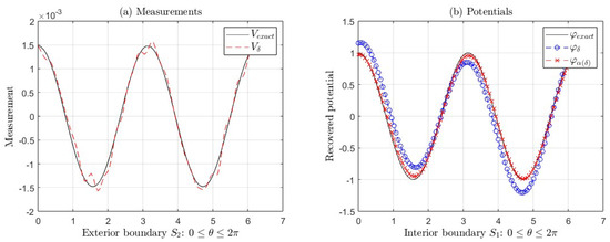
Figure 13. (a) Exact measurement V (black line) and with error $V_{\delta }$ (red line). (b) Exact potential $\phi$ and its approximations ${\phi }_{\alpha \left(\delta \right)}$ and ${\phi }_{\delta }$, corresponding to Example 1 for $\beta =0.0001$, $m=3$, and $\delta =0.1$ (see Table 11). In this case, we take $\alpha \left(\delta \right)={10}^{-7}$ and $N=20$.

Figure 13, Figure 14, Figure 15 and Figure 16 show the graphs of the exact measurement V and with error $V_{\delta }$ with $\delta =0.1$, the graphs of the exact potential $\phi$ and its approximations ${\phi }_{\alpha \left(\delta \right)}$ (with regularization) and ${\phi }_{\delta }$ (without regularization), corresponding to the functions $\phi (x,y)=x^2-y^2$ and $\phi (x,y)=e^{x}sin\left(y\right)$ for $(x,y)\in S_1$, respectively. In both cases, as mentioned in the previous paragraph, the errors increase suddenly, starting at $m=7$ for the first function and starting at $m=5$ for the second one, as can be seen in Figure 14b, Figure 15b, and Figure 16b, where we can see the ill-posedness of the IP if we do not apply regularization for $m=12$, 8, and $m=11$, respectively. For example, for the approximations ${\phi }_{\delta }$ and ${\phi }_{\alpha \left(\delta \right)}$ shown in Figure 14b of the first function, the $RE(\phi ,{\phi }_{\delta })=131.9629$ is much greater than $RE(\phi ,{\phi }_{\alpha \left(\delta \right)})=0.0278$ for $\beta =4.9$, $m=12$, and $\delta =0.1$ (see Table 11). For the approximations ${\phi }_{\delta }$ and ${\phi }_{\alpha \left(\delta \right)}$ shown in Figure 15b of the second one, the $RE(\phi ,{\phi }_{\delta })=78.5332$ is much greater than $RE(\phi ,{\phi }_{\alpha \left(\delta \right)})=0.3781$, for $\beta =5.9999$, $m=8$, and y $\delta =0.1$ (see Table 12). Lastly, for the approximations ${\phi }_{\delta }$ and ${\phi }_{\alpha \left(\delta \right)}$ shown in Figure 16b of the second one, the $RE(\phi ,{\phi }_{\delta })=2.8572\times {10}^5$ is greater than $RE(\phi ,{\phi }_{\alpha \left(\delta \right)})=0.9312$ for $\beta =6.1$, $m=11$, and $\delta =0.1$ (see Table 12). In these last two examples, when the approximate solutions ${\phi }_{\alpha \left(\delta \right)}$ are not close to the exact solution $\phi$, we could use the regularized solution ${\phi }_{\alpha \left(\delta \right)}$ as an initial point of an iterative method to recover a better solution to the IP.

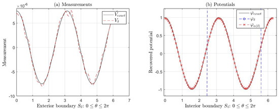
Figure 14. (a) Exact measurement V (black line) and with error $V_{\delta }$ (red line). (b) Exact potential $\phi$ and its approximations ${\phi }_{\alpha \left(\delta \right)}$ and ${\phi }_{\delta }$, corresponding to Example 1 for $\beta =4.9$, $m=12$, and $\delta =0.1$ (see Table 11). In this case, we take $\alpha \left(\delta \right)={10}^{-12}$ and $N=20$.

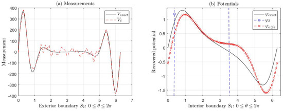
Figure 15. (a) Exact measurement V (black line) and with error $V_{\delta }$ (red line). (b) Exact potential $\phi$ and its approximations ${\phi }_{\alpha \left(\delta \right)}$ and ${\phi }_{\delta }$, corresponding to Example 2 for $\beta =5.9999$, $m=8$, and $\delta =0.1$ (see Table 12). In this case, we take $\alpha \left(\delta \right)=1.3\times {10}^{-1}$ and $N=30$.

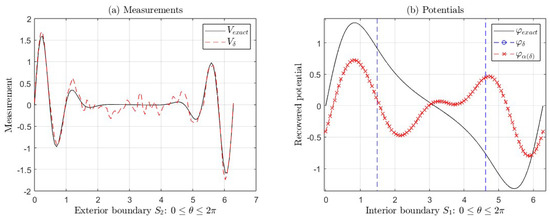
Figure 16. (a) Exact measurement V (black line) and with error $V_{\delta }$ (red line). (b) Exact potential $\phi$ and its approximations ${\phi }_{\alpha \left(\delta \right)}$ and ${\phi }_{\delta }$, corresponding to Example 2 for $\beta =6.1$, $m=11$, and $\delta =0.1$ (see Table 12). In this case, we take $\alpha \left(\delta \right)={10}^{-4}$ and $N=30$.

4.2.6. Case 6: $\beta >m$, for $m=1,2$,…,13 and $\delta =0.1$

In this case, we consider the case when $\beta >m$, with $m=1,2,\dots ,13.$ for $\delta =0.1$. Table 13 and Table 14 show the relative errors of the approximations ${\phi }_{\alpha \left(\delta \right)}$ and ${\phi }_{\delta }$ when $\delta =0.1$ for the same two exact functions $\phi$ considered in Section 4.1.

Table 13. Case 6: Numerical results applying TRM to solve IP related to the fractional Cauchy problem (12) for $\delta =0.1$ and different values of $\beta$ and m, where $\phi (x,y)=x^2-y^2$, $(x,y)\in S_1$.

N	$\mathit{\alpha }\left(\mathit{\delta }\right)$	$\mathit{\beta }$	m	$\mathit{RE}(\mathit{V},{\mathit{V}}_{\mathit{\delta }})$	$\mathit{RE}(\mathit{\phi },{\mathit{\phi }}_{\mathit{\alpha }\left(\mathit{\delta }\right)})$	$\mathit{RE}(\mathit{\phi },{\mathit{\phi }}_{\mathit{\delta }})$
20	1 × ${10}^{-6}$	1.001	1	0.0949	0.0430	0.0432
20	1 × ${10}^{14}$	1.5	1	0.0860	0.0825	0.0965
20	1 × ${10}^{-6}$	2.0001	2	0.0911	0.0574	0.0581
20	1 × ${10}^{32}$	3.1	2	0.0809	0.0783	0.0863
20	1 × ${10}^{-1}$	3.01	3	0.0894	0.0278	0.1076
20	1 × ${10}^{45}$	4.5	3	0.1048	0.0639	0.2370
20	1 × ${10}^5$	4.1	4	0.0942	0.0294	0.1592
20	1 × ${10}^{95}$	7.1	4	0.1051	0.0495	0.2588
20	1 × ${10}^{-4}$	5.0001	5	0.0792	0.0298	1.3533
20	1 × ${10}^{33}$	6.1	5	0.0946	0.0165	0.4475
20	1 × ${10}^6$	6.1	6	0.0907	0.0277	0.9987
20	1 × ${10}^{48}$	7.5	6	0.0867	0.0276	0.6014
20	1 × ${10}^5$	7.1	7	0.0932	0.0109	3.5379
20	1 × ${10}^{50}$	8.6	7	0.1024	0.0131	3.1745
20	1 × ${10}^1$	8.001	8	0.1135	0.0277	2.2757
20	1 × ${10}^{46}$	9.4	8	0.0877	0.0180	3.6123
20	1 × ${10}^{-2}$	9.0001	9	0.0935	0.0163	22.9725
20	1 × ${10}^{53}$	10.7	9	0.0979	0.0342	3.1946
20	1 × ${10}^{-1}$	10.0001	10	0.1046	0.0345	50.3389
20	1 × ${10}^{49}$	11.5	10	0.0979	0.0179	12.7233
20	1 × ${10}^0$	11.001	11	0.0834	0.0164	12.8627
20	1 × ${10}^{53}$	12.6	11	0.0915	0.0331	44.9837
20	1 × ${10}^1$	12.0001	12	0.1136	0.0195	121.2423
20	1 × ${10}^{47}$	13.4	12	0.0822	0.0165	113.4837
20	1 × ${10}^1$	11.5	13	0.0941	0.0155	420.7545
20	1 × ${10}^3$	12.0001	13	0.0950	0.0280	319.2454
20	1 × ${10}^4$	12.5	13	0.1188	0.0187	701.4226
20	1 × ${10}^1$	12.9999	13	0.0925	0.0198	183.4905
20	1 × ${10}^{29}$	13.5	13	0.0938	0.0219	400.2461
20	1 × ${10}^{51}$	14.5	13	0.1112	0.0295	319.4336

Table 14. Case 6: Numerical results applying TRM to solve IP related to the fractional Cauchy problem (12) for $\delta =0.1$ and different values of $\beta$ and m, where $\phi (x,y)=e^{x}sin\left(y\right)$, $(x,y)\in S_1$.

N	$\mathit{\alpha }\left(\mathit{\delta }\right)$	$\mathit{\beta }$	m	$\mathit{RE}(\mathit{V},{\mathit{V}}_{\mathit{\delta }})$	$\mathit{RE}(\mathit{\phi },{\mathit{\phi }}_{\mathit{\alpha }\left(\mathit{\delta }\right)})$	$\mathit{RE}(\mathit{\phi },{\mathit{\phi }}_{\mathit{\delta }})$
30	3 × ${10}^{-5}$	1.001	1	0.1942	0.0575	0.1229
30	3 × ${10}^{13}$	1.5	1	0.1687	0.0687	0.0965
30	6 × ${10}^{-6}$	2.0001	2	0.1681	0.0606	0.1017
30	1 × ${10}^{32}$	3.1	2	0.1800	0.0660	0.0763
30	2 × ${10}^{-2}$	3.01	3	0.1855	0.1200	0.5139
30	5 × ${10}^{44}$	4.5	3	0.2034	0.1517	1.0728
30	3 × ${10}^3$	4.1	4	0.1930	0.0226	0.3616
30	5 × ${10}^{93}$	7.1	4	0.2236	0.1517	0.4427
30	3.1 × ${10}^{-5}$	5.0001	5	0.2254	0.1550	13.8261
30	1.1 × ${10}^{32}$	6.1	5	0.2046	0.1057	3.5558
30	6.3 × ${10}^{-4}$	6.0001	6	0.1984	0.1863	8.7178
30	6.4 × ${10}^{46}$	7.5	6	0.2036	0.1233	4.9854
30	6.5 × ${10}^4$	7.1	7	0.2188	0.3310	253.4635
30	4.4 × ${10}^{36}$	8.2	7	0.1844	0.2976	36.0590
30	3.4 × ${10}^{-4}$	8.00001	8	0.1944	0.4695	460.0541
30	1.1 × ${10}^{57}$	9.8	8	0.2512	0.4601	157.1510
30	3 × ${10}^1$	9.0001	9	0.2299	0.8871	7.2299 × ${10}^3$
30	5.1 × ${10}^{57}$	10.7	9	0.2143	0.8912	4.4110 × ${10}^3$
30	5 × ${10}^2$	10.0001	10	0.2151	0.8907	2.0204 × ${10}^4$
30	1 × ${10}^{53}$	11.5	10	0.2191	0.8920	2.4527 × ${10}^3$
30	6 × ${10}^3$	11.0001	11	0.2632	0.8857	3.6429 × ${10}^5$
30	9 × ${10}^{50}$	12.4	11	0.2290	0.9571	1.8509 × ${10}^5$
30	1.3 × ${10}^5$	12.0001	12	0.2451	0.9564	3.7314 × ${10}^5$
30	2.1 × ${10}^{52}$	13.4	12	0.2211	0.9192	4.5936 × ${10}^5$
30	5.9 × ${10}^{10}$	11.5	13	0.2168	0.9964	1.3190 × ${10}^7$
30	5 × ${10}^{11}$	12.0001	13	0.2607	0.9994	1.0836 × ${10}^5$
30	9 × ${10}^{11}$	12.5	13	0.2326	0.9904	1.0214 × ${10}^7$
30	1.1 × ${10}^9$	12.9999	13	0.2439	0.9890	1.3107 × ${10}^7$
30	1.3 × ${10}^{29}$	13.5	13	0.2338	0.9895	5.7405 × ${10}^6$
30	1.7 × ${10}^{59}$	14.5	13	0.2424	0.9899	1.3997 × ${10}^7$

In Table 13, we observe that $RE(\phi ,{\phi }_{\alpha \left(\delta \right)})<RE(V,V_{\delta })$. For $m=1,2$, we can see that $RE(\phi ,{\phi }_{\alpha \left(\delta \right)})$ and $RE(\phi ,{\phi }_{\delta })$ are of the same order when $\delta =0.1$, i.e., the solutions without regularization ${\phi }_{\delta }$ are close to regularized solutions ${\phi }_{\alpha \left(\delta \right)}$. However, the regularized approximates ${\phi }_{\alpha \left(\delta \right)}$ are better than the solutions without regularization. Additionally, the relative errors of the solutions without regularization ${\phi }_{\delta }$ increase faster, starting at $m=3$. Furthermore, we can observe similar results in Table 14. In this case, the relative errors from solutions with regularization $RE(\phi ,{\phi }_{\alpha \left(\delta \right)})$ are less than the $RE(V,V_{\delta })$ for $m=1,2,\dots ,6$, and increase between 29% and 46% for $m=7,8$, when $\delta =0.1$. Nevertheless, the corresponding relative errors of the solutions with regularization increase between 88% and 96% for $m=9,10,11,12$, but no more than the corresponding $RE(\phi ,{\phi }_{\delta })$. The relative errors of the recovered solutions ${\phi }_{\delta }$ without regularization increase suddenly, starting at $m\ge 5$. For example, for $\beta =10.7$ and $m=9$, the $RE(\phi ,{\phi }_{\delta })=4.4110\times {10}^3$. For $m=13$, the $RE(\phi ,{\phi }_{\alpha \left(\delta \right)})$ increases between 91% and 99%, but no more than the $RE(\phi ,{\phi }_{\delta })$), for $\beta >m$, as well as for $\beta <m$ and $m-1<\beta <m$ with $\delta =0.1$. Moreover, as in the previous cases, the regularization parameters $\alpha \left(\delta \right)$ change depending on the data with error $V_{\delta }$, the values N, m, and $\beta$. Analogous results can be obtained for values $m\ge 14$, as those obtained for $m=13$, which are not included in this work.

In the following two examples, we have considered non-smooth functions.

Example 3. 

We consider the ‘exact potential’ $\phi (x,y)=\sqrt{(x^2+y^2)}-\pi /2$, for $(x,y)\in S_1$, which in polar coordinates is given by $\phi \left(\theta \right)=\left|\theta \right|-\pi /2$, for $\theta \in [-\pi ,\pi ]$. Resembling the first example, the ‘exact measurement’ V and the ‘measurement with error’ $V_{\delta }$ are generated with the first N terms of the Fourier series (22) and (23), respectively, such that $\parallel {\phi }_N{-\phi \parallel }_{L_2\left(S_1\right)}\le {ϵ}_F$, with $0\le {ϵ}_F$. For $N=30$, ${ϵ}_F=0.0056$. In this case, $V_0={\phi }_0=0$ and the Fourier coefficients ${\phi }_k,1\le k\le N$, are obtained numerically using the intrinsic function $quadl$ of $MATLAB$.

Table 15 shows the numerical results for data without error, applying TRM to solve the IP of the classical Cauchy problem (2), where $N=20$, 25, and 30. In this table, we can observe similar results to the previous examples where the regularized solutions ${\phi }_{\alpha \left(\delta \right)}$ are better.

Table 15. Numerical results applying TRM to solve the IP related to the classical Cauchy problem (2), for $\phi \left(\theta \right)=\left|\theta \right|-\pi /2$, $\theta \in [-\pi ,\pi ]$ and different values of $\delta$ and N.

$\mathit{\delta }$	N	$\mathit{\alpha }\left(\mathit{\delta }\right)$	$\mathit{RE}(\mathit{V},{\mathit{V}}_{\mathit{\delta }})$	$\mathit{RE}(\mathit{\phi },{\mathit{\phi }}_{\mathit{\alpha }\left(\mathit{\delta }\right)})$	$\mathit{RE}(\mathit{\phi },{\mathit{\phi }}_{\mathit{\delta }})$
0.1	20	0.1	0.1080	0.1545	1.1839
0.1	25	0.1	0.0953	0.1314	2.1403
0.1	30	0.1	0.1342	0.1630	5.5998
0.01	20	0.01	0.0121	0.0409	0.1102
0.01	25	0.01	0.0114	0.0425	0.1676
0.01	30	0.01	0.0128	0.0370	0.5224
0.001	20	0.001	8.1891 × ${10}^{-4}$	0.0043	0.0046
0.001	25	0.001	9.1866 × ${10}^{-4}$	0.0088	0.0139
0.001	30	0.001	0.0014	0.0117	0.0557

Table 16 shows the numerical results for data without error, applying TRM to solve the IP of the fractional Cauchy problem (12) for different values of $\beta$, m, and N.

Table 16. Numerical results applying TRM to solve IP related to the fractional Cauchy problem (12) for $\delta =0.1$ and different values of $\beta$ and m, where $\phi \left(\theta \right)=\left|\theta \right|-\pi /2$, $\theta \in [-\pi ,\pi ]$.

N	$\mathit{\alpha }\left(\mathit{\delta }\right)$	$\mathit{\beta }$	m	$\mathit{RE}(\mathit{V},{\mathit{V}}_{\mathit{\delta }})$	$\mathit{RE}(\mathit{\phi },{\mathit{\phi }}_{\mathit{\alpha }\left(\mathit{\delta }\right)})$	$\mathit{RE}(\mathit{\phi },{\mathit{\phi }}_{\mathit{\delta }})$
20	2 × ${10}^{-3}$	0.5	1	0.3124	0.1870	0.2188
20	2 × ${10}^{-5}$	0.1	1	0.1347	0.1118	0.1121
20	1 × ${10}^{-2}$	0.9	1	0.1180	0.1919	0.2229
20	2 × ${10}^{-4}$	0.1	2	0.1524	0.0594	0.0974
20	1 × ${10}^{-3}$	1.1	2	0.1362	0.1985	0.1989
20	1 × ${10}^{-3}$	1.5	2	0.1047	0.2133	0.2141
20	4.7 × ${10}^0$	1.9	2	0.2123	0.3425	1.3020
10	4.9 × ${10}^{-3}$	2.1	3	0.0523	0.2633	1.9458
10	5 × ${10}^{-3}$	2.5	3	0.0527	0.1430	0.3773
10	2.8 × ${10}^{-1}$	2.9	3	0.0495	0.2678	2.7599
10	2.1 × ${10}^0$	3.5	4	0.0463	0.2386	1.8027
8	1 × ${10}^{-1}$	4.1	5	0.0397	0.4832	48.7338
8	4.2 × ${10}^{-1}$	4.5	5	0.0378	0.3875	24.7968
8	2.8 × ${10}^0$	4.9	5	0.0269	0.4535	27.6306
8	1 × ${10}^2$	5.9	6	0.0281	0.2041	23.2792
6	1 × ${10}^1$	6.9	7	0.0207	0.2113	105.7357
6	7.2 × ${10}^1$	7.1	8	0.0257	0.5941	280.7669
4	2.2 × ${10}^1$	9.1	10	0.0416	0.2823	79.7393
4	3.3 × ${10}^0$	10.1	11	0.0265	0.1181	1.4592 × ${10}^3$
4	2.5 × ${10}^2$	11.1	12	0.0306	0.1032	1.0285 × ${10}^3$
4	2.2 × ${10}^2$	12.5	13	0.0348	0.7974	1.0332 × ${10}^4$

Figure 17a,b show the graphs of the exact potential $\phi$ and its approximations ${\phi }_{\alpha \left(\delta \right)}$ (with regularization) and ${\phi }_{\delta }$ (without regularization), corresponding to the function $\phi \left(\theta \right)=\left|\theta \right|-\pi /2$, for $\theta \in [-\pi ,\pi ]$, for different values of $\beta$, m, and N, respectively.

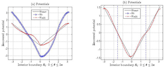
Figure 17. (a) Exact potential $\phi$ and its approximations ${\phi }_{\alpha \left(\delta \right)}$ and ${\phi }_{\delta }$, corresponding to Example 3 for $\beta =1.9$, $m=2$, $N=20$, and $\delta =0.1$. (b) Exact potential $\phi$ and its approximations ${\phi }_{\alpha \left(\delta \right)}$ and ${\phi }_{\delta }$, corresponding to Example 3 for $\beta =11.1$, $m=12$, $N=4$, and $\delta =0.1$ (see Table 16).

Example 4. 

We consider the ‘exact potential’ in polar coordinates given by $\phi \left(\theta \right)=-1$ if $\theta \in [-\pi ,0)$ and 1 if $\theta \in [0,\pi ]$. Similar to the first example, the ‘exact measurement’ V and the ‘measurement with error’ $V_{\delta }$ are generated with the first N terms of the Fourier series (22) and (23), respectively, such that $\parallel {\phi }_N{-\phi \parallel }_{L_2\left(S_1\right)}\le {ϵ}_F$, with $0\le {ϵ}_F$. For $N=30$, ${ϵ}_F=0.2913$. In this case, $V_0={\phi }_0=0$, and the Fourier coefficients ${\phi }_k,1\le k\le N$, are obtained numerically using the intrinsic function $quadl$ of $MATLAB$.

Table 17 shows the numerical results for data without error, applying TRM to solve the IP of the classical Cauchy problem (2), where $N=20$, 25, and 30. In this table, we can observe similar results to the previous examples where the regularized solutions ${\phi }_{\alpha \left(\delta \right)}$ are better.

Table 17. Numerical results applying TRM to solve the IP related to the classical Cauchy problem (2), for $\phi \left(\theta \right)=-1$ if $\theta \in [-\pi ,0)$ and 1 if $\theta \in [0,\pi ]$, and different values of $\delta$ and N.

$\mathit{\delta }$	N	$\mathit{\alpha }\left(\mathit{\delta }\right)$	$\mathit{RE}(\mathit{V},{\mathit{V}}_{\mathit{\delta }})$	$\mathit{RE}(\mathit{\phi },{\mathit{\phi }}_{\mathit{\alpha }\left(\mathit{\delta }\right)})$	$\mathit{RE}(\mathit{\phi },{\mathit{\phi }}_{\mathit{\delta }})$
0.1	20	0.1	0.0666	0.1608	0.7217
0.1	25	0.1	0.0638	0.1702	0.7641
0.1	30	0.1	0.0767	0.1827	2.6840
0.01	20	0.01	0.0080	0.0544	0.0659
0.01	25	0.01	0.0068	0.0761	0.0998
0.01	30	0.01	0.0078	0.0946	0.3552
0.001	20	0.0001	7.6172 × ${10}^{-4}$	0.0044	0.0048
0.001	25	0.0001	7.2529 × ${10}^{-4}$	0.0099	0.0118
0.001	30	0.0001	9.2391 × ${10}^{-4}$	0.0195	0.0353

Table 18 shows the numerical results for data without error, applying TRM to solve the IP of the fractional Cauchy problem (12) for different values of $\beta$, m, and N.

Table 18. Numerical results applying TRM to solve IP related to the fractional Cauchy problem (12) for $\delta =0.1$ and different values of $\beta$ and m, where $\phi \left(\theta \right)=-1$ if $\theta \in [-\pi ,0)$ and 1 if $\theta \in [0,\pi ]$.

N	$\mathit{\alpha }\left(\mathit{\delta }\right)$	$\mathit{\beta }$	m	$\mathit{RE}(\mathit{V},{\mathit{V}}_{\mathit{\delta }})$	$\mathit{RE}(\mathit{\phi },{\mathit{\phi }}_{\mathit{\alpha }\left(\mathit{\delta }\right)})$	$\mathit{RE}(\mathit{\phi },{\mathit{\phi }}_{\mathit{\delta }})$
20	4.5 × ${10}^{-2}$	0.5	1	0.1062	0.2731	1.9413
10	3.9 × ${10}^{-4}$	0.1	1	0.0645	0.0729	0.1759
10	3.2 × ${10}^{-3}$	0.5	1	0.0640	0.1624	0.2390
10	4 × ${10}^{-3}$	0.9	1	0.0609	0.0841	0.0934
10	2.1 × ${10}^{-2}$	1.2	2	0.0910	0.1530	0.1636
10	1.5 × ${10}^{-3}$	1.5	2	0.0549	0.2629	0.2699
6	2.1 × ${10}^{-2}$	2.5	3	0.0352	0.3415	1.3513
6	1.5 × ${10}^0$	3.5	4	0.0523	0.5428	1.1704
6	1 × ${10}^3$	4.2	5	0.0472	0.9410	88.1158
6	3.6 × ${10}^4$	5.2	6	0.0483	0.9354	41.0394
6	1.5 × ${10}^7$	7.2	8	0.0400	0.9343	1.7546 × ${10}^3$
6	4.2 × ${10}^{16}$	12.8	13	0.0606	0.9825	2.1740 × ${10}^7$

Figure 18a,b show the graphs of the exact potential $\phi$ and its approximations ${\phi }_{\alpha \left(\delta \right)}$ (with regularization) and ${\phi }_{\delta }$ (without regularization), corresponding to the function $\phi \left(\theta \right)=-1$ if $\theta \in [-\pi ,0)$ and 1 if $\theta \in [0,\pi ]$, for $\theta \in [-\pi ,\pi ]$, for different values of $\beta$, m, and N, respectively.

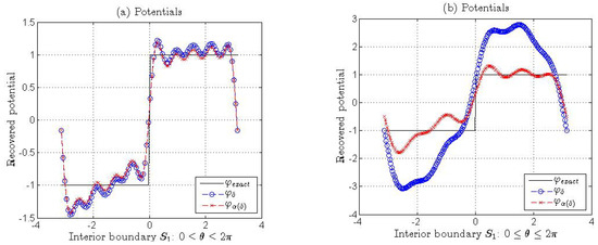
Figure 18. (a) Exact potential $\phi$ and its approximations ${\phi }_{\alpha \left(\delta \right)}$ and ${\phi }_{\delta }$, corresponding to Example 4 for $\beta =1.2$, $m=2$, $N=10$, and $\delta =0.1$. (b) Exact potential $\phi$ and its approximations ${\phi }_{\alpha \left(\delta \right)}$ and ${\phi }_{\delta }$, corresponding to Example 4 for $\beta =2.5$, $m=3$, $N=6$, and $\delta =0.1$ (see Table 18).

Examples 3 and 4 show numerical results analogous to the previous examples for both the classical and fractional cases. However, when we have piecewise constant functions, we truncate the series of approximate solutions ${\phi }_{\alpha \left(\delta \right)}$ to find a better approximation of the solution to the fractional Cauchy problem.

4.3. Solution to the IP Related to the Fractional Cauchy Problem Morozov Discrepancy Method and the Criterion of Tikhonov

In this subsection, the numerical results of the approximate solutions of the four examples presented above are calculated by the proposed method, choosing the regularization parameter by Morozov’s discrepancy method and by the Tikhonov criterion. The relative errors of the approximations given in Table 19, Table 20, Table 21, Table 22, Table 23, Table 24, Table 25 and Table 26 show that the best approximate solutions to the inverse problem are obtained by the L-curve criterion, as shown in Table 13, Table 14, Table 16, and Table 18, taking the same values of N, $\alpha$, $\beta$, and m from these same examples for Table 19, Table 20, Table 21, Table 22, Table 23, Table 24, Table 25 and Table 26, respectively.

Table 19. Numerical results choosing the regularization parameter $\alpha \left(\delta \right)$ with the discrepancy principle of Morozov to solve IP related to the fractional Cauchy problem (12) for $\delta =0.1$ and different values of $\beta$ and m, where $\phi (x,y)=x^2-y^2$, $(x,y)\in S_1$. According to the results of the table and additional experiments, the discrepancy method fails when $\beta >(m+1)$ and $m>1$, as well as for some values of $\beta <(m-1)$.

N	$\mathit{\alpha }\left(\mathit{\delta }\right)$	$\mathit{\beta }$	m	$\mathit{RE}(\mathit{V},{\mathit{V}}_{\mathit{\delta }})$	$\mathit{RE}(\mathit{\phi },{\mathit{\phi }}_{\mathit{\alpha }\left(\mathit{\delta }\right)})$	$\mathit{RE}(\mathit{\phi },{\mathit{\phi }}_{\mathit{\delta }})$
20	0.1613	1.001	1	0.0959	1.0470	0.0972
20	7.5089 × ${10}^6$	1.5	1	0.0983	0.1328	0.1328
20	1.03 × ${10}^3$	2.0001	2	0.0827	1.0000	0.0418
20	NaN	3.1	2	0.0870	NaN	0.0259
20	0.3137	3.01	3	0.0921	0.0526	0.1290
20	NaN	4.5	3	0.0994	NaN	0.4877
20	17.79	4.1	4	0.1069	0.5115	0.5102
20	NaN	7.1	4	0.0949	NaN	0.1675
20	6.53 × ${10}^7$	5.0001	5	0.0901	1.0000	1.2477
20	NaN	6.1	5	0.0965	NaN	1.4885
20	4.7570	6.1	6	0.0860	1.9250	1.9237
20	NaN	7.5	6	0.0932	NaN	1.9387
20	0.2678	7.1	7	0.0922	6.1441	6.1514
20	NaN	8.6	7	0.0983	NaN	8.3501
20	0.0909	8.001	8	0.1113	0.0995	1.4459
20	NaN	9.4	8	0.0947	NaN	3.8687
20	0.1659	9.0001	9	0.0913	0.0497	9.9648
20	NaN	10.7	9	0.1018	NaN	21.7190
20	3.7653 × ${10}^{-5}$	10.0001	10	0.0818	23.2250	36.9474
20	NaN	11.5	10	0.0980	NaN	34.1752
20	3.1198 × ${10}^{-5}$	11.001	11	0.0828	50.0333	57.7211
20	NaN	12.6	11	0.0827	NaN	105.6237
20	1.0869 × ${10}^{-5}$	12.0001	12	0.0892	80.4548	94.1772
20	NaN	13.4	12	0.0852	NaN	13.4034
20	NaN	11.5	13	0.0984	NaN	517.1635
20	5.1280 × ${10}^{-6}$	12.0001	13	0.1027	780.2431	783.2423
20	4.8277 × ${10}^{-5}$	12.5	13	0.1031	292.2405	293.0910
20	1.03160 × ${10}^{-6}$	12.9999	13	0.0971	148.1006	226.6417
20	3.4578 × ${10}^3$	13.5	13	0.1041	597.4911	597.4911
20	NaN	14.5	13	0.0747	NaN	105.6650

Table 20. Numerical results choosing the regularization parameter $\alpha \left(\delta \right)$ with the Tikhonov criterion to solve IP related to the fractional Cauchy problem (12) for $\delta =0.1$ and different values of $\beta$ and m, where $\phi (x,y)=x^2-y^2$, $(x,y)\in S_1$. Similar results have been obtained for other values of $\alpha$ using this criterion.

N	$\mathit{\alpha }\left(\mathit{\delta }\right)$	$\mathit{\beta }$	m	$\mathit{RE}(\mathit{V},{\mathit{V}}_{\mathit{\delta }})$	$\mathit{RE}(\mathit{\phi },{\mathit{\phi }}_{\mathit{\alpha }\left(\mathit{\delta }\right)})$	$\mathit{RE}(\mathit{\phi },{\mathit{\phi }}_{\mathit{\delta }})$
20	${\delta }^{{\displaystyle \frac{3}{2}}}$	1.001	1	0.0994	0.9040	0.0769
20	${\delta }^{{\displaystyle \frac{3}{2}}}$	1.5	1	0.0965	0.0938	0.0938
20	$1+1=2$${\delta }^{{\displaystyle \frac{99}{50}}}$	2.0001	2	0.1046	0.9022	0.0702
20	$\delta$	3.1	2	0.0984	0.1345	0.1345
20	$\delta$	3.01	3	0.0812	0.0852	0.3750
20	${\delta }^{{\displaystyle \frac{1}{3}}}$	4.5	3	0.0862	0.3665	0.3665
20	${\delta }^{{\displaystyle \frac{1}{100}}}$	4.1	4	0.1050	0.3914	0.3914
20	$\delta$	7.1	4	0.0971	0.8561	0.8561
20	${\delta }^{{\displaystyle \frac{99}{50}}}$	5.0001	5	0.0893	0.5591	1.5529
20	${\delta }^{{\displaystyle \frac{99}{50}}}$	6.1	5	0.0934	1.2559	1.2559
20	${\delta }^{{\displaystyle \frac{1}{3}}}$	6.1	6	0.0929	1.5055	1.5056
20	${\delta }^{{\displaystyle \frac{1}{2}}}$	7.5	6	0.0994	2.0076	2.0076
20	${\delta }^{{\displaystyle \frac{99}{50}}}$	7.1	7	0.0949	2.5857	2.5858
20	${\delta }^{{\displaystyle \frac{99}{50}}}$	8.6	7	0.0913	2.4924	2.4924
20	${\delta }^{{\displaystyle \frac{1}{100}}}$	8.001	8	0.0957	0.0431	5.6199
20	${\delta }^{{\displaystyle \frac{1}{100}}}$	9.4	8	0.0971	13.6930	13.6930
20	${\delta }^{{\displaystyle \frac{1}{10000}}}$	9.0001	9	0.0893	0.3169	24.8451
20	${\delta }^{{\displaystyle \frac{1}{10000}}}$	10.7	9	0.1057	8.4227	8.4227
20	$\delta$	10.0001	10	0.1031	0.0334	25.1034
20	$\delta$	11.5	10	0.0990	28.5194	28.5194
20	${\delta }^{{\displaystyle \frac{99}{10000}}}$	11.001	11	0.0834	0.0225	36.1203
20	${\delta }^{{\displaystyle \frac{99}{10000}}}$	12.6	11	0.0988	66.3421	66.3421
20	${\delta }^{{\displaystyle \frac{1}{100}}}$	12.0001	12	0.1022	0.0279	95.8910
20	${\delta }^{{\displaystyle \frac{1}{100}}}$	13.4	12	0.0926	31.8654	31.8654
20	${\delta }^{{\displaystyle \frac{1}{10000}}}$	11.5	13	0.1099	0.0552	457.5273
20	${\delta }^{{\displaystyle \frac{1}{10000}}}$	12.0001	13	0.1133	0.5851	438.2230
20	${\delta }^{{\displaystyle \frac{1}{10000}}}$	12.5	13	0.1097	4.5644	279.6731
20	${\delta }^{{\displaystyle \frac{1}{10000}}}$	12.9999	13	0.0982	0.0249	358.7193
20	${\delta }^{{\displaystyle \frac{1}{10000}}}$	13.5	13	0.0925	183.5626	183.5626
20	${\delta }^{{\displaystyle \frac{1}{10000}}}$	14.5	13	0.1027	789.7150	789.7150

Table 21. Numerical results applying Morozov discrepancy principle to solve IP related to the fractional Cauchy problem (12) for $\delta =0.1$ and different values of $\beta$ and m, where $\phi (x,y)=e^{x}sin\left(y\right)$, $(x,y)\in S_1$. According to the results, the discrepancy principle has problems when $\beta >m+1$ and $m>1$, and for $\beta =1.001$ and $m=1$.

N	$\mathit{\alpha }\left(\mathit{\delta }\right)$	$\mathit{\beta }$	m	$\mathit{RE}(\mathit{V},{\mathit{V}}_{\mathit{\delta }})$	$\mathit{RE}(\mathit{\phi },{\mathit{\phi }}_{\mathit{\alpha }\left(\mathit{\delta }\right)})$	$\mathit{RE}(\mathit{\phi },{\mathit{\phi }}_{\mathit{\delta }})$
30	NaN	1.001	1	0.1245	NaN	0.0962
30	2.0984 × ${10}^6$	1.5	1	0.1910	0.1082	0.1082
30	1.03 × ${10}^3$	2.0001	2	0.0954	1.0000	0.0244
30	NaN	3.1	2	0.1075	NaN	0.0402
30	0.2289	3.01	3	0.1118	0.0657	0.4844
30	NaN	4.5	3	0.1218	NaN	1.4902
30	49.9604	4.1	4	0.1040	0.1739	0.1726
30	NaN	7.1	4	0.1200	NaN	0.3234
30	6.46 × ${10}^7$	5.0001	5	0.1222	1.0000	1.5949
30	NaN	6.1	5	0.1098	NaN	1.8066
30	0.0725	6.0001	6	0.1133	0.1997	1.9133
30	NaN	7.5	6	0.1058	NaN	1.5889
30	0.1979	7.1	7	0.1126	8.3170	8.3243
30	NaN	8.2	7	0.1207	NaN	4.1606
30	0.0471	8.00001	8	0.1245	0.5043	5.9603
30	NaN	9.8	8	0.1132	NaN	6.3306
30	0.1675	9.0001	9	0.1027	0.0679	15.9717
30	NaN	10.7	9	0.0961	NaN	9.3670
30	0.8716	10.0001	10	0.0954	0.0099	5.1670
30	NaN	11.5	10	0.1075	NaN	8.4426
30	2.7508 × ${10}^{-8}$	11.0001	11	0.2068	5.0164 × ${10}^4$	5.0171 × ${10}^4$
30	NaN	12.4	11	0.1218	NaN	125.4177
30	6.7362 × ${10}^{-9}$	12.0001	12	0.2635	1.1476 × ${10}^5$	1.1477 × ${10}^5$
30	NaN	13.4	12	0.1200	NaN	82.7087
30	1.6116 × ${10}^{-10}$	11.5	13	0.2236	5.6345 × ${10}^6$	5.6345 × ${10}^6$
30	9.6113 × ${10}^{-8}$	12.0001	13	0.2251	3.6801 × ${10}^5$	3.6801 × ${10}^5$
30	3.7943 × ${10}^{-9}$	12.5	13	0.2458	3.2872 × ${10}^6$	3.2872 × ${10}^6$
30	1.2925 × ${10}^{-11}$	12.9999	13	0.2276	1.0450 × ${10}^7$	1.0450 × ${10}^7$
30	NaN	13.5	13	0.2413	NaN	8.8855 × ${10}^6$
30	NaN	14.5	13	0.2454	NaN	9.6411 × ${10}^6$

Table 22. Numerical results choosing the regularization parameter $\alpha \left(\delta \right)$ with the Tikhonov criterion to solve IP related to the fractional Cauchy problem (12) for $\delta =0.1$ and different values of $\beta$ and m, where $\phi (x,y)=e^{x}sin\left(y\right)$, $(x,y)\in S_1$. In almost all cases, the L-curve method gives better results.

N	$\mathit{\alpha }\left(\mathit{\delta }\right)$	$\mathit{\beta }$	m	$\mathit{RE}(\mathit{V},{\mathit{V}}_{\mathit{\delta }})$	$\mathit{RE}(\mathit{\phi },{\mathit{\phi }}_{\mathit{\alpha }\left(\mathit{\delta }\right)})$	$\mathit{RE}(\mathit{\phi },{\mathit{\phi }}_{\mathit{\delta }})$
30	$\delta$	1.001	1	0.1760	0.9884	0.1546
30	${\delta }^{{\displaystyle \frac{1}{10000}}}$	1.5	1	0.1562	0.1227	0.1227
30	${\delta }^{{\displaystyle \frac{99}{50}}}$	2.0001	2	0.1783	0.9696	0.1104
30	${\delta }^{{\displaystyle \frac{99}{50}}}$	3.1	2	0.1806	0.0813	0.0813
30	${\delta }^{{\displaystyle \frac{99}{50}}}$	3.01	3	0.1774	0.4170	0.5684
30	${\delta }^{{\displaystyle \frac{1}{10000}}}$	4.5	3	0.1939	0.3294	0.3294
30	${\delta }^{{\displaystyle \frac{1}{10000}}}$	4.1	4	0.2089	0.6294	0.6294
30	${\delta }^{{\displaystyle \frac{1}{10000}}}$	7.1	4	0.2157	0.9195	0.9195
30	${\delta }^{{\displaystyle \frac{99}{50}}}$	5.0001	5	0.2132	0.9217	6.2925
30	${\delta }^{{\displaystyle \frac{1}{10000}}}$	6.1	5	0.1985	10.2345	10.2345
30	${\delta }^{{\displaystyle \frac{99}{50}}}$	6.0001	6	0.2047	0.8225	11.8088
30	${\delta }^{{\displaystyle \frac{1}{10000}}}$	7.5	6	0.1893	8.5339	8.5339
30	${\delta }^{{\displaystyle \frac{1}{10000}}}$	7.1	7	0.2272	66.4146	66.7074
30	${\delta }^{{\displaystyle \frac{1}{10000}}}$	8.2	7	0.2041	65.2733	65.2733
30	${\delta }^{{\displaystyle \frac{5}{3}}}$	8.00001	8	0.1768	1.1965	97.2722
30	$\delta$	9.8	8	0.1955	90.8875	90.8875
30	${\delta }^{{\displaystyle \frac{5}{3}}}$	9.0001	9	0.2093	2.2232	2.6794 × ${10}^3$
30	${\delta }^{{\displaystyle \frac{1}{10000}}}$	10.7	9	0.2038	3.7798 × ${10}^3$	3.7798 × ${10}^3$
30	${\delta }^{{\displaystyle \frac{1}{10000}}}$	10.0001	10	0.2252	4.4215	7.1864 × ${10}^3$
30	${\delta }^{{\displaystyle \frac{1}{100}}}$	11.5	10	0.2077	4.0842 × ${10}^3$	4.0842 × ${10}^3$
30	${\delta }^{{\displaystyle \frac{1}{100}}}$	11.0001	11	0.2059	80.7421	2.1991 × ${10}^5$
30	${\delta }^{{\displaystyle \frac{1}{10000}}}$	12.4	11	0.2496	3.1294 × ${10}^5$	3.1294 × ${10}^5$
30	${\delta }^{{\displaystyle \frac{1}{2}}}$	12.0001	12	0.2130	93.2559	4.0135 × ${10}^5$
30	${\delta }^{{\displaystyle \frac{1}{3}}}$	13.4	12	0.2228	3.0318 × ${10}^5$	3.0318 × ${10}^5$
30	${\delta }^{{\displaystyle \frac{1}{100}}}$	11.5	13	0.2128	785.0281	5.2143 × ${10}^6$
30	${\delta }^{{\displaystyle \frac{1}{3}}}$	12.0001	13	0.2471	6.1257 × ${10}^3$	2.1351 × ${10}^6$
30	${\delta }^{{\displaystyle \frac{1}{8}}}$	12.5	13	0.2025	2.3802 × ${10}^5$	1.0999 × ${10}^7$
30	${\delta }^{{\displaystyle \frac{1}{50}}}$	12.9999	13	0.2472	583.7069	2.0067 × ${10}^7$
30	${\delta }^{{\displaystyle \frac{1}{100}}}$	13.5	13	0.2477	1.8405 × ${10}^7$	1.8405 × ${10}^7$
30	${\delta }^{{\displaystyle \frac{1}{10000}}}$	14.5	13	0.2120	1.3707 × ${10}^7$	1.3707 × ${10}^7$

Table 23. Numerical results choosing the regularization parameter $\alpha \left(\delta \right)$ with the discrepancy principle of Morozov to solve IP related to the fractional Cauchy problem (12) for $\delta =0.1$ and different values of $\beta$ and m, where $\phi \left(\theta \right)=\left|\theta \right|-\pi /2$, $\theta \in [-\pi ,\pi ]$. In almost all cases, the L-curve method gives better results.

N	$\mathit{\alpha }\left(\mathit{\delta }\right)$	$\mathit{\beta }$	m	$\mathit{RE}(\mathit{V},{\mathit{V}}_{\mathit{\delta }})$	$\mathit{RE}(\mathit{\phi },{\mathit{\phi }}_{\mathit{\alpha }\left(\mathit{\delta }\right)})$	$\mathit{RE}(\mathit{\phi },{\mathit{\phi }}_{\mathit{\delta }})$
20	0.0320	0.5	1	0.2693	0.7013	0.3930
20	6.8073	0.1	1	0.2790	0.9988	0.2787
20	0.0595	0.9	1	0.2171	0.5500	0.2910
20	2.3795	0.1	2	0.2306	0.9972	0.3700
20	0.0297	1.1	2	0.2421	0.4419	0.6114
20	0.0993	1.5	2	0.1942	0.7216	0.7481
20	0.1561	1.9	2	0.2055	1.0241	1.0477
10	0.0079	2.1	3	0.0840	0.8154	1.8753
10	0.0096	2.5	3	0.0958	2.0322	2.6709
10	0.0122	2.9	3	0.0965	2.6035	2.8554
10	0.0231	3.5	4	0.0992	4.7034	4.7820
8	6.6817 × ${10}^{-5}$	4.1	5	0.0688	59.6092	61.4116
8	1.9688 × ${10}^{-4}$	4.5	5	0.0577	55.5120	56.1750
8	5.4635 × ${10}^{-4}$	4.9	5	0.0623	48.1493	48.4213
8	0.0013	5.9	6	0.0620	127.5673	127.6119
6	1.3725 × ${10}^{-4}$	6.9	7	0.0225	196.1122	196.3843
6	1.2394 × ${10}^{-4}$	7.1	8	0.0316	342.3864	342.5589
4	4.6244 × ${10}^{-4}$	9.1	10	0.0577	92.5918	92.7644
4	2.3783 × ${10}^{-6}$	10.1	11	0.0451	1.7044 × ${10}^3$	1.7062 × ${10}^3$
4	2.4299 × ${10}^{-5}$	11.1	12	0.0491	1.7439 × ${10}^3$	1.7441 × ${10}^3$
4	1.0631 × ${10}^{-6}$	12.5	13	0.0401	1.0360 × ${10}^4$	1.0361 × ${10}^4$

Table 24. Numerical results choosing the regularization parameter $\alpha \left(\delta \right)$ with the Tikhonov criterion to solve IP related to the fractional Cauchy problem (12) for $\delta =0.1$ and different values of $\beta$ and m, where $\phi \left(\theta \right)=\left|\theta \right|-\pi /2$, $\theta \in [-\pi ,\pi ]$. In almost all cases, the L-curve method gives better results.

N	$\mathit{\alpha }\left(\mathit{\delta }\right)$	$\mathit{\beta }$	m	$\mathit{RE}(\mathit{V},{\mathit{V}}_{\mathit{\delta }})$	$\mathit{RE}(\mathit{\phi },{\mathit{\phi }}_{\mathit{\alpha }\left(\mathit{\delta }\right)})$	$\mathit{RE}(\mathit{\phi },{\mathit{\phi }}_{\mathit{\delta }})$
20	${\delta }^{{\displaystyle \frac{1}{3}}}$	0.5	1	0.3117	0.9521	0.5185
20	${\delta }^{{\displaystyle \frac{1}{3}}}$	0.1	1	0.2942	0.9921	0.4911
20	${\delta }^{{\displaystyle \frac{1}{3}}}$	0.9	1	0.2614	0.7377	0.5011
20	${\delta }^{{\displaystyle \frac{3}{2}}}$	0.1	2	0.2944	0.9571	0.4833
20	${\delta }^{{\displaystyle \frac{3}{2}}}$	1.1	2	0.2224	0.5438	0.5251
20	${\delta }^{{\displaystyle \frac{5}{4}}}$	1.5	2	0.2703	0.7070	0.6965
20	$\delta$	1.9	2	0.2060	0.9825	1.3020
10	${\delta }^{{\displaystyle \frac{99}{50}}}$	2.1	3	0.0105	0.1151	1.0675
10	${\delta }^{{\displaystyle \frac{99}{50}}}$	2.5	3	0.0790	1.7172	2.2671
10	${\delta }^{{\displaystyle \frac{99}{50}}}$	2.9	3	0.0935	2.4815	2.6475
10	${\delta }^{{\displaystyle \frac{1}{3}}}$	3.5	4	0.0992	3.7011	5.0290
8	${\delta }^{{\displaystyle \frac{3}{2}}}$	4.1	5	0.0725	2.3038	32.4249
8	${\delta }^{{\displaystyle \frac{3}{2}}}$	4.5	5	0.0822	26.8355	76.0308
8	${\delta }^{{\displaystyle \frac{1}{5}}}$	4.9	5	0.0696	7.6778	60.6948
8	${\delta }^{{\displaystyle \frac{99}{10000}}}$	5.9	6	0.0538	34.4968	43.7691
6	${\delta }^{{\displaystyle \frac{99}{10000}}}$	6.9	7	0.0418	25.5161	284.8013
6	${\delta }^{{\displaystyle \frac{99}{50}}}$	7.1	8	0.0514	414.7308	432.4166
4	${\delta }^{{\displaystyle \frac{99}{50}}}$	9.1	10	0.0432	39.8856	41.6149
4	${\delta }^{{\displaystyle \frac{1}{100}}}$	10.1	11	0.0440	2.1960	1.1303 × ${10}^3$
4	${\delta }^{{\displaystyle \frac{1}{100}}}$	11.1	12	0.0485	306.1543	1.5216 × ${10}^3$
4	${\delta }^{{\displaystyle \frac{1}{10000}}}$	12.5	13	0.0387	75.5346	4.6817 × ${10}^4$

Table 25. Numerical results choosing the regularization parameter $\alpha \left(\delta \right)$ with the discrepancy principle of Morozov to solve IP related to the fractional Cauchy problem (12) for $\delta =0.1$ and different values of $\beta$ and m, where $\phi \left(\theta \right)=-1$ if $\theta \in [-\pi ,0)$ and 1 if $\theta \in [0,\pi ]$. In almost all cases, the L-curve method gives better results. In this Table, $m-1<\beta <m$.

N	$\mathit{\alpha }\left(\mathit{\delta }\right)$	$\mathit{\beta }$	m	$\mathit{RE}(\mathit{V},{\mathit{V}}_{\mathit{\delta }})$	$\mathit{RE}(\mathit{\phi },{\mathit{\phi }}_{\mathit{\alpha }\left(\mathit{\delta }\right)})$	$\mathit{RE}(\mathit{\phi },{\mathit{\phi }}_{\mathit{\delta }})$
20	0.0084	0.5	1	0.1321	1.1988	1.4773
10	0.1198	0.1	1	0.0763	0.9065	0.3944
10	0.0480	0.5	1	0.0641	0.7212	0.2595
10	0.0292	0.9	1	0.0780	0.1942	0.2717
10	0.0556	1.2	2	0.0905	0.4162	0.4471
10	0.1325	1.5	2	0.0808	0.3404	0.2828
6	0.0026	2.5	3	0.0542	3.2590	3.8754
6	0.0184	3.5	4	0.0555	3.8072	3.8819
6	1.8758 × ${10}^{-4}$	4.2	5	0.0402	25.9293	27.2371
6	0.0016	5.2	6	0.0417	30.6892	30.8212
6	2.1013 × ${10}^{-5}$	7.2	8	0.0454	2.3159 × ${10}^3$	2.3161 × ${10}^3$
6	1.1443 × ${10}^{-9}$	12.8	13	0.0415	1.8147 × ${10}^7$	1.8147 × ${10}^7$

Table 26. Numerical results choosing the regularization parameter $\alpha \left(\delta \right)$ with the Tikhonov criterion to solve IP related to the fractional Cauchy problem (12) for $\delta =0.1$ and different values of $\beta$ and m, where $\phi \left(\theta \right)=-1$ if $\theta \in [-\pi ,0)$ and 1 if $\theta \in [0,\pi ]$. In almost all cases, the L-curve method gives better results.

N	$\mathit{\alpha }\left(\mathit{\delta }\right)$	$\mathit{\beta }$	m	$\mathit{RE}(\mathit{V},{\mathit{V}}_{\mathit{\delta }})$	$\mathit{RE}(\mathit{\phi },{\mathit{\phi }}_{\mathit{\alpha }\left(\mathit{\delta }\right)})$	$\mathit{RE}(\mathit{\phi },{\mathit{\phi }}_{\mathit{\delta }})$
20	${\delta }^{{\displaystyle \frac{5}{4}}}$	0.5	1	0.1447	1.3444	2.7243
10	${\delta }^{{\displaystyle \frac{3}{2}}}$	0.1	1	0.0882	0.8467	0.3194
10	${\delta }^{{\displaystyle \frac{3}{2}}}$	0.5	1	0.0584	0.7281	0.5733
10	${\delta }^{{\displaystyle \frac{99}{50}}}$	0.9	1	0.0602	0.8434	0.3127
10	${\delta }^{{\displaystyle \frac{99}{50}}}$	1.2	2	0.0711	0.5848	0.5872
10	${\delta }^{{\displaystyle \frac{99}{50}}}$	1.5	2	0.0624	0.5957	0.6053
6	${\delta }^{{\displaystyle \frac{3}{2}}}$	2.5	3	0.0334	1.1740	1.6434
6	${\delta }^{{\displaystyle \frac{1}{10000}}}$	3.5	4	0.0602	1.1241	1.2573
6	${\delta }^{{\displaystyle \frac{1}{50}}}$	4.2	5	0.0437	1.0155	88.8735
6	${\delta }^{{\displaystyle \frac{1}{100}}}$	5.2	6	0.0551	23.6302	86.1879
6	${\delta }^{{\displaystyle \frac{1}{10000}}}$	7.2	8	0.0359	387.4002	1.4405 × ${10}^3$
6	${\delta }^{{\displaystyle \frac{1}{10000}}}$	12.8	13	0.0425	2.0636 × ${10}^6$	3.2829 × ${10}^7$

5. Discussion

The numerical tests show that the proposed algorithm usually gives good results. Even if the numerical results are unsatisfactory, they are enough to start an iterative method. In all cases, the regularized method is worth more than the method without regularization. After some numerical tests, we found that the series expansion of the solution to the fractional Cauchy problem can be truncated in $N=20$, $N=25$, or $N=30$.

When $\beta <m$ for $m=1,2\dots ,7$, the results obtained are similar, i.e., the results obtained with and without regularization almost coincide. One possible explanation can be associated with the smoothing properties of the integral operator to have similar results when $\beta >m$, for $m=1,2$. In the other cases, the regularized case is better.

When $m>7$, the regularized method loses precision. However, the approximate solution obtained can be used as an initial point of a stable iterative method. From the numerical results, we want to emphasize that the solution by the Tikhonov regularization method of the classical Cauchy problem works adequately in all cases.

The Tikhonov regularization parameter was very large in some cases. We do not have an explanation for this situation, but we consider this an interesting topic that must be studied in future works. According to numerical results, in almost all cases, the best approximate solutions to the inverse problem are obtained by the L-curve criterion. According to the results, the discrepancy principle has problems when $\beta >m+1$ and $m>1$.

In the classical Cauchy problem, the adjoint operator is associated with a boundary value problem called the adjoint problem. In the fractional Cauchy problem, we calculate the adjoint operator using its definition. One interesting question is whether a boundary value problem is associated with the adjoint operator. If the answer is positive, the following question arises: Can the adjoint operator be used in irregular regions? This is an interesting question whose answer can help us apply numerical methods to find the minimum of the functional since we have to solve boundary value problems. One of the most used methods to find such a minimum is the conjugate gradient method in combination with the finite element method.

6. Conclusions

This work proposes an algorithm to solve the fractional Cauchy problem obtained from the Tikhonov regularization and the circular harmonics. The regularization was obtained using the L-curve method, Morozov’s discrepancy principle, and numerical tests by the Tikhonov criterion. The numerical results show that the algorithm is feasible for various parameters. The discrepancy principle presents some problems in finding the regularization parameter for some values of the parameters appearing in the fractional Cauchy problem.

In almost all cases, the L-curve method gives better results than the Tikhonov Criterion and Morozov’s discrepancy principle. In all cases, the regularization using the L-curve method gives better results than without regularization. In some cases, despite not being a good approximation, the regularized solution is much better than the solution without regularization. Since the algorithm does not give good results in some cases, it must be improved using an iterative method, which takes the regularized solution as an initial point. This point might be future work.

References

- Conde Mones, J.J.; Juárez Valencia, L.H.; Oliveros Oliveros, J.J.; León Velasco, D.A. Stable numerical solution of the Cauchy problem for the Laplace equation in irregular annular regions. Numer. Methods Partial Differ. Equ. 2017, 33, 1799–1822. [Google Scholar] [CrossRef]
- Oliveros, J.; Morín, M.; Conde, J.; Fraguela, A. A regularization strategy for the inverse problem of identification of bioelectrical sources for the case of concentric spheres. Far East J. Appl. Math. 2013, 77, 1–20. [Google Scholar]
- Lee, J.Y.; Yoon, J.R. A numerical method for Cauchy problem using singular value decomposition. Commun. Korean Math. Soc. 2001, 16, 487–508. [Google Scholar]
- Wei, T.; Chen, Y.G. A regularization method for a Cauchy problem of Laplace’s equation in an annular domain. Math. Comput. Simul. 2012, 82, 2129–2144. [Google Scholar] [CrossRef]
- Zhou, D.; Wei, T. The method of fundamental solutions for solving a Cauchy problem of Laplace’s equation in a multi-connected domain. Inverse Probl. Sci. Eng. 2008, 16, 389–411. [Google Scholar] [CrossRef]
- Chang, J.R.; Yeih, W.; Shieh, M.H. On the modified Tikhonov’s regularization method for the Cauchy problem of the Laplace equation. J. Mar. Sci. Technol. 2001, 9, 113–121. [Google Scholar] [CrossRef]
- Gong, X.; Yang, S. A local regularization scheme of Cauchy problem for the Laplace equation on a doubly connected domain. Bound. Value Probl. 2023, 2023, 30. [Google Scholar] [CrossRef]
- Cheng, J.; Hon, Y.C.; Wei, T.; Yamamoto, M. Numerical computation of a Cauchy problem for Laplace’s equation. ZAMM-J. Appl. Math. Mech. Angew. Math. Mech. Appl. Math. Mech. 2001, 81, 665–674. [Google Scholar] [CrossRef]
- Borachok, I.; Chapko, R.; Tomas Johansson, B. Numerical solution of a Cauchy problem for Laplace equation in 3-dimensional domains by integral equations. Inverse Probl. Sci. Eng. 2016, 24, 1550–1568. [Google Scholar] [CrossRef]
- Hào, D.N.; Lesnic, D. The Cauchy problem for Laplace’s equation via the conjugate gradient method. IMA J. Appl. Math. 2000, 65, 199–217. [Google Scholar] [CrossRef]
- Caubet, F.; Dardé, J.; Godoy, M. On the data completion problem and the inverse obstacle problem with partial Cauchy data for Laplace’s equation. ESAIM Control Optim. Calc. Var. 2019, 25, 30. [Google Scholar] [CrossRef]
- Amdouni, S.; Ben Abda, A. The Cauchy problem for Laplace’s equation via a modified conjugate gradient method and energy space approaches. Math. Methods Appl. Sci. 2023, 46, 3560–3582. [Google Scholar] [CrossRef]
- León-Velasco, A.; Glowinski, R.; Juárez-Valencia, L.H. On the controllability of diffusion processes on the surface of a torus: A computational approach. Pac. J. Optim. 2015, 11, 763–790. [Google Scholar]
- Conde Mones, J.J.; Estrada Aguayo, E.R.; Oliveros Oliveros, J.J.; Hernández Gracidas, C.A.; Morín Castillo, M.M. Stable identification of sources located on interface of nonhomogeneous media. Mathematics 2021, 9, 1932. [Google Scholar] [CrossRef]
- Berntsson, F.; Lars, E. Numerical solution of a Cauchy problem for the Laplace equation. Inverse Probl. 2001, 17, 839–853. [Google Scholar] [CrossRef]
- Kress, R. Inverse Dirichlet problem and conformal mapping. Math. Comput. Simul. 2004, 66, 255–265. [Google Scholar] [CrossRef]
- Clerc, M.; Kybic, J. Cortical mapping by Laplace-Cauchy transmission using a boundary element method. Inverse Probl. 2007, 23, 2589–2601. [Google Scholar] [CrossRef][Green Version]
- Denisov, A.M.; Zakharov, E.V.; Kalinin, A.V.; Kalinin, V.V. Numerical solution of an inverse electrocardiography problem for a medium with piecewise constant electrical conductivity. Comput. Math. Math. Phys. 2010, 50, 1172–1177. [Google Scholar] [CrossRef]
- Kalinin, A.; Potyagaylo, D.; Kalinin, V. Solving the inverse problem of electrocardiography on the endocardium using a single layer source. Front. Physiol. 2019, 10, 58. [Google Scholar] [CrossRef]
- Ruiz de Miras, J.; Derchi, C.-C.; Atzori, T.; Mazza, A.; Arcuri, P.; Salvatore, A.; Navarro, J.; Saibene, F.L.; Meloni, M.; Comanducci, A. Spatio-Temporal Fractal Dimension Analysis from Resting State EEG Signals in Parkinson’s Disease. Entropy 2023, 25, 1017. [Google Scholar] [CrossRef]
- Sirpal, P.; Sikora, W.A.; Refai, H.H.; Yang, Y. Association between Opioid Dependence and Scale Free Fractal Brain Activity: An EEG Study. Fractal Fract. 2023, 7, 659. [Google Scholar] [CrossRef]
- Perez-Sanchez, A.V.; Valtierra-Rodriguez, M.; Perez-Ramirez, C.A.; De-Santiago-Perez, J.J.; Amezquita-Sanchez, J.P. Epileptic Seizure Prediction Using Wavelet Transform, Fractal Dimension, Support Vector Machine, and EEG Signals. Fractals 2022, 30, 2250154. [Google Scholar] [CrossRef]
- Karaoulanis, D.; Lazopoulou, N.; Lazopoulos, K. On A-Fractional Derivative and Human Neural Network. Axioms 2023, 12, 136. [Google Scholar] [CrossRef]
- Turmetov, B.K.; Nazarova, K.D. On a generalization of the Neumann problem for the Laplace equation. Math. Nachrichten 2019, 293, 169–177. [Google Scholar] [CrossRef]
- Kadirkulov, B.J.; Kirane, M. On solvability of a boundary value problem for the Poisson equation with a nonlocal boundary operator. Acta Math. Sci. 2015, 35B, 970–980. [Google Scholar] [CrossRef]
- Kirsch, A. An Introduction to the Mathematical Theory of Inverse Problems, 2nd ed.; Springer: New York, NY, USA, 2011; Volume 120, Applied Mathematical Sciences. [Google Scholar]
Disclaimer/Publisher’s Note: The statements, opinions and data contained in all publications are solely those of the individual author(s) and contributor(s) and not of MDPI and/or the editor(s). MDPI and/or the editor(s) disclaim responsibility for any injury to people or property resulting from any ideas, methods, instructions or products referred to in the content. |
© 2025 by the authors. Licensee MDPI, Basel, Switzerland. This article is an open access article distributed under the terms and conditions of the Creative Commons Attribution (CC BY) license (https://creativecommons.org/licenses/by/4.0/).