Nitrogen Estimation for Wheat Using UAV-Based and Satellite Multispectral Imagery, Topographic Metrics, Leaf Area Index, Plant Height, Soil Moisture, and Machine Learning Methods

Abstract

To improve productivity, reduce production costs, and minimize the environmental impacts of agriculture, the advancement of nitrogen (N) fertilizer management methods is needed. The objective of this study is to compare the use of Unmanned Aerial Vehicle (UAV) multispectral imagery and PlanetScope satellite imagery, together with plant height, leaf area index (LAI), soil moisture, and field topographic metrics to predict the canopy nitrogen weight (g/m²) of wheat fields in southwestern Ontario, Canada. Random Forests (RF) and support vector regression (SVR) models, applied to either UAV imagery or satellite imagery, were evaluated for canopy nitrogen weight prediction. The top-performing UAV imagery-based validation model used SVR with seven selected variables (plant height, LAI, four VIs, and the NIR band) with an R² of 0.80 and an RMSE of 2.62 g/m². The best satellite imagery-based validation model was RF, which used 17 variables including plant height, LAI, the four PlanetScope bands, and 11 VIs, resulting in an R² of 0.92 and an RMSE of 1.75 g/m². The model information can be used to improve field nitrogen predictions for the effective management of N fertilizer.

1. Introduction

Precision agriculture (PA) is a management technique that selectively applies crop farming resources such as fertilizer, water, pesticides, and herbicides based on the plant needs within a field [1,2,3]. Nitrogen is an essential macronutrient to plants as a major constituent of organic material including enzymic processes, chlorophyll, and oxidation-reduction reactions; levels of nitrogen in plant tissue can indicate yield potential and crop health [4]. However, nitrogen is one of the most expensive nutrients to supply, and studies found that nitrogen recovery efficiency by annual crops was, on average, less than 50% of the amount of fertilizer applied [5,6]. Excessive fertilizer can leach from the soil and contaminate waterways, disrupting local ecosystems and causing denitrification that results in greenhouse gas emissions [7]. Nutrients that have been added beyond the critical level of maximum growth can continue to accumulate in the plant tissue without any further yield increase [4]. Commonly in grain crops such as wheat, excessive nitrogen can cause plant stems to grow tall to the point of lodging—the stems bend over, making it difficult to harvest and increasing the chances of grain moisture and disease, and often reducing yield significantly [8]. Usually, nitrogen deficiency can be noted from chlorosis, the condition in which leaves yellow as the plant’s chlorophyll content drops [9]. With reduced photosynthetic activity, the plant will not reach peak health and yield will be low. Water is also key to the transportation of nutrients from the soil to a plant. The availability of water to a plant depends on the weather conditions during the growing season, the soil moisture, and the field micro-topography affecting water flow and accumulation [10,11]. Understanding a field’s characteristics as well as monitoring plant biophysical characteristics including height, leaf area, and leaf colour can provide useful information in nitrogen fertilizer applications.

In PA, remote sensing imagery is useful because it does not require physical or destructive contact with plants to gather valuable crop information [12]. Vegetation indices (VIs) can be derived from the spectral information provided by the imager; VIs are mathematical combinations or transformations of spectral bands that have been widely used in agricultural research. VIs allow for the deriving of specific plant properties such as chlorophyll or nutrient content by taking advantage of the differential spectral properties of plants in the visible and near-infrared (NIR) wavelengths [13,14,15]. The VI information can then provide timely knowledge of crop conditions, allowing for a suitable rate of application at the right time and location depending on the variations within a field.

Optical satellite imagery for crop monitoring has had several decades of research and application [16]. Examples of recently launched optical satellites in operation include RapidEye since 2008, Landsat 8 since 2013, and Sentinel-2 since 2015, all frequently used in studies on crop nutrient, yield, and growth management [3]. RapidEye has five spectral bands with 6.5 m resolution. Depending on the location, the five-satellite constellation revisit time is between one to five days. Landsat 8 Operational Land Imager has nine spectral bands with varying spatial resolutions of 15 to 30 m. It has a 16-day revisit time to the same area and takes over 700 scenes a day. Sentinel-2 has 13 spectral bands with 10 m, 20 m, and 60 m spatial resolutions depending on the band. Sentinel-2 constellation is composed of two satellites allowing for a five-day revisit time over the same area. Limitations in optical satellite imagery include low spatial sensitivity as the spatial resolution may be too coarse for small-scale crop fields [12]. The temporal sensitivity can be rather low, such as that of Landsat 8 with a 16-day revisit time, during which crops would have changed significantly, and thus, valuable information on the different stages of growth would not be obtained. Sentinel-2 and RapidEye have higher temporal resolutions of one to five days, but it can vary by location and not all images may be useful due to cloud cover obscuring land. Additionally, factors such as cloud cover, geometric distortion, and atmospheric distortion may require advanced processing expertise to ensure sufficient image quality [17].

New satellite systems are improving in spatial and temporal sensitivity, such as the PlanetScope satellite constellation [18]. Designed for collecting information for use in land-change detection, crop monitoring, climate monitoring, and more, the PlanetScope satellite constellation is composed of over 130 satellites called Doves allowing for spatial resolutions of 3 to 5 m and daily revisit. Beginning with the first launch of a group of Doves in March 2016, over 10 more groups have launched since to improve revisit time, as well as spatial and spectral resolutions. PlanetScope imagery products are also available in multiple asset forms with different radiometric processing and rectification, such as the “surface reflectance” product imagery downloaded for this study. Currently, a select portion of Planet data is available for free download under an open data access policy. PlanetScope imagery has been used in studies of wheat yield, biomass, and LAI monitoring and modelling with promising results [19,20,21]. However, there are few studies focused specifically on nitrogen management using PlanetScope data, a gap that this study aims to fill.

With the rapid advancement in UAV technology in recent years, there is much research interest in UAV-based crop canopy nitrogen retrieval [3]. UAV-based remote sensing can provide low cost and higher spatial and temporal resolution data for crop management. Individuals with basic training can operate a UAV using programmed routes and collect images with <10 cm resolutions [22]. They can be flown to capture more frequent image data and offer flexibility in operation for times when weather is most suitable [23]. Compared to satellites, overall, UAV-based systems are often lower in cost for data collection and processing. Studies have shown significant correlations between crop spectral variables derived from UAV imagery and crop nitrogen content [24,25,26]. Many studies are based on single or combinations of different spectral indices’ relationships with crop nitrogen content, noting variation in the relationships at different stages of crop growth [24,27,28]. The spectral indices with the strongest relationship to crop nitrogen were noted to occur during early wheat growth stages before and up to flowering. Often, studies involving the estimation of nitrogen were conducted in controlled experimental conditions, and more studies are needed on real field conditions.

Wheat was selected for this study because it is among the most grown crops in Ontario [16]. With the development of new remote sensing technologies, processing methods, and computing capabilities, estimation models for crop nitrogen can be improved. Machine learning is an area of research interest as it can be used to develop accurate crop monitoring models for large, nonparametric, nonlinear datasets [29]. Recent studies have tested the use of linear regression, Random Forest (RF), and Support Vector Regression (SVR) models in UAV-based canopy nitrogen weight (CNW) prediction models [25,26,27,29]. Although linear regression is a commonly used method to predict nitrogen, some VIs (e.g., NDVI) may saturate beyond the early growth crop stages and some models may have reduced accuracy due to multicollinearity [26,30]. By contrast, machine learning-based regression methods such as RF and SVR were found to produce more accurate models compared to classical linear regression methods, as they are unaffected by the assumptions of linear regression [30]. However, most current literature on the use of remote sensing data and machine learning have only considered spectral information for crop nitrogen modelling [28]. As a crop’s nitrogen status can be affected by many factors including fertilizer application, soil characteristics, water availability, and field micro-topography, nitrogen prediction models may be improved if these plant physiological and environmental variables are considered [31].

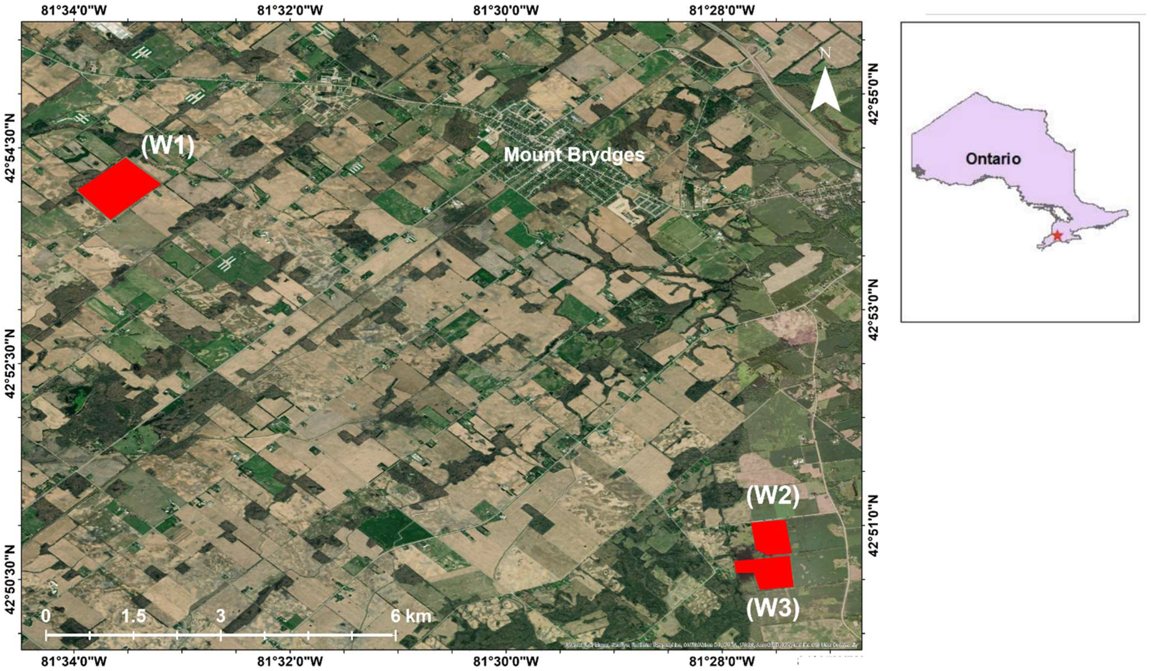
With better management of nitrogen fertilizers, not only can costs and negative environmental impacts be minimized—yield and quality can also be increased. This study aims to evaluate machine learning modelling methods with plant spectral, biophysical, and field environmental variables to predict CNW in wheat crops using UAV and satellite-based imagery. The objectives of this study include, (i) studying the relationship between the spatial variation of CNW and factors such as plant height, LAI, soil moisture, and topographic metrics within wheat fields in Southwestern Ontario using multispectral UAV—or PlanetScope—imagery; (ii) determining the optimal combination(s) of spectral variable(s), crop variables, and/or environmental conditions (soil, water, and topographic data) for wheat canopy nitrogen estimation and prediction; and (iii) evaluating the temporal variation of nitrogen estimation and prediction during the early growth stages of wheat using UAV images or PlanetScope images, and related variables.

2. Materials and Methods

2.1. Study Area and Data Collection

The study sites are in Strathroy-Caradoc, Ontario, Canada, nearby the community of Mount Brydges (Figure 1). Fieldwork was conducted during May–June 2020 with an average temperature of 22 °C and humidity averaging 73%, characteristic of southwestern Ontario’s humid continental climate zone. The sites are in a predominantly agricultural area about 25 km west of London, Ontario’s urban center.

In southwestern Ontario, winter wheat is planted in autumn for germination, lying dormant during winter and resuming growth in spring. This study’s wheat fields’ cultivar was “Soft Red Winter Wheat”, which was planted in mid-October 2019, began sprouting mid-April 2020, and was harvested in early August. The three fields labelled W1, W2, and W3 are sized at 48, 21, and 27 hectares, respectively. Beginning in early May, sampling was conducted every 7–8 days for a total of five sample dates to capture significant growth stages of the crop (

Table 1. Summary of fieldwork data acquisitions.

Fieldwork Date	Air Temperature (°C)	BBCH * Growth Stage
5 May	17	22–24
12 May	12	23–26
20 May	14	30–32
27 May	21	39–41
4 June	23	52–58

* Biologische Bundesanstalt, Bundessortenamt, and CHemische Industrie Scale.

). Wheat growth stages were recorded following the Biologische Bundesanstalt, Bundessortenamt, and CHemische Industrie (BBCH) scale [32]. The data acquired for this study encompassed the wheat crop’s growth period from leaf development up to and including inflorescence emergence (BBCH 10 to 59) for nitrogen estimation. The early stages of growth before flowering are especially important as fertilizers applied then have better nitrogen use efficiency and yield response [4,33]. Fertilizer can be applied during autumn planting, but lower probability of rainfall also decreases the amount of N from moving into the soil. Fertilizer left above soil during winter will not penetrate and may move during spring snowmelt. During later growth stages (BBCH 60+) from fruit development to ripening, root N uptake slows down as the plants translocate N from vegetation to grains and excess fertilizer can leach from the field [34].

Prior to sample point selection, a DJI Phantom 4 Real-Time Kinematics (RTK) UAV was flown over the bare soil of the fields. The UAV connected to an RTK global navigation satellite system (GNSS) base station acquired images with positioning metadata at 1.5 cm vertical and 1 cm horizontal positioning accuracy. These images were mosaicked to create a digital elevation model (DEM) GeoTiff image. The DEM was imported into Google Earth and 16 sample points were selected for each field based on the variation of elevation and coverage of representative areas (Figure 2). Considering the crop rows were planted northwest–southwest for field W1 and north–south for fields W2 and W3, the sampling pattern followed the row directions for navigation efficiency. The sample points were placed in a four-by-four grid, spaced 60 m from one another. A minimum distance of 50 m from roads was used to reduce possible effects of transportation pollution. From Google Earth, the points were exported to a KML file and downloaded onto mobile devices. On the first fieldwork date, the KML file was used to navigate to the pre-determined sample points and red flags were placed for accurate positioning in following fieldwork sessions.

To measure the biomass at each sampling point, a square guide made of plastic tubing of 50 cm × 50 cm was placed around a patch of wheat. The plants within the guide were destructively collected by cutting at the stem base above ground, then placed in paper bags. The average distance between rows was 17 cm, and mostly three rows of wheat would be collected from the 0.25 m² biomass block. On the same day following fieldwork collection, the fresh biomass was weighed in grams then fully dried in an oven at 60 °C for 48 h. Dry biomass was weighed before being sent to A&L Canada Laboratories for plant analysis. The biomass was ground into a fine powder able to pass through a 1 mm sieve before being used in the Laboratory Equipment Company (LECO) FP628 nitrogen combustion method to obtain the leaf N content percentages [35].

Six measurements of plant height in centimeters were taken around each sampling point within a 1 m² block on every fieldwork date, and an average height was calculated. Six measurements of soil moisture were collected within a 1 m² block around the sampling point using an ML3 ThetaProbe (Delta-T Devices Ltd., Burwell, Cambridge, UK) and averaged [36]. Plant phenology was recorded at each sample point using the BBCH scale to determine growth stage during data collections.

The leaf area index (LAI) was measured non-destructively using a LAI-2200C Plant Canopy Analyzer (Li-Cor, Inc., Lincoln, NE, USA) [37]. Following manufacturer recommendations, five measurements were taken along the row at each sample point during clear skies or uniform overcast conditions. Files from the device were transferred to and processed with the Li-Cor software File Viewer FV2200. Processing options include scattering correction based on the field conditions, and output text files with final LAI measurements.

2.2. UAV Imagery

In this study, the two UAVs used were a Da-Jiang Innovations (DJI) (DJI, Shenzhen, China) Matrice 100 and a DJI Phantom 4 RTK [38]. The DJI Phantom 4 was flown at 30 m altitude as per the manufacturer’s recommendations regarding the visual sensor system’s optimal performance and connection to the RTK GNSS base station. The RGB image resolution was 0.9 × 0.9 cm and capture was set to 80% side and 80% front image overlap. A fine resolution, typically < 10 cm, and high image overlap ensure a greater chance of successful image mosaicking as crop canopies densify during a growing season [27].

The DJI Matrice 100 carried a MicaSense RedEdge (MicaSense Inc., Seattle, WA, USA) narrowband multispectral camera including the following bands ordered by increasing wavelength: (1) blue, (2) green, (3), red, (4) red-edge, and (5) near-infrared (NIR) (

Table 2. Spectral characteristics of the five MicaSense bands.

Band	Name	Band Range (nm)	Centre Wavelength (nm)	Bandwidth (nm)
1	Blue	465–485	475	20
2	Green	550–570	560	20
3	Red	663–673	668	10
4	Red-Edge	712–722	717	10
5	NIR	820–860	840	40

) [39]. Image acquisition was conducted on the same dates as ground fieldwork before biomass collection. For the fieldwork conducted during the week of 27 May, the weather conditions were characterized by strong winds and sudden rain showers, so the UAV was flown on different dates between 26 May and 29 May for each field whenever the weather was suitable.

The flight plans for each field were made in the Pix4D software suite “Pix4Dcapture” app (Pix4D S.A., Prilly, Switzerland) to cover entire fields in a zigzag pattern [40]. Pix4Dcapture includes the function of adding custom UAV and sensor properties to calculate the flight plan’s estimated total time, battery usage, and image resolution at the plan’s designated altitude. The flight altitude for each field’s plan was set at 60 m, as >60 m wind and gust conditions were usually greater than the UAV manufacturer recommendations. Based on the MicaSense camera’s specifications, the resulting image resolution was 4 cm × 4 cm with capture set to 80% side and 80% front overlap. Unfortunately, images for field W3 on 5 May and field W1 on 27 May were corrupted and unusable for further processing.

2.3. UAV Image Processing

UAV image processing followed the flowchart of Figure 3. The DJI Phantom 4 RTK images taken in April over each field’s bare soil were mosaicked in Pix4Dmapper software to generate a DEM GeoTiff. Using the System for Automated Geoscientific Analysis (SAGA), a free, open-source spatial data analysis software package, topographic metrics were computed from the DEM [41]. Using the “Terrain Analysis—Morphometry” tool, the metrics generated include slope, aspect, profile curvature, and plan curvature. Creating topographic wetness indices (TWI) required several steps. First, using the “Terrain Analysis—Hydrology” tool, a flow accumulation layer of the field was created. Using the “Flow Width and Specific Catchment Areas (SCA)” tool, two SCAs were created using different algorithms: Deterministic 8 and Multiple Flow Direction. The “Topographic Wetness Index (TWI)” tool was then used to create two maps, TWI #1 and TWI #2, based on the respective algorithm SCAs. The final topographic metrics were exported as GeoTiff files.

MicaSense camera multispectral images were processed in Pix4Dmapper to create an orthomosaic image per band with 4 cm × 4 cm resolution. An important step in producing a high-quality final image is radiometric calibration considering the sensor influence and scene illumination of the UAV flight. Prior to each flight over a field, the MicaSense camera was positioned above a MicaSense Calibrated Reflectance Panel to take a minimum of five white reference images for each band. From the Exchangeable Image File Format (EXIF) metadata of the images, Pix4Dmapper can read the sensor settings, properties, and geolocation at the time the images were taken. Before starting the mosaic processing, setting options include inputting the white reference images and manufacturer-provided panel reflectance values to calibrate and correct image reflectance for each of the bands. Then, Pix4Dmapper uses the Structure from Motion (SfM) algorithm to correct image perspectives and recognize where to stitch images together [22]. The high image overlap parameters set in the flight plan enable the software to recognize greater, similar areas of each image for a higher chance of mosaic success. Pix4Dmapper processing options include georeferencing with ground control points (GCP) to improve the absolute location accuracy. Following Pix4D’s recommended number of five GCPs, black and white checkered boards were placed around the wheat fields and their coordinates recorded using a Global Positioning System (GPS) connected to the RTK. The output orthomosaic images are GeoTiff files with reflectance values for each MicaSense band.

2.4. Satellite Imagery

In this study, PlanetScope satellite imagery was acquired from Planet Labs Inc. through submission and acceptance of the project proposal. Revisit times are almost daily worldwide with resampled spatial resolution of 3 m × 3 m. The image products available for this study were from the third-generation sensors, Dove-R, with four bands ordered by increasing wavelength: (1) blue, (2) green, (3) red, (4) NIR (

Table 3. Spectral characteristics of the PlanetScope Dove-R sensors.

Band	Name	Band Range (nm)	Centre Wavelength (nm)	Bandwidth (nm)
1	Blue	464–517	491	53
2	Green	547–585	566	38
3	Red	650–682	667	32
4	NIR	846–888	867	42

). The product scenes were approximately 25 km × 23 km^, and in the case of the three study fields, all were in one image. Five satellite images were downloaded, matching the capture dates with the ground data collection dates to maintain consistency with the plant physiology and field conditions. The images were available for download as GeoTiff surface reflectance assets, orthorectified and radiometrically corrected based on the atmospheric conditions of the specific ground locations. In ArcGIS, the large scenes were cropped to smaller images of each study field for subsequent processing.

2.5. Vegetation Indices

MicaSense and PlanetScope reflectance images of each of their respective bands were exported into ArcGIS to extract crop canopy reflectance values at the sample points. With the “Raster Calculator” tool in PCI Geomatica Banff, the images were used to compute the VIs listed in

Table 4. Vegetation indices used in the study.

Index 1	Formula 2	Authors
BNDVI	(NIR − BLUE)/(NIR + BLUE)	Wang et al. [44]
CI_RE	(NIR/REDEDGE) − 1	Gitelson et al. [45]
ISR	RED/NIR	Fernandes et al. [46]
MSR	$\frac{\left(\mathrm{NIR}/\mathrm{RED}\right)-1}{\sqrt{\frac{\mathrm{NIR}}{\mathrm{RED}}+1}}$	Chen [47]
MTVI2	$\frac{1.8\left(\mathrm{NIR}-\mathrm{GREEN}\right)-3.75\left(\mathrm{RED}-\mathrm{GREEN}\right)}{\sqrt{{\left(2\mathrm{NIR}+1\right)}^2-6\left(\mathrm{NIR}-5\sqrt{\mathrm{RED}}\right)}-0.5}$	Bagheri et al. [48]
NDRE	(NIR − REDEDGE)/(NIR + REDEDGE)	Gitelson and Merzyak [49]
NDVI	(NIR − RED)/(NIR + RED)	Rouse et al. [50]
OSAVI	1.6[(NIR − RED)/(NIR + RED + 0.16)]	Rondeaux, Steven, and Baret [51]
RDVI	$\frac{\mathrm{NIR}-\mathrm{RED}}{\sqrt{\mathrm{NIR}+\mathrm{RED}}}$	Roujean and Breon [52]
RGBVI	$\left({\mathrm{GREEN}}^2-\mathrm{BLUE}\ast \mathrm{RED}\right)/\left({\mathrm{GREEN}}^2+\mathrm{BLUE}\ast \mathrm{RED}\right)$	Bendig et al. [53]
RVI	NIR/RED	Jordan [54]
RVI2	NIR/REDEDGE	Kanke et al. [55]
WDRVI	$(0.2*\mathrm{NIR}-\mathrm{RED})/(0.2*\mathrm{NIR}+\mathrm{RED})$	Gitelson [56]
VDVI	$\frac{\left(2\ast \mathrm{GREEN}-\mathrm{RED}-\mathrm{BLUE}\right)}{\left(2\ast \mathrm{GREEN}+\mathrm{RED}+\mathrm{BLUE}\right)}$	Fuentes et al. [57]

¹ Vegetation index abbreviations: BNDVI = blue normalized difference vegetation index; CI_RE = chlorophyll index red edge; ISR = infrared simple ratio; MSR = modified simple ratio; MTVI2 = modified triangular vegetation index; NDRE = normalized difference vegetation index; NDVI = normalized difference vegetation index; OSAVI = optimized soil adjusted vegetation index; RDVI = renormalized difference vegetation index; RGBVI = red green blue vegetation index; RVI = ratio vegetation index; WDRVI = wide dynamic range vegetation index; VDVI = visible band difference vegetation index. ² Formula variables: BLUE = blue reflectance; GREEN = green reflectance; RED = red reflectance; REDEDGE = red edge reflectance; NIR = near-infrared reflectance.

and exported as GeoTiff files. Using ArcGIS, the VI layer values were extracted at each sample point. As MicaSense has a red-edge band, the following three indices were included specifically for the UAV-data modelling: the chlorophyll index red-edge (CI_RE), the normalized difference vegetation index (NDRE), and the ratio vegetation index #2 (RVI2). VIs have been extensively studied for the purpose of crop monitoring and biophysical estimation, such as the normalized difference vegetation index (NDVI) [12,42]. VIs developed for chlorophyll estimation have been found to be related to plant nitrogen content as the photosynthetic enzyme, rubisco, encompasses the largest proportion of nitrogen in leaves [4]. Chlorophyll reflects green and NIR radiation and absorbs more than 70% of blue and red radiation [43].

2.6. Canopy Nitrogen Weight Modelling

CNW was calculated using the following method [58]:

$$CNW=LNC\times W_d$$

(1)

where CNW is the canopy nitrogen weight (g/m²), LNC is the leaf nitrogen content (%), and W_d is the dry biomass weight (g/m²). CNW assumes the plants collected for biomass around the sample point, within the 0.25 m² block, have the same amount of nitrogen. The total biomass per area was used as the dry biomass of wheat plants at early growth stages (BBCH < 60) since the leaves constitute most of the plant weight. Compared to other biophysical parameters such as plant nitrate content and plant nitrogen concentration (%), CNW has been found to have greater correlation with spectral data [28].

RF is an ensemble learning method suited for the classification or regression of large, nonparametric datasets. Training data are randomly selected from the dataset based on a user-defined percentage; commonly, 70% of a dataset is used to train a model. From the training data, many decision trees are generated by the algorithm to determine the variables’ importance in the regression. Decision trees split at nodes depending on the independent variable that contributes most to the dependent variable. The validation data are the remainder of the dataset that is not used in training, and the average output from decision trees is used to evaluate the model’s performance. Advantages of RF include quick computation, no overfitting from training data, and high performance in studies [29].

Support Vector Machines (SVM) are supervised learning algorithms used for classification and regression. SVR uses a decision boundary, known as a hyperplane, to split classes of training data based on data characteristics. The data points closest to either side of the hyperplane are known as support vectors, used as training samples to determine the optimal hyperplane position from the midpoint of the margin. SVR performs modelling in a high-dimensional space. SVR uses a kernel trick (i.e., the Radial Basis Kernel) for nonlinear data, placing the data in a dimensional space to separate into groups based on radial distance between data points. SVR has advantages over simple linear regression models, as its flexibility with nonparametric data has better modelling capabilities [59]. The modelling for this study was written in the R programming language using R Studio (Version 4.0.3), an open-source and free Integrated Development Environment (IDE) [60]. For RF, the “randomForest” package was used, and for SVR, the “e1071” package was used.

Modelling was performed separately for MicaSense-based and PlanetScope-based sensor variables for comparison of UAV and PlanetScope data results. The MicaSense models used all five MicaSense bands, all 14 VIs listed in Table 1, plant height, LAI, soil moisture, and topographic metrics, and the dependent variable was the CNW. The PlanetScope models used all four PlanetScope bands, 11 VIs listed in Table 1 not including the red-edge based indices (CI_RE, NDRE, RVI2), plant height, LAI, soil moisture, and topographic metrics, and the dependent variable was the CNW. Measurements of variables at each sample point were averaged to a 1 m² scale. Datasets were randomly divided into 70% training set and 30% validation set. The quality of the models was assessed using the coefficient of determination (R²) and the Root Mean Square Error (RMSE), calculated using Equations (2) and (3), respectively [61]:

$$R^2=1-\frac{{\displaystyle \sum }{(y_i-{\widehat{y}}_i)}^2}{{\displaystyle \sum }{(y_i-{\overline{y}}_i)}^2}$$

(2)

where y_i is the observed value, $\widehat{y}$_i is the predicted value, and $\overline{y}$ is the mean of the observed values of the dataset; and:

$$RMSE=\frac{{{\displaystyle \sum }}_{i=1}^n{\left({\widehat{y}}_i-y_i\right)}^2}{n}$$

(3)

where $\widehat{y}$_i is the predicted CNW value (g/m²), y_i is the observed CNW value (g/m²), n is the number of observations, and i is the index of summation in increments of one.

3. Results

3.1. Nitrogen Statistics

Overall, the canopy N weight for the wheat fields increased in variation during the fieldwork season (Figure 4). There was a slight decrease in canopy N weight from 6 to 12 May, likely due to a period of several days of continuous rainfall between samplings. Rainfall can lead to leaching of soil N from areas around plant roots, in this case reducing plant N utilization while the biomass continued to increase [62,63]. After 12 May, the farmer applied fertilizer to the wheat field once before 20 May and, consequently, the canopy N weight increased during the following weeks. There was an outlier from a sample point on 20 May, which was removed from the dataset for modelling.

3.2. Soil Statistics

A VitTellus soil health analysis [64] was conducted on the study fields, producing the following mean values: soil nitrate-nitrogen of 46.81 ppm, mineralizable nitrogen of 29.17 ppm, and water-extracted soil nitrate of 44.38 ppm. A&L Canada Soil Health Index ratings were in the “Good-High” category, and the soil textural class for the fields was predominantly sandy loam.

3.3. Regression Models with All Parameters

3.3.1. UAV Regression Models

For the UAV regression models, the first modelling step used all 28 variables including: the five MicaSense band reflectances, 14 VIs, plant height, soil moisture, LAI, topographic slope, aspect, profile curvature, plan curvature, TWI #1, and TWI #2. Single-date and combinations of multi-date datasets were tested to evaluate the temporal effect on models. A proportion of 70% of each dataset was used to calibrate the RF and SVR models, before the remaining 30% was used for validation. From the calibrated models (

Table 5. Statistics for the calibration of the UAV canopy nitrogen models with 28 variables as a function of the date and modelling approach (RF or SVR) ¹.

Date	Model	R2	RMSE (g/m2)	(n)
5 May	RF	0.91	0.51	22
	SVR	0.78	0.70	22
12 May	RF	0.92	0.31	33
	SVR	0.80	0.46	33
20 May	RF	0.85	1.12	33
	SVR	0.58	1.89	33
27 May	RF	0.95	1.63	22
	SVR	0.84	2.43	22
4 June	RF	0.91	2.36	33
	SVR	0.81	3.00	33
5 and 12 May	RF	0.95	0.55	56
	SVR	0.77	0.84	56
12 and 20 May	RF	0.94	0.88	67
	SVR	0.80	1.53	67
20 and 27 May	RF	0.95	1.37	56
	SVR	0.79	2.87	56
27 May, 4 June	RF	0.95	2.28	56
	SVR	0.76	3.86	56
5, 12, and 20 May	RF	0.92	0.87	89
	SVR	0.79	1.40	89
12, 20, and 27 May	RF	0.96	1.07	89
	SVR	0.87	2.07	89
20 and 27 May, 4 June	RF	0.97	1.76	89
	SVR	0.85	3.79	89

¹ All models are significant at p-value < 0.001.

), RF had better performance in comparison to SVR; specifically, it had higher R² and lower RMSE values overall. The top model performance was that of RF with the combination of 12, 20, and 27 May resulting in an R² of 0.96 and an RMSE of 1.07 g/m². Although the 20/27 May and 4 June model had a slightly higher R² of 0.97, the RMSE was considerably greater at 1.76 g/m². Of the RF and SVR models, that of 20 May had the lowest performance. Of the SVR models, 12, 20, and 27 May model had the best performance with an R² of 0.87 and an RMSE of 2.07 g/m².

The UAV models were then applied to the validation datasets (

Table 6. Statistics for the validation of the UAV canopy nitrogen models with 28 variables as a function of the date and modelling approach (RF or SVR).

Date	Model	R2	p-Value 1	RMSE (g/m2)	(n)
5 May	RF	0.18	NS	0.71	10
	SVR	0.06	NS	0.71	10
12 May	RF	0.07	NS	0.95	15
	SVR	0.14	0.1	0.79	15
20 May	RF	0.05	NS	2.28	15
	SVR	0.18	0.1	2.14	15
27 May	RF	0.25	0.1	4.35	10
	SVR	0.03	NS	5.05	10
4 June	RF	0.20	0.1	4.35	15
	SVR	0.06	NS	5.66	15
5 and 12 May	RF	0.41	<0.001	0.99	24
	SVR	0.52	<0.001	0.81	24
12 and 20 May	RF	0.66	<0.001	1.72	29
	SVR	0.71	<0.001	1.56	29
20 and 27 May	RF	0.67	<0.001	2.26	24
	SVR	0.55	<0.001	2.38	24
27 May, 4 June	RF	0.45	<0.001	5.80	24
	SVR	0.30	0.001	6.44	24
5, 12, and 20 May	RF	0.37	<0.001	1.58	39
	SVR	0.52	<0.001	1.32	39
12, 20, and 27 May	RF	0.74	<0.001	2.76	39
	SVR	0.61	<0.001	3.50	39
20 and 27 May, 4 June	RF	0.74	<0.001	4.12	39
	SVR	0.71	<0.001	4.46	39

¹ NS = non-significant.

). All single date models for RF and SVR had low performance. This was likely due to the small number of sample point data from single date sets resulting in the calibration model not encompassing normal field data variation. The top performing model was RF with the 12, 20, and 27 May data, resulting in an R² of 0.74 and an RMSE of 2.76 g/m². Overall, RF had better performance than SVR and multi-date models had better performance than single-date models.

3.3.2. PlanetScope Regression Models

For the PlanetScope regression models, 24 variables were used in the first step, including: the four PlanetScope band reflectances, 11 VIs, plant height, soil moisture, LAI, topographic slop, aspect, profile curvature, plan curvature, TWI #1, and TWI #2. To test the temporal effects on the models, single-date and multi-date dataset combinations were used. Taking 70% of the dataset to calibrate the RF and SVR models, overall RF had better performance to SVR with higher R² and lower RMSE values (

Table 7. Statistics for the calibration of the PlanetScope canopy nitrogen models with 24 variables as a function of the date and the modelling approach (RF or SVR) ¹.

Date	Model	R2	RMSE (g/m2)	(n)
5 May	RF	0.94	0.40	33
	SVR	0.82	0.60	33
12 May	RF	0.92	0.30	33
	SVR	0.71	0.49	33
20 May	RF	0.85	1.23	33
	SVR	0.52	2.03	33
27 May	RF	0.90	1.89	33
	SVR	0.60	3.41	33
4 June	RF	0.91	2.23	33
	SVR	0.70	3.80	33
5 and 12 May	RF	0.95	0.55	67
	SVR	0.76	0.83	67
12 and 20 May	RF	0.94	0.78	67
	SVR	0.78	1.48	67
20 and 27 May	RF	0.94	1.27	67
	SVR	0.75	2.57	67
27 May, 4 June	RF	0.94	1.93	67
	SVR	0.74	3.87	67
5, 12, and 20 May	RF	0.93	0.75	100
	SVR	0.74	1.34	100
12, 20, and 27 May	RF	0.96	1.10	100
	SVR	0.87	2.12	100
20 and 27 May, 4 June	RF	0.95	1.87	100
	SVR	0.83	3.68	100

¹ All models are significant at p-value < 0.001.

). Of all models, RF with the combination of the 12, 20, and 27 May data had best performance with an R² of 0.96 and an RMSE of 1.10 g/m². Of the SVR models alone, the 12, 20, and 27 May model had the highest performance with an R² of 0.87 and an RMSE of 2.12 g/m².

Next, the PlanetScope models were applied to the remaining 30% of datasets for validation (

Table 8. Statistics for the validation of the PlanetScope canopy nitrogen models with 24 variables as a function of the date and the modelling approach (RF or SVR).

Date	Model	R2	p-Value 1	RMSE (g/m2)	(n)
5 May	RF	0.44	0.001	0.92	15
	SVR	0.51	0.001	0.90	15
12 May	RF	0.45	0.001	0.62	15
	SVR	0.78	<0.001	0.53	15
20 May	RF	0.05	NS	2.24	15
	SVR	0.38	0.001	1.90	15
27 May	RF	0.63	<0.001	2.84	15
	SVR	0.50	0.001	3.40	15
4 June	RF	0.07	NS	6.24	15
	SVR	0.05	NS	5.54	15
5 and 12 May	RF	0.44	<0.001	1.06	29
	SVR	0.29	0.001	1.08	29
12 and 20 May	RF	0.79	<0.001	1.37	29
	SVR	0.71	<0.001	1.03	29
20 and 27 May	RF	0.63	<0.001	3.24	29
	SVR	0.50	<0.001	3.79	29
27 May, 4 June	RF	0.63	<0.001	4.77	29
	SVR	0.63	<0.001	4.94	29
5, 12, and 20 May	RF	0.50	<0.001	1.73	44
	SVR	0.68	<0.001	1.43	44
12, 20, and 27 May	RF	0.83	<0.001	1.77	44
	SVR	0.67	<0.001	3.16	44
20 and 27 May, 4 June	RF	0.75	<0.001	3.64	44
	SVR	0.74	<0.001	4.59	44

¹ NS = non-significant.

). Of all the models, single-date 20 May and 4 June had very low performance for both RF and SVR. Comparing all RF and SVR models, RF usually had better performance than SVR except in the single date models of 5 May, 12 May, and 20 May, and the multi-date model with the three dates combined. The top performing model was RF with 12, 20, and 27 May data resulting in an R² of 0.83 and an RMSE of 1.77 g/m².

3.4. Variable Importance Plots

The top performing UAV and PlanetScope regression models with all variables were both from RF and were multi-date combinations of the 12, 20, and 27 May datasets. Modelling of RF in RStudio can be visualized with a variable importance plot using the “varImpPlot()” function. The higher a variable’s IncNodePurity value is, the more important the explanatory variable is in the prediction of CNW. In the UAV model plot (Figure 5) with 28 variables, plant height was by far the most important predictor, followed by LAI. Red-edge VIs (NDRE, RVI2, CI_RE) were the third, fourth, and sixth most important predictor variables, respectively. Of the MicaSense band reflectances, NIR was the most important. Soil moisture also appeared to be among the top group of important variables with a greater difference in IncNodePurity compared to the other variables in the plot below. Of the topographic metrics, TWI #2 and TWI #1 held more importance than the rest.

The satellite RF regression model plot with 24 variables indicates height as the most important predictor for CNW (Figure 6). Of the four PlanetScope band reflectances, the blue band was most important and second-most important overall of all variables, followed closely by LAI. Overall, VIs and PlanetScope bands were among the most important variables, while topographic metrics and soil moisture were the least important.

3.5. Regression Models with Selected Parameters

3.5.1. UAV Regression Models

From the variable importance plot of the best-performing UAV regression model using 12, 20, and 27 May data, combinations of variables were tested in the RF and SVR models. Evaluating based on thresholds of variable importance, as shown in Figure 5, we selected variables for the top 7, 8, 9, 13, and 16 variable groups. An additional group containing only MicaSense band reflectances and VIs was included for comparison as common modelling approaches in other studies use only spectral variables [3]. Furthermore, 70% of each variable group dataset was used for model calibration (

Table 9. Statistics for the calibration of the canopy nitrogen model with 12, 20, and 27 May MicaSense data and different combinations of variables (n = 89) ¹.

Input Variables	Model	Number of Variables	R2	RMSE (g/m2)
Spectral-only: All VIs & 5 MicaSense bands	RF	19	0.92	1.50
	SVR	19	0.66	3.04
Top 7: Height, LAI, NDRE, RVI2, BNDVI, CI_RE, NIR	RF	7	0.96	1.15
	SVR	7	0.86	2.05
Top 8: Top 7 + Soil Moisture	RF	8	0.96	1.12
	SVR	8	0.85	2.21
Top 9: Top 8 + RDVI	RF	9	0.96	1.07
	SVR	9	0.85	2.13
Top 13: Top 9 + OSAVI, WDRVI, VDVI, RGBVI	RF	13	0.96	1.07
	SVR	13	0.85	2.10
Top 16: Top 13 + ISR, RVI, MTVI2	RF	16	0.96	1.11
	SVR	16	0.85	2.11

¹ All models are significant at p-value < 0.001.

). Overall, RF had better performance than SVR in terms of higher R² and lower RMSE values. All variable group models using RF had a high R² of 0.96 except for the spectral-only variable group with lower R². RF models’ RMSE values were also very close, within <0.10 g/m² difference, the lowest being the top 9 and top 13 variable groups at 1.07 g/m². Again, the RF spectral-only variable group had poorer performance in comparison to other RF models, as its RMSE value was significantly higher. The SVR spectral-only variable group performed poorly compared to all the other SVR models. Of the SVR models, the top 7 variable group had the best performance with an R² of 0.86 and an RMSE of 2.05 g/m². The top 8, 9, 13, and 16 variable SVR models had only slightly lower R² and higher RMSE values compared to the best SVR model.

The calibrated models were applied to the remaining 30% of datasets for validation (

Table 10. Statistics for the validation of the canopy nitrogen model with 12, 20, and 27 May MicaSense data and different combinations of variables (n = 39) ¹.

Input Variables	Model	Number of Variables	R2	RMSE (g/m2)
Spectral-only: All VIs & 5 MicaSense bands	RF	19	0.50	3.83
	SVR	19	0.48	3.87
Top 7: Height, LAI, NDRE, RVI2, BNDVI, CI_RE, NIR	RF	7	0.73	2.81
	SVR	7	0.80	2.62
Top 8: Top 7 + Soil Moisture	RF	8	0.73	2.78
	SVR	8	0.78	2.82
Top 9: Top 8 + RDVI	RF	9	0.74	2.77
	SVR	9	0.77	2.80
Top 13: Top 9 + OSAVI, WDRVI, VDVI, RGBVI	RF	13	0.75	2.72
	SVR	13	0.77	2.76
Top 16: Top 13 + ISR, RVI, MTVI2	RF	16	0.74	2.73
	SVR	16	0.76	2.81

¹ All models are significant at p-value < 0.001.

). In the validation models, SVR had better performance than RF except for the spectral-only model. The best-performing model was SVR with the top seven variables, resulting in an R² of 0.80 and an RMSE of 2.62 g/m². Compared to the best model, other SVR models had close performance, but as more variables were added, the R² had lower values.

3.5.2. PlanetScope Regression Models

For the UAV regression models using single and multi-date datasets, the best-performing combination was the model using the 12, 20, and 27 May data with RF. Evaluating based on thresholds of variable importance, as shown in Figure 6, the selected variable groups for further model testing included the top 6, 10, 13, 17, and a group containing only PlanetScope band reflectances and VIs. A proportion of 70% of each variable group dataset was used for model calibration (

Table 11. Statistics for the calibration of the PlanetScope canopy nitrogen model with 12, 20, and 27 May data and different combinations of variables (n = 100) ¹.

Input Variables	Model	Number of Variables	R2	RMSE (g/m2)
Spectral-only: VIs & 4 PlanetScope bands	RF	15	0.96	1.21
	SVR	15	0.77	2.81
Top 6: Height, BLUE, LAI, BNDVI, RDVI, OSAVI	RF	6	0.96	1.18
	SVR	6	0.84	2.31
Top 10: Top 6 + ISR, MTVI2, NIR, RED	RF	10	0.96	1.20
	SVR	10	0.84	2.35
Top 13: Top 10 + MSR, GREEN, RBGVI	RF	13	0.96	1.21
	SVR	13	0.81	2.45
Top 17: Top 13 + RVI, VDVI, NDVI, WDRVI	RF	17	0.96	1.26
	SVR	17	0.82	2.63

¹ All models are significant at p-value <0.001.

). Of the calibration models, all RF models had the same high R² value with low RMSE compared to all SVR models. The best model performance was RF with the top six variables, with an R² at 0.96 and an RMSE 1.18 g/m². For the SVR models, the best-performing was the combination of the top six variables, resulting in an R² of 0.84 and an RMSE of 2.31 g/m². From the calibration models, the spectral-only SVR model had the poorest performance with an R² of 0.77 and an RMSE of 2.81 g/m².

The remaining 30% of variable datasets were used for the validation models (

Table 12. Statistics for the validation of the PlanetScope canopy nitrogen model with 12, 20, and 27 May data and different combinations of variables (n = 44) ¹.

Input Variables	Model	Number of Variables	R2	RMSE (g/m2)
Spectral-only: VIs & 4 PlanetScope bands	RF	15	0.66	3.20
	SVR	15	0.69	3.09
Top 6: Height, BLUE, LAI, BNDVI, RDVI, OSAVI	RF	6	0.72	2.90
	SVR	6	0.85	2.17
Top 10: Top 6 + ISR, MTVI2, NIR, RED	RF	10	0.83	2.16
	SVR	10	0.84	2.06
Top 13: Top 10 + MSR, GREEN, RBGVI	RF	13	0.87	2.20
	SVR	13	0.86	2.39
Top 17: Top 13 + RVI, VDVI, NDVI, WDRVI	RF	17	0.92	1.75
	SVR	17	0.91	1.85

¹ All models are significant at p-value < 0.001.

). The poorest model performances for RF and SVR were from the spectral-only variable group, resulting in the lowest R² and highest RMSE values out of all tested. SVR had better performance compared to RF in the spectral-only, top 6, and top 10 groups, but for the top 13 and top 17 groups, RF was better. The best-performing model was RF with the top 17 variables, with an R² of 0.92 and an RMSE of 1.75 g/m².

3.6. Crop Nitrogen Prediction Maps

To create the crop nitrogen prediction maps, raster layers of each variable were required. The VI raster layers were created using the raster calculator in PCI Geomatica Banff from the MicaSense band rasters mosaicked from Pix4Dmapper. To extract raster layers for height, the Phantom 4 RTK flight processed in Pix4Dmapper includes the option for a digital surface model (DSM) output. The DSM captures the natural and built features of the environment. By subtracting the DEM raster from the DSM raster pixel values using ArcGIS raster calculator, the output raster layer has the height data of the crop [65].

Generating an LAI raster layer is a more involved process. The process is based on methodology proposed by Song et al. (2020) using a simulated observation of a point cloud Multiview angle (SOPC-M) designed to obtain a 3D spatial distribution of vegetation and bare ground points to calculate the gap fraction, followed by the crop’s effective LAI (LAIe), from a UAV-based 3D point cloud dataset [66]. In ArcGIS, the point data layer was converted to a raster layer using the “Point to Raster” conversion tool to a 2 m × 2 m resolution. From the linear regression equation, the digital hemispherical photography (DHP) LAIe could be calculated using the ArcGIS raster layer to create the final LAI raster used in the model. For field W3, the LAI layer processing area error unfortunately only covered 12 of the 16 sample points; thus, the final map produced did not cover all sample points.

Prior to running the regression models in R, the raster layers needed to have the same resolution and extent for the functions to stack them. All raster layers were run through the ArcGIS “Resample” tool to 1 m × 1 m resolution, as the CNW variable is based on a 1 m² area. Resampling was conducted with the bilinear technique, which is a bilinear interpolation and determines the new value of a cell based on a weighted distance average of the four nearest input cell centers. As the LAI raster extent was the smallest of all rasters, it was used as the output extent reference layer for the ArcGIS “Clip Raster” tool with the selected option to maintain clipping extent. The columns and rows of the output raster were adjusted, and the pixels were resampled to match the reference layer exactly. Next, the ArcGIS “Extract by Mask” tool was used to extract the cell values specifically where the LAI raster extent pixels held values greater than zero. Thus, each variable layer was prepared for the R modelling.

For the UAV best-performing model, SVR with the top seven variables included height, LAI, NDRE, RVI2, BNDVI, CI_RE, and NIR. In R, the “raster”, “rgdal”, and “rasterVis” libraries were used to generate the final prediction map outputs. The variable raster layers were stacked using the “raster::stack” function, and the “raster::predict” tool was used with the selected UAV-based SVR model using the top seven variables. The resulting prediction rasters for each field were exported as GeoTiff files into ArcGIS to create the final prediction maps with 1 m × 1 m resolution (Figure 7). The low and high CNW areas are displayed in red and green, respectively, for distinct contrast between the nitrogen levels. From the prediction rasters, the predicted CNW values around each sample point were extracted and compared to the measured values in-field. The resulting RMSE values for W1, W2, and W3 were 4.27, 2.32, and 3.08 g/m², respectively.

The best-performing satellite model used RF with the top 17 variables: height, LAI, 11 VIs, and the four PlanetScope bands. Following the same processing steps as the UAV-based model, the satellite variable raster images were processed to have the same extent and 1 m × 1 m resolution. As the satellite images began with 3 m × 3 m resolution, much larger compared to the UAV images, the resulting raster layers had a smoothed appearance. The final prediction rasters for each field are displayed as maps in Figure 8 with 1 m × 1 m resolution. From the prediction rasters, the predicted CNW values around each sample point were extracted and compared to the measured values in-field. The resulting RMSE values for W1, W2, and W3 were 3.12, 1.79, and 3.08 g/m², respectively.

Comparing the maps in Figure 7 and Figure 8, it can be seen that there were differences in the spatial distribution and values of CNW. It appears that the UAV maps show more areas with low canopy nitrogen weight, while PlanetScope shows more areas with high CNW. This is likely due to the resampling method, as the UAV’s centimeter-level image resolution includes spectral data of the visible soil between crop rows, while for PlanetScope images with coarser meter-level resolution, the pixel values average towards the spectral values of the crop rather than the soil. The UAV-based nitrogen prediction maps may have lower performance compared to satellite-based maps because of the volatile weather conditions during the fieldwork conducted on the week of May 27th. The UAV was flown on different dates between May 26th and May 29th for each field whenever the weather was suitable, and the crop spectral characteristics may have changed. However, the satellite images for the three fields for May 27th were all from the same date and present a more consistent relationship with the fieldwork data.

4. Discussion

For this study, the RF and SVM regression methods were used to predict the CNW of wheat using UAV MicaSense band reflectances, PlanetScope band reflectances, selected VIs, plant height, LAI, soil moisture, and topographic metrics. The models created were grouped according to UAV-based and satellite-based data.

For the UAV RF and SVR regression models, calibration was conducted with 28 variables from single and multi-date datasets. Evaluating the validation models of each dataset, the performance of UAV single-date models was poor with R² values of, at most, 0.25 and overall non-significant results. Combining UAV multi-date data yielded better results, with the best performance from the RF three-date model of 12, 20, and 27 May resulting in an R² of 0.74 and an RMSE of 2.76 g/m². For the PlanetScope RF and SVR models, the calibration of the models used 24 variables for single and multi-date datasets. Of the validation models, the single-date models of 20 May and 4 June had the lowest performance. However, the other PlanetScope single-date models’ performances were much better overall compared to the UAV single-date models. In general, the PlanetScope multi-date models did not have significantly better results than its single-date models. The best-performing PlanetScope model was that which was based on three dates, 12, 20, and 27 May, using RF, with an R² of 0.83 and an RMSE of 1.77 g/m². Both the best UAV and best satellite models were from 12, 20, and 27 May data, during which the wheat crops were in the BBCH 23–41 growth stages, mainly defined by tillering, stem elongation, and the beginning of the booting stage. As noted by Hawkesford (2017), the application of nitrogen fertilizer during these early growth stages before flowering is most conducive to efficient nitrogen use and yield response [67]. The ability to accurately estimate the nitrogen levels of crops during early growth stages would be most beneficial for farmers.

In the RF variance importance plot of the best-performing UAV model, of all variables, plant height was the most important predictor of CNW. Song and Wang (2019) also noted that plant height is useful in estimating phenology, biomass, and yield in addition to nitrogen uptake in wheat [68]. On the plot, LAI was the second most important predictor of CNW. LAI has been used extensively in studies to successfully predict crop chlorophyll content, biomass, and yield [69,70]. The study by Zhao et al. (2014) found a significant positive relationship between LAI and differences in crop nitrogen content across wheat growth stages [71]. The gap fraction method of calculating LAI is more accurate during the earlier growth stages of a crop when the canopy is not so dense, allowing for contrast between the vegetation and soil or vegetation and sky images [68]. Among the VI’s used in the model, the red-edge VIs (NDRE, RVI2, and CI_RE) were amongst the most important. The red-edge region (680–800 nm) has been shown to encompass sharp changes in the canopy reflectance and can be used to identify important biophysical parameters of the crop. Nitrogen levels have shown the sensitivity of the red-edge region in estimating leaf chlorophyll content due to the high absorption of red radiation and high reflectance of NIR radiation [69,72]. Of the MicaSense bands individually, the NIR band was of highest importance in the model while other individual bands had little effect. Soil moisture also appeared as a variable of high importance, and subsequent variables on the plot had noticeably lower importance. Studies have noted the importance of soil moisture in soil nitrogen mineralization, crop nitrogen uptake, and utilization [73,74]. Of the topographic metrics, the topographic wetness indices were most important, while the remaining metrics had little effect.

In the RF variance importance plot of the best-performing satellite model, similar to the UAV model, plant height was the most important predictor of CNW, with LAI following closely. Interestingly, the PlanetScope blue band was the second most important variable. As the PlanetScope blue band has greater width compared to MicaSense, perhaps the wider bandwidth captured a change of canopy reflectance in the blue-edge region (480–517 nm) which was previously noted in the study by Wei et al. (2008) to be related to crop nitrogen [75]. Other PlanetScope bands in the model had varying levels of importance interspersed amongst the 11 VIs used. On the plot, other non-spectral variables of soil moisture and topographic metrics were of least importance to the model.

From the UAV-based RF variance importance plot, groups of variables were selected for testing in models. Groups of the top 7, 8, 9 13, 16, and spectral-only variables were modeled, with the group of top seven variables of the SVR model performing the best with an R² of 0.80 and an RMSE of 2.62 g/m². The top seven variables included plant height, LAI, all three red-edge VIs, BNDVI, and the MicaSense NIR band. Compared to the best models from studies by Asataoui et al. (2021), Jiang et al. (2019), and Zheng et al. (2018) using UAV-based spectral variables to estimate wheat nitrogen content, their models had lower R² values, ranging from 0.76 to 0.63, and greater RMSE values [24,26,27]. With the UAV-based best model in this study, significantly lower RMSE is a major advantage in terms of reducing the costs of nitrogen fertilizer.

The satellite-based variance importance plot was used to select variable groups for model testing including the top 6, 10, 13, 17, and spectral-only variables. The RF model group of the top 17 variables had the best performance with an R² of 0.92 and an RMSE of 1.75 g/m². The height, LAI, all four PlanetScope bands, and total 11 VIs were the variables in the best-performing model. For both the UAV and satellite best-performing selected-variable models, plant height and LAI were the only non-spectral variables. With methods for deriving the height and LAI of a wheat crop field from the UAV Phantom 4 RTK imagery, all variables in the top models can be obtained from in-situ, non-destructive, remote sensing data.

For both the UAV and satellite spectral-only variable groups, the results were poor with R² values <0.50 and significantly higher RMSE values compared to other tested variable groups. This is consistent with the studies by Astaoui et al. (2021) and Schirrmann et al. (2016), in which it was noted that, within wheat crops, UAV imagery was limited for the observation of nitrogen status but had good performance in the monitoring of biophysical parameters [27,28]. For the UAV validation spectral-only model, the RMSE dropped by 32% as compared to the best-performing top seven variable model. In the satellite validation spectral-only model, the RMSE dropped by 45% compared to the best-performing top 17 variable model.

In the final validation of canopy nitrogen models with variable combinations, the UAV SVR models mostly had greater R² values but also greater RMSE values compared to the RF models. In the UAV spectral-only variable group models, RF had better results than SVR. Considering studies with spectral-only variables for crop nitrogen models, the results are consistent, with RF yielding better nitrogen level prediction compared to SVR models [25,29,76]. Only in the UAV best-performing model of top seven variables was SVR performance better in terms of having both a higher R² value and a lower RMSE compared to RF. Of the satellite variable combination models, SVR had better performance than RF except for the top 13 and 17 variable groups. The best-performing satellite model was RF with the top 17 variable group. Although it appears difficult to determine if RF or SVR models are better when built with non-spectral and spectral variables together, ultimately the ideal result is a model which can most accurately predict canopy nitrogen in wheat. In both the UAV and satellite models with different variable combinations, the top variable groups had good overall performances. In comparison to studies with spectral-only variable models, the variable combination models in this study all had lower RMSE values. In the context of nitrogen estimation and practical application, lower RMSE (g/m²) in models is most beneficial for fertilizer management recommendations.

5. Conclusions

In this study, machine learning regression methods were tested to predict wheat CNW using UAV MicaSense band reflectances, PlanetScope band reflectances, associated VIs, plant height, LAI, soil moisture, and topographic metrics. For UAV models using 28 variables, the combination of 12, 20, and 27 May data with the RF validation model produced the best results with an R² of 0.74 and an RMSE of 2.76 g/m². From the model’s variable importance plot, the top 7, 8, 9, 13, 16, and spectral-only variable groups were tested. The best validation model used SVR with the top seven variables, which included plant height, LAI, four VIs, and the MicaSense NIR band. For the PlanetScope models using 24 variables, the best performing model was RF with 12, 20, and 27 May data resulting in an R² of 0.83 and an RMSE of 1.77 g/m². Based on the model’s variable importance plot, the top 6, 10, 13, 17, and spectral-only variable groups were tested. The validation model with the best performance was RF using the top 17 variables including height, LAI, all four PlanetScope bands, and 11 VIs.

A common limitation of in-situ agricultural models, including those developed in this study, are their empirical nature, and applicability can be limited to the dataset they are built and validated upon. Each field and growing season has different conditions and factors that affect plant growth, so models will need further testing to determine their effectiveness in precision agriculture methods. PlanetScope satellite constellation has also launched, and a third generation of sensors were introduced in 2020, known as SuperDove, with the potential to capture imagery with eight spectral bands including a red-edge band. Future work can consider further testing satellite-based nitrogen prediction models including red-edge VI variables.

References

1. Bongiovanni, R.; Lowenberg-DeBoer, J. Precision agriculture and sustainability. Precis. Agric. 2004, 5, 359–387. [Google Scholar] [CrossRef]
2. Masclaux-Daubresse, C.; Daniel-Vedele, F.; Dechorgnat, J.; Chardon, F.; Gaufichon, L.; Suzuki, A. Nitrogen uptake, assimilation, and remobilization in plants: Challenges for sustainable and productive agriculture. Ann. Bot. 2010, 105, 1141–1157. [Google Scholar] [CrossRef] [PubMed] [Green Version]
3. Sishodia, R.P.; Ray, R.L.; Singh, S.K. Applications of remote sensing in precision agriculture: A review. Remote Sens. 2020, 12, 3136. [Google Scholar] [CrossRef]
4. Marschner, H. Marschner’s Mineral Nutrition of Higher Plants, 2nd ed.; Academic Press: Adelaide, Australia, 2011. [Google Scholar]
5. Fageria, N.K. The Use of Nutrients in Crop Plants; CRC Press: New York, NY, USA, 2009. [Google Scholar]
6. Fageria, N.K.; Baligar, V.C.; Jones, C.A. Growth and Mineral Nutrition of Field Crops, 3rd ed.; CRC Press: New York, NY, USA, 2010. [Google Scholar]
7. Rabalais, N.N.; Turner, R.E.; Wiseman, W.J., Jr. Hypoxia in the Gulf of Mexico. J. Environ. Qual. 2001, 30, 320–329. [Google Scholar] [CrossRef] [PubMed]
8. Foulkes, M.J.; Slafer, G.A.; Davies, W.J.; Berry, P.M.; Sylvester-Bradley, R.; Martre, P.; Calderini, D.; Griffiths, S.; Reynolds, M.P. Raising yield potential of wheat. III. Optimizing partitioning to grain while maintaining lodging resistance. J. Exp. Bot. 2011, 62, 469–486. [Google Scholar] [CrossRef] [PubMed] [Green Version]
9. Drew, M.C.; Sisworo, E.J. Early effects of flooding on nitrogen deficiency and leaf chlorosis in barley. New Phytol. 1977, 79, 567–571. [Google Scholar] [CrossRef]
10. Si, B.; Farrell, R. Scale-dependent relationship between wheat yield and topographic indices. Soil Sci. Soc. Am. J. 2004, 68, 577–587. [Google Scholar] [CrossRef]
11. Walley, F.; Yates, T.; Van Groenigen, J.W.; Kessel, C. Relationships between soil nitrogen availability indices, yield, and nitrogen accumulation of wheat. Soil Sci. Soc. Am. J. 2002, 66, 1549–1561. [Google Scholar] [CrossRef] [Green Version]
12. Jones, H.G.; Vaughan, R.A. Remote Sensing of Vegetation: Principles, Techniques, and Applications, 1st ed.; University Press: New York, NY, USA, 2010. [Google Scholar]
13. Eitel, J.U.H.; Long, D.S.; Gessler, P.E.; Smith, A.M.S. Using in-situ measurements to evaluate the new RapidEye satellite series for prediction of wheat nitrogen status. Int. J. Remote Sens. 2007, 28, 4183–4190. [Google Scholar] [CrossRef]
14. Frels, K.; Gutteieri, M.; Joyce, B.; Leavitt, B.; Baenziger, S. Evaluating canopy spectral reflectance vegetation indices to estimate nitrogen use traits in hard winter wheat. Field Crops Res. 2018, 217, 82–92. [Google Scholar] [CrossRef]
15. Sripada, R.P.; Schmidt, J.P.; Dellinger, A.E.; Beegle, D.B. Evaluating multiple indices from a canopy reflectance sensor to estimate corn N requirements. Agron. J. 2008, 100, 1553–1561. [Google Scholar] [CrossRef]
16. Agriculture and Agri-Food Canada. An Overview of the Canadian Agriculture and Agri-Food System. Available online: https://www.agr.gc.ca/eng/canadas-agriculture-sectors/an-overview-of-the-canadian-agriculture-and-agri-food-system-2017/?id=1510326669269 (accessed on 23 February 2021).
17. Mulla, D.J. Twenty-five years of remote sensing in precision agriculture: Key advances and remaining knowledge gaps. Biosyst. Eng. 2013, 114, 358–371. [Google Scholar] [CrossRef]
18. Planet, Planet Imagery Product Specifications. Available online: https://assets.planet.com/docs/Planet_Combined_Imagery_Product_Specs_letter_screen.pdf (accessed on 20 July 2021).
19. Breunig, F.M.; Galvão, L.S.; Dalagnol, R.; Santi, A.L.; Della Flora, D.P.; Chen, S. Assessing the effect of spatial resolution on the delineation of management zones for smallholder farming in southern Brazil. Remote Sens. Appl. Soc. Environ. 2020, 19, 100325. [Google Scholar] [CrossRef]
20. Manivasagam, V.S.; Sadeh, Y.; Kaplan, G.; Bonfil, D.J.; Rozenstein, O. Studying the Feasibility of Assimilating Sentinel-2 and PlanetScope Imagery into the SAFY Crop Model to Predict Within-Field Wheat Yield. Remote Sens. 2021, 13, 2395. [Google Scholar] [CrossRef]
21. Sadeh, Y.; Zhu, X.; Dunkerley, D.; Walker, J.P.; Zhang, Y.; Rozenstein, O.; Manivasagam, V.S.; Chenu, K. Fusion of Sentinel-2 and PlanetScope time-series data into daily 3 m surface reflectance and wheat LAI monitoring. Int. J. Appl. Earth Obs. Geoinf. 2021, 96, 102260. [Google Scholar] [CrossRef]
22. Harwin, S.; Lucieer, A. Assessing the accuracy of georeferenced point clouds produced via multi-view stereopsis from unmanned aerial vehicle (UAV) imagery. Remote Sens. 2012, 4, 1573–1599. [Google Scholar] [CrossRef] [Green Version]
23. Hunt, E.R.; Hively, W.D.; Fujikawa, S.J.; Linden, D.S.; Daughtry, C.S.T.; McCarty, G.W. Acquisition of NIR-green-blue digital photographs from unmanned aircraft for crop monitoring. Remote Sens. 2010, 2, 290–305. [Google Scholar] [CrossRef] [Green Version]
24. Jiang, J.; Cai, W.; Zheng, H.; Cheng, T.; Tian, Y.; Zhu, Y.; Ehsani, R.; Hu, Y.; Niu, Q.; Gui, L.; et al. Using digital cameras on an unmanned aerial vehicle to derive optimum color vegetation indices for leaf nitrogen concentration monitoring in winter wheat. Remote Sens. 2019, 11, 2667. [Google Scholar] [CrossRef] [Green Version]
25. Liu, Y.; Cheng, T.; Zhu, Y.; Tian, Y.; Cao, W.; Yao, X.; Wang, N. Comparative analysis of vegetation indices, non-parametric and physical retrieval methods for monitoring nitrogen in wheat using UAV-based multispectral imagery. In Proceedings of the 2016 IEEE International Geoscience and Remote Sensing Symposium (IGARSS), Beijing, China, 10–15 July 2016; pp. 7362–7365. [Google Scholar] [CrossRef]
26. Zheng, H.; Li, W.; Jiang, J.; Liu, Y.; Cheng, T.; Tian, Y.; Zhu, Y.; Cao, W.; Zhang, Y.; Yao, X. A comparative assessment of different modeling algorithms for estimating leaf nitrogen content in winter wheat using multispectral images from an unmanned aerial vehicle. Remote Sens. 2018, 10, 2026. [Google Scholar] [CrossRef] [Green Version]
27. Astaoui, G.; Dadaiss, J.E.; Sebari, I.; Benmansour, S.; Mohamed, E. Mapping wheat dry matter and nitrogen content dynamics and estimation of wheat yield using UAV multispectral imagery machine learning and a variety-based approach: Case study of Morocco. AgriEngineering 2021, 3, 29–49. [Google Scholar] [CrossRef]
28. Schirrmann, M.; Giebel, A.; Gleiniger, F.; Pflanz, M.; Lentschke, J.; Dammer, K.H. Monitoring agronomic parameters of winter wheat crops with low-cost UAV imagery. Remote Sens. 2016, 8, 706. [Google Scholar] [CrossRef] [Green Version]
29. Lee, H.; Wang, J.; Leblon, B. Using linear regression, random forests, and support vector machine with unmanned aerial vehicle multispectral images to predict canopy nitrogen weight in corn. Remote Sens. 2020, 12, 2071. [Google Scholar] [CrossRef]
30. Chen, P.; Haboudane, D.; Tremblay, N.; Wang, J.; Vigneault, P.; Li, B. New spectral indicator assessing the efficiency of crop nitrogen treatment in corn and wheat. Remote Sens. Environ. 2010, 114, 1987–1997. [Google Scholar] [CrossRef]
31. Yu, J.; Wang, J.; Leblon, B. Evaluation of Soil Properties, Topographic Metrics, Plant Height, and Unmanned Aerial Vehicle Multispectral Imagery Using Machine Learning Methods to Estimate Canopy Nitrogen Weight in Corn. Remote Sens. 2021, 13, 3105. [Google Scholar] [CrossRef]
32. Meier, U. Growth Stages of Mono- and Dicotyledonous Plants; Federal Research Centre for Cultivated Plants: Quedlinburg, Germany, 2001; pp. 1–50. [Google Scholar]
33. Hansen, N.C.; Tubbs, S.; Fernandez, F.; Green, S.; Hansen, N.E.; Stevens, W.B. Conservation agriculture in North America. Conserv. Agric. 2015, 1, 417–441. [Google Scholar] [CrossRef]
34. Vetsch, J.A.; Randall, G.W. Corn production as affected by nitrogen application timing and tillage. Agron. J. 2004, 96, 502–509. [Google Scholar] [CrossRef] [Green Version]
35. AOAC. Microchemical determination of carbon, hydrogen, and nitrogen, automated method. In Official Methods of Analysis, 18th ed.; Association of Official Analytical Chemists: Gaithersburgs, MD, USA, 2006; pp. 5–6. [Google Scholar]
36. Delta-T Devices Ltd. User Manual for the ML3 ThetaProbe. Available online: https://delta-t.co.uk/wp-content/uploads/2017/02/ML3-user-manual-version-2.1.pdf (accessed on 3 May 2020).
37. Li-cor, LAI-2200C Plant Canopy Analyzer Product. Available online: https://www.licor.com/env/products/leaf_area/LAI-2200C/ (accessed on 30 May 2020).
38. Da-Jiang Innovations (DJI). Available online: https://www.dji.com/ca (accessed on 15 April 2021).
39. MicaSense. Available online: https://micasense.com/about/ (accessed on 15 April 2021).
40. Pix4D. How to Improve the Outputs of Dense Vegetation Areas. Available online: https://support.pix4d.com/hc/en-us/articles/202560159-How-to-improve-the-outputs-of-dense-vegetation-areas (accessed on 2 March 2021).
41. Conrad, O.; Bechtel, B.; Bock, M.; Dietrich, H.; Fischer, E.; Gerlitz, L.; Wehberg, J.; Wichmann, V.; Böhner, J. System for automated geoscientific analyses (SAGA) v. 2.1.4. Geosci. Model Dev. 2015, 8, 1991–2007. [Google Scholar] [CrossRef] [Green Version]
42. Zhu, Y.; Yao, X.; Tian, Y.; Liu, X.; Cao, W. Analysis of common canopy vegetation indices for indicating leaf nitrogen accumulations in wheat and rice. Int. J. Appl. Earth Obs. Geoinf. 2008, 10, 1–10. [Google Scholar] [CrossRef]
43. Daughtry, C.S.T.; Walthall, C.L.; Kim, M.S.; de Colstoun, E.B.; McMurtrey, J.E. Estimating corn leaf chlorophyll concentration from leaf and canopy reflectance. Remote Sens. Environ. 2000, 74, 229–239. [Google Scholar] [CrossRef]
44. Wang, F.-M.; Huang, J.-F.; Tang, Y.-L.; Wang, X.-Z. New vegetation index and its application in estimating leaf area index of rice. Rice Sci. 2007, 14, 195–203. [Google Scholar] [CrossRef]
45. Gitelson, A.A.; Yuri, G.; Merzlyak, M.N. Relationships between leaf chlorophyll content and spectral reflectance and algorithms for non-destructive chlorophyll assessment in higher plant leaves. J. Plant Physiol. 2003, 160, 271–282. [Google Scholar] [CrossRef] [PubMed]
46. Fernandes, R.; Butson, C.; Leblanc, S.; Latifovic, R. Landsat-5 TM and Landsat-7 ETM+ based accuracy assessment of leaf area index products for Canada derived from SPOT-4 VEGETATION data. Can. J. Remote Sens. 2003, 29, 241–258. [Google Scholar] [CrossRef]
47. Chen, J.M. Evaluation of vegetation indices and a modified simple ratio for boreal applications. Can. J. Remote Sens. 1996, 22, 229–242. [Google Scholar] [CrossRef]
48. Bagheri, N.; Ahmadi, H.; Alavipanah, S.K.; Omid, M. Multispectral remote sensing for site-specific nitrogen fertilizer management. Pesqui. Agropecuária Bras. 2013, 48, 1394–1401. [Google Scholar] [CrossRef] [Green Version]
49. Gitelson, A.; Merzlyak, M.N. Quantitative estimation of chlorophyll-a using reflectance spectra: Experiments with autumn chestnut and maple leaves. J. Photochem. Photobiol. B Biol. 1994, 22, 247–252. [Google Scholar] [CrossRef]
50. Rouse, J.W.; Haas, R.H.; Schell, J.A.; Deering, D.W. Monitoring vegetation systems in the Great Plains with ERTS. NASA Spec. Publ. 1974, 351, 309. [Google Scholar]
51. Rondeaux, G.; Steven, M.; Baret, F. Optimization of soil-adjusted vegetation indices. Remote Sens. Environ. 1996, 55, 95–107. [Google Scholar] [CrossRef]
52. Roujean, J.L.; Breon, F.M. Estimating PAR absorbed by vegetation from bidirectional reflectance measurements. Remote Sens. Environ. 1995, 51, 375–384. [Google Scholar] [CrossRef]
53. Bendig, J.; Yu, K.; Aasen, H.; Bolten, A.; Bennertz, S.; Broscheit, J.; Gnyp, M.L.; Bareth, G. Combining UAV-based plant height from crop surface models, visible, and near infrared vegetation indices for biomass monitoring in barley. Int. J. Appl. Earth Obs. Geoinf. 2015, 39, 79–87. [Google Scholar] [CrossRef]
54. Jordan, C.F. Derivation of leaf-area index from quality of light on the forest floor. Ecology 1969, 50, 663–666. [Google Scholar] [CrossRef]
55. Kanke, Y.; Raun, W.; Solie, J.; Stone, M.; Taylor, R. Red edge as a potential index for detecting differences in plant nitrogen status in winter wheat. J. Plant Nutr. 2012, 35, 1526–1541. [Google Scholar] [CrossRef]
56. Gitelson, A.A. Remote estimation of crop fractional vegetation cover: The use of noise equivalent as an indicator of performance of vegetation indices. Int. J. Remote Sens. 2013, 34, 6054–6066. [Google Scholar] [CrossRef]
57. Fuentes, S.; De Bei, R.; Pech, J.; Tyerman, S. Computational water stress indices obtained from thermal image analysis of grapevine canopies. Irrig. Sci. 2012, 30, 523–536. [Google Scholar] [CrossRef]
58. Hansen, P.; Schjoerring, J. Reflectance measurement of canopy biomass and nitrogen status in wheat crops using normalized difference vegetation indices and partial least squares regression. Remote Sens. Environ. 2003, 86, 542–553. [Google Scholar] [CrossRef]
59. James, G.; Witten, D.; Hastie, T.; Tibshirani, R. An Introduction to Statistical Learning: With Applications in R; Springer: New York, NY, USA, 2013; p. 18. [Google Scholar]
60. RStudio Team. RStudio: Integrated Development for R. Available online: http://www.rstudio.com/ (accessed on 2 March 2021).
61. Palaniswamy, U. Handbook of Statistics for Teaching and Research in Plant and Crop Science; The Haworth Reference Press: New York, NY, USA, 2006. [Google Scholar]
62. Justes, E.; Mary, B.; Meynard, J.M.; Machet, J.M.; Thelier-Huché, L. Determination of a critical nitrogen dilution curve for winter wheat crops. Ann. Bot. 1994, 74, 397–407. [Google Scholar] [CrossRef]
63. Li, F.; Gnyp, M.L.; Jia, L.; Miao, Y.; Yu, Z.; Koppe, W.; Bareth, G.; Chen, X.; Zhang, F. Estimating N status of winter wheat using a handheld spectrometer in the North China Plain. Field Crops Res. 2008, 106, 77–85. [Google Scholar] [CrossRef]
64. A&L Canada Laboratories. VitTellus Soil Health Test & VitTellus Bio. Available online: https://www.alcanada.com/content/solutions/soil-health (accessed on 14 June 2020).
65. Wu, M.; Yang, C.; Song, X.; Hoffmann, W.C.; Huang, W.; Niu, Z.; Wang, C.; Li, W. Evaluation of orthomosaics and digital surface models derived from aerial imagery for crop type mapping. Remote Sens. 2017, 9, 239. [Google Scholar] [CrossRef] [Green Version]
66. Song, Y.; Wang, J.; Shang, J. Estimating effective leaf area index of winter wheat using simulated observation on unmanned aerial vehicle-based point cloud data. IEEE J. Sel. Top. Appl. Earth Obs. Remote Sens. 2020, 13, 2874–2887. [Google Scholar] [CrossRef]
67. Hawkesford, M.J. Genetic variation in traits for nitrogen use efficiency in wheat. J. Exp. Bot. 2017, 68, 2627–2632. [Google Scholar] [CrossRef] [PubMed]
68. Song, Y.; Wang, J. Winter wheat canopy height extraction from UAV-based point cloud data with a moving cuboid filter. Remote Sens. 2019, 11, 1239. [Google Scholar] [CrossRef] [Green Version]
69. Reisi Gahrouei, O.; McNairn, H.; Hosseini, M.; Homayouni, S. Estimation of crop biomass and leaf area index from multitemporal and multispectral imagery using machine learning approaches. Can. J. Remote Sens. 2020, 46, 84–99. [Google Scholar] [CrossRef]
70. Song, Y.; Wang, J.; Shan, B. Estimation of winter wheat yield from UAV-based multi-temporal imagery using crop allometric relationship and SAFY model. Drones 2021, 5, 78. [Google Scholar] [CrossRef]
71. Zhao, B.; Yao, X.; Tian, Y.; Liu, X.; Ata-Ul-Karim, S.T.; Ni, J.; Cao, W.; Zhu, Y. New critical nitrogen curve based on leaf area index for winter wheat. Agron. J. 2014, 106, 379–389. [Google Scholar] [CrossRef]
72. Schlemmer, M.; Gitelson, A.; Schepers, J.; Ferguson, R.; Peng, Y.; Shanahan, J.; Rundquist, D. Remote estimation of nitrogen and chlorophyll contents in maize at leaf and canopy levels. Int. J. Appl. Earth Obs. Geoinf. 2013, 25, 47–54. [Google Scholar] [CrossRef] [Green Version]
73. Mulvaney, R.L.; Khan, S.A.; Ellsworth, T.R. Need for a soil-based approach in managing nitrogen fertilizers for profitable corn production. Soil Sci. Soc. Am. J. 2006, 70, 172–182. [Google Scholar] [CrossRef] [Green Version]
74. Tremblay, N.; Bouroubi, Y.M.; Bélec, C.; Mullen, R.W.; Kitchen, N.R.; Thomason, W.E.; Ebelhar, S.; Mengel, D.B.; Raun, W.; Francis, D.D.; et al. Corn response to nitrogen is influenced by soil texture and weather. Agron. J. 2012, 104, 1658–1671. [Google Scholar] [CrossRef] [Green Version]
75. Wei, F.; Yan, Z.; Yongchao, T.; Weixing, C.; Xia, Y.; Yingxue, L. Monitoring leaf nitrogen accumulation in wheat with hyper-spectral remote sensing. Acta Ecol. Sin. 2008, 28, 23–32. [Google Scholar] [CrossRef]
76. Zha, H.; Miao, Y.; Wang, T.; Li, Y.; Zhang, J.; Sun, W.; Feng, Z.; Kusnierek, K. Improving unmanned aerial vehicle remote sensing-based rice nitrogen nutrition index prediction with machine learning. Remote Sens. 2020, 12, 215. [Google Scholar] [CrossRef] [Green Version]
Figure 1. Location of the three 2020 wheat fields near Mount Brydges in southwestern Ontario, Canada, over a Google Earth image.
Nitrogen 03 00001 g001
Figure 2. Digital elevation model showing the variation of the wheat field’s topography at each sample point for (a) W1 field, (b) W2 field, (c) W3 field.
Nitrogen 03 00001 g002
Figure 3. Flowchart of the methodology used in the study.
Nitrogen 03 00001 g003
Figure 4. Variation of canopy nitrogen weight (g/m2) as a function of the date of field measurements during the 2020 growing season. An outlier is represented by a dot on the graph.
Nitrogen 03 00001 g004
Figure 5. Variance Importance plot produced by the UAV RF regression model of data from 12, 20, and 27 May and 28 variables, using the function varImpPlot() in RStudio. Higher IncNodePurity values indicate more impact on canopy nitrogen estimation. (1) Please refer to Table 1 for the full name of vegetation indices. TWI_1, total wetness index #1; TWI_2, total wetness index #2.
Nitrogen 03 00001 g005
Figure 6. Variance Importance plot produced by the PlanetScope RF regression model of data from 12, 20, and 27 May and 24 variables, using the function varImpPlot() in RStudio. Higher IncNodePurity values indicate more impact on canopy nitrogen estimation. (1) Please refer to Table 1 for the full name of vegetation indices. TWI_1, total wetness index #1; TWI_2, total wetness index #2.
Nitrogen 03 00001 g006
Figure 7. UAV-based prediction maps of canopy nitrogen weight derived from the top 7 variables in the 12, 20, and 27 May SVR model for (a) W1, (b) W2, and (c) W3 wheat fields.
Nitrogen 03 00001 g007
Figure 8. Satellite-based prediction maps of canopy nitrogen weight derived from top 17 variables in the 12, 20, and 27 May RF model for (a) W1, (b) W2, and (c) W3 wheat fields.
Nitrogen 03 00001 g008