Optimization Schemes for UAV Data Collection with LoRa 2.4 GHz Technology in Remote Areas without Infrastructure

Abstract

Recently, the use of unmanned aerial vehicles (UAVs) and LPWANs (low-power wide-area networks) has been a good solution to the problem of data collection for environmental monitoring in remote areas without infrastructure, and there are many valuable research works in this field. UAV data collection for sensor nodes is becoming a challenge, that is, the amount of data will affect the UAV’s communication time and flight status, especially in LPWAN systems. In this paper, the optimization schemes are proposed to improve the efficiency of UAV for collecting data in LoRa network monitoring systems. Firstly, an improved clustering algorithm for the LoRa network is proposed, which considers the influence of distance between the cluster heads and the UAV take-off point. Secondly, we present an improved Genetic Algorithm for path planning to reduce the UAV flight distance, which introduces the Teaching–Learning-based Optimization (TLBO) and local search optimization algorithms to improve convergence speed and the path solution. Then, a LoRa 2.4 GHz adaptive data rate strategy with a dual channel is designed based on distance and link quality, to reduce the data transmitting time between the UAV and the cluster head nodes. Finally, we carry out the simulations and experiments. The results show the performance of the proposed schemes, which means that these can improve the efficiency of UAV data collection with low cost LoRa networks in remote areas without infrastructure.

1. Introduction

Recently, obtaining environmental monitoring data efficiently in remote areas without public networks has become an important goal, as more and more researchers study global environmental changes. For environmental monitoring in remote areas, especially in areas without infrastructure, many studies use UAV and WSN (Wireless Sensor Networks) for data collection [1,2,3]. Among them, Zigbee technology is typically used for WSN [4] but suffers from a range of several hundred meters. It can expand the network coverage by multi-hop communication. However, with the increase in hops, the real time and reliability of the network degrade. In addition, multi-hop routing protocols are complex in low power WSN. LPWAN (Low Power Wide Area Network) [5] is a promising research direction, among existing LPWAN technologies, LoRa (Long-Range) [6] technology receives great attention from researchers, due to its advantages such as long-range communication, low power consumption, low cost, large network capacity, etc., and can be deployed in remote areas without infrastructure.

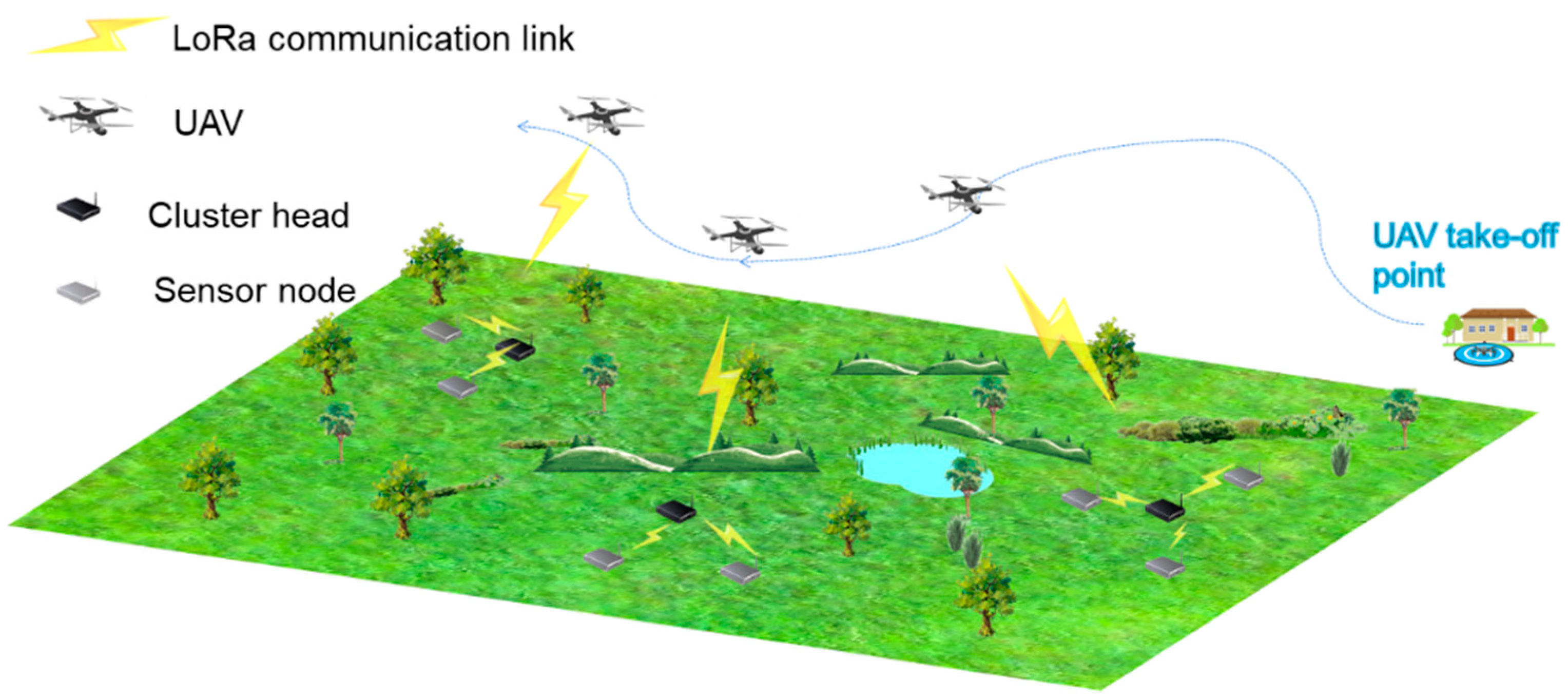
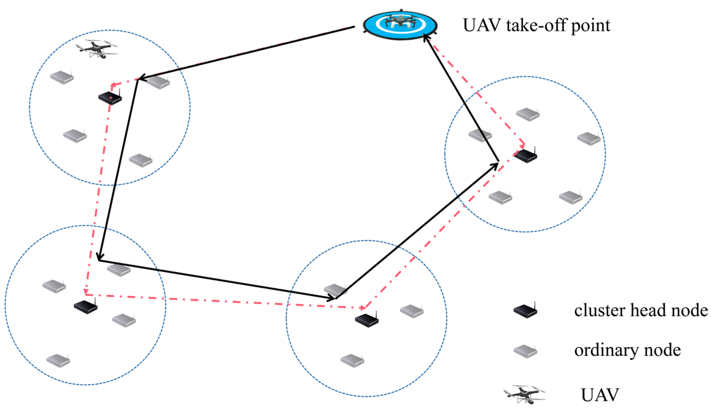
In the paper, we consider the large area environmental monitoring scenarios without infrastructure, using UAV collection data in LoRa networks, as shown in Figure 1. Sensor nodes are deployed in each monitoring area with the clustering structure, in which cluster heads are selected for collecting data of local clusters. Each sensor node is equipped with a solar cell module and various environmental sensors. The UAV collects data from each cluster head using LoRa technology in the whole network, according to the planned path.

Figure 1. Architecture of UAV data collection in the LoRa 2.4 GHz network.

In such systems, how to reduce the UAV flight distance and time is a focus problem, by selecting the proper cluster heads and optimizing the flight route. Moreover, the low data rate of LoRa is a disadvantage for data transmission between UAV and cluster heads, especially for the cluster heads with large amounts of data. At present, many studies based on UAV and LoRa systems mainly use LoRa technology to send control commands to UAVs [7,8,9,10,11], regardless of data rate. However, when cluster heads store a large amount of data, the UAV often needs to hover for data transmission [12]. This will increase the energy consumption of the UAV and reduce the efficiency of the UAV data collection task [13,14].

Motivated by the above challenges, in this paper we propose optimization schemes for UAV data collection with LoRa 2.4 GHz technology in the above scenarios. Firstly, an improved clustering algorithm for the LoRa network is proposed, which considers the influence of distance between the cluster heads and the UAV take-off point. Secondly, we present an improved GA (Genetic Algorithm) for path planning to reduce the UAV flight distance, which introduces the Teaching–Learning-based Optimization (TLBO) [15] and local search optimization algorithms to improve convergence rate and the path solution. Then, an LoRa 2.4 GHz adaptive data rate strategy with a dual channel is designed based on distance and link quality, to reduce the data transmitting time between the UAV and the cluster head nodes, and their energy consumption.

The subsequent sections of this paper are organized as follows. In Section 2 we introduce some related work. Then, Section 3 presents the model formulation and scheme design for UAV data collection in the LoRa 2.4 GHz network. Section 4 tests and analyzes LoRa 2.4 GHz communication performance for UAV and cluster heads. Section 5 presents the simulations and experimental results for the proposed schemes. Finally, Section 6 concludes our work and mentions future work.

2. Related Work

In this section, we introduce the related work of UAV data collection for environmental monitoring in recent years. The properties of our schemes differing from previous work are given at the end of the section.

In some previous studies on data collection using UAV and WSN, the ground nodes were clustered. The researcher introduced a waiting-time-based cluster head with residual energy to ensure the even energy consumption of the head [16]. After the current round of data collection is completed, the next round of cluster head selection is performed. An improved particle swarm optimization algorithm is proposed. Simulation results show that the proposed algorithm is superior to the LEACH algorithm in energy consumption and bit error rate when the UAV travel time is basically the same [17]. The performance gap between them rises with the increase in cluster head nodes. Because of reduced power consumption, the network life can be significantly extended while increasing the amount of data received from the entire network. In [18], the authors proposed a cluster head selection framework assisted by UAV, which collects the residual energy of nodes and uses them to select new cluster heads. The framework can reduce the frequency of cluster head selection of damaged nodes and the number of messages damaged by them. The above clustering methods do not consider the influence of the UAV take-off position on flight distance.

When the cluster heads are selected, UAV path planning needs to be considered to reduce the flight distance. A geometric algorithm based on Hamiltonian is used to determine the optimal flight path of the UAV for agricultural irrigation [16]. In [19], the authors proposed three improved nearest neighbor (NN) algorithms to enhance the performance of data collection by reducing the tour length. The algorithms do not consider the influence of data transmission time. Once the UAV reaches the edge of the sensor node signal coverage, it will fly to the next node. Alemayehu et al. present the efficient FT-DDNN scheme for the shorter flight paths and faster data delivery with fault tolerant capability, in which once the data is collected from the current node, the UAV changes its direction and moves towards the next nearest node instead of going to the center of the current node [20]. Ji et al. proposed an improved dual-population genetic algorithm for UAV flight path planning, which used an additional population to maintain population diversity of the genetic algorithm [21]. Yang et al. designed a penalizing strategy to adjust the fitness of the GA, without the analytical understanding of their geometry structure in the scenarios with no-fly zones [22].

Regarding the communication between UAV and cluster heads, Zigbee is often considered [23,24,25,26]. Nasution et al. designed a telemetry communication system in UAVs using ZigBee protocol [23]. The authors in [27] proposed a UAV-assisted low-consumption time synchronization algorithm for a large-scale WSN. They implemented the algorithm with 30 low-power ZigBee nodes and a UAV on an outdoor highway and an indoor site. Although these studies can be well applied to the UAV application scenarios they describe, as mentioned above, that Zigbee is a short distance communication technology. Therefore, some recent studies have applied LPWAN technologies to UAV communication. LoRa technology is perfect for remote areas without cellular network coverage [28,29,30]. Gallego et al. designed a LoRa UAV gateway to data collection [30]. The results show performance improvements using LoRa-UAV gateways, compared to traditional fixed LoRa deployments, in terms of link availability and covered areas. Kim et al. developed and tested a technology which shared the location of a UAV using LoRa communication and smartphones. The time, location, speed, and direction data from a UAV can be shared to several people through a smartphone application in real time [31]. Saraereh et al. used a relay UAV to transmit messages from a ground-based remote LoRa node to a remote base station, in response to situations where the wireless network may become congested or completely interrupted after a natural disaster occurs [10]. In [11], a communication strategy between a UAV and ground sensor nodes is designed, with 5 GHz and LoRa communication technology. The LoRa module is adopted to wake up the high-power 5 GHz module or put it to sleep, which achieves data collection with a high transmission rate. It reduces the data transmission time and 5 GHz module energy consumption.

Aiming at large data collection of UAV, two heuristic methods are proposed to determine the hovering point of UAV [32]. It also stipulates that the UAV can only collect data from the sensors when it is hovering, and there is no signal transmission when the UAV is moving. On this basis, Gallego et al. improved the above two heuristic algorithms for selecting hovering points of a UAV and stipulated two states of collecting data at hovering points and collecting during flight [33]. Specifically, they defined the sequence of hovering points where the UAV had to hover to gather data and defined a subset of sensor nodes that can send data packets to the moving UAV, to reduce the hovering time and the whole data collection time.

The above works show that the data transmission rate between UAV and ground nodes has an influence on the flight status. When the ground sensor node, using the low data rate LoRa module, stores a large amount of data, the UAV needs to hover to ensure completing data collection. In [11], the UAV adopts a 5 GHz high-speed communication module for the large data collection problem. Thus, the cost and energy consumption of the hardware in the system increases.

Semtech introduced the new long-range 2.4 GHz wireless RF technology and transceiver SX1280 (LoRa 2.4 GHz) in 2017, with the ultra-low current consumption at the higher configurable data rate, compared with the Sub-G LoRa technology. The higher date rate means the lower time on air of the packets, which is conducive to reducing the energy consumption of packet transmission and the probability of channel collision.

In the paper, optimization schemes for UAV data collection with LoRa 2.4 GHz technology are proposed to reduce the UAV flight distance and data collection task time. Some properties of this paper which differ from the previous ones are summarized as follows:

(1)

An improved clustering algorithm for the LoRa network is proposed, which considers the influence of distance between the cluster heads and the UAV take-off point.

(2)

We present an improved Genetic Algorithm to obtain the optimal access path of a UAV, which introduces the Teaching–Learning-based Optimization and local search optimization algorithms to improve convergence rate and the path solution.

(3)

A LoRa 2.4 GHz adaptive data rate strategy with a dual channel is designed based on distance and link quality, to reduce the data transmitting time between the UAV and the cluster head nodes.

(4)

The UAV’s moving status can be adjusted based on data gathering completion status of each cluster head to avoid meaningless flight distances. Real UAV flight paths are obtained to reduce the time of data acquisition tasks.

3. Model Formulation and Scheme Design

3.1. Model Formulation

As shown in Figure 2, energy-constrained sensor nodes are deployed in the monitoring area. The sensor nodes are clustered in a star-shaped topology. The common nodes in the cluster send the collected data to the cluster heads, which fuse the data. The wireless signal coverage of the cluster head nodes is circular. Just above the cluster heads are the possible data collection points. The flying height of the UAV is fixed, and the UAV only needs to communicate with the cluster heads to complete the data collection of the whole cluster. The dashed line is the initial flight path of the UAV, and the solid line is the flight path of the UAV dynamically adjusted according to the LoRa communication strategy. Obviously, it is a TSP problem and belongs to the NP-hard [34] class. We treat the cluster head as a city and the traveling salesman as a drone with sufficient capacity to collect data from all sensor nodes.

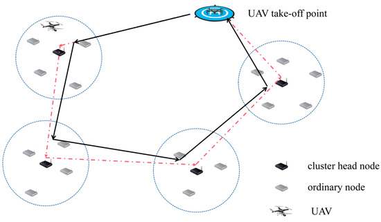
Figure 2. System model formulation.

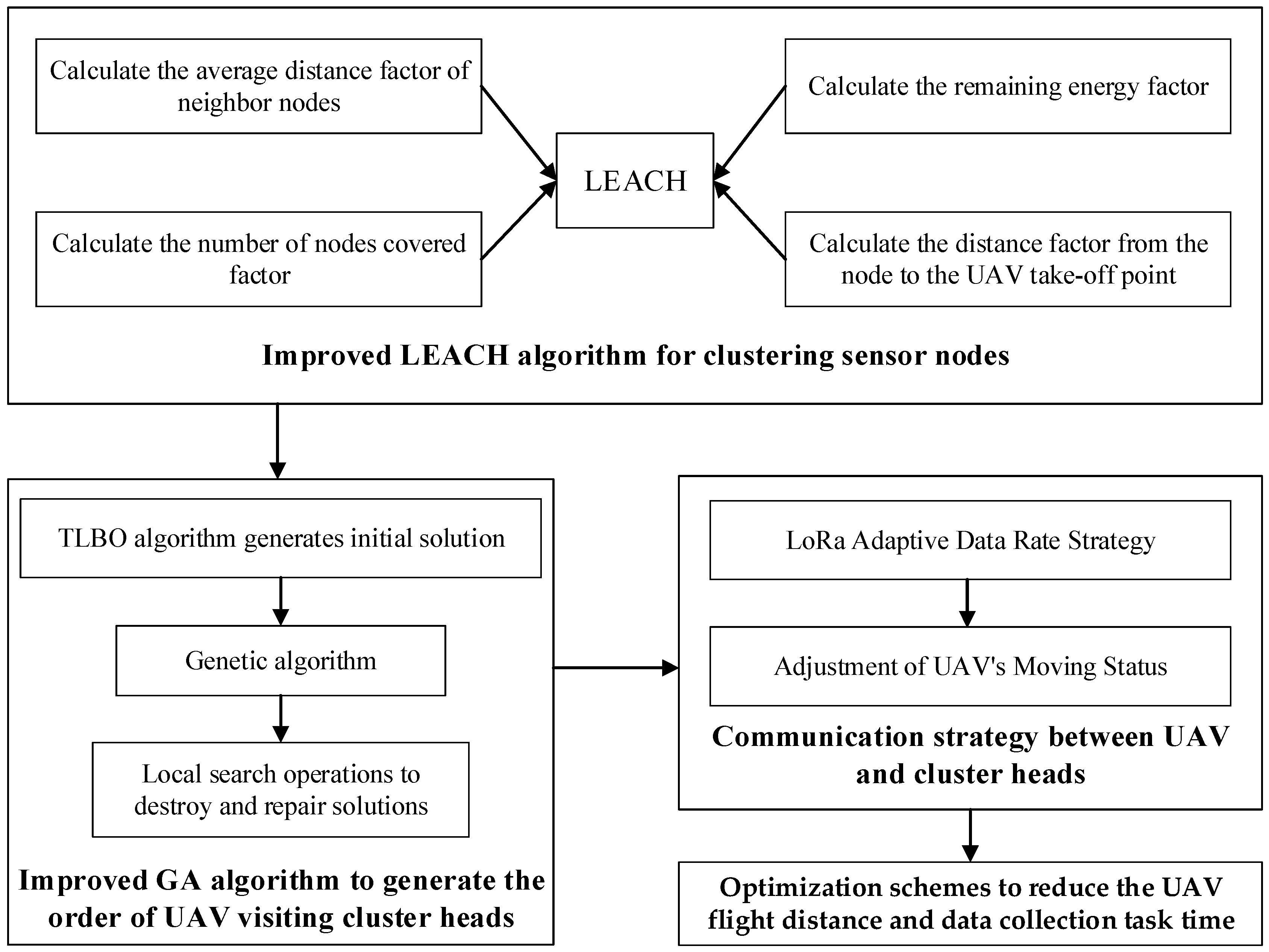
We consider the following three steps to resolve how to reduce the UAV flight distance and data gathering task time. First, an improved LEACH algorithm is designed to cluster sensor nodes. The algorithm considers the location factor of the UAV take-off point, making the cluster head position closer to the UAV take-off point, which is conducive to subsequent path optimization. Then, based on the clustering results, the initial path planning of the UAV is performed with each cluster head node directly above as a possible data collection point. An improved genetic algorithm is designed to optimize it, and an optimal sequence of unmanned access cluster heads is obtained. Finally, according to the LoRa 2.4 GHz adaptive data rate strategy we designed, the communication between the UAV and the cluster head is carried out. The UAV can adjust moving status based on the data gathering completion status of the current cluster head, to reduce the time of the data gathering task. The optimization process is shown in Figure 3. In the paper, we assume that the positions of all sensor nodes are known. The improved LEACH and improved GA algorithms can be executed on the ground computer at the UAV take-off point, in the initial stage. When the planned path is obtained from the ground computer, the UAV starts to carry out the data-gathering task.

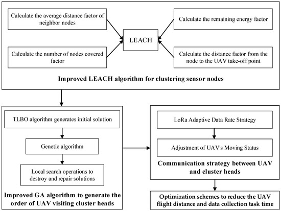
Figure 3. The flow chart of the optimization process.

Descriptions of main notations for the model are explained in Table 1.

Table 1. Descriptions of the main notations.

Notation	Descriptions
DCP	The points directly above each cluster head are data collection points (DCP)
ILEACH	Improved cluster head selection algorithm based on LEACH
TGA	Improved genetic algorithm based on TLBO
DCMDR	Dual Channel Multiple Data Rate
DR	Data Rate
$d{F}_i$	The average distance factor of neighbor nodes
$N{F}_i$	The number of nodes covered factor
$E{F}_i$	The remaining energy factor
$D{F}_i$	The distance factor from the node to the UAV take-off point
L	Path length of UAV traversing cluster head
$x_{ij}$	Binary variable, if UAV goes to cluster head j after arriving at cluster head i, $x_{ij}$ = 1, otherwise is 0
$d_{ij}$	Distance from cluster head i to j
$f(m_j)$	Fitness function
$T_F$	The teaching factor, which determines the degree to which the average value is changed, typically 1 or 2,
$rand$	A random vector, each element of which is a random number in the range of [0, 1].
$R(i,j)$	The correlation formula between cluster head i and j
$\sigma$	Current solution
${\sigma }^{\prime }$	Updated solution
$v$	The UAV’s flight speed
$m$	The data rate obtained from ACK
$b$	The data size stored by the cluster head

3.2. Improved Clustering Algorithm

The clustering algorithms divide the nodes of a sensor network into different clusters, each cluster has only one cluster head node. Regarding the UAV data collection scenario in the paper, the cluster head gathers the data of sensor nodes in the cluster, and then sends the data saved to UAV when it arrives. The closer the cluster heads are to the UAV take-off point, the shorter the flight distance of UAV will be. The typical clustering algorithms are LEACH (Low Energy Adaptive Clustering Hierarchy) [35], TEEN (Threshold sensitive Energy Efficient sensor Network protocol) [36], PEGASIS (Power-Efficient Gathering in Sensor Information System) [37], etc. The TEEN algorithm uses the filtering method to reduce the amount of data transmission; however, the threshold setting prevents some data from being reported. The PEGASIS algorithm adopts a chain method, and node damage may lead to the failure of the chain. The above two algorithms are not suitable for the application scenario of the paper. In the process of selecting the cluster head in the LEACH algorithm, the nodes in the network act as the cluster head with equal probability. Specifically, each node randomly selects a value between [0, 1]. If the selected value is less than a certain threshold, the node becomes the cluster head. Due to the randomness of cluster head selection and the fact that the residual energy of nodes is not considered, the rationality of the number of cluster heads and the uniformity of distribution in the network cannot be guaranteed. Therefore, we propose an improved cluster head selection algorithm based on LEACH (ILEACH), which is aware of the distance from the cluster heads to the UAV take-off point, while considering the factors of remaining energy, number of nodes covered, and average distance of neighbor nodes.

The average distance factor of neighbor nodes is represented by $d{F}_i$, which is expressed by $d{F}_i=\frac{1}{d(i)}$, where $d(i)$ is the average distance from all neighbor nodes of i within the radius $R_c$ to $i$. The smaller $d(i)$ is, the shorter the average distance between the surrounding nodes and node i is. Then, when the surrounding nodes communicate with this node, the average energy consumption is smaller.

$N{F}_i$ represents the number of nodes covered factor, which is expressed by $N{F}_i=1-\frac{1}{Nu(i)}$, where $Nu(i)$ is the number of nodes contained in node i within the range of $R_c$. The larger the $Nu(i)$, the better coverage performance of the cluster headed by this node.

$E{F}_i$ represents the remaining energy factor, which is expressed by $E{F}_i=e^{\frac{E_R}{E_I}}$, where $E_R$ is the remaining energy, and $E_I$ is the initial energy of the battery.

$D{F}_i$ represents the distance factor from the node to the UAV take-off point, which is expressed by $D{F}_i=\frac{1}{D(i)}$, where $D(i)$ is the distance from node i to the UAV take-off point.

The specific steps of the improved algorithm are as follows:

Each node calculates its own delay time $t_c(i)$ by (1). If node i does not receive information from the cluster head within time $t_c(i)$, it announces that it is the cluster head and broadcasts notifications to its neighbors.

If the node receives the cluster head information, the node is selected as a member node and the timing is exited.

The node chooses to join the cluster that has received the cluster head information late, if it receives more than one cluster head information.

$$t_c(i)=\alpha \times e^{-{\theta }_i}$$

(1)

$${\theta }_i=100\times \left[{\omega }_1\cdot d{F}_i+{\omega }_2\cdot N{F}_i+{\omega }_3\cdot E{F}_i+{\omega }_4\cdot D{F}_i\right]$$

(2)

$$d(i)=\frac{{\displaystyle \sum _{j-Ne(i)}d(i,j)}}{Nu(i)}$$

(3)

In the above formulas, $\alpha$ is the proportional coefficient that determines the delay size; $d(i,j)$ denotes the distance between any two nodes i and j. When $d(i,j)\le R_c$, node j is called the neighbor node of i. $R_c$ is the effective broadcast radius of node i, the set of neighbor nodes of node i is represented by $Ne(i)$; ${\omega }_1$, ${\omega }_2$, ${\omega }_3$, ${\omega }_4$ is the weight assigned to each metric, respectively, and ${\omega }_1+{\omega }_2+{\omega }_3+{\omega }_4=1$.

3.3. Path Optimization

3.3.1. Path Optimization Model

This section aims to find the shortest planned flight path of a UAV. To simplify the model, we assume that the points directly above each cluster head are data collection points (DCP). The UAV starts from the take-off point, and then traverses all DCPs at a fixed speed and height, and finally returns to the take-off point.

The optimization of the UAV path is to minimize the flight distance $L$, expressed as follows:

$$L=\min \sum _{i\ne j}^{}{x}_{ij}{d}_{ij}$$

(4)

$$s.t=\{\begin{array}{l}{\displaystyle \sum _{j=1}^{n+1}{x}_{ij}=1,\hspace{1em}i=1,2,\dots ,n+1}\\ {\displaystyle \sum _{i=1}^{n+1}{x}_{ij}=1,\hspace{1em}j=1,2,\dots ,n+1}\\ {\displaystyle \sum _{i=1}^{n+1}{\displaystyle \sum _{j=1}^{n+1}{x}_{ij}=n+1,\hspace{0.17em}i,j\in O}}\\ x_{ij}\in \{0,1\},\hspace{1em}i,j\in O\end{array}$$

(5)

where i and j are the number of DCPs, $i,j\in O$, $O=\{1,2,\dots ,n+1\}$, $n$ is the total number of DCPs, $i=1$ represents the UAV take-off point; $d_{ij}$ represents the distance from i to j; $x_{ij}$ is the decision variable, representing the UAV from i to j. If i is not equal to j, $x_{ij}$ takes 1, otherwise 0. Equation (5) represents the constraint condition, the objective function must meet the requirement that any DCP is traversed and only traversed once, any possible traversal sequence must include all DCPs.

As a TSP problem, which needs to be addressed by heuristic algorithms, such as particle swarm optimization algorithm [38], ant colony optimization [39], artificial bee colony algorithm [40], fruit fly optimization algorithm [41], tabu search algorithm [42], and simulated annealing algorithm [43], the genetic algorithm (GA) has shown good performance in solving problems such as task assignment and route optimization. The advantages of the GA in real applications have also been demonstrated [21,22].

3.3.2. Description of the TGA Algorithm

The genetic algorithm (GA) is a heuristic search algorithm based on the process of biological evolution, which generates the next generation of solutions through selection, crossover, and mutation. In this process, the solution with a low fitness function value is gradually eliminated, and the solution with a high fitness function value is increased, so as to approach the optimal solution of the problem gradually through evolution. The algorithm has the advantages of being simple and general, strong robustness, and suitable for parallel processing. However, the local search ability of the genetic algorithm is poor, and the initial solution is uncertain. At this stage, the algorithm is used for blind search and makes the convergence rate slower. Similar to the GA algorithm, the Teaching–Learning-Based Optimization algorithm (TLBO) is also a population-based heuristic stochastic optimization algorithm, which is inspired by the classroom teaching process and imitates the teacher’s influence on students. On the one hand, the number of hyperparameters in TLBO is lower; thus, the search speed is fast. On the other hand, the optimal solution obtained is not as good as the GA. Furthermore, novel state transition rules are utilized to avoid the local optimal and improve the quality of solution. The TGA (improved genetic algorithm based on TLBO) algorithm designed combines the advantages of the two algorithms, which considers the convergence rate while obtaining a better solution.

First, the UAV path planning model is solved by TLBO with fast convergence, and the sub-optimal solution is used as the initial solution of the GA. In the TLBO algorithm, the higher the individual’s learning performance, the better the individual. The goal of UAV flight path optimization is to obtain the shortest flight distance, so the fitness function of TLBO is Equation (6), where M is the number of students.

$$f(m)=\frac{1}{L_m}\hspace{1em}m\in \{1,2,\dots ,M\}$$

(6)

In the teaching phase, students improve their own level by learning the difference between the teacher and the average level of the class. For the jth learner $m_j$ in the group, the update mechanism is expressed as follows:

$$m_j^{\prime }=m_j+rand\cdot (m_t-T_F\cdot m_{mean})$$

(7)

$$m_{mean}=\frac{{\displaystyle {\sum }_{j=1}^M{m}_j}}{M}$$

(8)

$$T_F=round\left[1+rand(0,1)\right]$$

(9)

where $m_j^{\prime }$ is the known solution $m_j$; $m_t$ is the current optimal UAV flight path; $m_{mean}$ is the average state of the population; $T_F$ is a teaching factor, which determines the degree to which the average value is changed, typically 1 or 2, which is an important step in the heuristic; $rand$ is a random vector, each element of which is a random number in the range of [0, 1].

In the learning phase, learning occurs by simulating the way students communicate with each other in order to improve their own level. For $m_j$, the updated formula is:

$$m_j^{\prime }=\{\begin{array}{l}{m}_j+rand\cdot (m_k-m_j),\hspace{0.17em}if\hspace{0.17em}f(m_j)<f(m_k)\\ m_j+rand\cdot (m_j-m_k),\hspace{0.17em}otherwise\end{array}$$

(10)

where $m_j^{\prime }$ is the new value of flight path $m_j$, $m_k$ is another randomly chosen flight path from the population that is different from $m_j$. $f(m_j)$ and $f(m_k)$ are the fitness of paths $m_j$ and $m_k$, respectively. $rand$ is a random vector, each element of which is a random number in the range of [0, 1]. Similar to the teaching phase, the value of $m_j$ will adopt the larger one between its original fitness and the new fitness, and then enter the next round of teaching. The generated suboptimal solution is used as the initial solution of the TGA algorithm, when the TLBO reaches the set number of iterations and terminates.

A local search update mechanism is added to enhance the local search capability of the TGA algorithm. In order to avoid premature convergence of the algorithm during the calculation process, the result of the non-global optimal solution appears.

The solution generated by each iteration is broken and then repaired. Specifically, firstly a DCP is randomly removed from the current solution $\sigma$ to set $S$, as the first element of set $S$, $p$ represents the number of stay points removed, and there are still $p-1$ elements left. Then, a DCP $z$ is randomly selected from the set $S$ each time, and the remaining DCPs $z$ in $\sigma$ are arranged in ascending order of correlation. The DCP$c$ is selected from $\sigma$ that has the greatest correlation with $z$, $c$ is removed from $\sigma$, and added to $S$. This process is repeated $p-1$ times until the remaining $p-1$ elements are selected. $c_{ij}$ is the Euclidean distance between $i$ and $j$. The correlation formula is:

$$R(i,j)=\frac{\max c_{ij}}{c_{ij}}$$

(11)

In actual situations, there is no perfect correlation function. If over-reliance on the correlation function selects the DCP to be moved, it may be limited to local correlation. To avoid this situation, a random element $\gamma$ needs to be added to the algorithm. ${\sigma }^{,}$ is the number of DCPs remaining in $\sigma$.

$$\gamma ={(Random([0,1]))}^D\times \hspace{0.17em}{\sigma }^{,}$$

(12)

The remaining DCPs in $\sigma$ are arranged in descending order of correlation with $z$, and the sorted sequence is $l_{st}$, so the result of the above process is $l_{st}[index]$. $D$ is a random number not less than 1. From that we can conclude, when $D$ is 1, the DCP that is removed is completely selected at random; when $D$ is equal to positive infinity, it is close to selecting the DCP with the greatest correlation. In other words, the higher the value of $D$ is, the more favorable it is to the DCP with high correlation.

Finally, the damaged solution is repaired, and the elements in the removed DCPs set $S$ are reinserted back into the partial solution ${\sigma }^{\prime }$ to produce a better solution. First, the optimal insertion position of each DCP in $S$ is calculated, and the DCP $c$ in $S$ is inserted back into the partial solution ${\sigma }^{\prime }$. In the process of selecting the DCP $c$ from $S$ and inserting it back to ${\sigma }^{\prime }$, the increment of the objective function value is calculated where each DCP in $S$ is inserted into its optimal insertion position, and the DCP with the largest increment is chosen as the first insertion point. The method is repeated until all the DCPs are reinserted into the partial solution.

The steps of the TGA algorithm are described as shown in Algorithm 1.

Algorithm 1 Implementation of the TGA algorithm

Input: Maximum number of iterations, all cluster head nodes $(x_i,y_j)$, UAV take-off point $(x_0,y_0)$, population size, crossover probability $P_c$, probability of variation $P_m$ Output: The optimal transportation route. Perform TLBO algorithm to randomly initialize population Evaluate population$m_{mean}$ While (number of iterations)   for all port do     TLBO algorithm produce $m_j^{\prime }$   end for end while Execute the GA algorithm, using solution $m_j$ generated by TLBO as the initial solution of the improved GA algorithm While (number of iterations)   for each individual do     Calculate the objective function for each individual based on (4)     Crossing and mutation to produce a new generation of population     New-generation populations perform local search operations with the concept of destruction and repair     Delete duplicate individuals from the population and complete the deleted individuals   end for Update parameter $R(i,j)$, $\gamma$ according to Equations (11) and (12) end while

3.4. Communication Strategy

3.4.1. LoRa Adaptive Data Rate Strategy

To reduce the data transmitting time between the UAV and the cluster head nodes, a LoRa 2.4 GHz adaptive data rate strategy with a dual channel is designed. The UAV is equipped with two LoRa 2.4 GHz transceivers—SX1280, and the ground cluster head node with one. On the UAV, one SX1280 is used for Channel 1 to establish a connection and transmit a command between the UAV and the cluster head node, the other is used for Channel 2 to transmit sensor data.

SX1280 can be configured to different Data Rates (DR) as shown in Table 2 Each DR value corresponds to a specific combination of Modulation mode, Spreadind Factor (SF), and Bandwidth (BW). In LoRa mode, a lower DR can have a longer transmission distance, and increase the success rate, as the receiver sensitivity will be better. The FLRC modulation with 1040 Kbit/s rate is also supported for applications requiring higher data rates and operating over substantially shorter ranges.

Table 2. Spread spectrum factor and data rates.

Data Rate (DR)	DR6	DR5	DR4	DR3	DR2	DR1	DR0
Bandwidth (kHz)	1200	300	812	812	812	406	203
Mode	FLRC	FLRC	SF7	SF9	SF11	SF12	SF12
Physical Bit Rate (kb/s)	1040	260	44.41	14.27	4.36	1.19	0.595
Receiver Sensitivity (dBm)	−100	−106	−112	−117	−123	−128	−130

In our system, the DCMDR (Dual Channel Multiple Data Rate) scheme is presented, as shown in Figure 4. The Channel 1 constantly uses DR0 with the farthest communication distance, and the Channel 2 uses the variable DR according to the wireless condition. The ground cluster head nodes use the (low power listening) LPL-like method to check the Channel 1 using DR0, to reduce the energy consumption. In the course of the flight, the UAV continually sends wake-up packets by DR0 in Channel 1 with the target cluster head node ID. When the ground cluster head node is awakened and receives the wake-up packet, if the node ID is not equal to its own, it returns to LPL status. Otherwise, it replies with an ACK packet with the RSSI, SNR, and the data size information to the UAV. The UAV chooses the proper DR for data transmitting, according to the distance to the cluster head node and the ACK packet information piggybacked. When it negotiates the DR for data transmitting with the cluster head node, it switches to the new DR in Channel 2 for data receiving. The cluster head also switches to the same DR and starts to transmit the data packet to the UAV. When the UAV receives one data packet, it returns a data ACK packet. If the cluster head node does not receive the ACK within the preset timeout period and times, it switches to DR0, and negotiates the new and slower DR for data transmitting with UAV. The above process is repeated until the data packet is successfully transmitted.

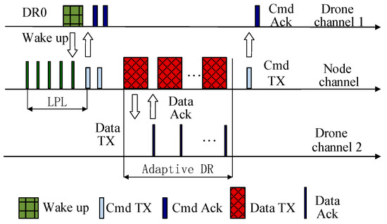
Figure 4. DCMDR scheme.

The moving status of the UAV is determined based on the completion of receiving data. Thus, the UAV adaptively adjusts $DR\in \{6,5,\dots ,0\}$ according to the distance, RSSI, and SNR to reduce data transmission time, the DR should be as high as possible, while ensuring the packet loss ratio. According to (13), the threshold condition of DR6 is determined first, then the condition of DR5 is determined, and so on.

$$DR=\{\begin{array}{l}6\hspace{1em}if\hspace{0.17em}SN{R}_{th6}<\overline{SNR}\hspace{0.17em}and\hspace{0.17em}RSS{I}_{th6}<\overline{RSSI}\hspace{0.17em}and\hspace{0.17em}Dis{t}_{th6}<\overline{Dist}\\ 5\hspace{1em}else\hspace{0.17em}if\hspace{0.17em}SN{R}_{th5}<\overline{SNR}\hspace{0.17em}and\hspace{0.17em}RSS{I}_{th5}<\overline{RSSI}\hspace{0.17em}and\hspace{0.17em}Dis{t}_{th5}<\overline{Dist}\\ n\hspace{1em}else\hspace{0.17em}if\hspace{0.17em}SN{R}_{thn}<\overline{SNR}\hspace{0.17em}and\hspace{0.17em}RSS{I}_{thn}<\overline{RSSI}\hspace{0.17em}and\hspace{0.17em}Dis{t}_{thn}<\overline{Dist}\\ 0\hspace{1em}else\end{array}$$

(13)

$SN{R}_{thn}$, $RSS{I}_{thn}$, $Dis{t}_{thn}$ are the thresholds of SNR, RSSI, and distance for selecting $D_{rn}$, where $SN{R}_{thn}<\overline{SNR}$, $RSS{I}_{thn}<\overline{RSSI}$, $Dis{t}_{thn}<\overline{Dist}$. It means when $SNR$, $RSSI$, and $Dist$ all exceed the threshold values of a DR, the DR can be selected.

The thresholds are different in different scenarios and conditions and can be obtained by experiments in application scenarios.

3.4.2. Adjustment of the UAV’s Moving Status

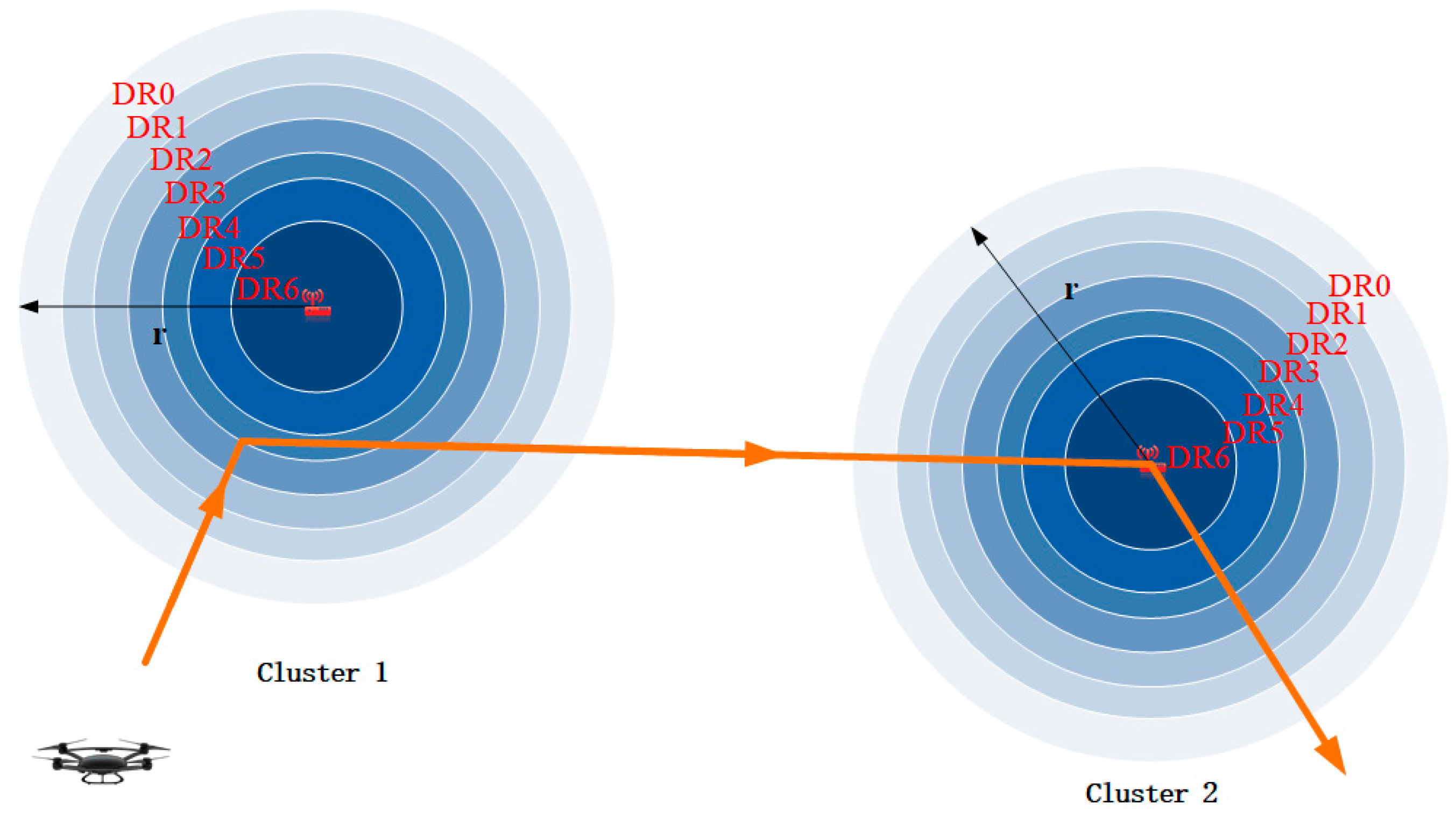
After the planned path is obtained by the TGA algorithm, the UAV flies to each cluster in the order of the planned path. As shown in Figure 5, the area covered by the signal of the cluster head is a circle with a radius of $r$ and the center at the position of the cluster head. The UAV begins to fly at a constant speed and altitude.

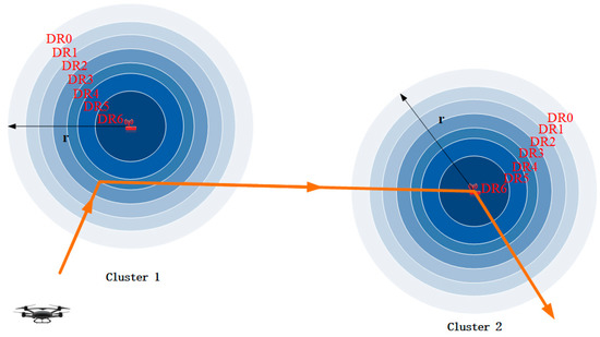
Figure 5. Adjustment of the planned flight path.

According to DCMDR, the communication range of the cluster head is divided into different regions with different DRs. With the region closer to the cluster head, the DR assigned is higher.

The longest distance the UAV can fly within the signal coverage of the cluster head is $2r$ m. The UAV’s flight speed is $v$ m/s, the data rate obtained is $m$ bit/s. Therefore, when the UAV flight speed is constant, the theoretical maximum amount $b_1$ of data received by the UAV within the signal range of cluster head is as follows:

$$b_1=2{\displaystyle \sum _{DR=0}^6{m}_{DR}\cdot \frac{r_{DR}-r_{DR+1}}{v}}$$

(14)

According to (14), it can be seen that $b_1$ is affected by $m_{DR}$ and $v$. When the data rate is certain, the faster the UAV’s speed is, the smaller $b_1$ will be. Thus, we assume the data size stored by the cluster head is $b$ bits: there will be two cases. The first case is $b\le b_1$, when the UAV crosses the signal coverage area of the cluster head, data collection can be completed without adjusting the speed. In addition, in order to reduce unnecessary flight distance, after receiving the data of the current cluster head, the UAV will fly to the next cluster head according to the visit sequence of the planned path, as shown in cluster 1 in Figure 5. The second case is when $b>b_1$, that is, the UAV is moving at the current speed and cannot collect the data completely within the signal coverage of the cluster head. In order to complete data gathering efficiently, the UAV needs to reduce the speed within the signal coverage of DR6, as shown in cluster 2 in Figure 5. On the basis of obtaining the planned path through the TGA algorithm, using DCMDR and Adjustment of UAV’s Moving Status, we call it the TGA-MOVING-DCMDR method.

4. Field Test

The thresholds of DR are different in different scenarios and conditions, and we can obtain them by testing in application scenarios. To obtain the thresholds we conducted a lot of field tests and tested the RSSI and packet loss ratio at different distances. To prove the effectiveness and reliability of LoRa 2.4 GHz and DCMDR, we tested the data transmitting time for one cluster head.

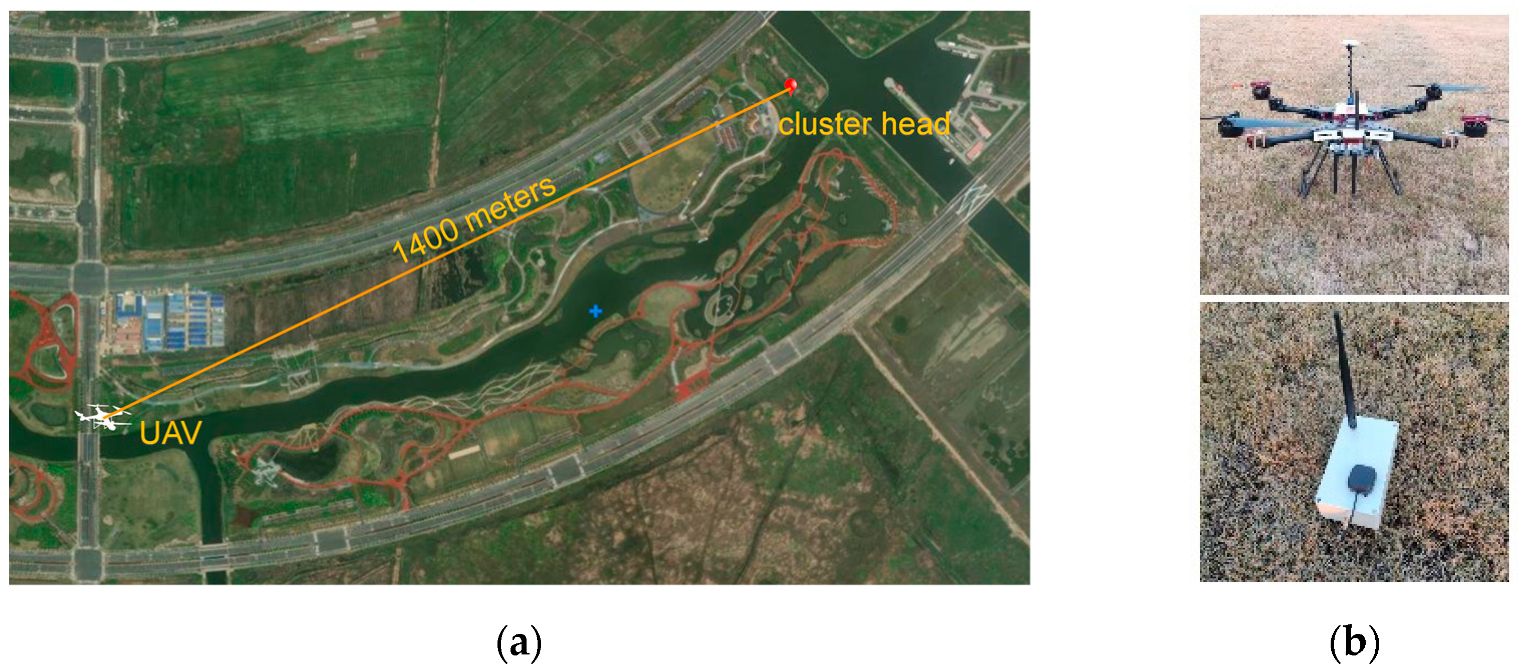
All tests were conducted in Lingang area of Shanghai, as shown in Figure 6a. In the test scenario, there is a slight occlusion between the ground and the air. Figure 6b shows an aerial UAV platform with a dual-channel LoRa module and a cluster head node. The LoRa module uses SX1280, a rubber duck omnidirectional antenna, 2.4 GHz band, and 3 dBi gain. All tests were carried out within a fixed transmission power of 12.5 dBm, CR = 4/5, and pre-tone length = 8 symbols, and the transmission mode DR ranges from 0 to 6. The flying height of the UAV is 30 m, the low flight speed of 4 m/s is used to obtain the thresholds.

Figure 6. Real-world test. (a). Experimental site. (b). Sensor node and UAV air platform.

4.1. Threshold Test

The test evaluated the influence of distance on RSSI and packet loss ratio by different DRs, and 100 packets were sent by the cluster head at a time, the size of the packet is 100 bytes. The cluster head node was placed at the target position of the UAV and then the UAV moved to the cluster head along its initial heading over a straight distance of 1400 m in steps of 50 m measured by GPS. At each step, the receiver of the UAV acquired the RSSI sample mean and packet loss ratio by 7 different DRs, respectively; the routine was repeated 20 times.

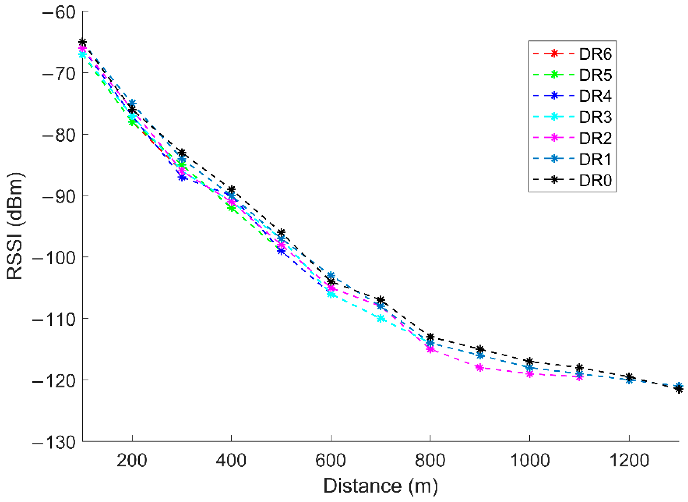
Figure 7 presents the average results of RSSI attained from the test. It is obvious that the RSSI results by all DR modes quickly decreased with increase in the distance, when the distance was less than 800 m. When the distance exceeded 800 m, with increase in the distance, the RSSI value decreased correspondingly, and the downward trend became gradually slower. It is worth noting that with the increase in DR, when the distance exceeded a certain value, the UAV can hardly receive data packets.

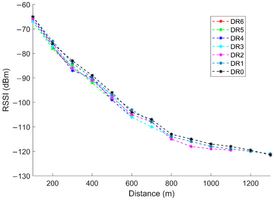
Figure 7. Evaluation of the RSSI.

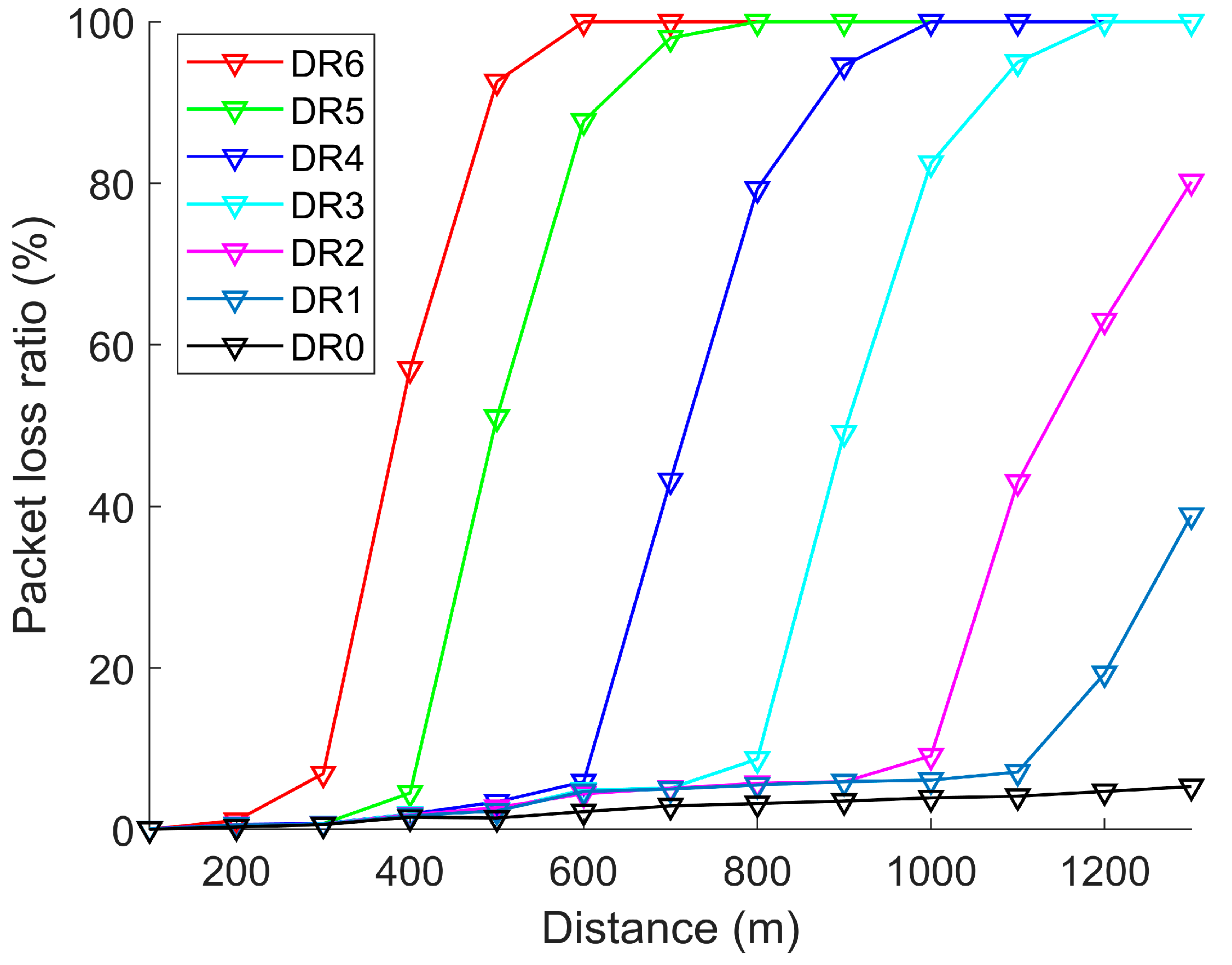
Figure 8 shows the average packet loss ratio with different distances. It can be seen that the packet loss ratio of all DRs increases as the distance increases. When the distance was 300 m, the packet loss rate of DR6 was 6.9%, and then the packet loss ratio increased rapidly as the distance increased. When the distance was 500 m, the packet loss ratio of DR6 reached 100%. DR5, DR4, and DR3 also have a similar trend. When the distance exceeded 400, 600, and 800 m, the packet loss ratio of DR5, DR4, and DR3 increased rapidly as the distance increased. When the distance was 1000 m, the packet loss ratio of DR2 was 8.8%, and the packet loss ratio of DR1 was 5.0%. Subsequently, the packet loss ratio of DR2 increased rapidly until the distance was 1100 m, which had reached 43.3%. When the distance was 1100 m, the packet loss ratio of DR1 was 5.0%, and then it increased rapidly as the distance increased, and the changing trend was slower than that of DR2. Moreover, the packet loss ratio of DR0 was always less than 5% when the distance was within 1300 m.

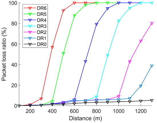
Figure 8. Evaluation of the packet loss ratio.

Figure 7 and Figure 8 both show that different DRs are only meaningful within the certain distance range. We selected the distance when the packet loss rate is 5% as the DR distance threshold $Dist$ in (13). Through the above tests, the threshold values of SNR, RSSI, and $Dist$ of each DR in this environment can be obtained, as shown in Table 3.

Table 3. The thresholds of SNR, RSSI, and Dist for each DR.

DR	SNR	RSSI	Dist (m)
6	0	−85	250
5	0	−95	380
4	0	−112	600
3	−5	−114	750
2	−10	−119	950
1	−15	−120	1100

4.2. Data Gathering Time Test

The test evaluates the influence of data size on data gathering time. The cluster head node was placed at the target position of the UAV and then the UAV moved to the cluster head along its initial heading over a straight distance of 1300 m. According to Table 3, we defined the time when the UAV enters an area 1300 m away from the cluster head as the beginning of the data gathering task, and the data gathering time is from the beginning of the data gathering task to the completion of the data transmission. We tested the data gathering time using DCMDR, DR0, DR3, and DR6 data rate modes, with the stored data of cluster head from 0.1 to 100 Mbits, respectively. The results are shown in Figure 9. The data gathering time of DCMDR is always the smallest regardless of the data size. The data gathering time of DR0 and DR3 modes increases rapidly as the amount of data increases. When the data size of DR0 exceeds 1 Mbits, and the data size of DR3 exceeds 25 Mbits, their data gathering time exceeded 2000 s. The reason is that the data rate of DR0 and DR3 is lower, when the amount of data is large, the UAV cannot guarantee that the data is gathered within their $Dist$. It needs to reduce flight speed to ensure complete data gathering according to (14), and the data gathering task cannot be completed due to the limited flight time. Although the DR6 has the fastest data rate, when the data size is less than 1 Mbits, the data gathering time is much longer than DCMDR. It is because the $Dist$ of DR6 is the smallest, and the UAV has to fly into the coverage area of DR6 for a long time, while the DCMDR can start gathering data from a long distance with the lower DRs. Therefore, DCMDR has good adaptability to the size change of data gathered.

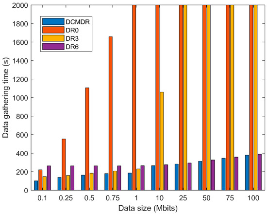
Figure 9. Data gathering time varying with data size.

5. Simulation and Experiment

In Section 5.1, we built our schemes into a custom Matlab simulator based on an SX1280 transceiver, to evaluate the performance of ILEACH, TGA, and DCMDR. In Section 5.2, the experiments were carried out to verify the effectiveness of the schemes.

5.1. Simulation

Firstly, we used the standard data set (Solomon benchmark datasets R201, C201, and RC201) [44], which includes the coordinates of nodes, to simulate the TGA algorithm, and verify the solution quality of TGA in path optimization.

Secondly, to verify the advantages of combining algorithms (ILEACH-TGA and TGA-MOVING-DCMDR), in our simulations, 200 sensor nodes were distributed uniformly at random in an area of 10,000 m, with the UAV’s take-off point (5000, 5000). The data gathering model corresponds to the context of the aforementioned real-world field tests.

5.1.1. Simulation and Analysis of ILEACH and TGA Algorithms

In this section, we verify the advantages of the ILEACH algorithm and TGA algorithm in generating a UAV flight path. Without loss of generality, we took the coordinate data contents of three classical datasets (Solomon benchmark datasets R201, C201, and RC201), 100 nodes in each dataset, to test the performance of the TGA algorithm for the route optimization problem. Among them, the node locations of C201 data are relatively concentrated, while those of R201 data are relatively scattered, and those of RC201 data are uniform. The basic GA algorithm and TGA algorithm were, respectively, run 30 times. Their results are shown in Table 4. The results show that the optimal solution and average solution obtained by the TGA algorithm are better than the GA algorithm. Among them, in the three data sets, the optimal solution of the TGA algorithm is 64.83%, 65.30%, and 73.67% less than the GA algorithm respectively, and the average solution is 71.71%, 71.88%, and 74.36% less than the GA algorithm, respectively. It is because the addition of the local search update mechanism improves the quality of the solution. In terms of convergence rate, the average convergence algebra of the TGA algorithm is less than that of the GA algorithm, and the convergence effect of the GA algorithm is not obvious within 200 generations. This may be because the genetic algorithm is sensitive to the initial solution, and the initial solution of TGA is generated by the TLBO algorithm, which is more accurate than the initial solution randomly generated by the traditional GA algorithm.

Table 4. Results obtained using GA and TGA.

Datasets	TGA			GA
	Optimal Solution (m)	Average Solution (m)	Average Convergence Algebra	Optimal Solution (m)	Average Solution (m)	Average Convergence Algebra
R201	707.5	712.1	60	2011.6	2517.3	164.7
C201	723.3	735.4	79.3	2084.5	2615.5	159.7
RC201	696.5	701.6	87.5	2646.2	2737.2	194.3

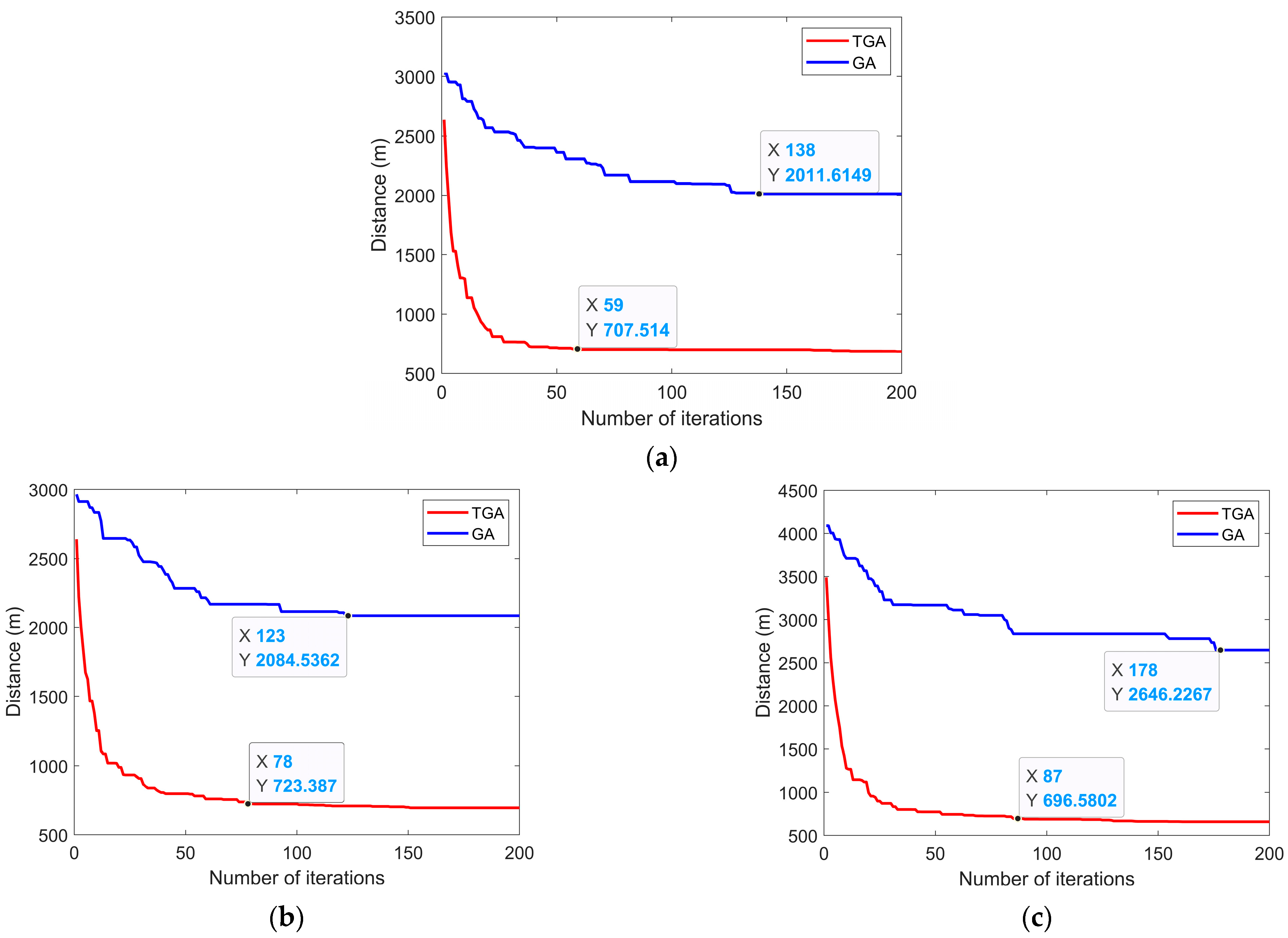
Figure 10 shows the convergence process of the basic genetic algorithm and TGA algorithm to solve the data sets R201, C201, and RC201. As the number of iterations increases, the total distance of the two algorithms decreases. The TGA algorithm obviously converges within 200 generations, while the GA algorithm has a slow convergence rate, almost no convergence, and the optimization effect is quite different from the TGA algorithm. The simulation results show that the TGA algorithm has obvious advantages in optimization result and convergence rate, regardless of the density of node distribution.

Figure 10. Convergence comparison for (a) R201); (b) C201; and (c) RC201.

To verify the advantages of combining ILEACH and TGA algorithms (ILEACH-TGA), we uniformly randomly distributed 200 wireless sensor nodes in an area of 10 km × 10 km and used a UAV for data collection. The coordinate of the UAV’s take-off point was (5000, 5000). The LEACH and ILEACH algorithms were used for clustering, and UAV path planning was performed with the GA and TGA algorithms, according to the clustering results, respectively. The averaged results of 30 runs are shown in Figure 11.

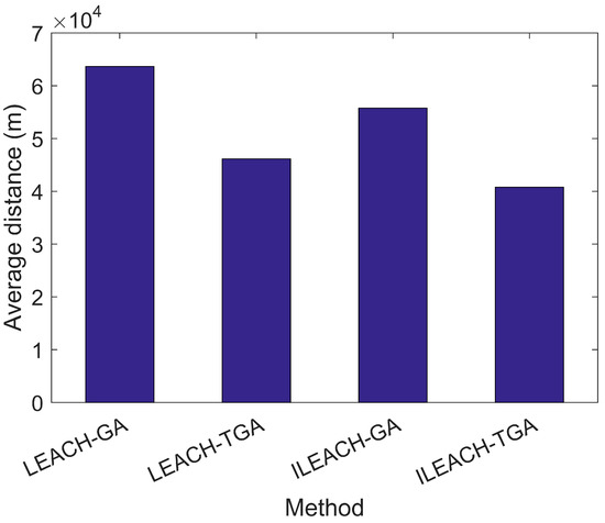
Figure 11. Average path length comparison.

It can be seen that the average distance of the planned path by ILEACH-TGA is significantly smaller than the other methods. The average path length of LEACH-GA is the largest, which is slightly larger than that of ILEACH-GA. In the case of using the same path optimization algorithm and only changing the clustering algorithm, the results of ILEACH are better than LEACH. It is because the distance factor from the node to the UAV take-off point is added to the ILEACH algorithm. The result shows that, in the combination of clustering algorithm and path optimization algorithm, the combination of ILEACH and TGA has the best optimization effect.

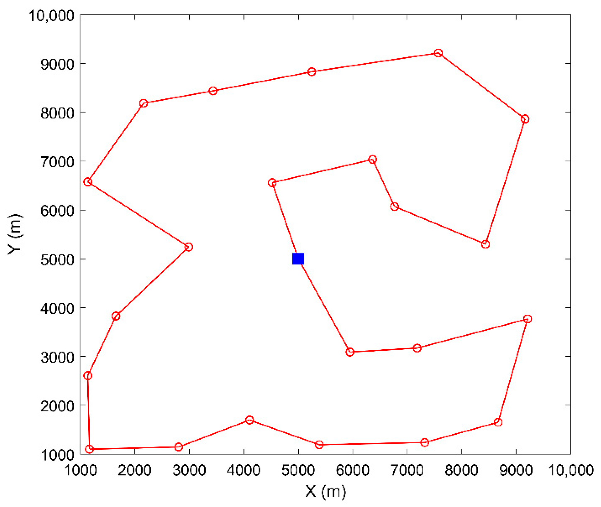
Figure 12 and Figure 13 are the shortest paths obtained by ILEACH-GA and ILEACH-TGA from the 30 runs, in which red dots represent cluster heads and blue squares represent take-off points.

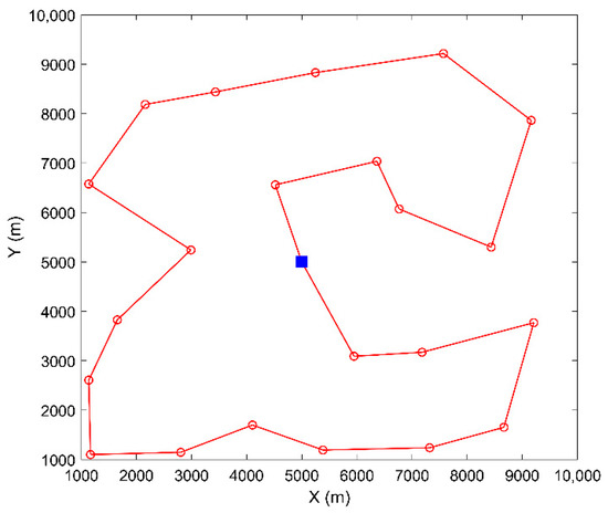
Figure 12. TGA’s UAV planned path.

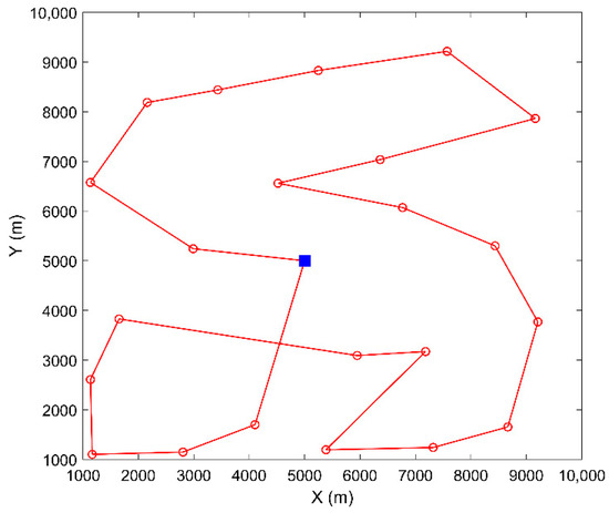
Figure 13. GA’s UAV planned path.

5.1.2. Simulation and Analysis of TGA-MOVING-DCMDR

In this section, the DCMDR is used to reduce the data gathering time between the UAV and the cluster heads. The influences of data size in cluster heads, UAV flight speed, and the number of sensor nodes on the completion time of the data gathering task are evaluated.

As analyzed above, the ILEACH algorithm has advantages in clustering, and is used in simulations. The GA and TGA algorithms are used to obtain the planned path. We call the mode, in which the UAV can only collect data when hovering over the cluster head [32], as the HOVER collection. The mode in [20] is called the MOVE collection, in which the UAV flies to the current cluster head and collects data at the same time. When the amount of data is large, it needs to hover over the current cluster head to complete the data gathering. After completing data gathering, it flies directly to the next node using fixed flying speed. In our schemes, the MOVING collection mode is defined, in which the flying speed of the UAV can be adjusted to complete the data gathering task. Moreover, as shown in Figure 7, at a fixed data rate, the data gathering time of DR6 is always minimal, regardless of data size. Therefore, we use DR6 for all HOVER and MOVE modes. We compare our joint method TGA-MOVING-DCMDR with GA-HOVER-DR6, TGA-HOVER-DR6, GA-MOVING-DCMDR, and TGA-MOVE-DR6 to evaluate the performance.

In scenario 1, we evaluated the influence of the average amount of data in cluster heads on the completion time of data gathering task. The flight speed of the UAV was set to 12 m/s. We evaluated the large amount and small amount of data in cluster heads, respectively. The simulations were implemented with 20 consecutive runs, and the average results are shown in Figure 14. It is obvious that the completion time of the TGA-MOVING-DCMDR method is always the minimum, regardless of the amount of data stored in the cluster heads. The completion time of GA-HOVER-DR6 and TGA-HOVER-DR6 methods increases with the amount of data stored in the cluster heads, showing a linear relationship. Because, in these two methods, the main factor determining the flight time of the UAV is the amount of data in cluster heads. Due to the shorter planned path of TGA, TGA-HOVER-DR6 is always smaller than GA-HOVER-DR6.

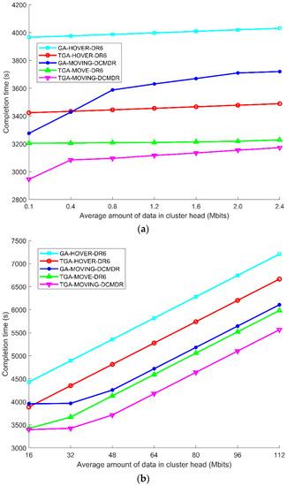
Figure 14. Completion time by the average amount of data of cluster heads. (a) Small amount of data cases; (b) large amount of data cases.

In small amount of data cases, as shown in Figure 14a, when the amount of data is very small, DCMDR has an obvious effect. With the increase in the amount of data, TGA has an obvious effect. Therefore, with the increase in the amount of data, the completion time of GA-MOVING-DCMDR is obviously more than that of TGA-HOVER-DR6. With the increase in the amount of data, the completion time of TGA-MOVE-DR6 changes slightly; because with DR6 mode, the small amount data can be transmitted rapidly, which has a slight impact on time. With TGA-MOVING-DCMDR, UAV can start gathering data from a long distance with the lower DRs and it has obvious advantages over other methods.

In large amount of data cases, as shown in Figure 14b, when the amount of data exceeds 32 Mbits, the completion time of all methods linearly increases with the amount of data obviously, because the UAV has to reduce flight speed or hover within the signal coverage of DR6, to complete the data gathering. The increased time is almost proportional to the increased amount of data.

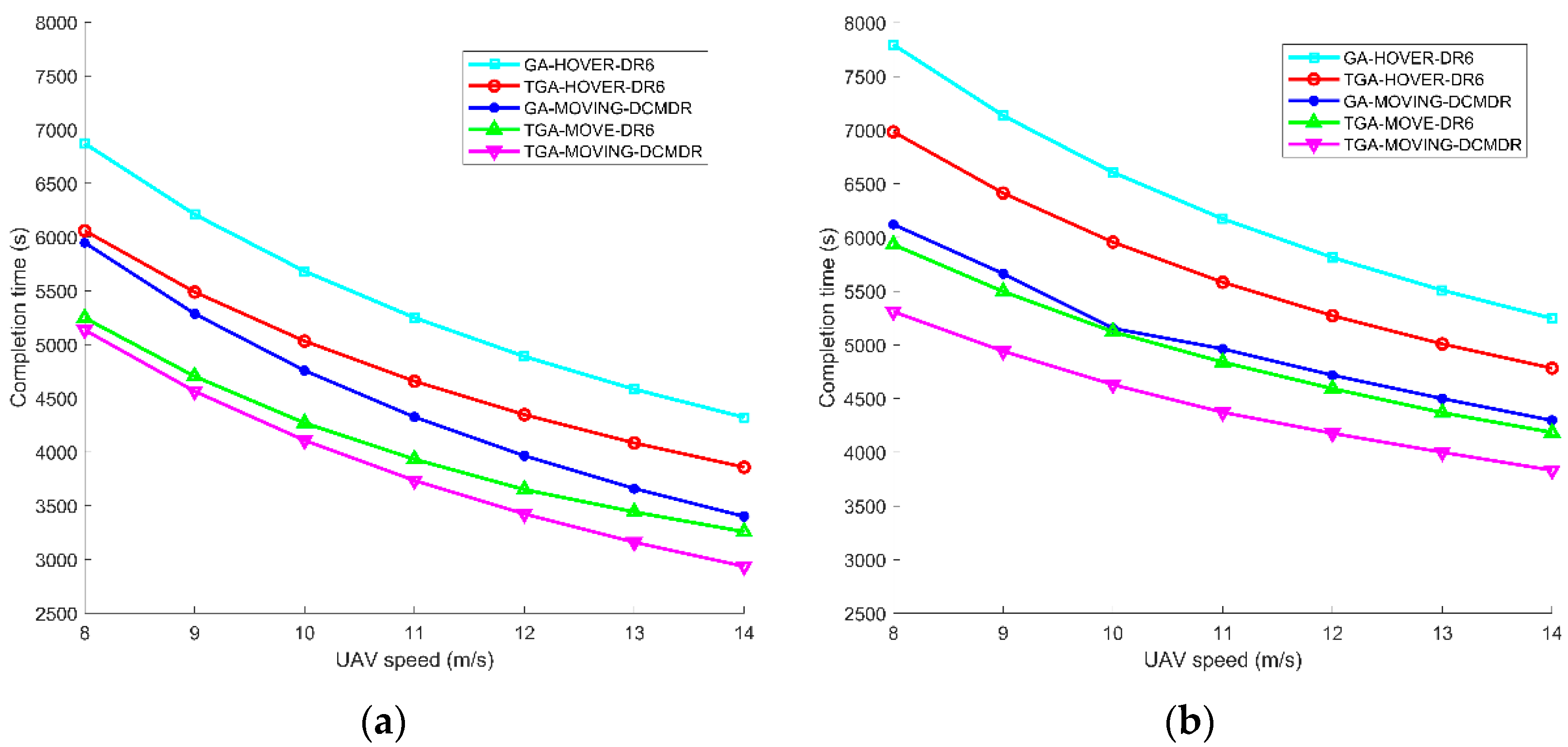
In scenario 2, we evaluated the influence of UAV speed on the completion time of the data collection task. The simulations of two cases were carried out, with the average data amount of cluster heads of 32 and 64 Mbits, respectively. In Figure 15, the completion time of the UAV data collection task decreases with the increase in the UAV speed, and the task completion time of the TGA-MOVING-DCMDR method is always the smallest in two data amount cases. Regarding TGA-MOVING-DCMDR, the difference in the completion time between the 64 Mbits case and 32 Mbits case increases with the increase in speed. This is because, within the signal coverage of DR6, the UAV hardly needs to reduce its speed in the 32 Mbits case, while it has to reduce its speed in the 64 Mbits case to complete the data gathering.

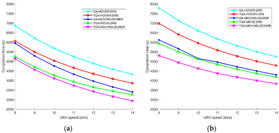
Figure 15. Completion time by UAV flight speed. (a) 32 Mbits; (b) 64 Mbits.

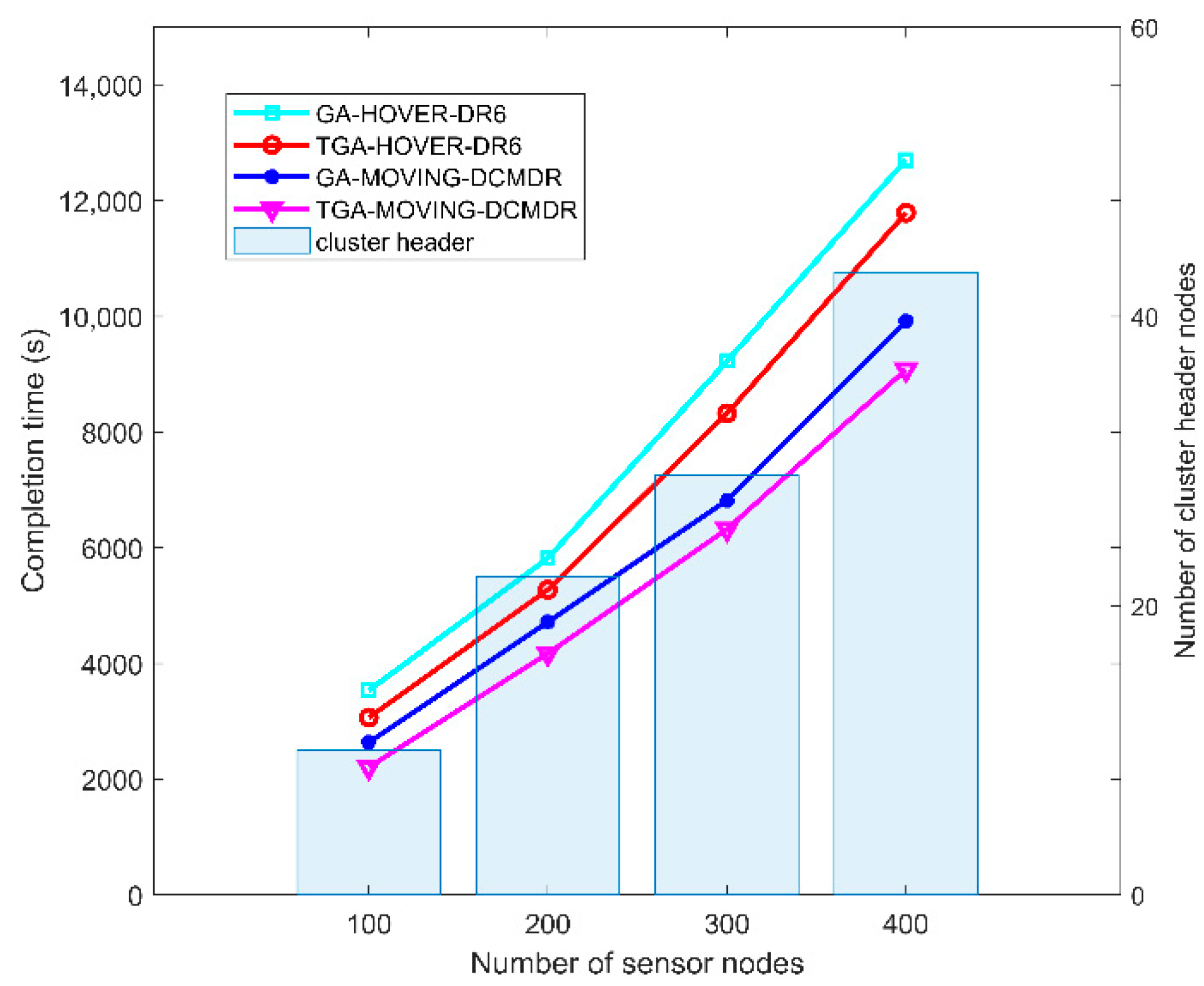
In scenario 3, we evaluated the performance of TGA-MOVING-DCMDR varying with sensor scale. We set the flying speed to 12 m/s, and the average amount of data in cluster heads was 64 Mbits. The scale of sensor nodes varies from 100 to 400. As shown in Figure 16, the number of cluster heads selected by ILEACH increases with the number of sensors, respectively, 13, 22, 30, 36, and the corresponding clustering ratios are 13%, 11%, 10%, and 9%. The completion time of the UAV data collection task in the four simulation groups increases with the number of sensor nodes. In the case of the same number of nodes, the completion time of the method TGA-MOVING-DCMDR is always less than the other three methods. The results show that the optimization scheme in this paper can be used in different scale scenarios.

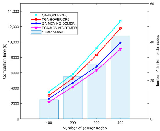
Figure 16. Completion time by number of sensor nodes.

5.2. Experiment

In order to verify the simulation results, we conducted real-world experiments, which were the same as the experimental scenes in Section 4. The battery capacity of UAV is limited, it can support flight time of 2000 s. As shown in Figure 17, the UAV with the LoRa 2.4 GHz dual-channel module and 6 cluster heads was deployed in a 5 × 5 km area, the UAV speed was set to 12 m/s, and the UAV planned path for data collection task was obtained using the TGA algorithm.

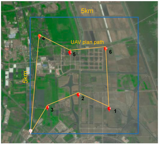
Figure 17. Real-world experiment site.

Regarding the task completion time, we first compared our TGA-MOVING-DCMDR with TGA-HOVER-DR6 and TGA-MOVE-DR6 methods for the large data amount stored in cluster heads. As can be seen in Table 5, for each data amount stored in cluster heads, the task completion time using the TGA-MOVING-DCMDR was less than those using the other two methods, which was basically consistent with the simulation status.

Table 5. UAV flight time comparison for higher data amount stored.

Methods	Cluster Head Data (Mbits)
	32	48	64	80	96	112
TGA-HOVER-DR6	1469	1584	1700	1815	1930	2045
TGA-MOVE-DR6	1257	1285	1404	1512	1631	1743
TGA-MOVING-DCMDR	1239	1251	1347	1472	1577	1692

Figure 18 shows the average packet loss ratio in the above experiments. The packet loss ratios of cluster heads were less than 3%, except for the fourth cluster head. It may be because the cluster head 4 was located in the bushes and surrounded by vegetation. In terms of packet loss ratio, the TGA-MOVING-DCMDR was similar to the other two methods, while the task completion time of our method is the lowest.

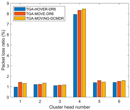
Figure 18. The packet loss ratios of cluster heads.

In practical systems, the cluster head sometimes stores a small amount of data. Therefore, we tested the task completion time of the UAV for the data amount within 1 Mbit stored in cluster heads. The results are shown in Table 6. TGA-HOVER-DR3 had the longest flight time for each amount of cluster head data, because DR3 is 14.27 kbit/s and the UAV can only collect data when hovering over the cluster head.

Table 6. UAV flight time comparison for lower data amount stored.

Methods	Cluster Head Data (Mbits)
	0.25	0.5	0.75	1.0
TGA-HOVER-DR3	1359	1491	1617	1743
TGA-HOVER-DR6	1240	1242	1245	1249
TGA-MOVE-DR3	1079	1105	1205	1301
TGA-MOVE-DR6	1165	1166	1168	1170
TGA-MOVING-DCMDR	1063	1082	1107	1136

With the increase in the amount of data, the completion time of TGA-HOVER-DR6 and TGA-MOVE-DR6 method barely changed, because DR6 is 1040 kbit/s, and the data transmitting time is much lower than the flight time. When the amount of data is less than 0.5 Mbits, the completion time of TGA-MOVE-DR3 is lower than that of TGA-MOVE-DR6. It is because the coverage area of DR6 is smaller than that of DR3, and the UAV can only receive signals at a short distance from the cluster head with DR6, while the TGA-MOVE-DR3 can start collecting data from a long distance. The task completion time of the TGA-MOVING-DCMDR was always the smallest with the same amount of data. Because it can adjust the data rate adaptively, when the amount of data is small, the data can be collected farther away from the cluster head.

6. Conclusions

In this paper, we proposed optimization schemes to solve the UAV data collection problems in remote areas without public networks. To reduce the UAV flight distance and time, the optimization schemes consist of three aspects. Specifically, the ILEACH algorithm was proposed, compared with the typical clustering algorithms (LEACH, TEEN, PEGASIS), it is aware of the distance from the cluster heads to UAV take-off point, while considering the factors of remaining energy, number of nodes covered, and average distance of neighbor nodes. Then, the TGA algorithm was presented to reduce the UAV planned path, which introduces the TLBO and local search optimization algorithms, and has a better convergence rate and path solution than those of GA. Finally, we proposed the DCMDR strategy, using LoRa 2.4 GHz technology with dual channels, and the data rate between UAV and cluster heads can be adaptively adjusted according to the distance and link quality. Compared with the current Sub-G LoRa technologies, it meets the requirement of high data rate while taking into account long-range communication.

Furthermore, we tested the thresholds of SNR, RSSI, and Distance for each DR through field tests in the Lingang area of Shanghai. When using the DCMDR scheme, with a flight speed of 4 m/s, up to 100 Mbits data in cluster head can be transmitted without UAV hovering and reducing speed.

Finally, we carried out simulations and experiments to verify the advantages of ILEACH and TGA-MOVING-DCMDR. In simulations with three classical datasets (R201, C201, and RC201), when the number of iterations was 200, the optimal solution and average solution of TGA for flight path were about two-thirds lower than those of GA. Compared with ILEACH-TGA, ILEACH-TGA can reduce the planned path distance by 30%. TGA-MOVING-DCMDR uses the minimum data gathering time regardless of the amount of data stored in the cluster heads. In small amount of data cases, it can start gathering data from a long distance with the lower DRs. In large amount of data cases, it can adjust the flight speed to complete the data gathering and reduce unnecessary flight distance. The experiments further verified the better performance of the optimization schemes, which can be applied to the UAV data collection problem well in remote areas without infrastructure. When using our schemes, with a flight speed of 12 m/s, up to 38 Mbits data in cluster head can be transmitted without UAV hovering and reducing speed.

For future work, the multi-UAV system will be considered for large area data collection. We will conduct more experiments with more end-nodes, algorithm complexity and energy efficiency will be further analyzed, to further evaluate the performance of the optimization scheme. The fixed wing drone, which has a much longer endurance and faster speed, will be studied to cover much larger areas.

References

- Chen, J.; Yan, F.; Mao, S.; Shen, F.; Xia, W.; Wu, Y.; Shen, L. Efficient data collection in large-scale UAV-aided wireless sensor networks. In Proceedings of the IEEE International Conference on WCSP, Xi’an, China, 23–25 October 2019; pp. 1–5. [Google Scholar]
- Ge, J.; Chao, F.; He, Z.; Shi, W. Research on Water Monitoring Information Acquisition System of UAV Based on Wireless Sensor Network. In Proceedings of the 11th International Conference on Modelling, Identification and Control, Tianjin, China, 13–15 July 2019; pp. 969–977. [Google Scholar]
- Tao, M.; Li, X.; Yuan, H.; Wei, W. UAV-Aided trustworthy data collection in federated-WSN-enabled IoT applications. Inf. Sci. 2020, 532, 155–169. [Google Scholar] [CrossRef]
- Carcelle, X.; Heile, B.; Chatellier, C.; Pailler, P. Next WSN applications using ZigBee. In Home Networking; Springer: Boston, MA, USA, 2008; pp. 239–254. [Google Scholar]
- Bembe, M.; Abu-Mahfouz, A.; Masonta, M.; Ngqondi, T. A survey on low-power wide area networks for IoT applications. Telecommun. Syst. 2019, 71, 249–274. [Google Scholar] [CrossRef]
- Sinha, R.S.; Wei, Y.; Hwang, S.-H. A survey on LPWA technology: LoRa and NB-IoT. Ict Express 2017, 3, 14–21. [Google Scholar] [CrossRef]
- Behjati, M.; Noh, A.M.; Alobaidy, H.; Zulkifley, M.; Nordin, R.; Abdullah, N. LoRa Communications as an Enabler for Internet of Drones towards Large-Scale Livestock Monitoring in Rural Farms. Sensors 2021, 21, 5044. [Google Scholar] [CrossRef] [PubMed]
- Choi, C.-S.; Baccelli, F.; De Veciana, G. Modeling and Analysis of Data Harvesting Architecture Based on Unmanned Aerial Vehicles. IEEE Trans. Wirel. Commun. 2019, 19, 1825–1838. [Google Scholar] [CrossRef] [Green Version]
- Gallego-Madrid, J.; Molina-Zarca, A.; Sanchez-Iborra, R.; Bernal-Bernabe, J.; Santa, J.; Ruiz, P.; Skarmeta-Gómez, A. Enhancing Extensive and Remote LoRa Deployments through MEC-Powered Drone Gateways. Sensors 2020, 20, 4109. [Google Scholar] [CrossRef]
- Saraereh, O.A.; Alsaraira, A.; Khan, I.; Uthansakul, P. Performance Evaluation of UAV-Enabled LoRa Networks for Disaster Management Applications. Sensors 2020, 20, 2396. [Google Scholar] [CrossRef]
- Zhang, M.; Li, X. Drone-Enabled Internet-of-Things Relay for Environmental Monitoring in Remote Areas Without Public Networks. IEEE Internet Things J. 2020, 7, 7648–7662. [Google Scholar] [CrossRef]
- Hung, C.-C.; Hsieh, C.-C. Big data management on wireless sensor networks. In Big Data Analytics for Sensor-Network Collected Intelligence; Elsevier: Amsterdam, The Netherlands, 2017; pp. 99–116. [Google Scholar]
- Sun, G.; Li, J.; Liu, Y.; Liang, S.; Kang, H. Time and Energy Minimization Communications Based on Collaborative Beamforming for UAV Networks: A Multi-Objective Optimization Method. IEEE J. Sel. Areas Commun. 2021, 39, 3555–3572. [Google Scholar] [CrossRef]
- Babu, N.; Virgili, M.; Papadias, C.B.; Popovski, P.; Forsyth, A.J. Cost-and Energy-Efficient Aerial Communication Networks with Interleaved Hovering and Flying. IEEE Trans. Veh. Technol. 2021, 70, 9077–9087. [Google Scholar] [CrossRef]
- Rao, R.V.; Savsani, V.J.; Vakharia, D.P. Teaching–learning-based optimization: A novel method for constrained mechanical design optimization problems. Comput. Aided Des. 2011, 43, 303–315. [Google Scholar] [CrossRef]
- Karunanithy, K.; Velusamy, B. Energy efficient cluster and travelling salesman problem based data collection using WSNs for Intelligent water irrigation and fertigation. Measurement 2020, 161, 107835. [Google Scholar] [CrossRef]
- Ho, D.-T.; Grøtli, E.I.; Sujit, P.; Johansen, T.A.; Sousa, J.B. Optimization of wireless sensor network and UAV data acquisition. J. Intell. Robot. Syst. 2015, 78, 159–179. [Google Scholar] [CrossRef]
- Wang, G.; Lee, B.-S.; Ahn, J.Y. UAV-assisted cluster head election for a UAV-based wireless sensor network. In Proceedings of the IEEE 6th International Conference on Future Internet of Things and Cloud, Barcelona, Spain, 6–8 August 2018; pp. 267–274. [Google Scholar]
- Alemayehu, T.S.; Kim, J.-H. Efficient Nearest Neighbor Heuristic TSP Algorithms for Reducing Data Acquisition Latency of UAV Relay WSN. Wirel. Pers. Commun. 2017, 95, 3271–3285. [Google Scholar] [CrossRef]
- Alemayehu, T.S.; Kim, J.-H.; Yoon, W. Fault-Tolerant UAV Data Acquisition Schemes. Wirel. Pers. Commun. 2020, 114, 1669–1685. [Google Scholar] [CrossRef]
- Xiao-Ting, J.; Hai-Bin, X.; Li, Z.; Sheng-De, J. Flight path planning based on an improved genetic algorithm. In Proceedings of the Third International Conference on Intelligent System Design and Engineering Applications, Hong Kong, China, 16–18 January 2013; pp. 775–778. [Google Scholar]
- Yang, T.; Hu, Y.; Yuan, X.; Mathar, R. Genetic algorithm based UAV trajectory design in wireless power transfer systems. In Proceedings of the IEEE Wireless Communications and Networking Conference, Marrakesh, Morocco, 15–18 April 2019; pp. 1–6. [Google Scholar]
- Nasution, T.H.; Siregar, I.; Yasir, M. UAV telemetry communications using ZigBee protocol. J. Phys. Conf. Ser. 2017, 914, 012001. [Google Scholar] [CrossRef]
- Yu, L.; Fei, Q.; Geng, Q. Combining Zigbee and inertial sensors for quadrotor UAV indoor localization. In Proceedings of the IEEE International Conference on Control and Automation, Hangzhou, China, 12–14 June 2013; pp. 1912–1916. [Google Scholar]
- Khalifeh, A.F.; AlQudah, M.; Tanash, R.; Darabkh, K.A. A simulation study for UAV-aided wireless sensor network utilizing ZigBee protocol. In Proceedings of the 14th International Conference on Wireless and Mobile Computing, Networking and Communications (WiMob), Limassol, Cyprus, 15–17 October 2018; pp. 181–184. [Google Scholar]
- Sidek, O.; Abdullah, A.; Za'bah, U.; Amran, N.; Jafar, H.; Hadi, M.A.; Nikmat, F.; Halim, Z.; Mansor, M. Development of prototype system for monitoring and computing greenhouse gases with unmanned aerial vehicle (uav) deployment. In Proceedings of the International Symposium on Technology Management and Emerging Technologies, Bandung, Indonesia, 27–29 May 2014; pp. 98–101. [Google Scholar]
- Tan, Z.; Yang, X.; Pang, M.; Gao, S.; Li, M.; Chen, P. UAV-Assisted Low-Consumption Time Synchronization Utilizing Cross-Technology Communication. Sensors 2020, 20, 5134. [Google Scholar] [CrossRef]
- Augustin, A.; Yi, J.; Clausen, T.; Townsley, W.M. A Study of LoRa: Long Range & Low Power Networks for the Internet of Things. Sensors 2016, 16, 1466. [Google Scholar]
- Wendt, T.; Volk, F.; Mackensen, E. A benchmark survey of long range (LoRaTM) spread-spectrum-communication at 2.45 GHz for safety applications. In Proceedings of the 16th Annual Wireless and Microwave Technology Conference (IEEE WAMICON), Cocoa Beach, FL, USA, 13–15 April 2015; pp. 1–4. [Google Scholar]
- Trasviña-Moreno, C.A.; Blasco, R.; Casas, R.; Asensio, A. A network performance analysis of LoRa modulation for LPWAN sensor devices. In Ubiquitous Computing and Ambient Intelligence; Springer: Cham, Switzerland, 2016; pp. 174–181. [Google Scholar]
- Kim, D.K.; Son, H.S.; Yang, S.H. LoRa Communication and Smartphone Technology to Share Locations of Drones. Trans. Korean Soc. Mech. Eng. A 2019, 43, 903–909. [Google Scholar] [CrossRef]
- da Silva, R.I.; Nascimento, M.A. On best drone tour plans for data collection in wireless sensor network. In Proceedings of the 31st annual ACM Symposium on Applied Computing, Pisa, Italy, 4–8 April 2016; pp. 703–708. [Google Scholar]
- Rezende, J.D.C.V.; Da Silva, R.I.; Souza, M.J.F. Gathering Big Data in Wireless Sensor Networks by Drone. Sensors 2020, 20, 6954. [Google Scholar] [CrossRef]
- Lawler, E.L.; Lenstra, J.K.; Kan, A.R.; Shmoys, D.B. The Traveling Salesman Problem: A Guided Tour of Combinatorial Optimization; Wiley: New York, NY, USA, 1985. [Google Scholar]
- Heinzelman, W.R. Energy-efficient communication protocol for wireless microsensor networks. In Proceedings of the 33rd Annual Hawaii International Conference on System Sciences, Maui, HI, USA, 7 January 2000. [Google Scholar]
- Manjeshwar, A.; Agrawall, D.P. TEEN: A routing protoeol for enhanced efficiency in wireless sensor networks. In Proceedings of the 15th Parallel and Distributed Proeessing Symposium, San Francisco, CA, USA, 23–27 April 2001. [Google Scholar]
- Lindsey, S.; Raghavendra, C.S. PEGASIS: Power Efficient Gathering in Sensor Information Systems. In Proceedings of the IEEE Aerospace Conference, Big Sky, MT, USA, 9–16 March 2002; Volume 3, pp. 1130–1152. [Google Scholar]
- Moghaddam, B.F.; Ruiz, R.; Sadjadi, S.J. Vehicle routing problem with uncertain demands: An advanced particle swarm algorithm. Comput. Ind. Eng. 2012, 62, 306–317. [Google Scholar] [CrossRef] [Green Version]
- Dorigo, M.; Maniezzo, V.; Colorni, A. Ant system: Optimization by a colony of cooperating agent. IEEE Trans. Syst. Man Cybern. Part B-Cybern. 1996, 26, 29–41. [Google Scholar] [CrossRef] [PubMed] [Green Version]
- Gu, Z.; Zhu, Y.; Wang, Y.; Du, X.; Guizani, M.; Tian, Z. Applying artificial bee colony algorithm to the multidepot vehicle routing problem. Softw. Pract. Exp. 2020, 52, 756–771. [Google Scholar] [CrossRef]
- Wang, C.L.; Li, S.W. Hybrid fruit fly optimization algorithm for solving multi-compartment vehicle routing problem in intelligent logistics. Adv. Prod. Eng. Manag. 2018, 13, 466–478. [Google Scholar] [CrossRef]
- Tao, Y.; Wang, F. An effective tabu search approach with improved loading algorithms for the 3L-CVRP. Comput. Oper. Res. 2015, 55, 127–140. [Google Scholar] [CrossRef]
- Zarandi, M.H.F.; Hemmati, A.; Davari, S.; Turksen, I.B. A simulated annealing algorithm for routing problems with fuzzy constrains. J. Intell. Fuzzy Syst. 2014, 26, 2649–2660. [Google Scholar] [CrossRef] [Green Version]
- SINTEF Research Institutes. Solomon Benchmark Datasets (R201, C201, and RC201). Available online: https://www.sintef.no/projectweb/top/vrptw/solomon-benchmark/ (accessed on 19 December 2021).
Publisher’s Note: MDPI stays neutral with regard to jurisdictional claims in published maps and institutional affiliations. |
© 2022 by the authors. Licensee MDPI, Basel, Switzerland. This article is an open access article distributed under the terms and conditions of the Creative Commons Attribution (CC BY) license (https://creativecommons.org/licenses/by/4.0/).