Abstract
Small fixed-wing electric Unmanned Aerial Vehicles (UAVs) are perfect candidates to perform tasks in wide areas, such as photogrammetry, surveillance, monitoring, or search and rescue, among others. They are easy to transport and assemble, have much greater range and autonomy, and reach higher speeds than rotatory-wing UAVs. Aiming to contribute towards their future implementation, the objective of this article is to benchmark commercial, small, fixed-wing, electric UAVs and compatible RGB cameras to find the best combination for photogrammetry and data acquisition of mussel seeds and goose barnacles in a multi-region intertidal zone of the south coast of Galicia (NW of Spain). To compare all the options, a Coverage Path Planning (CPP) algorithm enhanced for fixed-wing UAVs to cover long areas with sharp corners was posed, followed by a Traveling Salesman Problem (TSP) to find the best route between regions. Results show that two options stand out from the rest: the Delair DT26 Open Payload with a PhaseOne iXM-100 camera (shortest path, minimum number of pictures and turns) and the Heliplane LRS 340 PRO with the Sony Alpha 7R IV sensor, finishing the task in the minimum time.
1. Introduction
The Galician coast (NW region of Spain) is characterized by its flooded river valleys, called rías [1,2,3,4]. They offer ideal conditions for fishing and shellfish activities due to their unique properties, such as bathymetry, water temperature, big tides, strong ocean currents and, especially, the upwelling phenomenon, that allows cold, nutrient-rich water to rise from depths, causing the blooming of phytoplankton [1,2,3,4,5,6]. In this Spanish region, shellfish harvesting has historically been a marginal activity without administrative control, characterized by a lack of technology, high manual labor, and feminization [3]. Nevertheless, it has traditionally provided sociocultural benefits, reflected in physical and cognitive interactions between humans and nature since prehistoric times, and supplemental economic benefits for household incomes [3].
Two types of shellfish of special interest coexist in the rocks of the intertidal space of the Galician coast. On the one hand, the mussel (Mytilus galloprovincialis) seed is collected from the rocks and attached to culture ropes until the commercial size is reached [7]. Galicia is the main mussel producer in Europe and one of the first in the world [2], representing 12% of worldwide production in 2018 [5]. On the other hand, the goose barnacle (Pollicipes pollicipes) is the most important economic resource extracted directly from the rocks of the northern coast of Spain and mainland Portugal [8].
In recent decades, the shell fishing capacity in Galicia has decreased, with 13% fewer boats, 10% less capacity, and half of the on-foot shell fishers [3]. Anthropogenetic pressures such as overfishing, poaching, pollution or climate change negatively influence their habitats and populations [3,9]. Moreover, despite the socioeconomic importance of shellfish harvesting, there are few studies, dating from 1993 and reaching 98 publications by 2017, yielding a problematic lack of statistics and economic data [3].
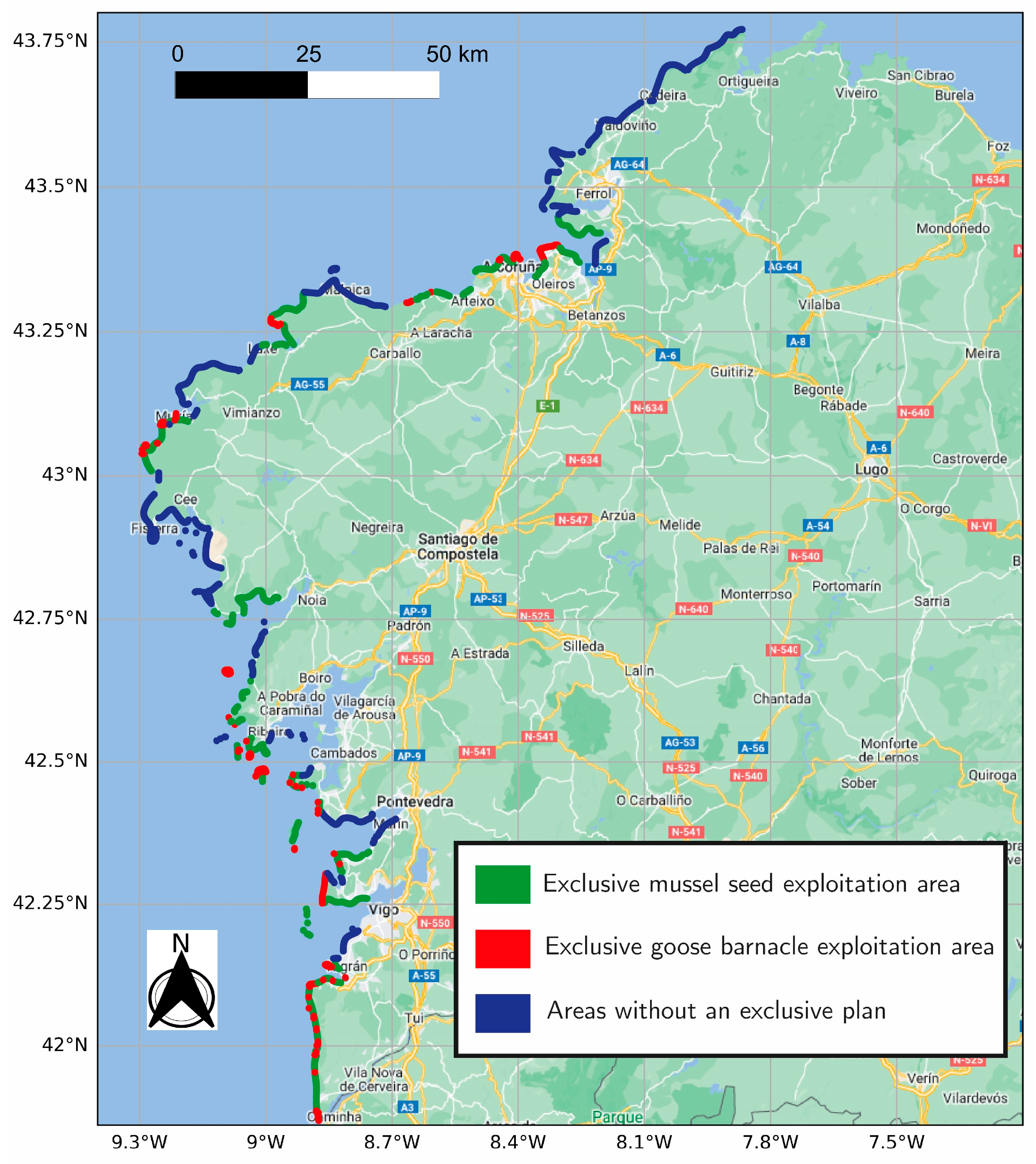
Regarding the specific case of mussels and goose barnacles, problems are exacerbated since they coexist in the same habitats and their harvesting methods are very rough and manual. Goose barnacles are separated from rocks using scrapers and after that, shell fishers select those that have reached commercial size, discarding undersized barnacles and inadvertent captures of other organisms [10]. On the other hand, while mussel extraction is carried out, barnacles are also affected, which is one of the possible aggravating factors in the depletion of this species [3]. For these reasons, the Consellería do Mar (Ministry of the Sea), dependent on the regional government of the Xunta de Galicia, has developed a plan to guarantee exclusive exploitation areas for mussel seed and goose barnacles (see Figure 1).
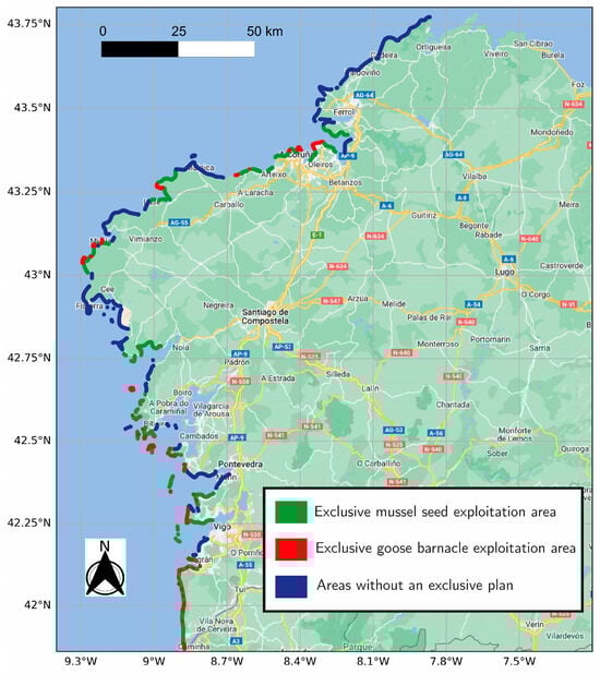
Figure 1.
Galician coastline map. Exclusive mussel seed exploitation areas (green). Exclusive goose barnacle exploitation areas (red). Areas without an exclusive plan (blue) [11].
All these factors call for further research and data collection to generate ecological models for enhancing the execution of conservation strategies. However, it is not an easy task in intertidal spaces. In addition to the large extension of monitoring and its complicated access, there are also challenges related to the small size of the organisms and the available time for sampling, which is limited to low tide intervals (around two hours). Thus, one of the determining factors for a good study would be the rapid collection of data in large areas with the highest resolution possible [9]. Traditionally, researchers have collected samples and conducted field experiments. The most common techniques are rather small quadrats and photographic surveys (less than 1 m2), but large-area patterns of species distributions are lost. For monitoring and mapping on a broader scale, satellite imagery and manned aerial platforms have also been used, but low fine-grained spatial details cannot be captured [9]. At this point, the use of UAVs is of great help for the study of marine environments since they present a high resolution by being able to perform low flights while covering wide areas, especially fixed-wing UAVs. For example, in [12], a general overview of the use of UAVs as a survey tool for marine mammal studies is presented, using in several cases fixed-wing vehicles. In [13], authors propose the use of a fixed-wing UAV for meteorology research in oceans. In [14], another fixed-wing UAV was used for coastal assessment and management, creating Digital Surface Models (DSM) through photogrammetry techniques.
In [9], a rotatory-wing UAV was used to cover eight intertidal areas in Portugal to estimate mussel demographic parameters. From each region, an orthophoto mosaic, a Digital Elevation Model (DEM), a terrain roughness index raster image and a classified mosaic based on the following land-cover classes: water, sand, rocks, mussels, algae and urban, were obtained. Rotatory-wing UAVs were also used for automating coral reef assessment [15], fauna monitoring and shark surveillance [16], sensitive marine habitat mapping and classification [17], underwater benthic monitoring and mapping [18], intertidal mudflat mapping [19], mussel distribution [20], and macroalgae monitoring [21,22,23], among others, but all of them follow the same pattern: either the resolution is low or the study area is small. Due to the great length of the Galician coastline (more than 1500 km [24]) and the short time of low tides for data collection, this work proposes the use of a small fixed-wind electric UAV for this type of operation. Small fixed-wing UAVs are relatively easy to transport and assemble; they can also carry larger payloads and reach higher speeds and flight ranges [25,26,27,28,29].
Furthermore, because of the importance of covering all the inspection areas in the minimum possible time, it is crucial to plan the mission carefully. Mathematically, this is considered a Traveling Salesman Problem (TSP) to determine the order in which all the regions must be visited, coupled with a Coverage Path Planning (CPP) solution to efficiently cover each region [30,31,32]. Both the TSP and the CPP are already NP-hard problems separately. However, they must be nested to obtain the optimal solution, making it necessary to determine the points where UAVs must enter and exit each region, making this problem even more complex [30,31,32].
The CPP allows to explore all the locations in a region of interest, considering vehicle restrictions, sensor characteristics and avoiding obstacles [25,27,33,34,35,36]. The CPP is a task that has had multiple applications in robotics for a long time, like vacuum cleaner robots, lawn mowers, painting robots, demining, and agriculture [35,36], among many others. In the field of UAVs, it is also a very common solution. In [36], it is implemented for optimal coverage in a port environment. In [27], CPP is used in photogrammetry tasks with a fixed-wing UAV, where turning radius constraints are considered. Turning constraints in fixed-wing CPP problems are also studied in [26,33,37,38]. Other labors regarding the CPP problem in UAVs are search and rescue (SAR), mapping, precision agriculture, infrastructure inspection and surveillance [26,39].
CPP algorithms can be classified as (i) heuristics, which may not guarantee full coverage, or (ii) complete methods, guaranteeing full coverage [25,35,40]. Heuristic algorithms are based on simple rules and random approaches that define UAV behavior and, despite not guaranteeing full coverage, they may have some advantages in search or exploration applications from a cost/benefit point of view [25,35,40]. Complete algorithms are usually based on the decomposition of the area of interest into polygonal subregions called cells [25,27,35,37]. This decomposition can be (i) exact if the re-union of the cells forms the original region [33,36,38,41,42,43] or (ii) approximate (also called grid-based) [25,27,34,35]. Approximate decomposition techniques usually take as cell dimensions a proportional value of the sensor size with a square, hexagonal, or triangular shape [25,27,34,35]. Approximate decomposition algorithms are often used in indoor or small regions, being more suitable for rotatory-wing UAVs because they tend to generate sharper turns and more erratic paths, need very precise localization to maintain map coherency, and memory usage during calculations grows exponentially [27,35].
Exact decomposition methods are based on converting concave, complex polygons into simple, non-overlapping, convex subregions and, on these areas, applying a simple CPP algorithm, with the Back-and-Forth patterns (BF), such as the Boustrophedon and the trapezoidal pattern [33,34,36,37,42], and spiral patterns [26,36] being the most typical ones. All these patterns are encompassed in a more general classification called Morse-based algorithms [33,35,37,42].
For BF patterns, it is necessary to find the optimal direction of each cell that reduces the number of turns of the UAV. When there is a single non-complex cell, the two main methods are the rotating caliper and vertex perpendicular methods [36]. Then, the optimal sweep direction is considered parallel to the minimum width direction [27,36,44,45]. When the region is more complicated, it must be previously decomposed, making it necessary to establish a sweep direction for each sub-region according to the principle of minimum sum of widths [33,36,44,45].
Besides, in some works, researchers have tried to reunify some convex sub-regions when they fulfilled a series of common features, as having too many convex partitions could result in cumbersome and inefficient results [33,36,43].
Finally, to determine the order in which the sub-regions must be visited, the problem can be transformed into a TSP [26,33,36,41]. The TSP can be solved by several algorithms to obtain efficient path planning. Some of the most popular in literature are the metaheuristic algorithms (Particle Swarm Optimization (PSO) [46,47], Genetic Algorithms (GA) [26,36,41,48], Ant Colony Optimization (ACO) [34,49], or the Firefly Algorithm (FA) [46]), the Christofides Algorithm [50], or the Dynamic Programming Formulation [44].
The main aim of this article is to carry out benchmarking between various models of commercial small fixed-wing electric UAVs with different combinations of RGB cameras in order to determine which is most suitable for photogrammetry and goose barnacle and mussel seed data acquisition. The simulation scenario is composed of 15 areas in an intertidal zone of the Galician coast. An Exact Cellular Decomposition method adapted to long areas for fixed-wind UAVs is implemented before applying a Boustrophedon CPP algorithm in each cell. Finally, the centroids of each cell are calculated, transforming them into a TSP problem that is solved by a PSO algorithm. Notice that the TSP and CPP are implemented separately. This is since we are focused on benchmarking some UAV and camera models instead of looking for the more accurate and optimal route and, as a first approach to simplify the problem and reduce the computational time, it is enough.
The CPP is used to compare the performance of each sensor and UAV within the regions of interest according to the following parameters: (i) traveled distance within the regions, (ii) time employed for assessing all the regions, (iii) number of pictures taken, and (iv) number of turnings generated by the sweep patterns of the BF algorithm.
The remainder of the article is divided as follows: in Section 2, the selection of the cameras, UAVs, study areas and algorithms are introduced, explaining an enhanced method for merging cells in long regions with sharper corners for fixed-wing UAVs. In Section 3, the simulation results of all the possible combinations of UAVs and cameras are shown, obtaining two combinations that stand out from the rest: the Delair DT26 Open Payload with a PhaseOne iXM-100 sensor and the Heliplane LRS 340 PRO with a Sony Alpha 7R IV camera. In Section 4, a final discussion where the main results are presented is realized, including why the DT26 Open Payload could be the best option for this operation. Finally, Section 5 presents the conclusions.
2. Materials and Methods
2.1. Cameras
First, a compilation of cameras is made, considering the following specifications: resolution, sensor size, focal length, and continuous shooting rate. These features directly impact key mission parameters such as Field of View (FOV), flight altitude, and the maximum UAV speed. The main objective is to guarantee that these properties yield a Ground Sampling Distance (GSD) adequate for distinguishing shellfish from other organisms and the rocky background, while also enabling the required image overlap for 3D photogrammetry reconstructions and maintaining a safe flight altitude. In addition, it is crucial to estimate the total weight and dimensions of the camera, lens, and auxiliary equipment to know whether an UAV model can carry the system or not.
The following cameras have passed this first screening: Sony Alpha 7R IV, Sony RX1RII, Imperx T9040, and PhaseOne iXM-100, although the study was much wider. PhaseOne iXM-RS280F and PhaseOne iXM-RS150F, despite having higher resolution and achieving a lower GSD, are too heavy. The PhaseOne iXM-50 is similar in weight and dimensions to the PhaseOne iXM-100, but its resolution is halved. The ADTi Surveyor MAX 61S, DJI H20, Canon EOS 5D Mark IV, Canon M6 Mark II, and Canon EOS R100 have a significantly lower FOV than the selected cameras. Finally, the DJI P1, Nikon Z8, Nikon Z9 and Nikon D850 do not ensure a sufficient continuous shooting rate.
In Table 1, the main characteristics of the chosen cameras are summarized. Although the focal length may vary depending on the selected lens and camera configuration, real fixed values are set to guarantee a minimum flight altitude of 60 m to limit bird interactions [51] and other possible hazards such as buildings, trees, electrical towers, or antennas.

Table 1.
Main characteristics of the selected cameras.
In Table 2, some important properties needed for aerial photogrammetry, calculated from Table 1, are shown. To complete Table 2, it is considered a GSD of 0.8 cm/pix, as in [9], researchers used this value for identifying mussels on rocks, and a forward and side overlaps of 80% and 75%, respectively. These overlap values were established to compare all the cameras in the same circumstances and maintain a reasonable and realistic estimation according to previous studies [9,58,59].
Table 2.
Calculated properties of the chosen cameras needed for aerial photogrammetry from a GSD value of 0.8 cm/pix, a frontal overlap of 80% and a side overlap of 75%.
2.2. Commercial Small Fixed-Wing Electric UAVs
As in the previous subsection, a comprehensive search on commercial small fixed-wing electric UAVs is carried out. The main parameters considered are the following: operation range and time, cruise speed, maximum payload weight and camera compatibility. The chosen UAVs are shown in Table 3 with their main properties.
Table 3.
Selected UAVs with their main characteristics of interest. For DELTAQUAD PRO #MAP and Heliplane LRS340 PRO where two values are shown, the first one corresponds to the Sony Alpha 7R IV and the second one to the Sony RX1RII.
Other models have been analyzed. WingtraOne GEN II, Delair UX11, SCR Tucan, the Marlyn by AtmosUAV, Quantix Mapper and the eBee X by SenseFly have too low autonomy or range; the Heliplane LRS240 PRO is similar to the Heliplane LRS340 PRO but with smaller wings and, hence, less weight; but the reduction in its size negatively affects its flight range and time [64], and PUMA LE incorporates an integrated camera designed for battlefield environments that does not fit in this problem [66].
2.3. Detailed Work Scenario
For the benchmarking, a small area of the south Galician coast is selected, specifically the northern area controlled by the association of fishermen of Baiona. The map images of the zone presented in [11] are georeferenced and converted into orthophotos in QGIS [67]. Then, the regions of interest are approximated by 15 polygons (see Figure 2). These regions, with a total area of 1.31 km2, are where UAV and camera performances will be compared.
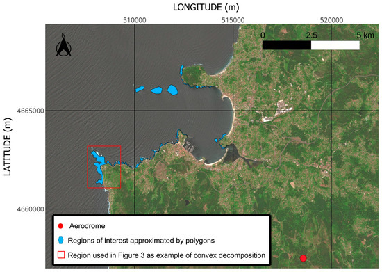
Figure 2.
Polygonised areas and aerodrome location (WGS 84/UTM ZONE 29N).
In addition, all UAVs take-off and land at the aerodrome of the Val Miñor Aeromodeling Club, located approximately 8 km southwest of Baiona (see Figure 2). For safety reasons, it was considered that they must land with at least 20% of battery. Therefore, if they cannot cover all the areas in one flight, they must go to the aerodrome to change their batteries and go back to the working scenario. Finally, it is crucial to emphasize that the inspection can only be carried out during low tides, as high tides can submerge the areas being surveyed, hampering photogrammetry results. For this purpose, a two-hour working window is established, starting one hour before low tide and ending one hour after. Although some UAV models have autonomy greater than two hours, the effective inspection time is constrained to this working window.
2.4. Coverage Path Planning (CPP) Algorithm
As can be appreciated in Figure 2, polygon contours are irregular and have numerous concave corners, except those representing the islands. Due to the complexity of the problem and the use of fixed-wing UAVs, an Exact Cellular Decomposition is carried out [27,35]. Each region of interest is decomposed, extending the edges of the polygon that form an interior angle greater than 180 degrees, until they hit another edge of the original polygon [33]. Let be a random vertex of the polygon, the next vertex clockwise and the previous vertex clockwise, applying the cross product of vectors [43] defined as:
with a vector of the form ; if , then the vertex is concave; if , the vertex is convex; and if , vertices are collinear.
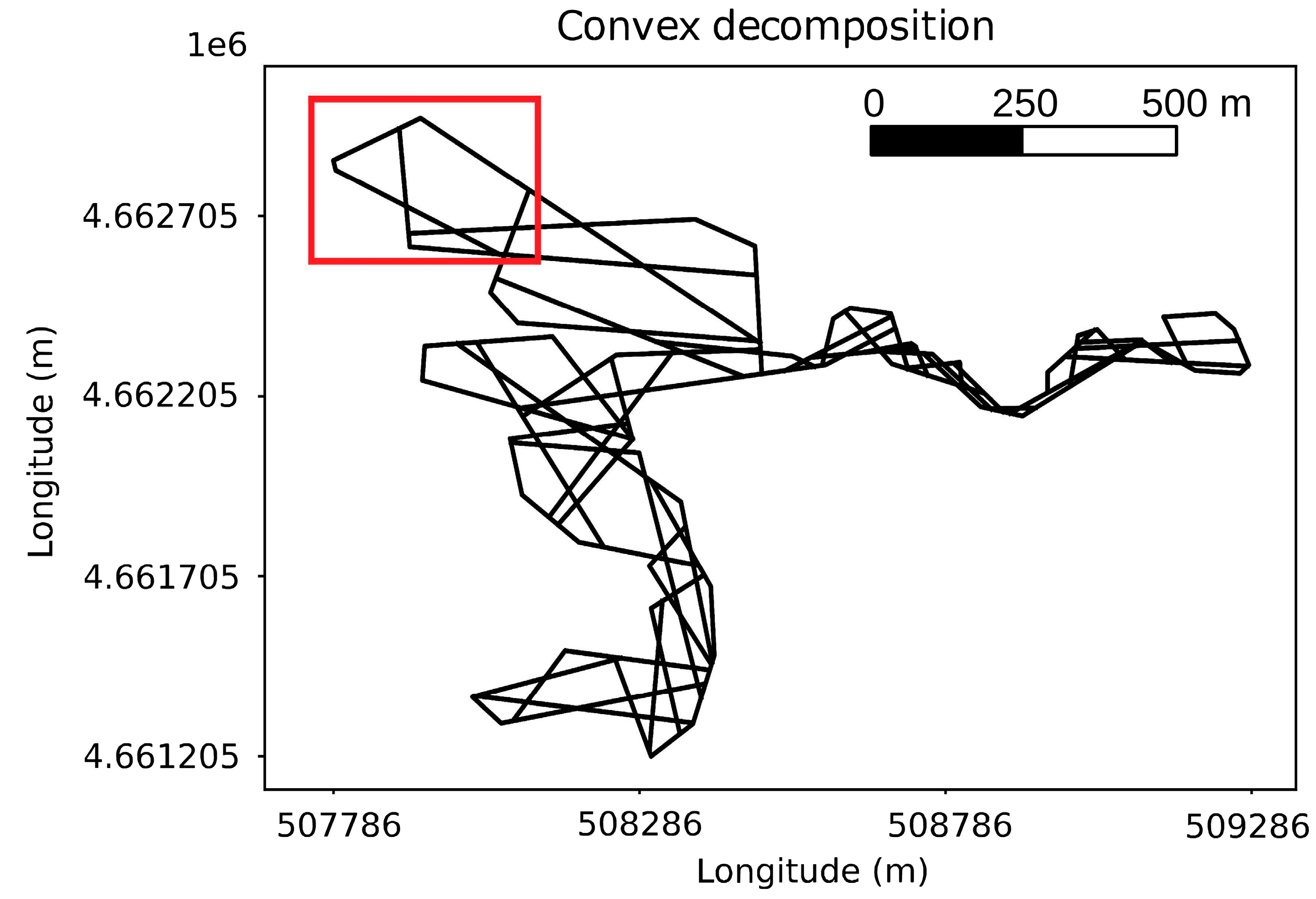
As an example, the highlighted leftmost polygon in Figure 2 is considered; 39 out of the 88 vertices of this area are concave. After applying the division criteria explained above, a total of 146 polygonal sub-regions, called cells, are obtained (see Figure 3).
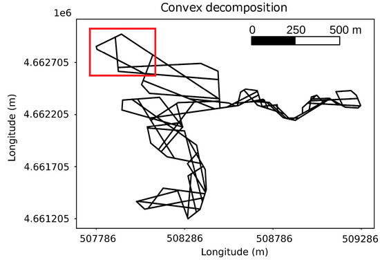
Figure 3.
Example of the convex decomposition in a polygon.
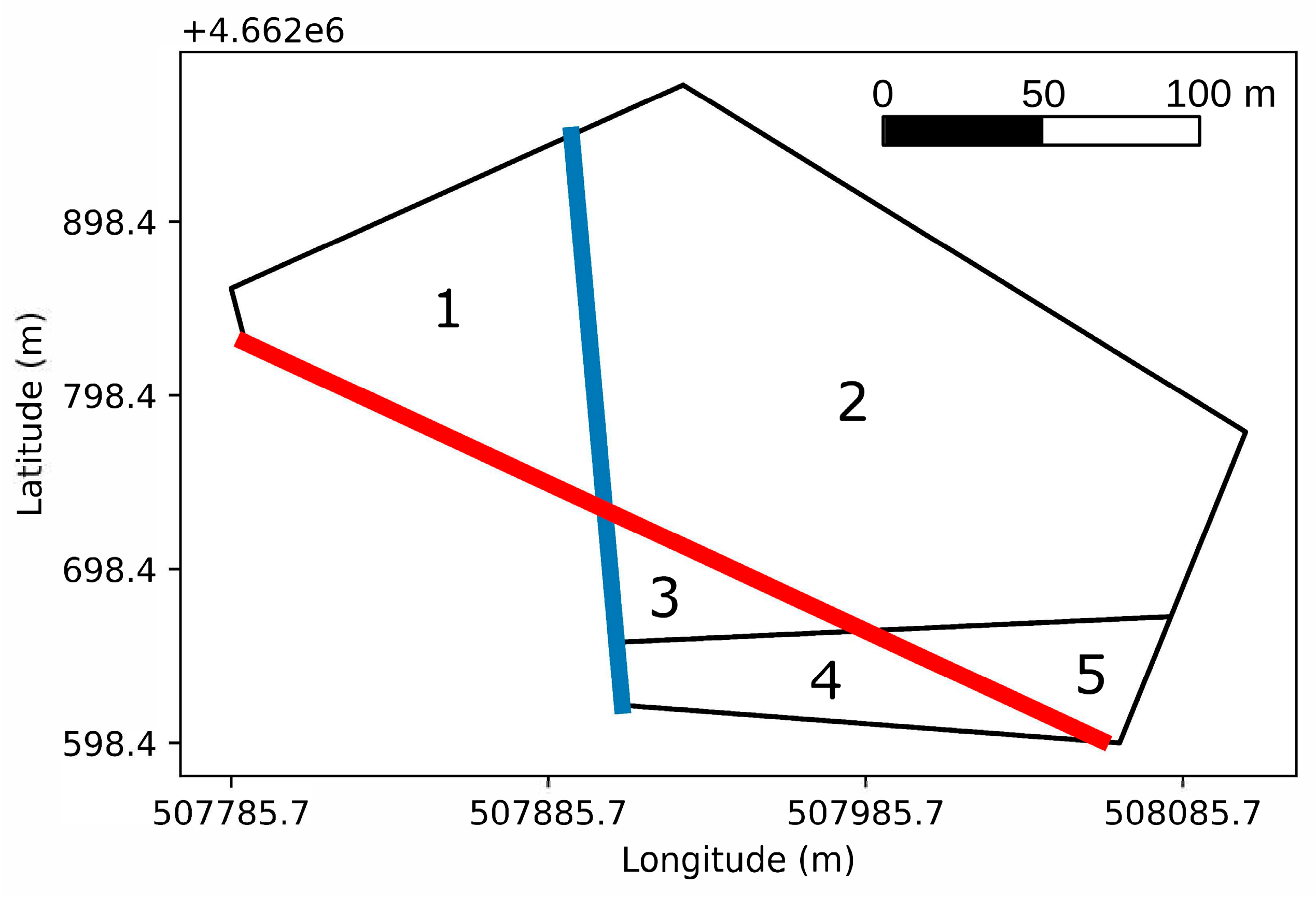
If UAV routes were determined according to this result, they would be inefficient and hard to cover successfully. For this reason, adjacent sub-regions are merged in two stages. In the first one, cells can be merged if their final combination does not form any concave interior angle. However, comparing all cell combinations becomes cumbersome, as it was already proved in [33]. To speed up the calculations, adjacent cells were previously determined. In addition, an extra condition must be fulfilled: if two merged cells create a concave interior angle belonging to a vertex of the original non-splitting polygon, they must remain separated, and the algorithm discards this option. For example, in Figure 4, if sub-regions 1 and 2 are merged, sub-region 5 is the only possibility to increment the size of the sub-polygon, as sub-region 3 forms an interior concave angle with sub-region 1 belonging to the original non-splitting polygon.

Figure 4.
Example of the possible merged sub-polygons extracted from the uppermost part of Figure 3. In red: {1,2,5}–{3,4}. In blue: {1}–{2,3,4,5}. (WGS84/UTM 29N).
Notice that this is a small case where there are only two possibilities to merge the sub-regions (red and blue in Figure 4). However, when a bigger polygon is decomposed, the number of options can increase considerably, making it computationally unaffordable to continue solving the problem. Then, before carrying on with the sub-polygon simplification, the minimum sum of the widths of each combination is calculated, and the lowest result is maintained while the rest are removed.
The second polygon merged stage is specifically intended for long polygons and fixed-wing UAVs due to their difficulty in turning and the possibility that sharp, small corners could be separated from bigger merged polygons.
On the one hand, let be the established side overlap of the camera sensor expressed as per-unit, and the HFOV of the sensor, is defined as the remaining non-overlapping distance. That is,
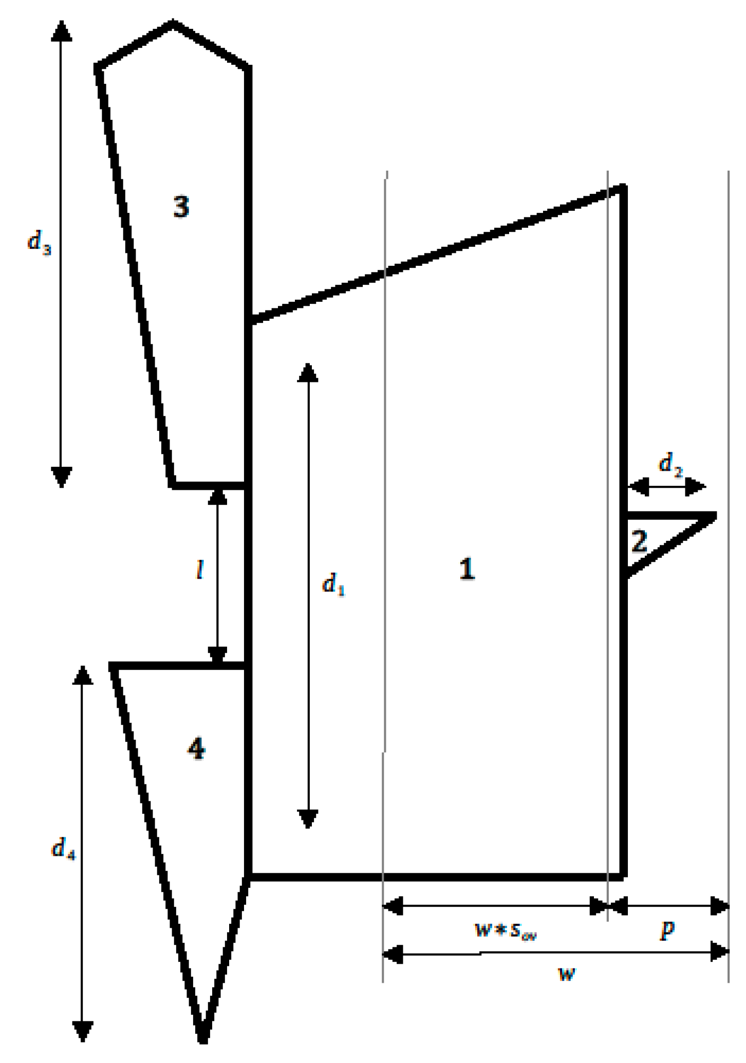
Then, if the UAV flies over a sub-region following its corresponding path (perpendicular to the sweep direction) and an adjacent sub-region (with the same path direction or another) fits in , then the second sub-region can be merged into the first one. For example, in Figure 5, if the UAV is flying over sub-region 1 following its path direction, , it can be appreciated that sub-region 2 is already being covered, despite having another flight direction, .
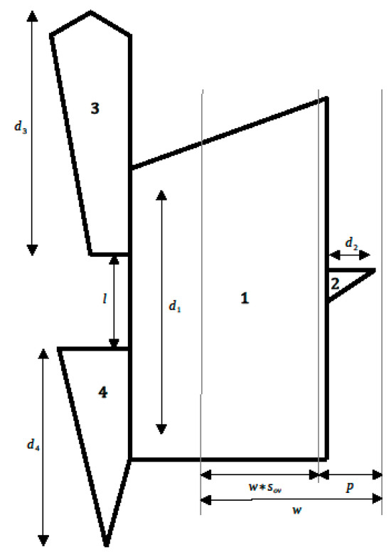
Figure 5.
Example of sub-regions to explain the second criteria. 1 and 2, and 1 and 3 can be merged. 4 can be merged as long as is less than the turning radio of the UAV.
On the other hand, the algorithm analyzes if two adjacent sub-polygons have the same flight direction, and if they do, then they are merged. In the event that two sub-regions were merged according to this criterion (see sub-regions 1 and 3 in Figure 5) and there is a third one with the same flight direction as the previous two (see sub-region 4 in Figure 5), adjacent to one of them and collinear but separated a distance from the other, then this third sub-region can only be merged with the other two when is shorter than the distance that the UAV needs to complete a 180-degree turn following the BF pattern of scanning. Realize that if the turning distance is considered approximately zero, as in rotatory-wing UAVs is usually done, then these sub-regions would always remain separated. For the benchmarking, due to a lack of data, was taken as a constant equal to 75 m for all the UAV models.
This merged criterion generates multiple combinations of sub-polygons. Thus, when the process is finished, the minimum sum of widths must be applied one second time, obtaining the final widths of each sub-polygon and their corresponding perpendicular path direction.
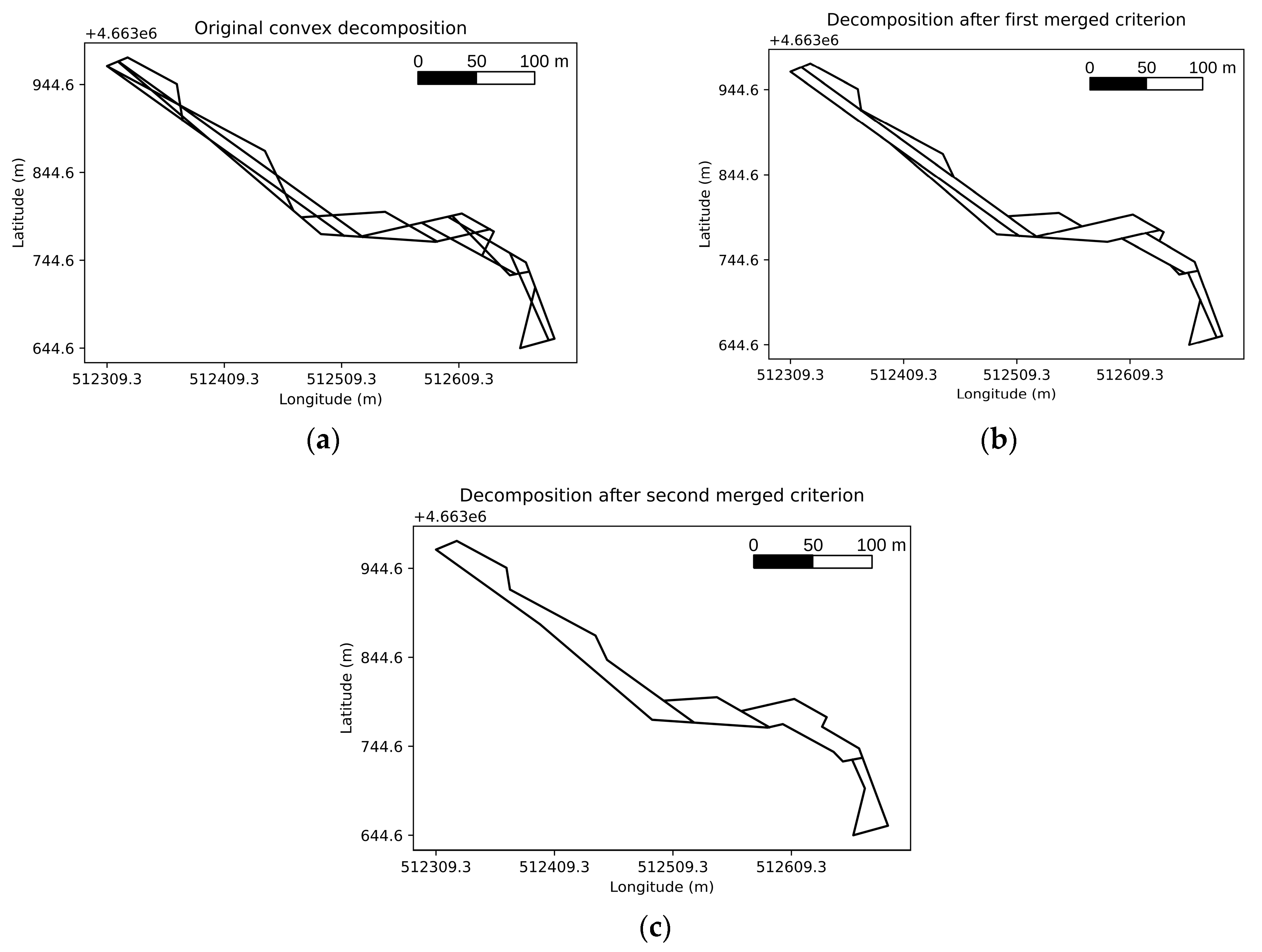
In Figure 6, it is illustrated how convex sub-polygons are merged in the first stage and the second stage, starting from the original convex decomposition. The number of sub-polygons has been reduced from 32 to 11 in the first step and from 11 to 4 in the second one for the Sony Alpha 7R IV sensor with the characteristics of Table 1 and Table 2.
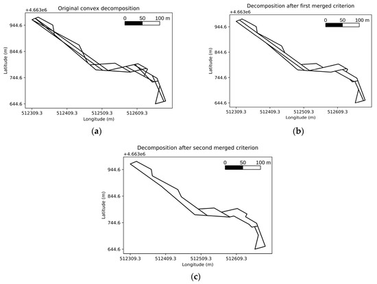
Figure 6.
Example of how both the first merged algorithm (b) and the second improved one for fixed-wing UAVs and long areas (c) work from the convex original partition (a).
Once the final sub-polygons are obtained with their corresponding main path directions, it is necessary to know how many sweeps are required to cover each sub-region completely, applying a Boustrophedon algorithm. This is calculated according to:
Making ⌈ ⌉ the ceiling function that returns the smallest integer greater than or equal to the input element, is the maximum value of the sub-polygon taking as coordinate system the sweep direction (abscissa axis) and the path direction (ordinate axis), is the minimum value of the sub-polygon taking as coordinate system the sweep direction (abscissa axis) and the path direction (ordinate axis), is the side overlap of the camera sensor expressed in per-unit, and is the HFOV of the camera sensor.
Finally, in order to obtain the sequence in which all the intra- and inter-sub-regions must be visited, the centroid of each sub-region is calculated, converting the problem into a TSP and solving it using a PSO algorithm, considering the aerodrome as the first and last point to be visited.
3. Results
In this section, the benchmarking of the UAVs and cameras is carried out. For this purpose, simulations were carried out according to the data in Table 2 and Table 3, applying the algorithm explained in the previous section.
The number of photos, the number of 180-degree turns created by the BF pattern, and the ideal distance traveled without considering the UAV and tidal restrictions can only vary depending on the camera model and its properties. In Table 4, they are summarized for each sensor. The traveled distance was calculated as the sum of the intra-region path planning (the CPP problem) plus the TSP route starting and ending in the aerodrome.
Table 4.
Number of photos, number of BF turns, and the ideal distance traveled according to each camera model without taking into account UAV and tidal restrictions.
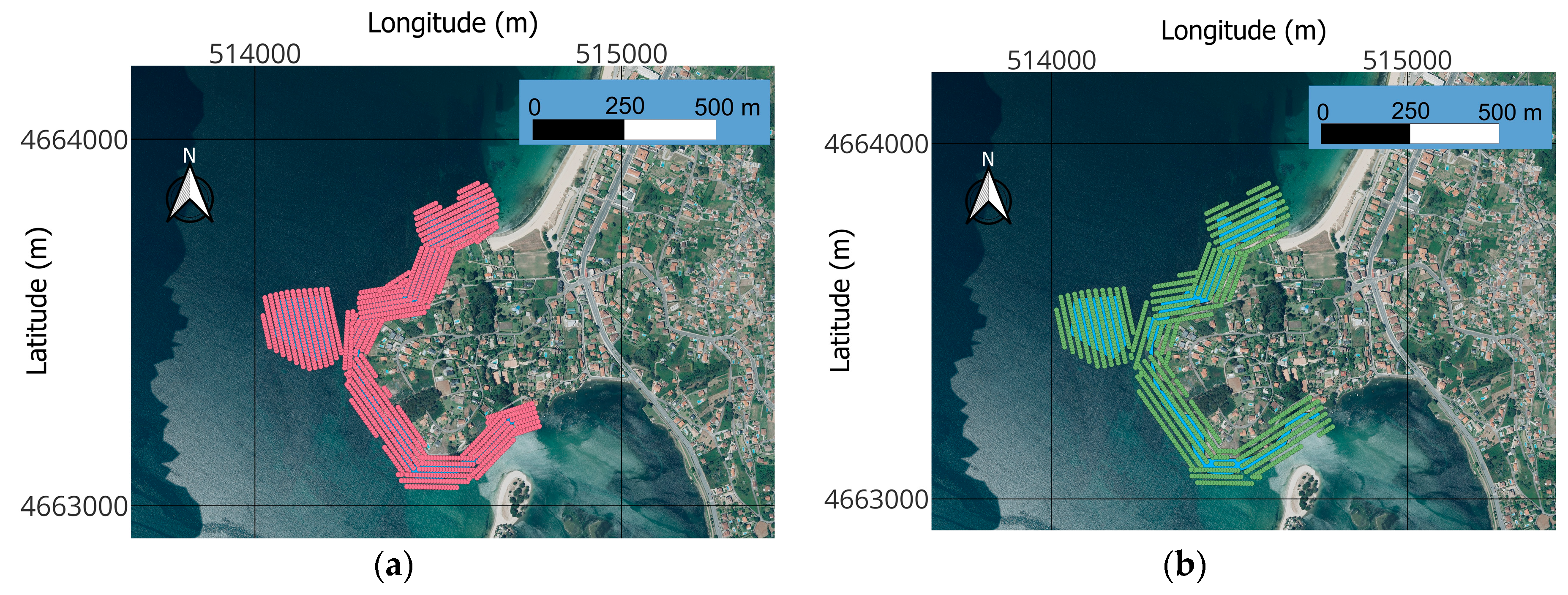
Table 4 shows the importance of choosing a suitable sensor, as the traveled distance may vary significantly. When a camera has a wider HFOV, the number of scans needed to cover an area is reduced and fewer turns are needed; consequently, the traveled distance will decrease. On the other hand, when a camera has a broader VFOV, it affects the number of photos, as the shooting frequency can be reduced. In Figure 7, two regions are covered by the Sony RX1RII, the Imperx T9040, and the PhaseOne iXM-100, and the points where photos must be taken are marked. It can be appreciated as the Sony RX1RII, with the narrowest HFOV, presents the closest points in the sweep direction, which means that the UAV will need more turns to complete the regions. Both the Sony RX1RII and the Imperx T9040 have a reduced VFOV; therefore, the shooting frequency is higher, and pictures must be closer in the path direction. Finally, the PhaseOne iXM-100 offers the best VFOV and HFOV, consequently reducing the number of necessary turns and photos.

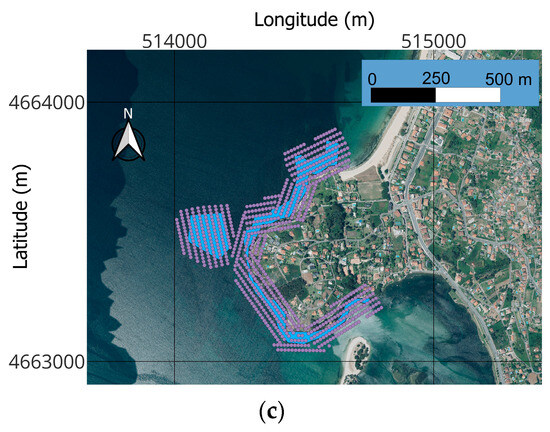
Figure 7.
Comparison between the Sony RX1RII (a), Imperx T9040 (b) and PhaseOne iXM-100 (c) attending to their HFOV and VFOV. Each point shows the position where each photo must be taken. (WGS84/UTM 29N).
If only the choice of the camera sensor were to be considered, the best option would be the PhaseOne iXM-100. However, the problem cannot be decoupled, and UAV properties and compatibility must also be analyzed.
In Table 5, the two-hour tidal interval and UAV properties from Table 3 were applied to obtain the number of necessary working days to cover all the regions, the number of battery changes (guaranteeing at least a 20% battery until the landing), the operational flight time and distance (without considering the first take-off and the last landing of each day as they do not compute in the two-hour window), and the total flight time and distance.
Table 5.
Main results obtained from the combination of each UAV with its compatible cameras.
The flight time is approximated, simplifying the problem as if UAVs could fly all the time at their cruise speed, from take-off to landing, plus 10 min of extra time in case of changing their batteries and flying again during the same day.
After simulating all the cases, and although there are several combinations that allow to complete all the tasks in two days, two options stand out from the rest: the Delair DT26 Open Payload with the PhaseOne iXM-100 camera and the Heliplane LRS 340 PRO with the Sony Alpha 7R IV.
The first one presents the best sensor, which allows for minimizing the number of turns, pictures, and path distance. On the other side, the LRS 340 PRO is the UAV with the best performance, and, even though it cannot incorporate the best camera, it can finish the work in minimum time as it reaches the highest cruise speed. In Table 6, these results are summarized and the difference, in percentage, between the Delair and Heliplane is calculated.
Table 6.
The two outstanding options for covering all the regions.
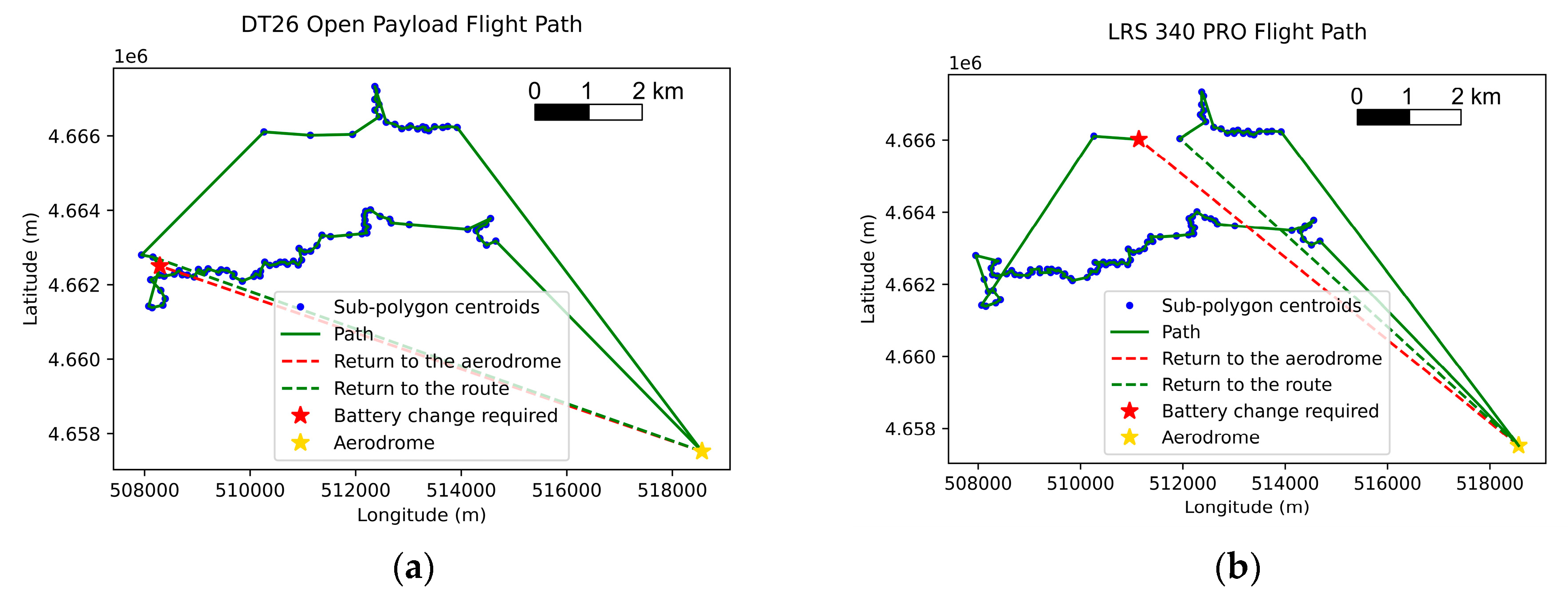
Finally, the inter sub-region flight path of both cases is shown in Figure 8.
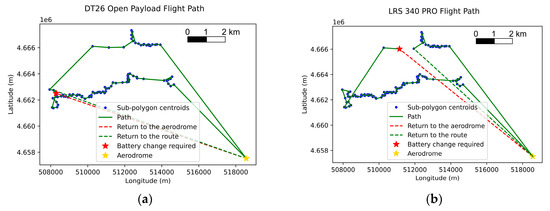
Figure 8.
Flight paths following clockwise direction. Delair DT26 Open Payload with PhaseOne iXM-100 camera (a) and Heliplane LRS 340 PRO with Sony Alpha 7R IV (b). (WGS84/UTM 29N).
4. Discussion
Traditional methods for data acquisition in intertidal regions are limited by low tide intervals, hard-to-reach areas, and highly concentrated sampling, which does not allow for observation of large-area patterns. Some studies were carried out with satellite imagery or manned aerial platforms, but the resolution was too low. Recently, rotatory-wing UAVs were also employed. However, either study areas were small, or GSD values were high. In this work, it was proposed to use small fixed-wing electric UAVs with very high-resolution cameras for goose barnacle and mussel seed data collection and photogrammetry tasks along the Galician coastline. These aircraft can fly for hours, covering long distances and reaching higher speeds than the rotatory-wing UAVs, which makes them more suitable for these tasks.
In order to choose the best combination among some commercial alternatives, a real scenario consisting of 15 isolated regions that must be completely covered was created. To solve this problem, an algorithm based on an Exact Cellular Decomposition Coverage Path Planning (CPP) for intra-region coverage and a Traveling Salesman Problem (TSP) to obtain the inter-region path was proposed. This algorithm was intended specifically for enhancing the cellular merging process and reducing the number of sub-regions for fixed-wing UAVs that must cover long areas with sharp corners. The number of sub-regions is directly related to the number of turns to cover an area and, therefore, to the flight efficiency. Results allow us to compare the number of photos, turns, working days, and battery changes needed for each combination, as well as the total flight distance and time.
Although the CPP and the TSP already present high complexity and computational cost separately, they should not be decoupled, which further complicates the problem by having to consider the entry and exit points of the UAV in each region [30,31,32]. However, benchmarking was enough to solve them separately. This is because we were looking for a standardized and realistic method to compare all the cases instead of the global optimal result, and we need to speed up the calculation as there are several combinations that must be simulated.
This benchmarking shows that, although there are several alternatives to complete the job in two days with a single battery change, there are two options that stand out from the rest: the Delair DT26 Open Payload with the PhaseOne iXM-100 camera and the Heliplane LRS 340 PRO with the Sony Alpha 7R IV. The Delair can carry the best sensor, which means that it can finish the route with the minimum number of pictures, turns and flight distance (8.4%, 15.2% and 5.9% less than Heliplane, respectively). However, the Heliplane has the highest cruise speed, which means that it can finish the route in a 19.8% less time than the DT26 Open Payload.
Solutions were accurate enough, converting this algorithm into a useful tool not only for comparing fixed-wing UAVs and sensor performances, helping to select the best combination, but also to obtain a preliminary inspection plan, especially in missions carried out in long areas such as search and rescue, surveillance, monitoring, or photogrammetry. Besides, if the turning distance is taken approximately as zero, then the parameter will never satisfy the conditions of the second polygon merged stage, and the algorithm may also be profitable for rotatory-wing UAVs (see Section 2.4).
Notice that to obtain more realistic results in flight time and distance, BF turns must be considered [26,27], as fixed-wing UAVs present maneuver constraints and it is necessary to fly out of the region of interest to complete them or even reduce the speed during the maneuver, increasing time, distance, and energy consumption. Consequently, it is very likely that these constraints affect the Heliplane more than the Delair because of the greater number of turns in its trajectory. Therefore, differences in flight time may be reduced, and then the Delair DT26 Open Payload incorporating the PhaseOne iXM-100 should be the best choice, although further research must be carried out.
Another field of research is the consideration of the VTOL (Vertical Take-Off and Landing) capacity of some fixed-wing UAVs. In this article, it was not considered to maintain a standard scenario during the benchmarking, with the same take-off and landing point for all the cases, but this could be of great interest when calculating the optimal path or battery change points.
5. Conclusions
The use of fixed-wing UAVs instead of rotatory-wing UAVs for photogrammetry and data acquisition to monitor and control mussel seed and goose barnacle populations on the Galician coast is proposed, as it is intended to guarantee a low GSD and intertidal regions are very large. Using a CPP algorithm enhanced for fixed-wing UAVs and long areas with sharp corners and a TSP algorithm, some commercial fixed-wing electric UAVs with compatible very high-resolution cameras were simulated to benchmark them and choose the best combination.
After that, results show that the Delair DT26 Open Payload with the PhaseOne iXM-100 camera (minimum distance, number of photos and turns) and the Heliplane LRS 340 PRO incorporating the Sony Alpha 7R IV (minimum flight time) stand out from the rest.
In fact, the number of days required for the proposed inspection can increase significantly using other worse configurations considered in this work. This underscores the importance of conducting a thorough assessment before implementing a UAV-based intertidal monitoring system since a bad choice could have a significant negative impact, increasing personnel costs and working time. In this regard, benchmarking methodologies such as the one proposed in this work are necessary for a quantitative analysis of the performance of the various UAV and camera configurations available. This assessment methodology could also be applied to other applications of coverage path planning, such as search and rescue, surveillance, photogrammetry, or data acquisition of any other type. Even though it was initially designed for fixed-wing UAVs covering extensive areas with sharp corners, it may be suitable for rotary-wing UAVs and other scenarios with minor parameter adjustments.
More research, mainly implementing fixed-wing constraints, must be performed for refined results, although the first option is probably the most suitable because of the minimum number of BF turns. Further research can also be done to optimize the path planning system, as CPP and TSP problems were considered separate to simplify the problem and speed up the calculations, and the VTOL mode was not implemented. In addition, it would be interesting to compare this algorithm with other existing ones for analyzing its effectiveness in optimizing the task. Finally, in future work, real flight tests will be carried out to verify the obtained results.
Author Contributions
Conceptualization, G.F.-C., E.A., H.G.-J. and F.V.; methodology, G.F.-C. and E.A.; software, G.F.-C.; validation, G.F.-C.; formal analysis, G.F.-C. and E.A.; investigation, G.F.-C. and E.A.; resources, G.F.-C. and E.A.; data curation, G.F.-C. and E.A.; writing—original draft preparation, G.F.-C.; writing—review and editing, H.G.-J. and F.V.; visualization, G.F.-C.; supervision, H.G.-J. and F.V.; project administration, H.G.-J. and F.V.; funding acquisition, H.G.-J. All authors have read and agreed to the published version of the manuscript.
Funding
Authors would like to thank University of Vigo, CISUG, Xunta de Galicia, Gobierno de España, Agencia Estatal de Investigación and European Union—Next GenerationEU for the financial support given through the next grants: FPU21/01176. PID2021-125060OB-100. TED2021-129756B-C31. Complementary R&D Plan. Galician Marine Sciences Program. Funding for open access charge (University of Vigo/CISUG).
Data Availability Statement
The data used in this study are not publicly available due to the conditions of the ethics approval for the study. Contact the corresponding author for further information.
Acknowledgments
Authors would like to thank the Ecology and Zoology Group of the University of Vigo for the marine biological knowledge provided and the experience of working with them, and Eduardo Ríos-Otero by supporting us in marine UAV missions.
Conflicts of Interest
The authors declare no conflict of interest.
References
- Figueras, A. MYTILIDAE. Cultured Aquatic Species Information Programme. Available online: https://www.fao.org/fishery/en/culturedspecies/mytilus_galloprovincialis?lang=en (accessed on 2 August 2023).
- Figueiras, F.G.; Labarta, U.; Fernández Reiriz, M.J. Coastal Upwelling, Primary Production and Mussel Growth in the Rias Baixas of Galicia. Hydrobiologia 2002, 484, 121–131. [Google Scholar] [CrossRef]
- Pita, P.; Fernández-Márquez, D.; Antelo, M.; Macho, G.; Villasante, S. Socioecological Changes in Data-Poor S-Fisheries: A Hidden Shellfisheries Crisis in Galicia (NW Spain). Mar. Policy 2019, 101, 208–224. [Google Scholar] [CrossRef]
- Fraga-Corral, M.; Ronza, P.; Garcia-Oliveira, P.; Pereira, A.G.; Losada, A.P.; Prieto, M.A.; Quiroga, M.I.; Simal-Gandara, J. Aquaculture as a Circular Bio-Economy Model with Galicia as a Study Case: How to Transform Waste into Revalorized by-Products. Trends Food Sci. Technol. 2022, 119, 23–35. [Google Scholar] [CrossRef]
- Babarro, J.M.F.; Filgueira, R.; Padín, X.A.; Longa Portabales, M.A. A Novel Index of the Performance of Mytilus galloprovincialis to Improve Commercial Exploitation in Aquaculture. Front. Mar. Sci. 2020, 7, 719. [Google Scholar] [CrossRef]
- Brown, C. Seaglider Observations of Biogeochemical Variability in the Iberian Upwelling System. Ph.D. Thesis, University of East Anglia, Norwich, UK, 2013. [Google Scholar]
- Pérez-Camacho, A.; Labarta, U.; Vinseiro, V.; Fernández-Reiriz, M.J. Mussel Production Management: Raft Culture without Thinning-Out. Aquaculture 2013, 406–407, 172–179. [Google Scholar] [CrossRef]
- Sousa, A.; Jacinto, D.; Penteado, N.; Pereira, D.; Silva, T.; Castro, J.J.; Leandro, S.M.; Cruz, T. Temporal Variation of the Fishers’ Perception about the Stalked Barnacle (Pollicipes pollicipes) Fishery at the Berlengas Nature Reserve (Portugal). Reg. Stud. Mar. Sci. 2020, 38, 101378. [Google Scholar] [CrossRef]
- Gomes, I.; Peteiro, L.; Bueno-Pardo, J.; Albuquerque, R.; Pérez-Jorge, S.; Oliveira, E.R.; Alves, F.L.; Queiroga, H. What’s a Picture Really Worth? On the Use of Drone Aerial Imagery to Estimate Intertidal Rocky Shore Mussel Demographic Parameters. Estuar. Coast. Shelf Sci. 2018, 213, 185–198. [Google Scholar] [CrossRef]
- Molares, J.; Freire, J. Development and Perspectives for Community-Based Management of the Goose Barnacle (Pollicipes pollicipes) Fisheries in Galicia (NW Spain). Fish Res. 2003, 65, 485–492. [Google Scholar] [CrossRef]
- de Galicia, P. Plans de Percebe: Zonas de Reserva Para Semente de Mexillón. Available online: https://www.pescadegalicia.gal/gl/zonasreservamexilla_zonasexclusivaspercebe (accessed on 9 August 2023).
- Fiori, L.; Doshi, A.; Martinez, E.; Orams, M.B.; Bollard-Breen, B. The Use of Unmanned Aerial Systems in Marine Mammal Research. Remote Sens. 2017, 9, 543. [Google Scholar] [CrossRef]
- Reineman, B.D.; Lenain, L.; Melville, W.K. The Use of Ship-Launched Fixed-Wing UAVs for Measuring the Marine Atmospheric Boundary Layer and Ocean Surface Processes. J. Atmos. Ocean. Technol. 2016, 33, 2029–2052. [Google Scholar] [CrossRef]
- Seymour, A.C.; Ridge, J.T.; Rodriguez, A.B.; Newton, E.; Dale, J.; Johnston, D.W. Deploying Fixed Wing Unoccupied Aerial Systems (UAS) for Coastal Morphology Assessment and Management. J. Coast. Res. 2018, 34, 704. [Google Scholar] [CrossRef]
- Giles, A.B.; Ren, K.; Davies, J.E.; Abrego, D.; Kelaher, B. Combining Drones and Deep Learning to Automate Coral Reef Assessment with RGB Imagery. Remote Sens. 2023, 15, 2238. [Google Scholar] [CrossRef]
- Colefax, A.P.; Butcher, P.A.; Pagendam, D.E.; Kelaher, B.P. Reliability of Marine Faunal Detections in Drone-Based Monitoring. Ocean Coast. Manag. 2019, 174, 108–115. [Google Scholar] [CrossRef]
- Ventura, D.; Bonifazi, A.; Gravina, M.F.; Belluscio, A.; Ardizzone, G. Mapping and Classification of Ecologically Sensitive Marine Habitats Using Unmanned Aerial Vehicle (UAV) Imagery and Object-Based Image Analysis (OBIA). Remote Sens. 2018, 10, 1331. [Google Scholar] [CrossRef]
- Ventura, D.; Grosso, L.; Pensa, D.; Casoli, E.; Mancini, G.; Valente, T.; Scardi, M.; Rakaj, A. Coastal Benthic Habitat Mapping and Monitoring by Integrating Aerial and Water Surface Low-Cost Drones. Front. Mar. Sci. 2023, 9, 1096594. [Google Scholar] [CrossRef]
- Brunier, G.; Oiry, S.; Lachaussée, N.; Barillé, L.; Le Fouest, V.; Méléder, V. A Machine-Learning Approach to Intertidal Mudflat Mapping Combining Multispectral Reflectance and Geomorphology from UAV-Based Monitoring. Remote Sens. 2022, 14, 5857. [Google Scholar] [CrossRef]
- Barbosa, R.V.; Jaud, M.; Bacher, C.; Kerjean, Y.; Jean, F.; Ammann, J.; Thomas, Y. High-Resolution Drone Images Show That the Distribution of Mussels Depends on Microhabitat Features of Intertidal Rocky Shores. Remote Sens. 2022, 14, 5441. [Google Scholar] [CrossRef]
- Roca, M.; Dunbar, M.B.; Román, A.; Caballero, I.; Zoffoli, M.L.; Gernez, P.; Navarro, G. Monitoring the Marine Invasive Alien Species Rugulopteryx okamurae Using Unmanned Aerial Vehicles and Satellites. Front. Mar. Sci. 2022, 9, 1004012. [Google Scholar] [CrossRef]
- Román, A.; Tovar-Sánchez, A.; Olivé, I.; Navarro, G. Using a UAV-Mounted Multispectral Camera for the Monitoring of Marine Macrophytes. Front. Mar. Sci. 2021, 8, 722698. [Google Scholar] [CrossRef]
- Kellaris, A.; Gil, A.; Faria, J.; Amaral, R.; Moreu-Badia, I.; Neto, A.; Yesson, C. Using Low-cost Drones to Monitor Heterogeneous Submerged Seaweed Habitats: A Case Study in the Azores. Aquat. Conserv. Mar. Freshw. Ecosyst. 2019, 29, 1909–1922. [Google Scholar] [CrossRef]
- Instituto Geográfico Nacional. Longitud de La Línea de Costa Española Por Provincias. Available online: https://www.ign.es/web/ane-datos-geograficos/-/datos-geograficos/datosGenerales?tipoBusqueda=longCosta (accessed on 9 August 2023).
- Cabreira, T.; Brisolara, L.; Ferreira, P.R., Jr. Survey on Coverage Path Planning with Unmanned Aerial Vehicles. Drones 2019, 3, 4. [Google Scholar] [CrossRef]
- Yuan, J.; Liu, Z.; Lian, Y.; Chen, L.; An, Q.; Wang, L.; Ma, B. Global Optimization of UAV Area Coverage Path Planning Based on Good Point Set and Genetic Algorithm. Aerospace 2022, 9, 86. [Google Scholar] [CrossRef]
- Huang, J.; Fu, W.; Luo, S.; Wang, C.; Zhang, B.; Bai, Y. A Practical Interlacing-Based Coverage Path Planning Method for Fixed-Wing UAV Photogrammetry in Convex Polygon Regions. Aerospace 2022, 9, 521. [Google Scholar] [CrossRef]
- DELTAQUAD. Explore the DeltaQuad Pro VTOL UAV. Available online: https://www.deltaquad.com/?utm_term=deltaquad&utm_campaign=EN%20-%20Branded&utm_source=Google&utm_medium=cpc&hsa_acc=1674375646&hsa_cam=1983332835&hsa_grp=73742855449&hsa_ad=651564717761&hsa_src=g&hsa_tgt=kwd-665960707668&hsa_kw=deltaquad&hsa_mt=p&hsa_net=adwords&hsa_ver=3&gad=1&gclid=CjwKCAjw8symBhAqEiwAaTA__L4_UNNARYJD0d-vf7I4LkauM4jdSk89t2MIiBQqdxaaTkqRIeVkfhoCg7cQAvD_BwE (accessed on 9 August 2023).
- Delair DT46. Available online: https://delair.aero/delair-commercial-drones/dt46-long-range-made-easy/ (accessed on 9 August 2023).
- Xie, J.; Carrillo, L.R.G.; Jin, L. An Integrated Traveling Salesman and Coverage Path Planning Problem for Unmanned Aircraft Systems. IEEE Control Syst. Lett. 2019, 3, 67–72. [Google Scholar] [CrossRef]
- Khanam, Z.; McDonald-Maier, K.; Ehsan, S. Near-Optimal Coverage Path Planning of Distributed Regions for Aerial Robots with Energy Constraint. In Proceedings of the 2021 International Conference on Unmanned Aircraft Systems (ICUAS), Athens, Greece, 15 June 2021; pp. 1659–1664. [Google Scholar]
- Xie, J.; Chen, J. Multiregional Coverage Path Planning for Multiple Energy Constrained UAVs. IEEE Trans. Intell. Transp. Syst. 2022, 23, 17366–17381. [Google Scholar] [CrossRef]
- Nielsen, L.D.; Sung, I.; Nielsen, P. Convex Decomposition for a Coverage Path Planning for Autonomous Vehicles: Interior Extension of Edges. Sensors 2019, 19, 4165. [Google Scholar] [CrossRef]
- Gong, Y.; Chen, K.; Niu, T.; Liu, Y. Grid-Based Coverage Path Planning with NFZ Avoidance for UAV Using Parallel Self-Adaptive Ant Colony Optimization Algorithm in Cloud IoT. J. Cloud Comput. 2022, 11, 29. [Google Scholar] [CrossRef]
- Galceran, E.; Carreras, M. A Survey on Coverage Path Planning for Robotics. Robot. Auton. Syst. 2013, 61, 1258–1276. [Google Scholar] [CrossRef]
- Tang, G.; Tang, C.; Zhou, H.; Claramunt, C.; Men, S. R-DFS: A Coverage Path Planning Approach Based on Region Optimal Decomposition. Remote Sens. 2021, 13, 1525. [Google Scholar] [CrossRef]
- Xu, A.; Viriyasuthee, C.; Rekleitis, I. Efficient Complete Coverage of a Known Arbitrary Environment with Applications to Aerial Operations. Auton. Robot. 2014, 36, 365–381. [Google Scholar] [CrossRef]
- Xu, A.; Viriyasuthee, C.; Rekleitis, I. Optimal Complete Terrain Coverage Using an Unmanned Aerial Vehicle. In Proceedings of the 2011 IEEE International Conference on Robotics and Automation, Shanghai, China, 9–13 May 2011; pp. 2513–2519. [Google Scholar]
- Papaioannou, S.; Kolios, P.; Theocharides, T.; Panayiotou, C.G.; Polycarpou, M.M. Integrated Guidance and Gimbal Control for Coverage Planning With Visibility Constraints. IEEE Trans. Aerosp. Electron. Syst. 2022, 59, 1276–1291. [Google Scholar] [CrossRef]
- Choset, H. Coverage for Robotics—A Survey of Recent Results. Ann. Math. Artif. Intell. 2001, 31, 113–126. [Google Scholar] [CrossRef]
- Jimenez, P.A.; Shirinzadeh, B.; Nicholson, A. Gursel Alici Optimal Area Covering Using Genetic Algorithms. In Proceedings of the 2007 IEEE/ASME International Conference on Advanced Intelligent Mechatronics, Zurich, Switzerland, 4–7 September 2007; pp. 1–5. [Google Scholar]
- Mannadiar, R.; Rekleitis, I. Optimal Coverage of a Known Arbitrary Environment. In Proceedings of the 2010 IEEE International Conference on Robotics and Automation, Anchorage, Alaska, 3–8 May 2010; pp. 5525–5530. [Google Scholar]
- Li, Y.; Chen, H.; Joo Er, M.; Wang, X. Coverage Path Planning for UAVs Based on Enhanced Exact Cellular Decomposition Method. Mechatronics 2011, 21, 876–885. [Google Scholar] [CrossRef]
- Huang, W.H. Optimal Line-Sweep-Based Decompositions for Coverage Algorithms. In Proceedings of the 2001 ICRA. IEEE International Conference on Robotics and Automation (Cat. No.01CH37164), Seoul, Republic of Korea, 21–26 May 2001; pp. 27–32. [Google Scholar]
- Jiao, Y.-S.; Wang, X.-M.; Chen, H.; Yan, L. Research on the Coverage Path Planning of UAVs for Polygon Areas. In Proceedings of the 2010 5th IEEE Conference on Industrial Electronics and Applications, Taichung, Taiwan, 15–17 June 2010; pp. 1467–1472. [Google Scholar]
- Akshya, J.; Priyadarsini, P.L.K. Area Partitioning by Intelligent UAVs for Effective Path Planning Using Evolutionary Algorithms. In Proceedings of the 2021 International Conference on Computer Communication and Informatics (ICCCI), Coimbatore, India, 27 January 2021; pp. 1–6. [Google Scholar]
- Phung, M.D.; Quach, C.H.; Dinh, T.H.; Ha, Q. Enhanced Discrete Particle Swarm Optimization Path Planning for UAV Vision-Based Surface Inspection. Autom. Constr. 2017, 81, 25–33. [Google Scholar] [CrossRef]
- Bolourian, N.; Hammad, A. LiDAR-Equipped UAV Path Planning Considering Potential Locations of Defects for Bridge Inspection. Autom. Constr. 2020, 117, 103250. [Google Scholar] [CrossRef]
- Lim, K.K.; Ong, Y.-S.; Lim, M.H.; Chen, X.; Agarwal, A. Hybrid Ant Colony Algorithms for Path Planning in Sparse Graphs. Soft Comput. 2008, 12, 981–994. [Google Scholar] [CrossRef]
- Bera, A.; Misra, S.; Chatterjee, C.; Mao, S. CEDAN: Cost-Effective Data Aggregation for UAV-Enabled IoT Networks. IEEE Trans. Mob. Comput. 2022, 22, 5053–5063. [Google Scholar] [CrossRef]
- Ministerio Para la Transición Ecológica y el Reto Demográfico Criterios Para el Vuelo de Drones en ZEPA Marinas de Competencia Estatal. Available online: https://www.miteco.gob.es/es/biodiversidad/temas/biodiversidad-marina/espacios-marinos-protegidos/red-natura-2000-ambito-marino/bm_emprot_rednat2000_marino_vuelo_drones.html (accessed on 6 September 2023).
- Sony E-MOUNT FE 50mm F1.8. Available online: https://www.sony.co.uk/electronics/camera-lenses/sel50f18f (accessed on 11 August 2023).
- Sony A7R IV 35mm Full-Frame Camera with 61.0MP. Full Specifications & Features-7RM4. Available online: https://www.sony.co.uk/electronics/interchangeable-lens-cameras/ilce-7rm4/specifications (accessed on 11 August 2023).
- Sony RX1R II Professional Compact Camera with 35 mm Sensor. Available online: https://www.sony.com/za/electronics/cyber-shot-compact-cameras/dsc-rx1rm2#product_details_default (accessed on 11 August 2023).
- IMPERX T9040. Available online: https://www.imperx.com/ccd-cameras/t9040/ (accessed on 11 August 2023).
- Mastelic, T.; Lorincz, J.; Ivandic, I.; Boban, M. Aerial Imagery Based on Commercial Flights as Remote Sensing Platform. Sensors 2020, 20, 1658. [Google Scholar] [CrossRef]
- IXM-100|IXM-50 a Revolution in UAV and Drone Cameras. Available online: https://geospatial.phaseone.com/cameras/ixm-100/ (accessed on 11 August 2023).
- Contreras-de-Villar, F.; García, F.J.; Muñoz-Perez, J.J.; Contreras-de-Villar, A.; Ruiz-Ortiz, V.; Lopez, P.; Garcia-López, S.; Jigena, B. Beach Leveling Using a Remotely Piloted Aircraft System (RPAS): Problems and Solutions. J. Mar. Sci. Eng. 2020, 9, 19. [Google Scholar] [CrossRef]
- de Lima, R.S.; Lang, M.; Burnside, N.G.; Peciña, M.V.; Arumäe, T.; Laarmann, D.; Ward, R.D.; Vain, A.; Sepp, K. An Evaluation of the Effects of UAS Flight Parameters on Digital Aerial Photogrammetry Processing and Dense-Cloud Production Quality in a Scots Pine Forest. Remote Sens. 2021, 13, 1121. [Google Scholar] [CrossRef]
- DT26 Open Payload. Available online: https://delair.aero/delair-commercial-drones/dt26-open-payload/#package (accessed on 14 August 2023).
- DeltaQuad Pro #MAP Smart UAV Technology for Mapping & Surveying. Available online: https://www.deltaquad.com/vtol-drones/map/#specifications (accessed on 14 August 2023).
- TRINITY F90+ CAMERAS. Available online: https://quantum-systems.com/wp-content/uploads/2023/01/QS_Trinity_Overview_Cameras_V01_220711.pdf (accessed on 14 August 2023).
- TRINITY F90+ EVTOL. Fixed-Wing. Mapping UAS. Available online: https://quantum-systems.com/wp-content/uploads/2023/01/QS_TrinityF90_Overview_220912.pdf (accessed on 14 August 2023).
- HELIPLANE LRS. Long Endurance VTOL Drone. Available online: https://www.dronevolt.com/en/expert-solutions/heliplane/#features (accessed on 14 August 2023).
- C-ASTRAL Aerospace. Bramor PpX Survey Grade UAS. Available online: https://www.c-astral.com/en/unmanned-systems/bramor-ppx (accessed on 16 August 2023).
- AeroVironment. PUMA LE. Available online: https://www.avinc.com/uas/puma-le (accessed on 16 August 2023).
- QGIS.org QGIS Geographic Information System 2023. Available online: https://www.qgis.org/en/site/ (accessed on 16 August 2023).


Disclaimer/Publisher’s Note: The statements, opinions and data contained in all publications are solely those of the individual author(s) and contributor(s) and not of MDPI and/or the editor(s). MDPI and/or the editor(s) disclaim responsibility for any injury to people or property resulting from any ideas, methods, instructions or products referred to in the content. |
© 2023 by the authors. Licensee MDPI, Basel, Switzerland. This article is an open access article distributed under the terms and conditions of the Creative Commons Attribution (CC BY) license (https://creativecommons.org/licenses/by/4.0/).