Article

On the Fidelity of RANS-Based Turbulence Models in Modeling the Laminar Separation Bubble and Ice-Induced Separation Bubble at Low Reynolds Numbers on Unmanned Aerial Vehicle Airfoil

by
Manaf Muhammed
* and
Muhammad Shakeel Virk
Arctic Technology & Icing Research Group, UiT—The Arctic University of Norway, 8514 Narvik, Norway
*
Author to whom correspondence should be addressed.
Drones 2024, 8(4), 148; https://doi.org/10.3390/drones8040148
Submission received: 15 February 2024 / Revised: 22 March 2024 / Accepted: 22 March 2024 / Published: 9 April 2024

Abstract

:
The operational regime of Unmanned Aerial Vehicles (UAVs) is distinguished by the dominance of laminar flow and the flow field is characterized by the appearance of Laminar Separation Bubbles (LSBs). Ice accretion on the leading side of the airfoil leads to the formation of an Ice-induced Separation Bubble (ISB). These separation bubbles have a considerable influence on the pressure, heat flux, and shear stress distribution on the surface of airfoils and can affect the prediction of aerodynamic coefficients. Therefore, it is necessary to capture these separation bubbles in the numerical simulations. Previous studies have shown that these bubbles can be modeled successfully using the Large Eddy Simulation (LES) and Direct Numerical Simulation (DNS) but are computationally costly. Also, for numerical modeling of ice accretion, the flow field needs to be recomputed at specific intervals, thus making LES and DNS unsuitable for ice accretion simulations. Thus, it is necessary to come up with a Reynolds-Averaged Navier–Stokes (RANS) equation-based model that can predict the LSBs and ISBs as accurately as possible. Numerical studies were performed to assess the fidelity of various RANS turbulence models in predicting LSBs and ISBs. The findings are compared with the experimental and LES data available in the literature. The structure of these bubbles is only studied from a pressure coefficient perspective, so an attempt is made in these studies to explain it using the skin friction coefficient distribution. The results indicate the importance of the use of transition-based models when dealing with low-Reynolds-number applications that involve LSB. ISB can be predicted by conventional RANS models but are subjected to high levels of uncertainty. Possible recommendations were made with respect to turbulence models when dealing with flows involving LSBs and ISBs, especially for ice accretion simulations.

1. Introduction

Turbulent flow often dominates the operational regime of manned aircraft traveling at high Reynolds numbers ( R e ) of O ( 10 6 ) and higher. Under such circumstances, viscous force causes flow separation to be delayed. The flow field around a UAV flying at a low R e of O ( 10 5 ) or lower is primarily of laminar nature and is sensitive to even minor pressure differences. Previous studies have demonstrated the formation of LSBs at these Reynolds numbers [1]. An extensive review of the flows involving LSBs was performed by Tani [2] in 1964. Ice accumulation on the leading side of an airfoil can lead to the creation of an ISB. Bragg et al. [3] primarily studied the production of such bubbles and the related deterioration of aerodynamic performance. Most of his studies are based on manned aircraft Ice accretion with Reynolds numbers in the order of 10 6 and the observations were not verified for low Reynolds number ranges. Manaf [4,5] conducted a comprehensive review of the impact of ice accumulation on UAVs and their aerodynamics in 2022–2023. The appearance of LSBs and ISBs can affect the aerodynamic coefficients by influencing the pressure and shear stress distributions considerably [6]. Further, it can also affect the heat flux distribution of the airfoil. The numerical ice accretion solvers demand accurate modeling of the flow field around the airfoil because heat flux and shear stress are the two main parameters that determine the water transport and ice accretion phenomena on the surface of the airfoil [7]. The capability of DNS and LES in predicting LSBs and ISBs can be found in the literature [1,8]. Implementing DNS/LES models for ice accretion simulations is expensive and is not feasible for multi-shot simulations (an iterative process to predict ice accretion with recalculation of the flow field at specific intervals). Loth [9] estimated the computational cost of various numerical approaches on the basis of the Reynolds number and found values of R e L 2.3 ,   R e L 1.8 , a n d   R e L 0.2 for DNS, LES, and RANS simulations, respectively. Therefore, using DNS and LES for an ice accretion prediction numerical solver is not feasible, especially for multi-shot icing simulations, which demand a flow field recalculation at every shot. Thus, it is necessary to come up with an effective RANS-based model that can predict LSBs and ISBs as accurately as possible. This study attempts to compare nine distinct RANS-based turbulence models to assess their capability in predicting LSBs and ISBs on Rg-15 airfoil at low values of R e . The effectiveness of existing turbulence models based on RANS equations in predicting LSBs and ISBs is studied by comparing their predictions with data available in the literature. Oo et al. [6] performed experimental and LES studies on LSBs and ISBs in 2020 around an Rg-15 airfoil at R e = O 10 5 , and the separation and reattachment locations were identified. Further, an attempt was also made to understand the dynamics and structure of these bubbles from the perspective of the skin friction coefficient, which was studied earlier but only from the perspective of pressure coefficients. A brief literature review of the current wisdom about LSBs and ISBs is presented below.

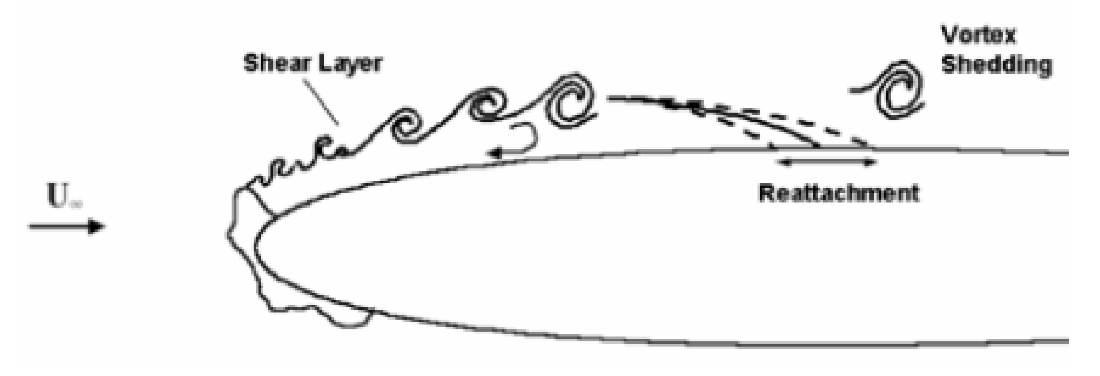
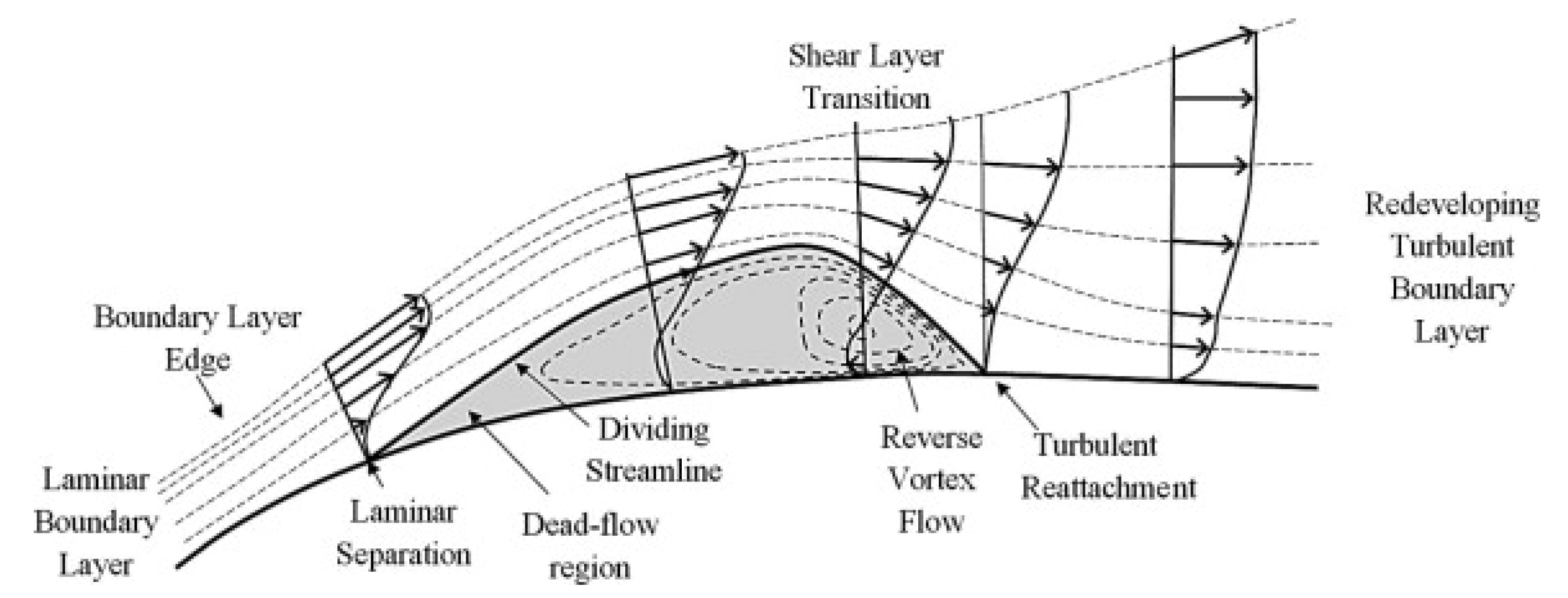
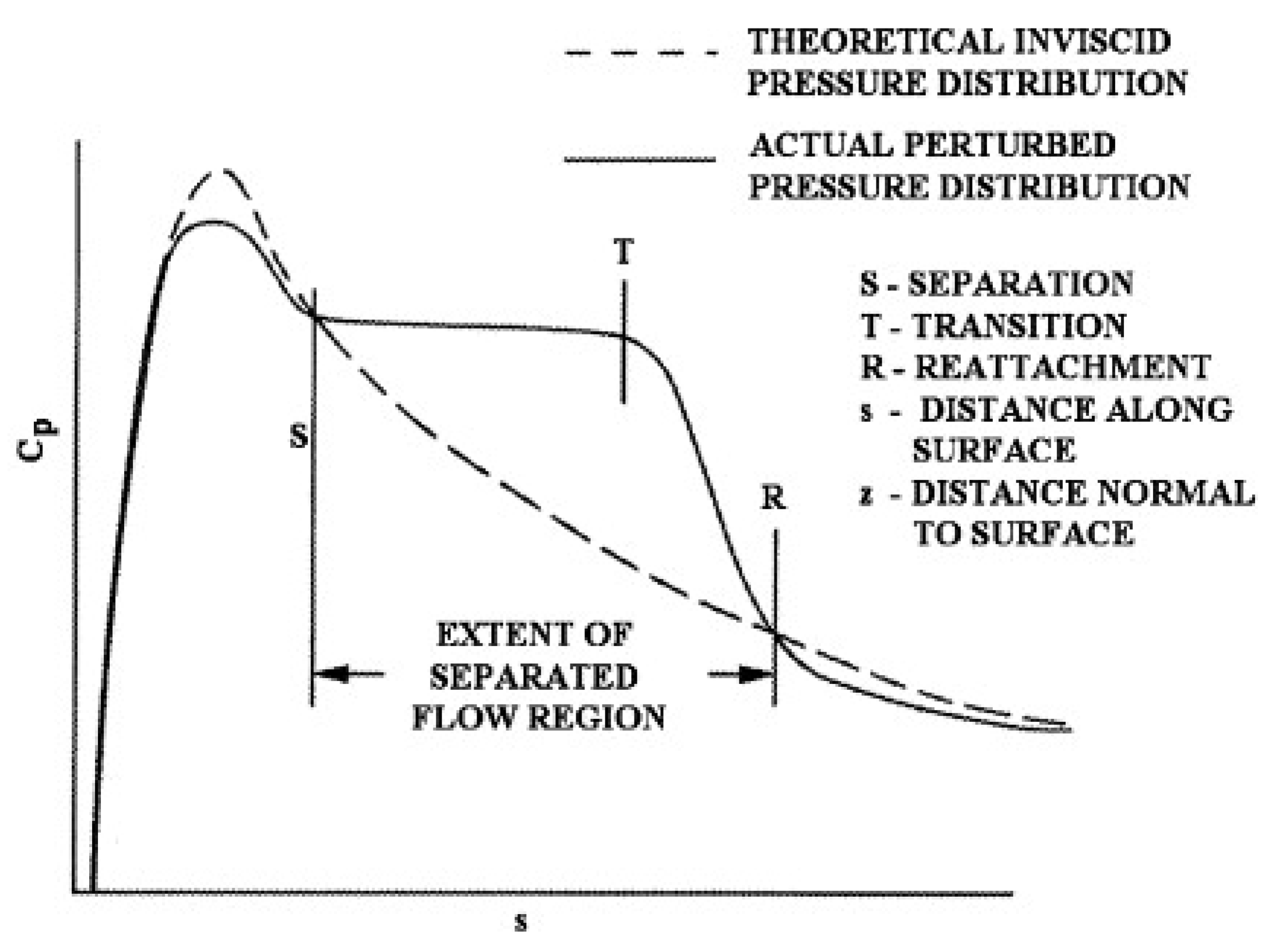
1.1. Laminar Separation Bubble (LSB)

During the transition of flow from laminar to turbulent flow, the surface of the laminar boundary layer that was previously attached begins to detach from the surface because of unfavorable pressure gradients. It then reattaches itself at a certain downstream location, thus resulting in the creation of LSB [2]. These separation bubbles have the potential to modify the flow field and the effective geometry of the airfoil, where they are more likely to occur on the suction surface. Even slight modifications in the geometry and operational parameters can significantly impair the performance of low R e airfoils. Those separation bubbles are more likely to be observed on the suction side of the airfoil with the potential to modify both the effective curvature of the airfoil and the flow field’s behavior. Airfoils designed for low Reynolds numbers are highly sensitive, and even minor modifications to their geometry and operating conditions can result in a mortification of their performance. LSB significantly influences the distribution of pressure, shear stress, and heat flux, thereby influencing the moment values, lift, drag, and nature of stalling of airfoils [10,11]. Jones [11] documented the presence of LSBs in 1934 as part of his experimental inquiries into the stalling characteristics of aircraft wings. Subsequent researchers conducted numerous experimental investigations in an effort to comprehend the behavior and form of LSB; a comprehensive compilation of these research studies is available in reference [12]. The research conducted by Horton [13] in 1968 yielded valuable insights into the physical mechanisms underlying the expansion and rupture of the bubble. As shown in Figure 1, he also postulated a fundamental structure for the LSB. At point S , the laminar boundary layer becomes detached from the surface of the airfoil. At point T , the flow transition from laminar to turbulent occurs, which takes place at the maximal height of the separation bubble. Eventually, turbulent mingling eliminates the reverse flow in the vicinity of the wall, and at point R , the flow reattaches. These are referred to as ‘short laminar separation bubbles’, and their impact on the pressure distribution is confined to a local area. A ‘short’ bubble can, however, expand and ‘burst’ into a ‘long laminar separation bubble’ in response to an increase in the angle of incidence or a velocity decrease. Long bubbles may persist as an ‘unattached free shear layer’ or reattach at a considerable downstream location, both of which significantly impact the distribution of pressure on a global scale [2]. The airfoil’s stalling behavior is determined by the nature of its bursting.

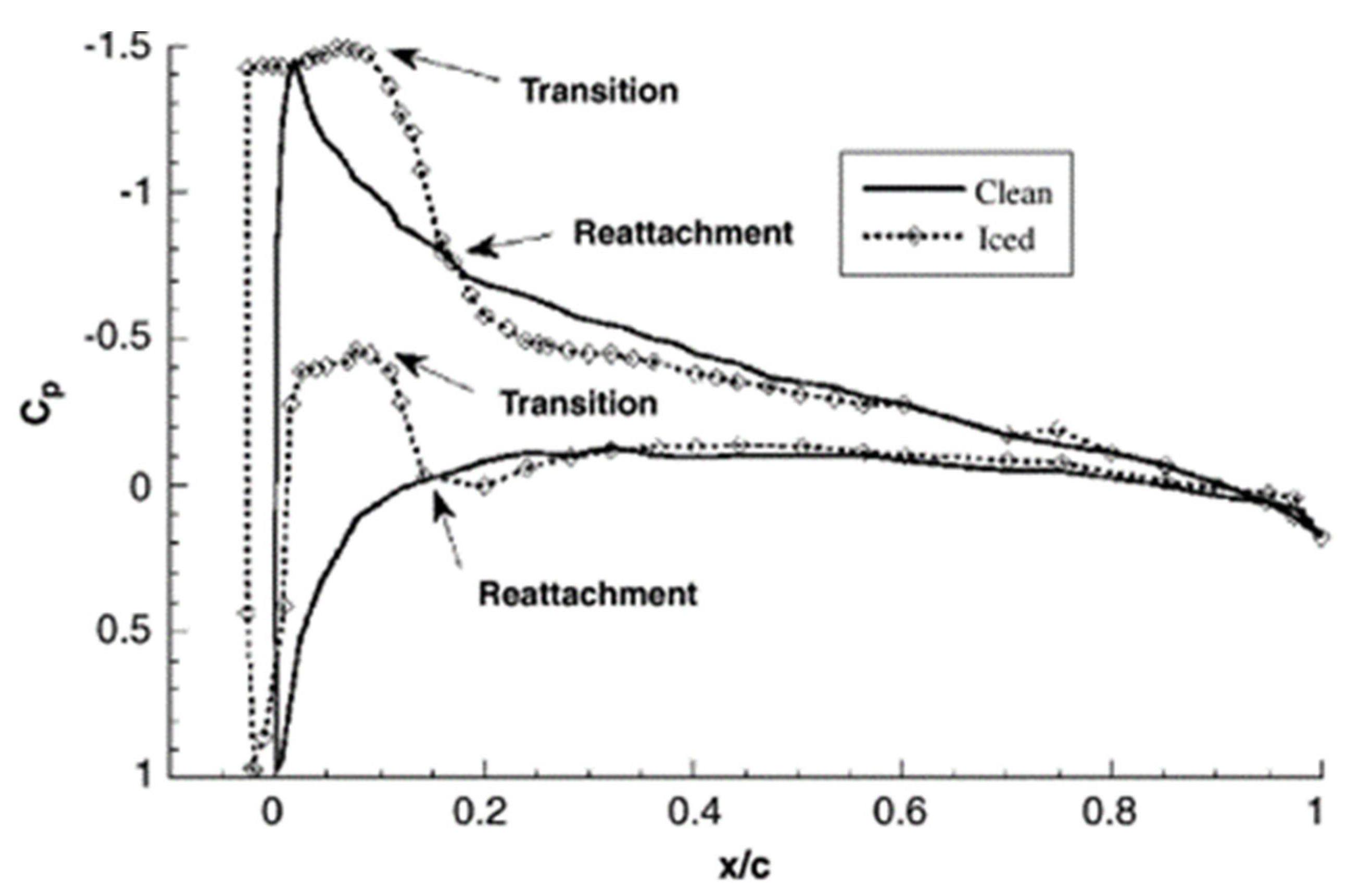
1.2. Ice-Induced Separation Bubble (ISB)

The adverse effect of ice accretion on the aerodynamic performance of an airfoil was initially reported in the studies of Gray [15] on NACA airfoils in 1953. Ice accretion on the leading side of the airfoil leads to significant performance losses like a decrease in lift and an increase in drag and is widely studied in the literature [16,17,18,19]. These studies were limited to the measurement of lift, drag, and moment on the iced airfoils only, and they lack information about the flow over iced airfoils. Later, from 1953 onwards, Bragg et al. [20,21,22,23,24,25] conducted a sequence of studies to understand the nature of the flow field in the vicinity of an iced airfoil. Measurement of the surface pressure was performed to understand the regions of flow separation, focusing on the location of separation, the reattachment point, and the length of the bubble [22,25]. The presence of an ISB was visualized for the first time by Bragg et al. [20] in 1984 using the oil flow visualization technique. In 1985, he [26] measured the time-averaged vertical velocity profiles inside the glaze ISB using split hot film measurements. The stagnation streamlines and dividing streamlines are traced using the measured velocity profiles, thereby providing the profile of ISBs at different angles of attack. In 1986, he [21] extended the studies using densely distributed surface pressure probes to study ISBs in detail. In the bubble zone, a nearly constant but slightly dropping pressure is followed by a pressure recovery region. The region of constant pressure can be considered the separated flow zone and the flow reattachment is expected to occur in this pressure recovery region. In 1992, he [24] concluded that the behavior of ISBs is quite similar to that of the LSBs in that the boundary layer transitions into turbulent flow with reattachment. Gurbacki [27] observed in 2002 that the reattachment location of the ISB varies as a function of time due to the inherent unsteadiness in the flow, leading to a reattachment zone, as shown in Figure 2. The length of the reattachment zone increases with an increase in the angle of attack, attributed to higher levels of flow unsteadiness.
Numerical studies about the aerodynamics of iced airfoils were extensively reviewed by Stebbins [29] in 2019 and are not intended to be repeated in detail here. Most of the numerical studies were performed on wings with leading-edge horn Ice accretions [30,31,32,33,34,35,36,37,38,39,40] and spanwise ridge ice [41,42,43]. Baldwin–Lomax (BL) and the Spalart–Allmaras (SA) model for turbulence were the widely employed turbulence models in studies with horn ice. The separation extent is overpredicted by RANS models, especially at angles of attack equal to and above 6 degrees, indicating that the accuracy of prediction decreases with an increase in the length of the separation bubble [29]. The numerical simulation predicted very high local suction peaks in the C p distribution, whereas the experimental results are smooth. Further, there were discrepancies in the prediction of surface pressure recovery on the pressure side. For the spanwise ridge ice, all the RANS-based studies were performed using the SA model. The distribution of pressure on the pressure side is accurately predicted, whereas the predictions of the same on the suction side were poor. For both ice shapes, RANS models predict the aerodynamic coefficients with reasonable accuracy in the linear-lift region but fail at higher angles of attack due to massive flow separation. Most of these studies were performed at Reynolds numbers in the order of 10 6 and Mach numbers above 0.1. However, the operating Reynolds numbers of UAVs range from the higher end of 10 4 to the lower end of 10 6 , and the flow field is predominantly laminar at these Reynolds number ranges. Not many studies were performed at these Reynolds number ranges to study the behavior of ISBs. The existing studies were limited to SA and BL turbulence models, and the capability of other RANS-based models has not been studied. The behavior of the ISB at low-Reynolds-number flows and the need for transition-based models in these flow regimes also need to be evaluated.

1.3. RANS-Based Turbulence Model for Prediction of LSBs and ISBs

The laminar-to-turbulent transition of the boundary layer has a significant impact on the flow characteristics. The distribution of shear stress and heat flux on the wall can also be thought of as a function of the location of turbulence onset and the length of transition regions. The transition process can also affect boundary layer separation behavior and the aerodynamic behavior of airfoils [44]. A major limitation of the existing numerical models is their inability to incorporate all those transition effects into a single model. Another issue stems from the fact that the transition process involves both linear as well as nonlinear effects, but the averaging technique used in Reynolds Average Navier Stokes equations (RANS) eliminates the effects of non-linear disturbance growth. Further, most transition models are based on non-local formulations as they use information about the flow variables outside the boundary layer and the integral thickness of the boundary layer. The dependence of transition models on non-local flow variables precluded its compatibility with existing CFD models. Modern CFD algorithms are incapable of computing integral boundary layer parameters due to their formulation based on unstructured grid and domain decomposition methods. Even though stability-based methods like the e n method [45,46] can eliminate these limitations, the requirement of prior knowledge of the grid and geometry also limits their application.
High-Reynolds-number turbulence models can often be used to predict the transition using two unique approaches. The incorporation of additional low-Reynolds-number model approximations is one option for managing turbulence formation during transitions. In order to address the implications of diminished turbulence intensity within a viscous sublayer, the equations incorporate damping functions. Despite the development of numerous low R e -turbulence models throughout the years [47,48,49,50], their capacity to predict the transition phenomenon appears to be coincidental and, hence, untrustworthy [44]. The second approach is to model the transition process as a mixture of laminar and turbulent flow in proportions that vary with the intermittency factor ( γ ). The value of γ ranges from 0 at the start of the transition to 1 at the end, and the overall flow could be γ times turbulent and ( 1 γ ) times laminar [51]. This method necessitates empirical information regarding the position of transition initiation and the exact streamwise variation of γ . These correlations relate the transition Reynolds number based on momentum thickness ( R e θ t ) with local variables like the turbulence intensity T u and the pressure gradient ( λ θ ) . Dhawan [52] in 1958 made such correlations as a function of the momentum thickness θ . In 1980, Abu-Ghannam and Shaw [53] proposed the empirical correlations for the prediction of the start and end of the transition by conducting experiments at different values of turbulence intensity T u and pressure gradient ( λ ) . Mayle [54] proposed correlations for zero-pressure-gradient flows in 1991, which are functions of T u and θ . In 1994, Gostelow et al. [55] proposed an empirical correlation for the streamwise distribution of intermittency, based on λ , T u , and θ . Steelant and Dick [56] proposed a transport equation for intermittency ( γ ) in 1996 and used it in conjunction with a conditioned Navier Stokes equation. The transition criteria are often associated with a two-equation turbulence model by an adjustment of the turbulent production term using an intermittency equation. The intermittency transport equation was incorporated into the k ϵ turbulence model by Cho and Chung [57] in 1992. In 2000, Suzen [58] coupled his intermittency transport equation with the SST k ω turbulence model. Most of these transition models are based on non-local formulations as they use information about the flow variables outside the boundary layer and the integral thickness of the boundary layer. To address these issues, Menter [44] proposed basic formulations of transition models based on local variables in 2002. In 2004, Menter [59] added a transport equation for the R e θ t to the SST k ω turbulence model and called it the γ R e θ t transition model. He introduced a local property called the vorticity Reynolds number ( R e V ). The value of the maximum vorticity Reynolds number in the profile of a boundary layer is directly linked to the momentum thickness Reynolds number. To induce the transition, the vorticity Reynolds number is used rather than the momentum thickness Reynolds number directly.

2. Numerical Methodology

In this study, the 2D-incompressible RANS equations were solved with a finite volume formulation called SIMPLE for the pressure–velocity coupling. For the spatial discretization of fluxes, a second-order accurate upwind scheme is used. The various turbulence models employed in this study are briefly discussed below.

2.1. Turbulence Model

The Spalart–Allmaras (SA) model [60] is essentially a low-Reynolds-number model that uses a one-equation transport model for solving kinematic eddy viscosity ( v ~ ) . The transport equation for the SA model is given below in Equation (1).
t ρ v ~ + x i ρ v ~ u i = G v + 1 σ v x j μ + ρ v ~ v ~ x j + C b 2 ρ v ~ x j 2 Y v + S v ~
where μ is the turbulent viscosity and G v and Y v are the turbulent viscosity production and destruction terms.
The turbulent kinetic energy k and the specific dissipation rate ω transport equations are solved in the standard k ω turbulence model as given in Equations (2) and (3). Because this model is sensitive to freestream conditions, an SST k ω turbulence model was proposed in 1994 by Menter [61]. This model combines the advantages of the k ε model [62] in the far field with that of the k ω model in the region near the wall [63]:
t ρ k + x i ρ k u i = x j Γ k k x j + G k Y k + S k + G b
t ρ ω + x i ρ ω u i = x j Γ ω ω x j + G ω Y ω + S ω + G ω b
where G k and G ω represent the generation of k and ω , respectively, due to the mean velocity gradients. Γ k and Γ ω represent the effective diffusivity of k and ω , respectively. Y k and Y ω represent the dissipation of k and ω due to turbulence. S k and S ω are user-defined source terms. G b and G ω b account for buoyancy terms.
The interaction of the transition model with the SST turbulence model occurs by modifying the terms G k and Y k in the k -equation as shown in Equations (4) and (5), respectively.
G k * = γ e f f G ~ k
Y k * = min max γ e f f , 0.1 , 1.0
where the original production and destruction terms for the SST model are represented by G ~ k and Y k . γ e f f physically represents the percentage of time the turbulent fluctuations are present in the boundary layer, and it varies between 0 and 1 by damping the production of turbulence in the laminar and transitional regions of the boundary layer. The damping limiter ensures that the dissipation rate does not drop below 10% of the turbulent value. The terms G k and Y K are modified as shown in Equations (6)–(8), such that:
G k * = 0     and   Y k * = 0.1   Y k   in   the   laminar   boundary   layer
0 < G k * < 1     and   Y k * = γ e f f   Y k   ( 0.1 <   γ e f f < 1 )   in   the   transitional   boundary   layer
G k * = 1   and   Y k * = Y k   in   the   turbulent   boundary   layer
The algebraic transition model formulates the intermittency as an algebraic equation instead of the transport equation for intermittency [63]. The algebraic equation is integrated into the k ω based turbulence models by multiplying intermittency ( γ ) into the production term p k . The empirical correlation is made in such a way that it fits the experimental transition locations.
γ = f ( R e θ C ,   R e v ,   T u ,   λ θ )
where R e θ , c is the critical Reynolds number where the intermittency first starts to increase in the boundary layer, T u is the turbulence intensity, and λ θ is the non-dimensional pressure gradient parameter. R e v is the vorticity Reynolds number defined as a function of the wall distance ( d w ) and strain rate magnitude (S).
R e v = ρ d w 2 S μ
The intermittency ( γ ) transition model [64] solves one transport equation for intermittency (see Equation (11)), where the production term controls the length of transition and the dissipation term allows the boundary layer to re-laminarize by dissipating the intermittency fluctuations. The momentum thickness Reynolds number is algebraically computed using local variables [64].
t ρ γ + x j ρ u j γ = x j [ μ + μ t σ γ γ x j   ]   + P γ E γ
The intermittency production term P γ 1 is given by Equation (12):
P γ 1 = F l e n g t h   ρ S γ 1 γ F o n s e t
where F l e n g t h is the empirical correlation that controls the length of the transition region and F o n s e t switches on the production of intermittency.
F o n s e t = f R e θ c ,   R e v , d w ,   ρ ,   k , 1 ω , 1 μ , s ,   T u ,   λ θ
F l e n g t h = 100
In order to account for the transition behavior, the transition k ω S S T turbulence model, also called the γ R e θ   t r a n s i t i o n   m o d e l [65], is coupled to the S S T   k ω model with a transport equation for intermittency and the transition Reynolds number. The former is given in Equation (15).
t ρ γ + x j ρ u j γ = x j [ μ + μ t σ γ γ x j   ] + P γ 1 E γ 1 + P γ 2 E γ 2
The intermittency production term P γ 1 is given by:
P γ 1 = F l e n g t h C a 1 ρ S γ F o n s e t C γ 3
E γ 1 = P γ 1 γ
Similarly, F o n s e t switches on the production of intermittency and F l e n g t h controls the length of the length of the transition region.
F o n s e t = f R e θ c ,   R e v , d w ,   ρ ,   k , 1 ω , 1 μ , s ,   T u ,   λ θ
F l e n g t h = f ( R e ¯ θ t )
R e θ C = f ( R e ¯ θ t )
R e θ t = f ( T u , λ )
R e θ , t is the transition Reynolds number where the transition occurs, and a transport equation is solved for R e ¯ θ t
t ρ R e ¯ θ t + x j ρ U j R e ¯ θ t = x j [ σ θ t μ + μ t R e ¯ θ t x j   ] + P θ t
Transport equations for turbulent kinetic energy ( k T ) , laminar kinetic energy ( k L ), and the inverse turbulent time scale ( ω ) is solved in the k k l ω transition model [66], which is classified as a three-equation eddy-viscosity type.
D k T D t = P k T + R + R N A T ω k T D T + x j [ υ + α T α k k T x j ]
D k L D t = P k L R R N A T D L + x j [ υ k T x j ]
D ω D t = C ω 1 ω k T P k T + C ω R f W 1 ω k T R + R N A T C ω 2 ω 2 + C ω 3 f ω α T f W 2 k T d 3   + x j [ υ + α T α ω ω x j ]
The effective diffusivity term in Equations (2) and (3) depends on the coefficient α * . A low R e correction damps the turbulent viscosity by modifying the coefficient α * .
α * = α * ( α 0 * + R e t R k 1 + R e t R k )
where R e t = ρ k μ ω and the remaining terms are constants.
The author intended to provide a very concise explanation of the turbulence models considered in this study, and many terms are not defined in detail. Reference [63] provides a full discussion of the numerous source terms, empirical relations, and constants employed in these turbulence models. Since all these turbulence models are based on many empirical equations and constants, researchers have shown that the finetuning of such constants can improve the predictions. However, it will remain case-specific and cannot be considered universal for industrial applications. Therefore, the numerical simulations in this research have been performed using the standard empirical constant recommended by Ansys [63] to find the best generic turbulence model for low-Reynolds-number studies.

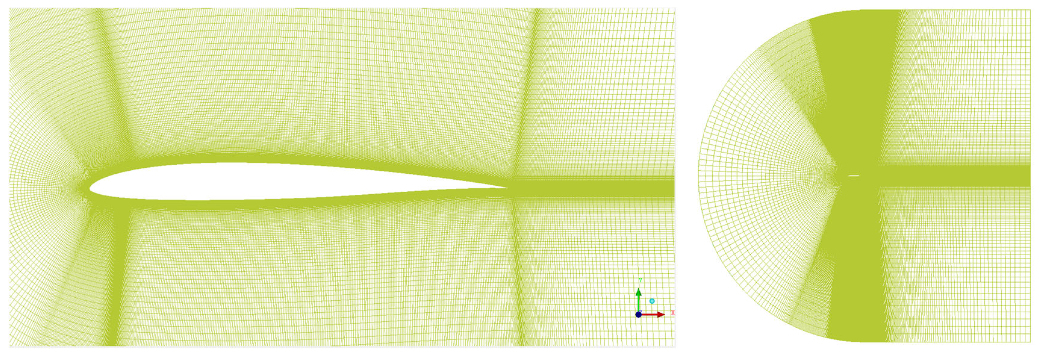
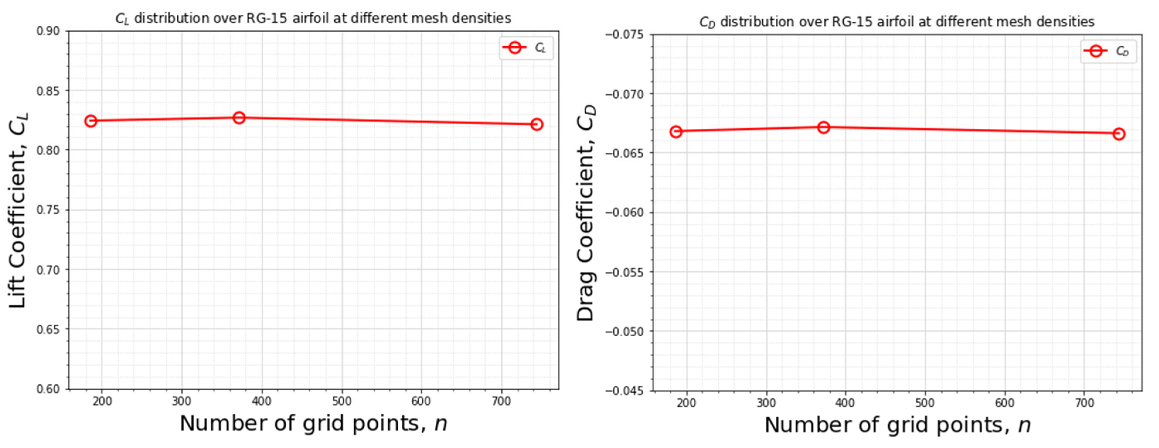
2.2. Computational Model

Computational simulations were conducted on the low-Reynolds-number airfoil Rg-15, which is well-suited for unmanned aerial vehicle (UAV) applications. The reference airfoil had a chord length of C = 210   m m , resulting in 1.07 × 10 5 Reynolds number at 7.25   m / s velocity. The ice shape was adopted from the studies of Williams [67], and the experimental data about LSBs and ISBs are derived from the research of Oo et al. [6]. Numerical simulations were run using the Ansys FLUENT program v18.2, a widely used commercial tool. Multiblock structured 2-D C-grid was made using the software called ICEM CFD, following the guidelines outlined in reference [63] for transition models. The flow domain stretches from the leading edge in all directions for ten times the chord length. To guarantee that the Y-plus value stays below 1, the first cell with a height of 1 × 10 6 is used, and the computation mesh is massed in the streamwise directions. Grid independence studies are conducted to verify that the separation bubble is unaffected by changes in the grid resolution, as shown in Figure A1 of Appendix A. The computation utilizes a numerical grid consisting of 231,032 cells (371 grid points on the airfoil surface), as depicted in Figure 3. The simulations were conducted for a significant number of iterations to guarantee the convergence of force coefficients, precision in LSB location, and the fall of residuals to a value significantly below 1 × 10 6 . The research was conducted for 0 ,   3 ,   a n d   6 o angles of attack, and its findings match the literature data [6]. Turbulence intensity can be considered a crucial aspect influencing the LSB. A wind tunnel with a turbulence level of 1.2% is used for experimental testing and, therefore, the same value is also employed for numerical research. A comparison of the predictions of LSBs using steady-state and time-averaged simulations is shown in Figure A2 of Appendix A. Detailed comparisons can also be found in the earlier research works of the author [68]. At lower angles of attack, the differences in the predictions of steady-state and time-averaged simulations are negligible. Therefore, considering the computational cost, steady-state simulations are performed here. The experiments were performed in the literature on a 2D infinite wing, and therefore, the simulations are also performed in 2D for one-to-one comparisons. The above-mentioned simplifications are adopted since the goal of this study is to assess the capacity of different models to predict LSBs and ISBs. However, from a physics perspective, these separations are three-dimensional and unsteady.

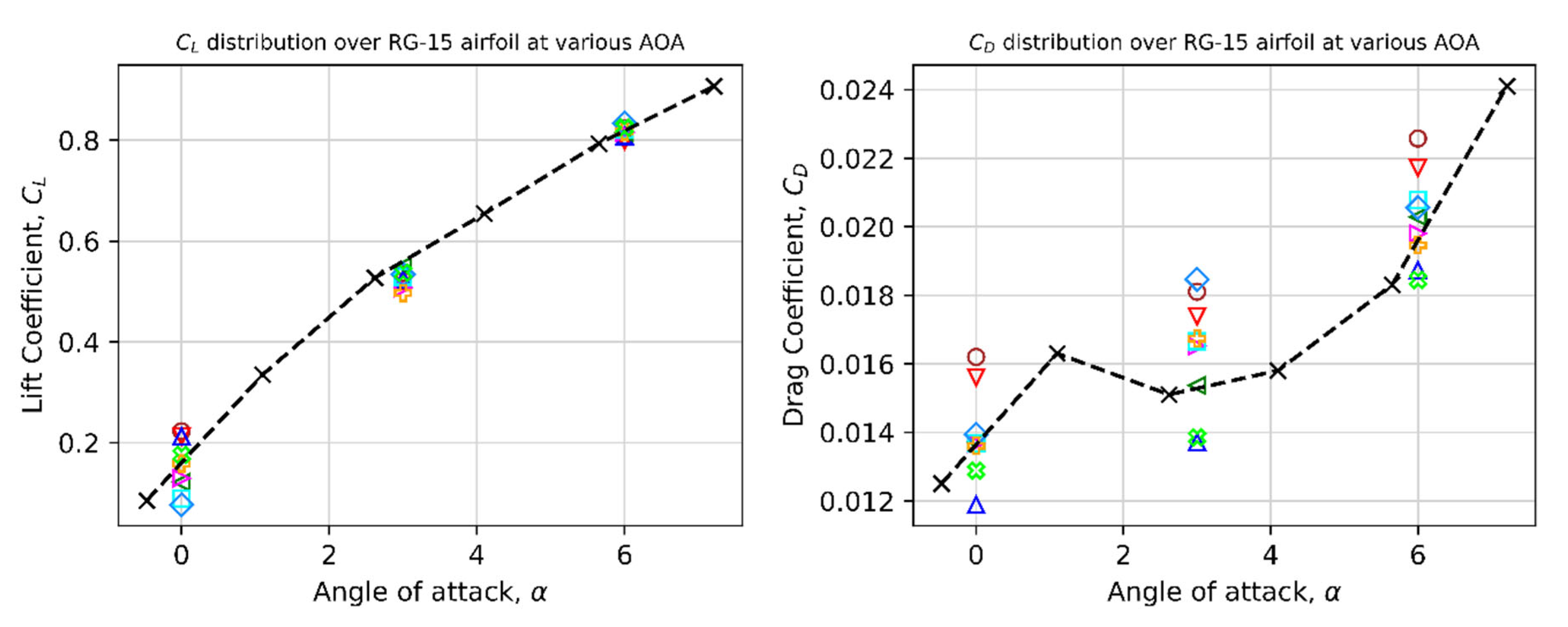
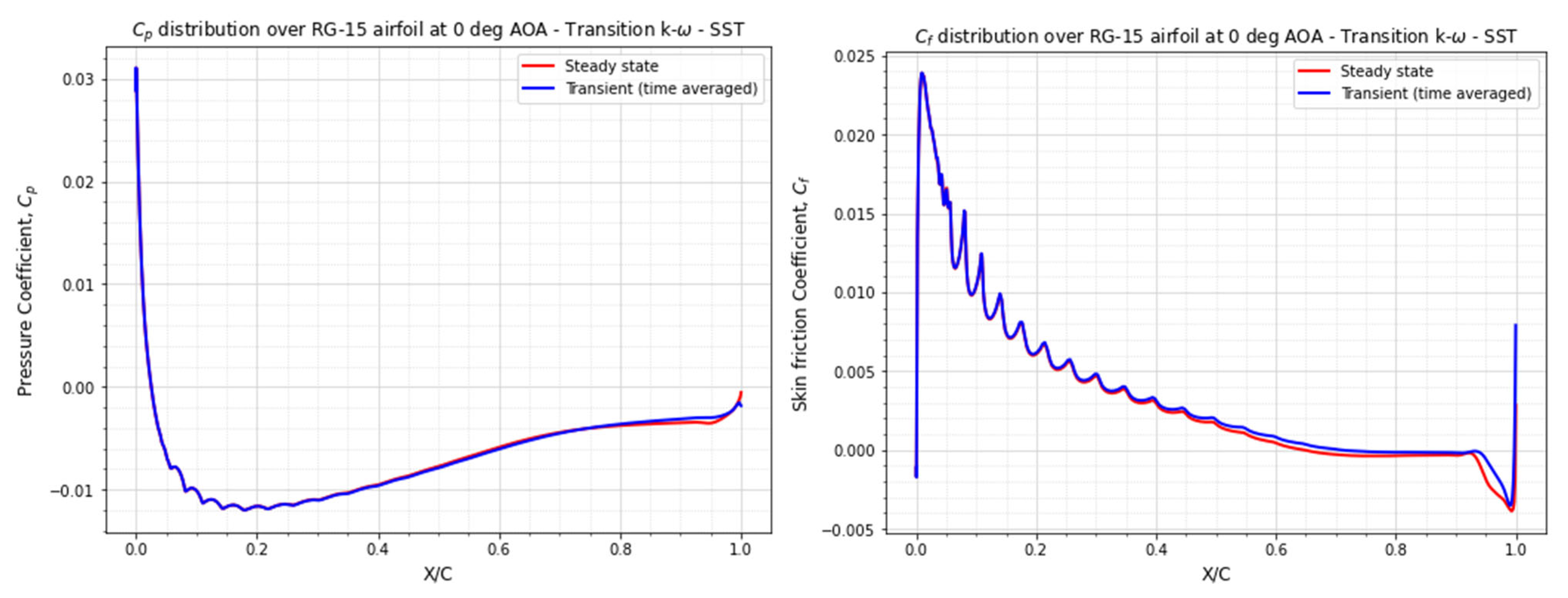
3. Results and Discussion

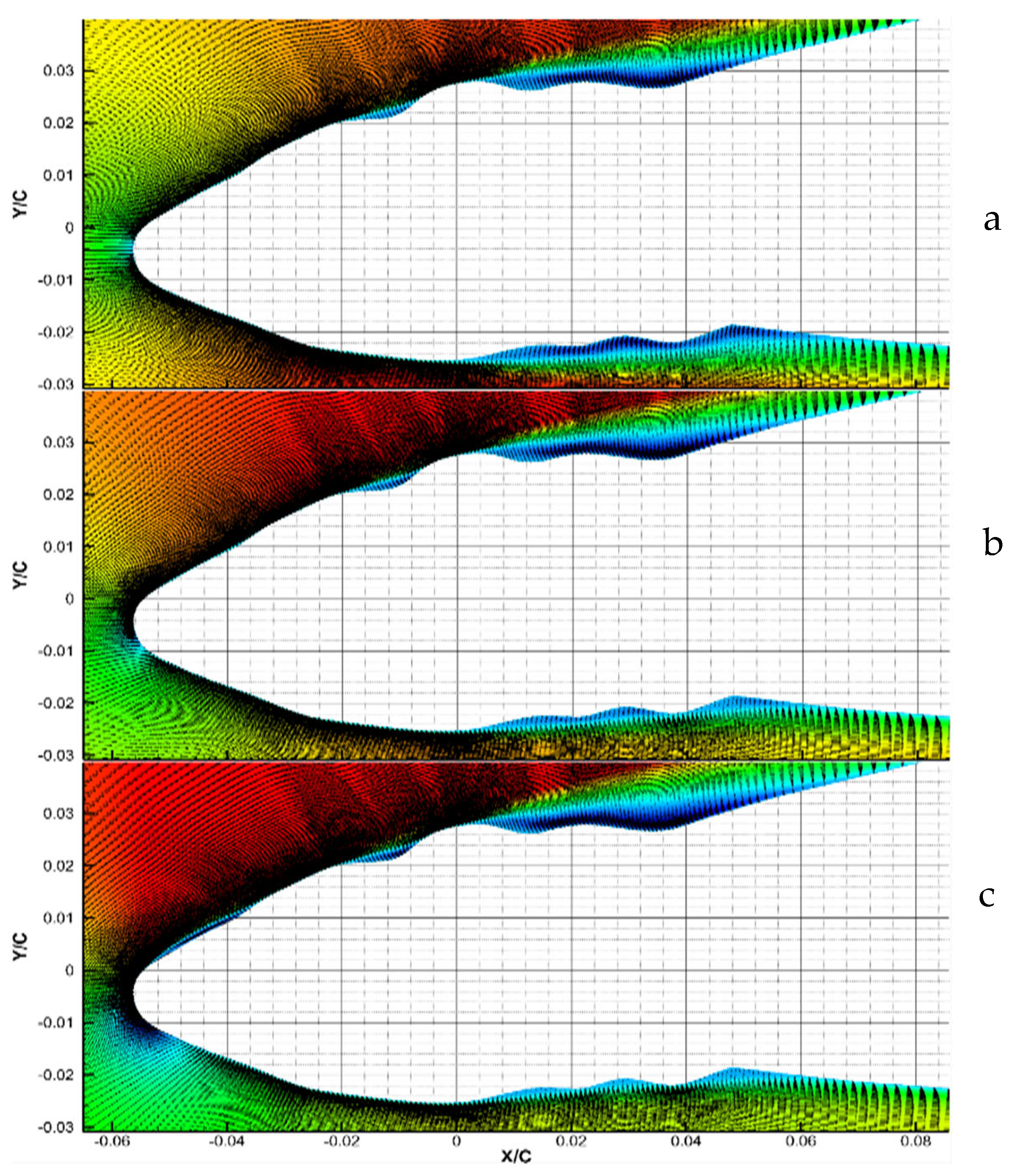
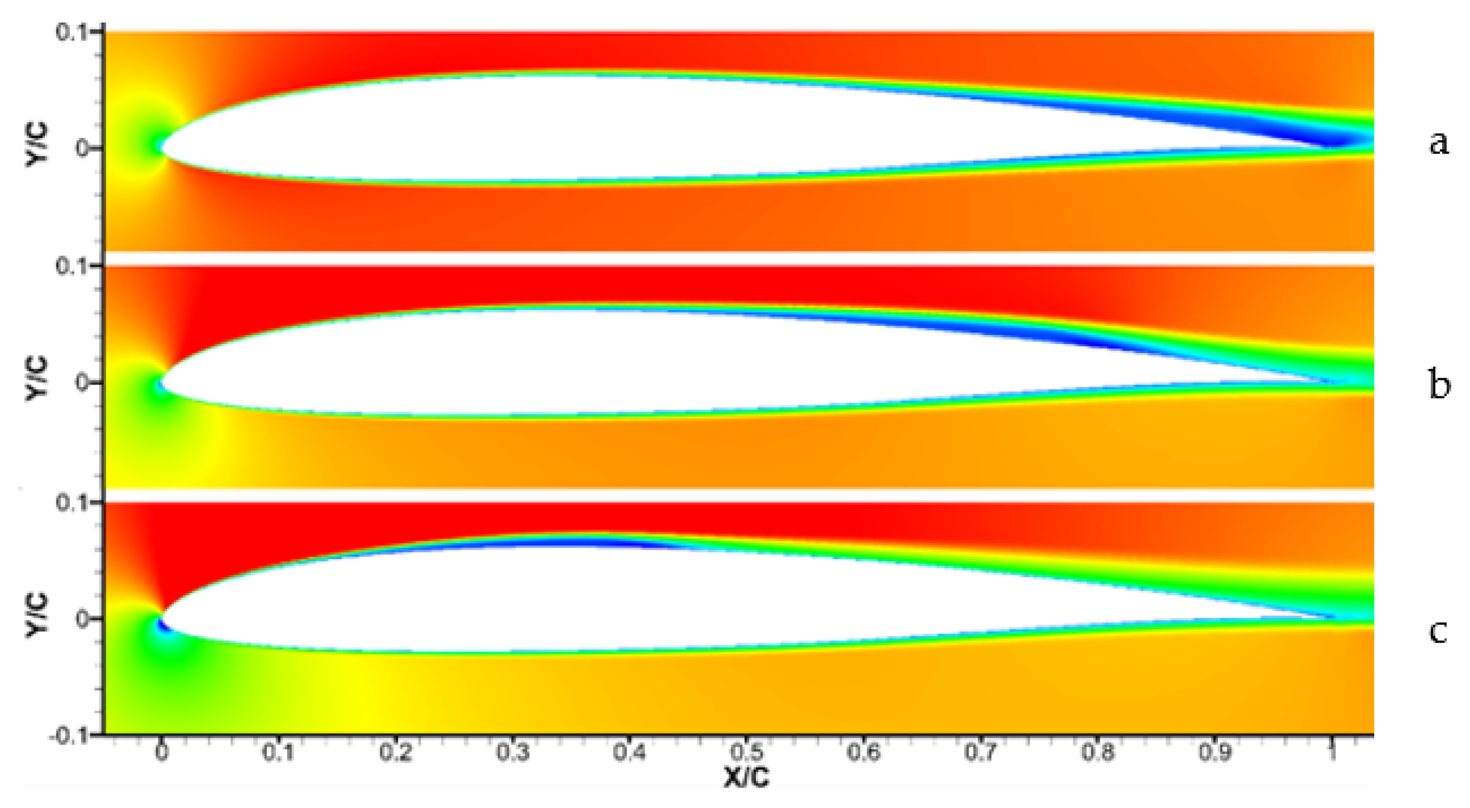
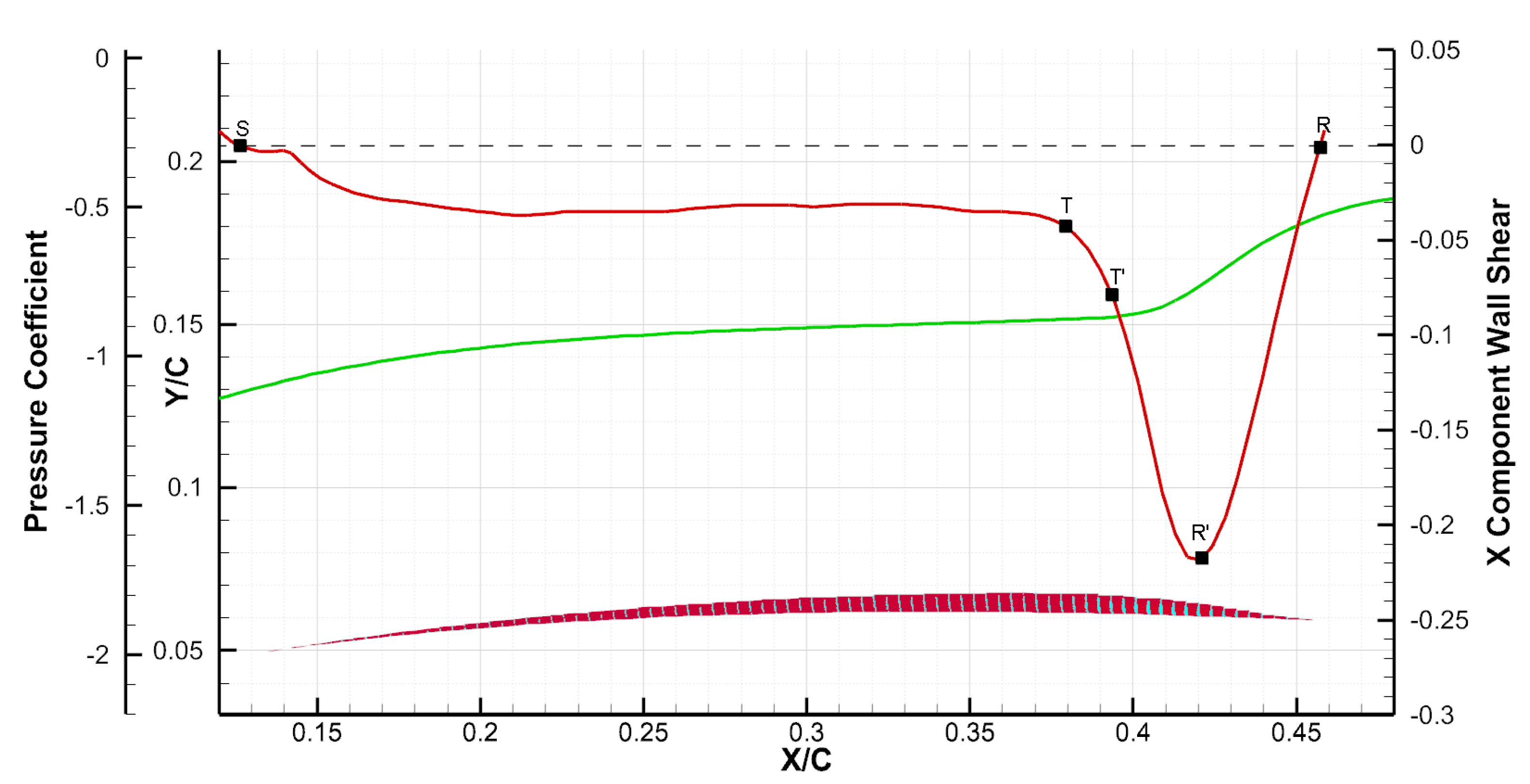
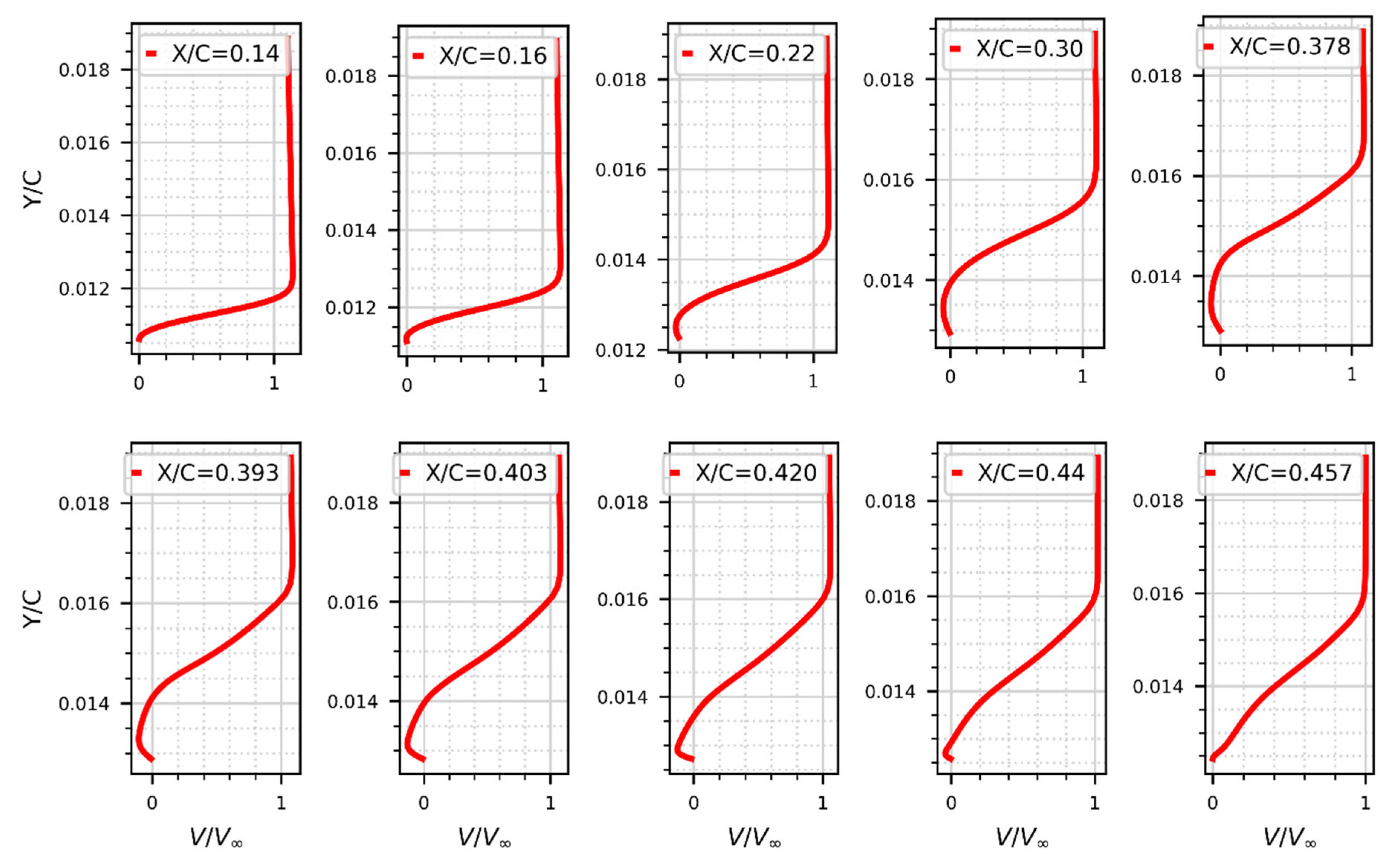
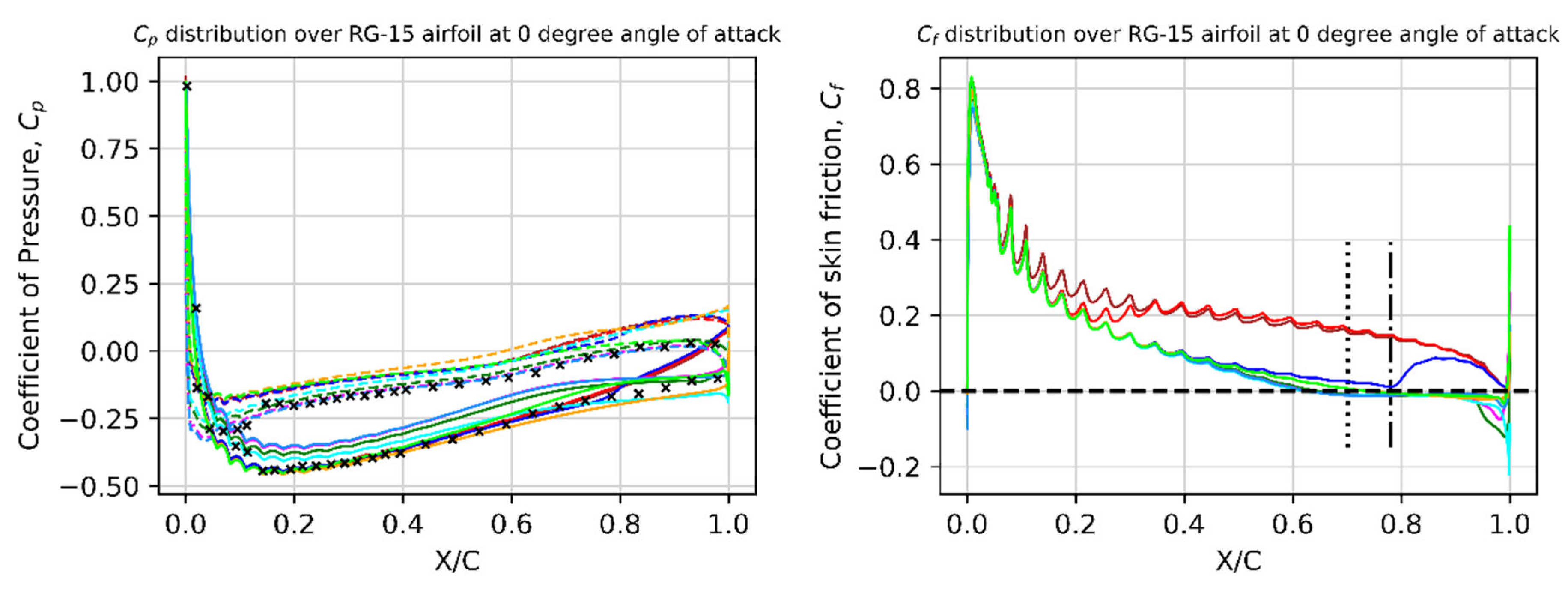
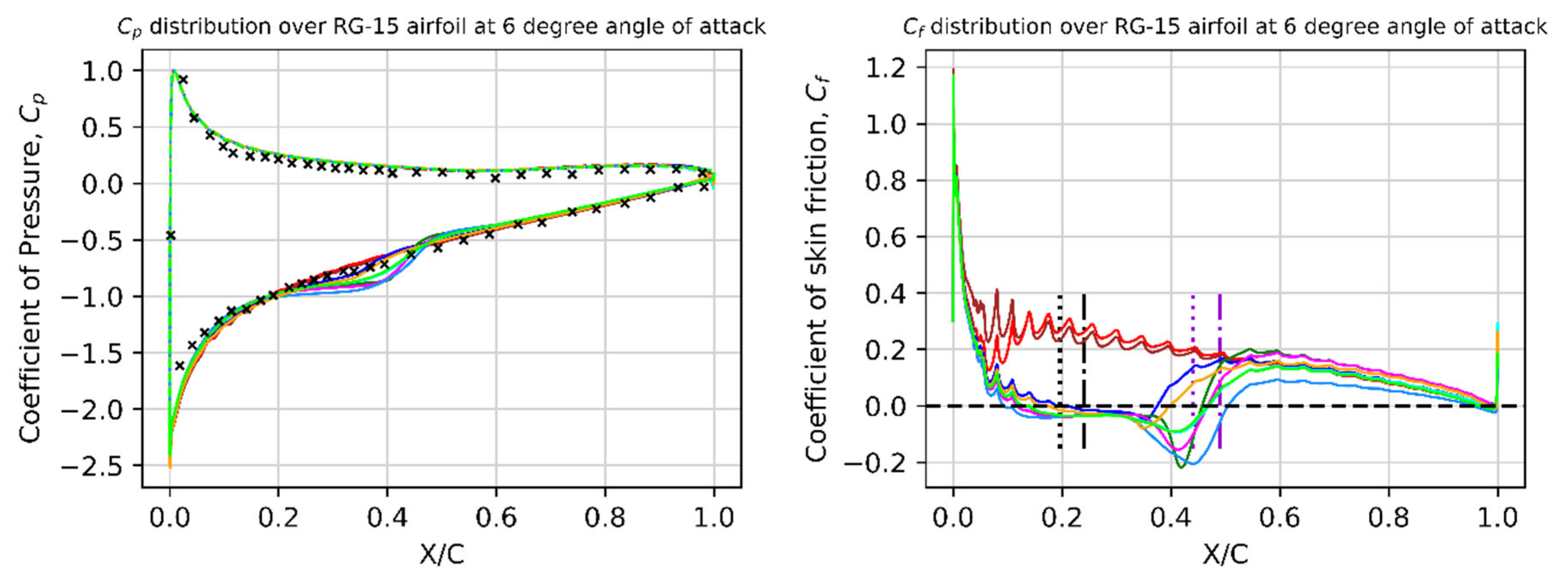
3.1. Laminar Separation Bubbles (LSBs)

Figure 4 depicts the traits of LSBs as the angle of attack on the RG-15 airfoil surface increases. At an angle of attack of zero degrees, the boundary layer detaches from the surface close to the airfoil trailing edge and does not reconnect to the surface of the airfoil, thus resulting in an open-type LSB. An upstream movement of the separation onset is observed with an increase in the angle of attack to 3 degrees. Also, the flow reattaches to the airfoil surface, resulting in a closed-type LSB. The separation onset travels upstream with a decrease in length and thickness when the angle of attack changes to six degrees. In experiments, the presence of an LSB is detected utilizing the C p distribution curve [24,69] as shown in Figure 5. Due to the same pressure within the separated flow regions, an LSB is denoted by a flattening of the C p distribution curve. The initiation of separation is denoted by the beginning of C p flattening, and the termination of flattening is designated as the transition point. The instant at which the C p value returns to its inviscid state is considered the juncture of reattachment.
The value of coefficient of skin friction ( C f ) is negative inside the separation bubble due to the reverse flow, and it can be used to distinguish the regions of flow separation [70]. However, the C f curve is not examined in detailed like the C p distribution curve. Thus, an attempt is made here to study the geometry of LSBs from the C f curve. Figure 6 shows the LSB, C p distribution, and C f distribution over Rg-15 at a 6-degree angle of attack predicted by the γ R e θ transition model. The γ R e θ transition model is chosen because of its closer agreement with experimental results as discussed in Section 3.2. The point where the C f curve initially crosses zero is considered the point of separation onset and, therefore, the location denoted by ‘ S ’ in Figure 6 could be considered the location of separation onset. After the separation onset, the thickness of the bubble gradually increases and the magnitude of negative C f also increases up to some point before it remains flat until point ‘ T ’ (X/C = 0.378). C f is a function of the gradient of velocity in the direction normal to the wall, and an increase or decrease in the velocity gradient is responsible for the sudden variations in C f , as shown in Figure 6. Compared to a laminar boundary layer, velocity increases more rapidly in the direction normal to the wall within a turbulent boundary layer. Consequently, the profile of the turbulent boundary layer is exponential, whereas the profile of the laminar boundary layer is parabolic instead. In laminar flow, the free-flowing fluid’s kinetic energy is transferred to the slower-moving fluid at the surface solely by viscosity, i.e., frictional shear stresses. There is no entrainment of energy from the mean flow into the boundary layer observed in the laminar region of the separation bubble [71]. Therefore, the fluid inside the laminar part of the separation bubble is recirculating at a reduced velocity. In a turbulent flow, the kinetic energy of the mean free stream is entrained into the boundary layer and, therefore, the fluid gains more energy and its velocity increases. The velocity profiles along the airfoil surface at specific chordwise locations are shown in Figure 7. The velocity magnitudes are normalized by the local velocity of the main flow, and the chordwise positions are normalized by chord length. For the positions upstream of the maximum thickness point in LSBs (T, X/C = 0.378), the reverse flow velocity profile is parabolic in nature, and after point ‘T’, it becomes exponential. Thus, during the onset of LSB, there is a small velocity gradient due to the development of reverse flow, and because the velocity gradient is smooth in a parabolic profile, the C f remains relatively flat. At point ‘ T ’, the LSB has attained the maximum thickness, and it can be considered the start of the transition process. The laminar-to-turbulent transition can be considered as a process that occurs over a finite distance and, therefore, it cannot be defined at a specific point [70]. The “Transition zone” could be considered a better expression than the transition location or transition point when speaking about flow transitions. The sudden fall in the C f value (sudden increase in the negative C f value) is an indication of a full transition and is denoted by the letter ‘ T ’ in Figure 6. From Figure 7, it can be observed that the profile of the reverse flow starts to become exponential at point ‘T’ (X/C = 0.378), and the gradient becomes sharper at point ‘ T ’ (X/C = 0.393). Therefore, the region ‘ T T ’ can be considered the transition zone. The entrainment of energy from the mean flow develops a greater velocity gradient in the turbulent region of the bubble, and the C f value increases rapidly up to point ‘ R ’. After this point, the velocity gradient decreases until the flow reattaches at Point ‘ R ’.
The slope of the ‘ R R ’ curve depends on the rate of entrainment of energy from the mean flow. The entrained fluid rolls up into vortices and is then propagated downstream by shedding vortices, so no apparent reverse flow layer is observed [71]. This entrainment, combined with the favorable pressure gradient and the shear layer’s dominance over the region of “dead fluid”, allows the boundary layer to quickly reattach and form a bubble. The fluid flow appears to be very smooth and orderly after reattachment, with vortex structures stretching as they are connected downstream [72]. It could be noted from the C p distribution curve that the region inside the bubble is not completely flat and is increasing at a slower rate. Also, it can be observed that, at the beginning of the LSB, the C p distribution is not affected much, and the effect starts to be revealed after the LSB has gained some thickness. Therefore, using the C p distribution curve to measure the separation and reattachment point has its limitations. In the C f graphs presented in this manuscript on Section 3.2 and Section 3.4, the black dashed horizontal line represents the C f = 0 line and the black dash-dotted and dotted vertical lines represent the experimental and LES predictions of the separation onset, respectively. In a similar way, the purple lines represent the reattachment locations. The LSB is predicted only on the suction side of the Rg-15 airfoil in both the experiments and numerical simulations.

3.2. Fidelity of RANS Models in Predicting Laminar Separation Bubbles (LSBs)

The efficiency of various turbulence models based on RANS equations in modeling the LSB is studied by conducting numerical simulations using nine different RANS-based turbulence models. The characteristics of the LSB over the RG-15 airfoil were studied by Oo et al. [6] in 2020, and large eddy simulations were performed to predict the location of LSBs and validated with experimental studies in a wind tunnel. The Cp distribution over the RG-15 airfoil at various angles of attack (0, 3, and 6 degrees) is reported in his work along with the separation onset and reattachment location of LSBs. The fidelity of each turbulence model in predicting the LSB is analyzed using three different parameters: the C p distribution, separation onset, and reattachment point from the C f distribution and aerodynamic coefficients. The separation onset and reattachment are calculated in the literature using C p distribution curves; therefore, it has limitations in predicting the exact locations as discussed in section A. The aerodynamic coefficients ( C L and C D ) values are based on the shear stress and pressure distribution on the airfoil surface. C L values mainly depend on the difference in mean pressure on the pressure side and suction side of the airfoil and, therefore, it is relative. Therefore, using C L and C D values in assessing the prediction of a turbulence model is trivial. As a result, in this study, weightage is given to the C p distribution more than other factors as a mandate to assess the performance of the turbulence model.
The C p profile over Rg-15 for nine different RANS-based turbulence models at 0-degree angles of attack is shown in Figure 8. Only the transition turbulence models are capable of capturing the C p distribution accurately. Also, it can be observed that a negative value of C f (indicative of separation) is predicted only by the transition turbulence models. Therefore, the conventional RANS turbulence models failed to predict the LSBs, while transition-based models succeeded. Upon comparing the C p and C f distributions predicted by the numerical models with experiments, it can be observed that all the models predict the early onset of separation when compared to experiments. It should also be noted that even the LES simulation results (obtained from the literature) also predicted the early onset of the separation bubble. The γ R e θ transition model, the γ transition model, and the K K l ω model predict the C p distribution accurately on the pressure side of the airfoil. However, these models overpredicted the C p predictions on the suction side of the airfoil. Also, it should be noted that the C p plateau predicted by numerical simulation is very distinct, but the C p predictions in the separation region from experiments have a slight positive slope. This may be due to the fact that the separation bubble predicted by these transition models is stronger (large velocity gradients) than the actual LSBs observed in experiments. Introducing the low-Reynolds-number correction to the γ transition model corrected this problem, but then the pressure side C p was overpredicted. In contrast with other transition models, the algebraic transition model predicted an LSB of low strength and, therefore, the C p distribution on the suction side has a better match with experiments. However, this model overpredicted the C p on the pressure side. Introducing the low-Reynolds-number correction to this model improved the overall C p predictions, but still the C p on the pressure side is overpredicted. This is because these models predicted a trailing edge separation bubble on the pressure side of the airfoil, which is not observed in the experimental and LES studies. Overall, the C p predictions of the γ R e θ transition model and the γ transition model are closer to experimental prediction provided the C p on the suction side is overpredicted. Table 1 shows the comparison of separation and reattachment positions of each transition model with experimental and LES observations. The separation onset is modeled more closely using the experimental predictions of the algebraic transition models with and without low R e correction. However, as mentioned before, these models predicted non-physical separation bubbles on the pressure side. The γ R e θ transition model has the next closest prediction when compared with experiments with an error of 6.41%.
Figure 9 shows the C p and C f distribution over Rg-15 at a 3-degree angle of attack. In contrast with the observations made at a 0-degree angle of attack, the overall C p predictions of both the conventional and transitional turbulence models show a close match with the experimental predictions. All the models slightly overpredicted the C p on the pressure side and it shows deviations at the region of LSB. Similar to the 0-degree case, the C p predictions of conventional RANS models on the suction side are in line with the experimental measurements forward of the separation zone, but they deviate inside the recirculation zone due to its inability to predict LSBs. It can be observed from the C f distribution that all γ R e θ only transition models and algebraic transition models predict a separation bubble that reattaches to the surface of the airfoil (the same is also observed in experiments). Similar to the zero-degree case, the γ R e θ transition model predicted a strong separation bubble and, therefore, C p is slightly overpredicted locally in the LSB zone. The origin of the separation is accurately predicted by both models, but the reattachment point is predicted accurately by the γ R e θ transition model only.
When the angle of attack is increased to 6 degrees, the size of the LSB is reduced and its effect on overall C p distribution is more localized as shown in Figure 10. Except inside the LSB, the C p predictions of the numerical simulations and experiments are quite comparable. The conventional models failed to predict the LSB, and all of the transitional models predicted a stronger separation bubble than the one in the experiments. Therefore, C p is overpredicted by transition models in the LSB zone but is slightly underpredicted by conventional RANS models. From the C f distribution shown in Figure 10 and the information given in Table 1, it can be observed that all the transition models predict a closed LSB that reattaches to the airfoil surface. Most of the transition models predict the separation much earlier, when compared to experiments. The conventional k ω S S T turbulence model with low R e correction and the algebraic transition model have better predictions of the separation onset location, but these models predict much earlier reattachment. Other transition models predict a reattachment location that is in between the predictions of experiments and LES, except the k k l ω model, which has a reattachment location aft of the experimental reattachment point. The legend for Figure 8, Figure 9, Figure 10 and Figure 11 is given in Figure 12.
Figure 8. C p (left) and C f (right) distribution over Rg-15 airfoil at 0-degree angle of attack (See Figure 12 for legend).
Drones 08 00148 g008
Figure 9. C p (left) and C f (right) distribution over Rg-15 airfoil at 3-degree angle of attack (See Figure 12 for legend).
Drones 08 00148 g009
Figure 10. C p (left) and C f (right) distribution over Rg-15 airfoil at 6-degree angle of attack (See Figure 12 for legend).
Drones 08 00148 g010
Figure 11. C L (left) and C D (right) distribution over Rg-15 airfoil (See Figure 12 for legend).
Drones 08 00148 g011
Figure 12. Legend for Figure 8, Figure 9, Figure 10 and Figure 11.
Drones 08 00148 g012
Upon comparing the C p distribution at the three angles of attack considered in this study, it can be observed that the occurrence of laminar separation bubble has altered the C p distribution on the entire airfoil surface (both pressure and suction sides). For the 3-degree case, the influence of LSBs on the C p distribution outside the LSB is considerably reduced and is negligible for the 6-degree case. Thus, the open separation bubble formed in the 0-degree case has a global effect on the C p distribution and can be considered a “long LSB”. The bubbles formed at 3-degree and 6-degree angles of attack have only a local influence on the C p distribution (mainly in the separated flow zone) and can be considered “short LSB”. The thickness of the separation bubble at the onset of separation is very small and increases quite gradually, thus increasing the chances of experimental uncertainties in predicting the separation onset of an LSB. Previous researchers also reported that the LSB is quite unsteady and the reattachment point fluctuates, leading to a reattachment zone [27]. Therefore, considering the prediction of the reattachment location and C p distributions, the performance of the γ R e θ transition model classified it as a better model compared to the various transition-based models for the study of LSBs at lower angles of attack.
Figure 11 shows the C L and C D predictions of the nine different turbulence models considered in this study for all three angles of attack. The experimental C L and C D values are obtained from the studies of Selig [73] for R e = 10 5 . It can be observed that LSB has a considerable influence in the prediction of aerodynamic coefficients. For zero-degree angle of attack, the algebraic transition models with and without low R e correction have the closest match with experimental predictions followed by the γ and γ R e θ transition models. For 3-degree angle of attack γ R e θ transition models have the best prediction and for 6- degrees the algebraic transition model, γ and γ R e θ transition models predicts closely with experiments. The disparity in the predictions decreases with an increase in the angle of attack, and this may be due to the local and global effect of LSB on C p as discussed in previous paragraphs. Further, the difference in the C L and C D predictions among the transition models indicate the importance of predicting the LSB accurately. Considering the predictions at all three angles of attack, the predictions of the γ R e θ transition model seems more reliable.

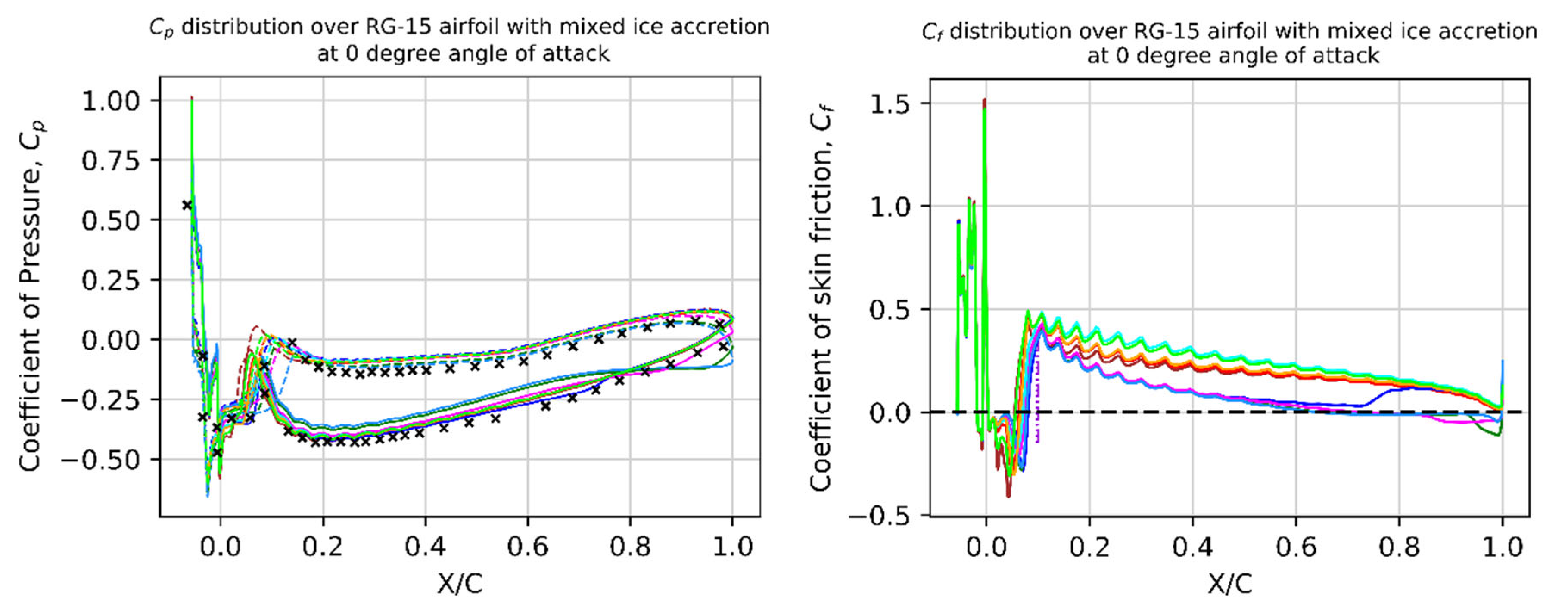
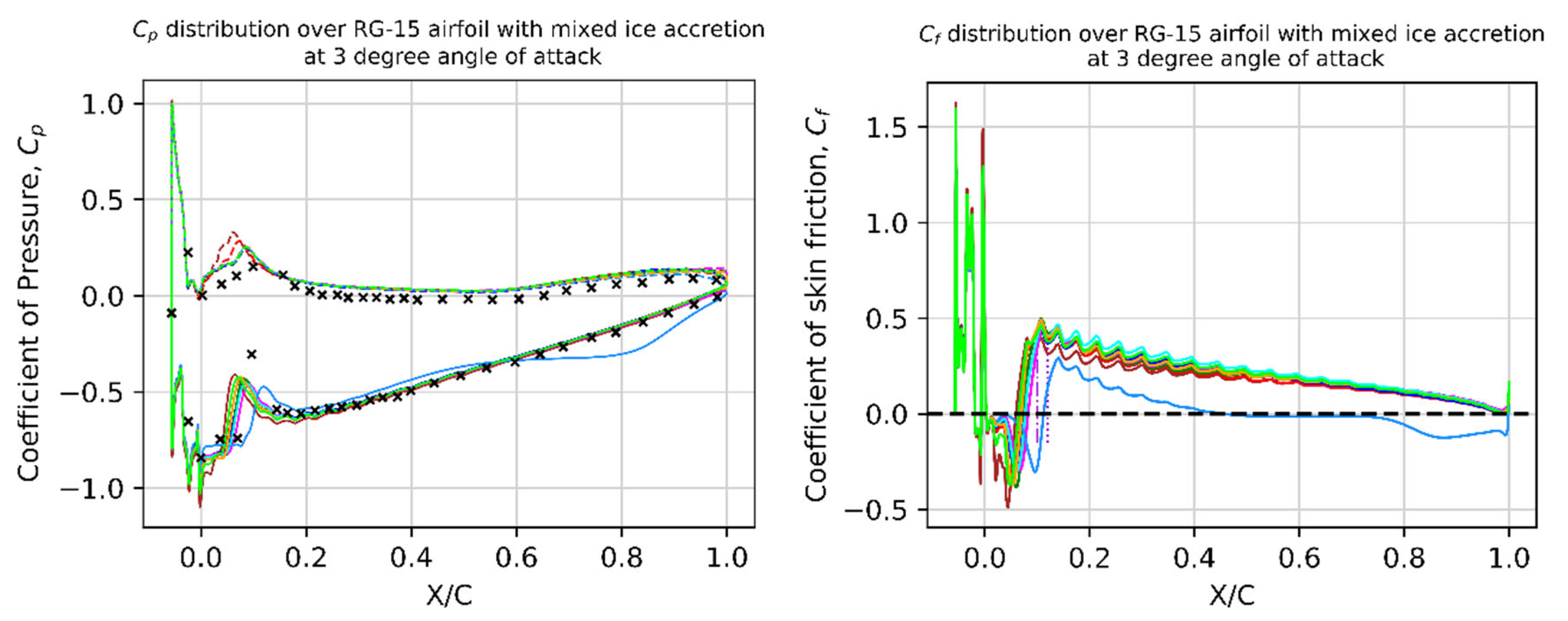
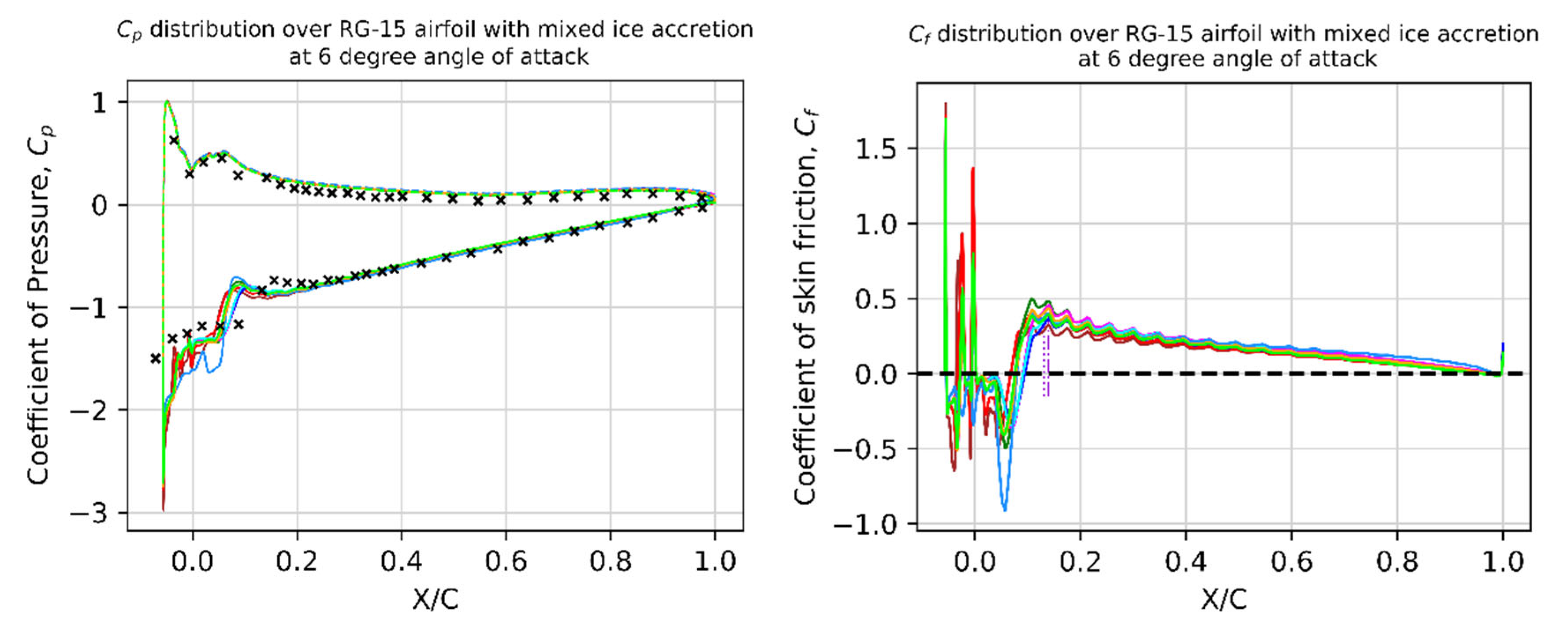
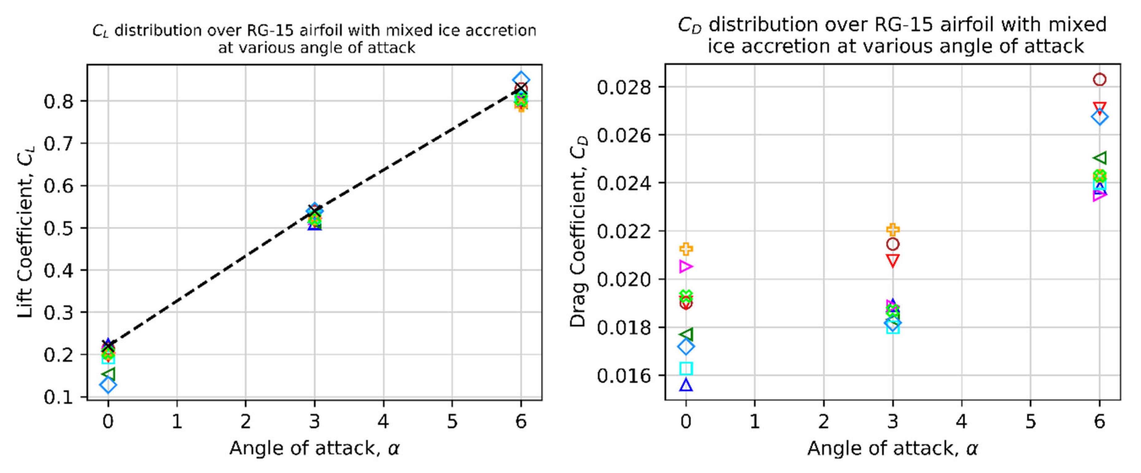
3.3. Ice-Induced Separation Bubbles (ISBs)

The nature of ISBs with an increase in the angle of attack on the surface of an RG-15 airfoil is shown in Figure 13. The point of onset of separation seems unaffected by the angle of attack as observed by previous researchers [6,24]. When the angle of attack increased from 3 degrees to 6 degrees, it can be observed from Figure 13 that a small, separated flow region exists ahead of the main separation bubble. Such separation bubbles are not reported in the experimental and LES studies, where the separation point remains the same for all angles of attack [24]. However, careful observation of the C f distribution and velocity contour presented by Oo et al. [6] reveals the existence of small separated flow regions aft of the main separation bubble. The separation and reattachment points are obtained from the C p plots as shown in Figure 14. Like LSBs, C p flattening and negative C f values are observed inside the separation bubble. Interestingly, it should be noted that, unlike LSBs, ISBs are observed on both the suction side and pressure side of the iced airfoil. However, the experimental data are only available for the ISBs formed on the suction side. For ISBs, the flow separation originates from the tip of the leading-edge ice horn as shown in Figure 2, so the reattachment location is the major focus when studying ISBs, in addition to the C p distribution. Further, the aerodynamic lift coefficients of the iced Rg-15 airfoil predicted by the numerical solvers are compared with the LES simulation data provided by Oo et al. [6]. It is important to note that the conventional RANS turbulence models are also quite capable of predicting ISBs, unlike LSBs. Figure 15 shows the C p distribution over the ISB region predicted by the K ω S S T model (representative of conventional RANS) and the γ R e θ transition model (representative of transition models). It can be observed that, unlike the LSB case, the experiments predicted a very distinct plateau in the region of ISBs. The conventional models are not able to predict a distinct plateau like the transition models. Also, the length of the plateau region increases with the angle of attack.

3.4. Fidelity of RANS Models in Predicting Ice Induced Separation Bubbles (ISBs)

In this section, the capability of various RANS turbulence models in predicting an ISB is studied. Oo et al. [6] in 2020 performed experimental and LES studies on an iced Rg-15 airfoil to study the behavior of ISBs. The C p distribution over an RG-15 airfoil with mixed ice accretion and the separation onset and reattachment location of ISB is reported in his work. The C p and C f distributions over the Rg-15 airfoil with mixed ice accretion at a 0-degree angle of attack for nine different RANS-based turbulence models are shown in Figure 16. The leading edge of the clean Rg-15 airfoil starts at X C = 0 and the region forward of this point represents the geometry of the ice. The onset of separation starts on the surface of the ice at X C = 0.0183 for all the turbulence models considered in this study, but the predictions of the reattachment location vary. Similar to the LSB case, the C p values are slightly overpredicted in the numerical studies, compared to experiments. Also, the values of the suction peak predicted by numerical simulations are quite high compared to experimental predictions. From Figure 15, it can be observed that the C p distribution in the ISB zone is well predicted by the transition models in comparison to the conventional models. However, from the C f distribution, it can be observed that the γ -based transition models and the K K l ω model predict a trailing edge separation bubble like LSB, which is not observed in experiments and LES simulation cases. Therefore, the C p values outside the ISB zone show deviations from experiments. From Table 2, it can be observed that the reattachment location predicted by the K ω S S T model with low R e correction gives the closest match to experiments, followed by the γ R e θ transition model.
For the 3-degree angle-of-attack case, except the K K l ω model, all other turbulence models predicted similar C p distributions outside the ISB zone as shown in Figure 17. This is because the K K l ω turbulence model predicts a long trailing edge separation bubble as evident from the C f distribution shown in Figure 17. On the pressure side, the C p values are slightly overpredicted by numerical simulations. Inside the ISB, the C p distribution does not match the experimental predictions well, but downstream of the bubble, the predictions perform quite well. The reattachment location predicted by the γ transition model is closer to the experimental prediction with a difference of 18% forward. The C p predictions are improved at a 6-degree angle of attack, except at regions inside the suction-side ISB as shown in Figure 18. An almost identical C p distribution is predicted by all the turbulence models considered in this study, except in regions inside the suction-side ISB. Likewise, the 0-degree case with the K ω S S T model with low R e correction has the closest prediction of the reattachment point compared to experiments. However, it should be noted that the deviation from experiments is considerably higher by 32%, as given in Table 2.
Figure 19 shows the numerical C L and C D values predicted by different turbulence models for the angles of attack considered in this study. The C L values are compared with the LES data available in the literature by Oo et al. [6]. The C D data from LES simulation were not available in the literature and are therefore not compared with tests. It should be noted that the SA turbulence model predicts C L much better than any other model considered in this study for all angles of attack. Such a conclusion about the effectiveness of the SA model was also made by Costes et al. [42] during his studies on the NACA 23,012 airfoil with spanwise ridge ice at a 2-degree angle of attack. Similar observations were also made by Fajt [74]. The geometry of ISBs may affect the drag coefficient more evidently than lift due to the increase in shear stress, and the lack of experimental/LES drag data is a hindrance to assessing the capability of these models in detail. The legend for Figure 16, Figure 17 and Figure 18 is given in Figure 20.
Figure 16. C p (left) and C f (right) distributions over Rg-15 airfoil with mixed ice at 0-degree AOA (See Figure 20 for legend).
Drones 08 00148 g016
Figure 17. C p (left) and C f (right) distribution over Rg-15 airfoil with mixed ice at 3-degree AOA (See Figure 20 for legend).
Drones 08 00148 g017
Figure 18. C p (left) and C f (right) distributions over Rg-15 airfoil with mixed ice at 6-degree AOA (See Figure 20 for legend).
Drones 08 00148 g018
Figure 19. C L (left) and C D (right) distributions over Rg-15 airfoil with mixed ice accretion (See Figure 20 for legend).
Drones 08 00148 g019
Figure 20. Legend for Figure 16, Figure 17, Figure 18 and Figure 19.
Drones 08 00148 g020
The RANS simulations underpredicted the reattachment location for all the angles of attack considered, and the growth of the separation bubble is limited to less than 15% as we increase the angle of attack from 0 to 6 degrees. However, the experimental studies predict 40% growth in the bubble length. Analogous observations were made by Bragg [24] during his experimental studies on the NACA 0012 airfoil as explained in Section 1.2. Thus, the RANS-based turbulence models predicted the reattachment much earlier than the actual scenario in the case of ISBs. This may be because the turbulence level predicted by the numerical solvers is higher than the experiments. These observations demand an improvement in the existing models for low-Reynolds-number ISB problems. Unlike LSBs, conventional turbulence is also capable of predicting ISBs, therefore the shear stress distribution does not vary considerably among the models except in cases where the use of transition models can lead to the prediction of nonphysical flow separation near the leading edge of the airfoil. Therefore, the low computational cost and simplicity associated with conventional RANS models make then a viable option to study ISBs with compromised accuracy.

4. Conclusions

The ability of nine distinct RANS-based turbulence models to predict the laminar separation bubble over the RG-15 airfoil at a Reynolds number of 1.07 × 10 5 was evaluated through comparison. Turbulence models with low Reynolds numbers that do not incorporate transition modeling are incapable of forecasting laminar separation bubbles; instead, they predict a fully attached flow at all angles of attack taken into account. Transition-based turbulence models are capable of predicting LSBs, but the predictions (location and size) differ among the models. Among the different transition models considered, the γ R e θ transition model has a better match with the experimental results for all of the angles of attack considered. The LSB migrates in the opposite direction of the flow as the angle of attack increases, while the separation bubble becomes smaller in both length and thickness. Conventional RANS-based models are also capable of predicting the ISB. Thus, unlike LSBs, the study of ISBs does not demand the use of any transition-based turbulence modes, while in some cases, the use of such models can lead to the prediction of nonphysical flow separation near the leading edge of the airfoil. The SA turbulence model can be considered the most favored turbulence model to study the aerodynamic coefficient of Iced airfoils but is not quite reliable enough to estimate the pressure distribution and bubble geometry. Also, the predictions of separation and reattachment locations by RANS models are subjected to uncertainty. Thus, the use of a single turbulence model that can be reliably used for the entire ice accretion simulation is difficult to select from the observations made in this study. Transition-based models can be used for the initial shots of the ice accretion simulation, but they need to be changed to conventional RANS models once an ISB forms. This helps save computational time and prevents the use of non-physical shear stress and heat flux values in the ice accretion calculations.

Author Contributions

Conceptualization, M.M. and M.S.V.; methodology, M.M.; investigation, M.M.; data curation, M.M.; writing—original draft preparation, M.M.; writing—review and editing, M.M.; supervision, M.S.V. All authors have read and agreed to the published version of the manuscript.

Funding

The work reported in this paper is supported by the UiT—The Arctic University of Norway (Project no-7400-72104) & nICE project of UiT & Research Council of Norway (Project no-324156).

Data Availability Statement

The data that support the findings of this study are available from the corresponding author upon reasonable request.

Conflicts of Interest

The authors declare no conflicts of interest.

Appendix A

Figure A1. Grid independence study.
Drones 08 00148 g0a1
Figure A2. Comparison of steady-state and time-averaged simulation C p (left) and C f (right) predictions.
Drones 08 00148 g0a2

References

  1. Oo, N.L.; Richards, P.; Sharma, R. Influence of an ice-induced separation bubble on the laminar separation bubble on an RG-15 airfoil at low Reynolds numbers. In Proceedings of the AIAA Aviation 2020 Forum, Virtual, 15–19 June 2020. [Google Scholar]
  2. Tani, I. Low-speed flows involving bubble separations. Prog. Aerosp. Sci. 1964, 5, 70–103. [Google Scholar] [CrossRef]
  3. BRAGG, M.; Khodadoust, A. Experimental measurements in a large separation bubble due to a simulated glaze ice shape. In Proceedings of the 26th Aerospace Sciences Meeting, Reno, NV, USA, 11–14 January 1988; p. 116. [Google Scholar]
  4. Muhammed, M.; Virk, M.S. Ice Accretion on Fixed-Wing Unmanned Aerial Vehicle—A Review Study. Drones 2022, 6, 86. [Google Scholar] [CrossRef]
  5. Muhammed, M.; Virk, M.S. Ice Accretion on Rotary-Wing Unmanned Aerial Vehicles—A Review Study. Aerospace 2023, 10, 261. [Google Scholar] [CrossRef]
  6. Oo, N.L.; Richards, P.J.; Sharma, R.N. Ice-Induced Separation Bubble on RG-15 Airfoil at Low Reynolds Number. AIAA J. 2020, 58, 5156–5167. [Google Scholar] [CrossRef]
  7. ANSYS. ANSYS FENSAP-ICE User Manual 18.2; ANSYS: Canonsburg, PA, USA, 2017. [Google Scholar]
  8. Marxen, O.; Rist, U. DNS and LES of the Transition Process in a Laminar Separation Bubble. In Proceedings of the Direct and Large-Eddy Simulation V; Springer: Dordrecht, The Netherlands, 2004; pp. 231–240. [Google Scholar]
  9. Loth, E. Numerical approaches for motion of dispersed particles, droplets and bubbles. Prog. Energy Combust. Sci. 2000, 26, 161–223. [Google Scholar] [CrossRef]
  10. Hain, R.; Kähler, C.; Radespiel, R. Dynamics of laminar separation bubbles at low-Reynolds-number aerofoils. J. Fluid Mech. 2009, 630, 129–153. [Google Scholar] [CrossRef]
  11. Jones, B.M. Stalling. Aeronaut. J. 1934, 38, 753–770. [Google Scholar] [CrossRef]
  12. Horton, H.; Young, A. Some results of investigations of separation bubbles (Flow separation bubble data, and comparisons with velocity and pressure measurements). AGARD CP 1966, 779–811. [Google Scholar]
  13. Horton, H.P. Laminar Separation Bubbles in Two and Three Dimensional Incompressible Flow. Ph.D. Thesis, Queen Mary University of London, London, UK, 1968. [Google Scholar]
  14. Choudhry, A.; Arjomandi, M.; Kelso, R. A Study of Long Separation Bubble on Thick Airfoils and Its Consequent Effects. Int. J. Heat Fluid Flow 2015, 52, 84–96. [Google Scholar] [CrossRef]
  15. Gray, V.H. Aerodynamic Effects Caused by Icing of an Unswept NACA 65A004 Airfoil; National Advisory Committee for Aeronautics: Washington, DC, USA; Lewis Flight Propulsion Lab: Washington, DC, USA, 1958. [Google Scholar]
  16. Kim, H.; Bragg, M. Effects of leading-edge ice accretion geometry on airfoil performance. In Proceedings of the 17th Applied Aerodynamics Conference, Norfolk, VA, USA, 28 June–1 July 1999. [Google Scholar]
  17. Lee, S.; Bragg, M.B. Experimental Investigation of Simulated Large-Droplet Ice Shapes on Airfoil Aerodynamics. J. Aircr. 1999, 36, 844–850. [Google Scholar] [CrossRef]
  18. Lee, S.; Bragg, M.B. Investigation of Factors Affecting Iced-Airfoil Aerodynamics. J. Aircr. 2003, 40, 499–508. [Google Scholar] [CrossRef]
  19. Lee, S.; Kim, H.; Bragg, M. Investigation of factors that influence iced-airfoil aerodynamics. In Proceedings of the 38th Aerospace Sciences Meeting and Exhibit, Reno, NV, USA, 10–13 January 2000; American Institute of Aeronautics and Astronautics: Reston, VA, USA, 2000. [Google Scholar]
  20. Bragg, M. Predicting Airfoil Performance with Rime and Glaze Ice Accretions. In Proceedings of the AIAA 22nd Aerospace Sciences Meeting, Reno, Nevada, January 1984; Paper No. AIAA-84-0106. [Google Scholar]
  21. Bragg, M.; Coirier, W. Aerodynamic measurements of an airfoil with simulated glaze ice. In Proceedings of the 24th Aerospace Sciences Meeting, Reno, NV, USA, 6–9 January 1986. [Google Scholar]
  22. Bragg, M.; Gregorek, G.; Shaw, R. Wind tunnel investigation of airfoil performance degradation due to icing. In Proceedings of the AIAA 12th Aerodynamic Testing Conference, Williamsburg, VA, USA, 22–24 March 1982. Paper No. AIAA-82-0582. [Google Scholar]
  23. Bragg, M.B. Experimental aerodynamic characteristics of an NACA 0012 airfoil with simulated glaze ice. J. Aircr. 1988, 25, 849–854. [Google Scholar] [CrossRef]
  24. Bragg, M.B.; Khodadoust, A.; Spring, S.A. Measurements in a leading-edge separation bubble due to a simulated airfoil ice accretion. AIAA J. 1992, 30, 1462–1467. [Google Scholar] [CrossRef]
  25. Bragg, M.B.; Zaguli, R.; Gregorek, G. Wind Tunnel Evaluation of Air-Foil Performance Using Simulated Ice Shapes; No.NAS 1.26:167960; NASA-CR-167960; NASA Center for AeroSpace Information (CASI): Hanover, MD, USA, 1982. [Google Scholar]
  26. Bragg, M.; Coirier, W. Detailed measurements of the flowfield in the vicinity of an airfoilwith glaze ice. In Proceedings of the 23rd Aerospace Sciences Meeting, Reno, NV, USA, 14–17 January 1985. [Google Scholar]
  27. Gurbacki, H.; Bragg, M. Unsteady aerodynamic measurements on an iced airfoil. In Proceedings of the 40th AIAA Aerospace Sciences Meeting & Exhibit, Reno, NV, USA, 14–17 January 2002. [Google Scholar]
  28. Bragg, M.B.; Broeren, A.P.; Blumenthal, L.A. Iced-airfoil aerodynamics. Prog. Aerosp. Sci. 2005, 41, 323–362. [Google Scholar] [CrossRef]
  29. Stebbins, S.J.; Loth, E.; Broeren, A.P.; Potapczuk, M. Review of computational methods for aerodynamic analysis of iced lifting surfaces. Prog. Aerosp. Sci. 2019, 111, 100583. [Google Scholar] [CrossRef]
  30. Kwon, O.; Sankar, L. Numerical study of the effects of icing on finite wing aerodynamics. In Proceedings of the 28th Aerospace Sciences Meeting, Reno, NV, USA, 8–11 January 1990. [Google Scholar]
  31. Kwon, O.J.; Sankar, L.N. Numerical simulation of the flow about a swept wing with leading-edge ice accretions. Comput. Fluids 1997, 26, 183–192. [Google Scholar] [CrossRef]
  32. Potapczuk, M.; Bragg, M.; Kwon, O.; Sankar, L. Simulation of iced wing aerodynamics. In Proceedings of the Fluid Dynamics Panel Specialists Meeting, Toulouse, France, 29 April–1 May 1991. [Google Scholar]
  33. Alam, M.F.; Thompson, D.S.; Walters, D.K. Hybrid Reynolds-Averaged Navier–Stokes/Large-Eddy Simulation Models for Flow Around an Iced Wing. J. Aircr. 2015, 52, 244–256. [Google Scholar] [CrossRef]
  34. Mogili, P.; Thompson, D.; Choo, Y.; Addy, H. RANS and DES Computations for a Wing with Ice Accretion. In Proceedings of the 43rd AIAA Aerospace Sciences Meeting and Exhibit, Reno, NV, USA, 10–13 January 2005. [Google Scholar]
  35. Jun, G.; Oliden, D.; Potapczuk, M.G.; Tsao, J.-C. Computational Aerodynamic Analysis of Three-dimensional Ice Shapes on a NACA 23012 Airfoil. In Proceedings of the 6th AIAA Atmospheric and Space Environments Conference, Atlanta, GA, USA, 16–20 June 2014. [Google Scholar]
  36. Chi, K.; Williams, B.; Kreeger, R.; Hindman, R.; Shih, T. Simulations of Finite Wings with 2-D and 3-D Ice Shapes: Modern Lifting-Line Theory Versus 3-D CFD. In Proceedings of the 45th AIAA Aerospace Sciences Meeting and Exhibit, Reno, NV, USA, 8–11 January 2007. [Google Scholar]
  37. Chi, X.; Williams, B.; Crist, N.; Kreeger, R.; Hindman, R.; Shih, T. 2-D and 3-D CFD Simulations of a Clean and an Iced Wing. In Proceedings of the 44th AIAA Aerospace Sciences Meeting and Exhibit, Reno, NV, USA, 9–12 January 2006. [Google Scholar]
  38. Khalid, M.; Zhang, F. The aerodynamic studies of aircraft wings with leading edge deformations due to accreted ice. In Proceedings of the 40th AIAA Aerospace Sciences Meeting & Exhibit, Reno, NV, USA, 14–17 January 2002. [Google Scholar]
  39. Oztekin, E.S.; Riley, J.T. Ice accretion on a NACA 23012 airfoil. In Proceedings of the 2018 Atmospheric and Space Environments Conference, Atlanta, GA, USA, 25–29 June 2018; American Institute of Aeronautics and Astronautics: Reston, VA, USA, 2018. [Google Scholar]
  40. Thompson, D.; Mogili, P.; Chalasani, S.; Addy, H.; Choo, Y. A Computational Icing Effects Study for a Three-Dimensional Wing. In Proceedings of the 42nd AIAA Aerospace Sciences Meeting and Exhibit, Reno, NV, USA, 5–8 January 2004; American Institute of Aeronautics and Astronautics: Reston, VA, USA, 2004. [Google Scholar]
  41. Costes, M.; Moens, F. Advanced numerical prediction of iced airfoil aerodynamics. Aerosp. Sci. Technol. 2019, 91, 186–207. [Google Scholar] [CrossRef]
  42. Costes, M.; Moens, F.; Brunet, V. Prediction of iced airfoil aerodynamic characteristics. In Proceedings of the 54th AIAA Aerospace Sciences Meeting, San Diego, CA, USA, 4–8 January 2016. [Google Scholar]
  43. Papadakis, M.; Strong, P.; Wong, J.; Wong, S. Simulation of Residual and Intercycle Ice Shapes Using Step Ice and Roughness. In Proceedings of the 4th AIAA Atmospheric and Space Environments Conference, New Orleans, LA, USA, 25–28 June 2012; American Institute of Aeronautics and Astronautics: Reston, VA, USA, 2012. [Google Scholar]
  44. Menter, F.; Esch, T.; Kubacki, S. Transition modelling based on local variables. In Engineering Turbulence Modelling and Experiments 5; Elsevier: Amsterdam, The Netherlands, 2002; pp. 555–564. [Google Scholar]
  45. Van Ingen, J. A Suggested Semi-Empirical Method for the Calculation of the Boundary Layer Transition Region; Report V.T.H.-74; Technische Hogeschool Delft, Vliegtuigbouwkunde: Delft, The Netherlands, 1956. [Google Scholar]
  46. Smith, A.M.O. Transition, Pressure Gradient and Stability Theory; Report ES 26388; Douglas Aircraft Company: Santa Monica, CA, USA, 1956. [Google Scholar]
  47. Jones, W.P.; Launder, B.E. The prediction of laminarization with a two-equation model of turbulence. Int. J. Heat Mass Transf. 1972, 15, 301–314. [Google Scholar] [CrossRef]
  48. Hadzic, I. Second-Moment Closure Modelling of Transitional and Unsteady Turbulent Flows. Ph.D. Thesis, Delft University of Technology (TU Delft), Delft, The Netherlands, 1999. Available online: http://resolver.tudelft.nl/uuid:f39d1a49-a9e8-4c32-beb6-02fd2358d3ac (accessed on 12 November 2023).
  49. Priddin, C.H. Behaviour of the Turbulent Boundary Layer on Curved, Porous Walls. Ph.D. Thesis, Imperial College, London, UK, 1974. Available online: https://ntrs.nasa.gov/api/citations/19880013801/downloads/19880013801.pdf (accessed on 12 November 2023).
  50. Rodi, W.; Scheuerer, G. Calculation of laminar-turbulent boundary layer transition on turbine blades. In AGARD Heat Tranfer and Cooling in Gas Turbines; Advisory Group for Aerospace Research and Development (AGARD): Brussels, Belgium, 1985. [Google Scholar]
  51. Hallbäck, M.; Henningson, D.; Johansson, A.; Alfredsson, P. Turbulence and Transition Modelling: Lecture Notes from the ERCOFTAC/IUTAM Summerschool, Proceedings of the ERCOFTAC/IUTAM Summerschool, Stockholm, Sweden, 12–20 June 1995; Springer Science & Business Media: New York, NY, USA, 1996; Volume 2. [Google Scholar]
  52. Dhawan, S.; Narasimha, R. Some properties of boundary layer flow during the transition from laminar to turbulent motion. J. Fluid Mech. 1958, 3, 418–436. [Google Scholar] [CrossRef]
  53. Abu-Ghannam, B.J.; Shaw, R. Natural Transition of Boundary Layers—The Effects of Turbulence, Pressure Gradient, and Flow History. J. Mech. Eng. Sci. 1980, 22, 213–228. [Google Scholar] [CrossRef]
  54. Mayle, R.E. The Role of Laminar-Turbulent Transition in Gas Turbine Engines. In Proceedings of the ASME 1991 International Gas Turbine and Aeroengine Congress and Exposition, Orlando, FL, USA, 3–6 June 1991; American Society of Mechanical Engineers (ASME): New York, NY, USA, 1961; Volume 5. V005T17A001. [Google Scholar] [CrossRef]
  55. Gostelow, J.P.; Blunden, A.R.; Walker, G.J. Effects of Free-Stream Turbulence and Adverse Pressure Gradients on Boundary Layer Transition. J. Turbomach. 1994, 116, 392–404. [Google Scholar] [CrossRef]
  56. Steelant, J.; Dick, E. Modelling of bypass transition with conditioned Navier-Stokes equations coupled to an intermittency transport equation. Int. J. Numer. Methods Fluids 1996, 23, 193–220. [Google Scholar] [CrossRef]
  57. Cho, J.R.; Chung, M.K. AK—ε—γ equation turbulence model. J. Fluid Mech. 1992, 237, 301–322. [Google Scholar] [CrossRef]
  58. Suzen, Y.; Huang, P. An intermittency transport equation for modeling flow transition. In Proceedings of the 38th Aerospace Sciences Meeting and Exhibit, Reston, VA, USA, 10–13 January 2000. [Google Scholar]
  59. Menter, F.R.; Langtry, R.B.; Likki, S.; Suzen, Y.; Huang, P.; Völker, S. A correlation-based transition model using local variables—Part I: Model formulation. J. Turbomach. 2006, 12, 413–422. [Google Scholar] [CrossRef]
  60. Spalart, P.; Allmaras, S. A One-Equation Turbulence Model for Aerodynamic Flows; AIAA: Reston, VA, USA, 1992; p. 439. [Google Scholar]
  61. Menter, F.R. Two-equation eddy-viscosity turbulence models for engineering applications. AIAA J. 1994, 32, 1598–1605. [Google Scholar] [CrossRef]
  62. Launder, B.E.; Spalding, D.B. Lectures in Mathematical Models of Turbulence; Academic Press: Cambridge, MA, USA, 1972. [Google Scholar]
  63. Ansys Inc. Ansys Fluent Theory Guide; Ansys Inc.: Canonsburg, PA, USA, 2022. [Google Scholar]
  64. Suzen, Y.B.; Huang, P.G. Modeling of Flow Transition Using an Intermittency Transport Equation. J. Fluids Eng. 2000, 122, 273–284. [Google Scholar] [CrossRef]
  65. Langtry, R.B.; Menter, F. Correlation-Based Transition Modeling for Unstructured Parallelized Computational Fluid Dynamics Codes. AIAA J. 2009, 47, 2894–2906. [Google Scholar] [CrossRef]
  66. Walters, D.K.; Cokljat, D. A three-equation eddy-viscosity model for Reynolds-averaged Navier–Stokes simulations of transitional flow. J. Fluids Eng. 2008, 130, 121401. [Google Scholar] [CrossRef]
  67. Williams, N.; Benmeddour, A.; Brian, G.; Ol, M. The effect of icing on small unmanned aircraft low Reynolds number airfoils. In Proceedings of the 17th Australian International Aerospace Congress (AIAC), Melbourne, Australia, 26–28 February 2017. [Google Scholar]
  68. Muhammed, M.; Virk, M. Steady and Time Dependent Study of Laminar Separation Bubble (LSB) behavior along UAV Airfoil RG-15. Int. J. Multiphys. 2023, 17, 55–76. [Google Scholar]
  69. Lee, C.-S.; Pang, W.; Srigrarom, S.; Wang, D.B.; Hsiao, F.-B. Classification of airfoils by abnormal behavior of lift curves at low Reynolds number. In Proceedings of the 24th AIAA Applied Aerodynamics Conference, San Francisco, CA, USA, 5–8 June 2006; Volume 2. [Google Scholar]
  70. Miozzi, M.; Capone, A.; Costantini, M.; Fratto, L.; Klein, C.; Di Felice, F. Skin friction and coherent structures within a laminar separation bubble. Exp. Fluids 2018, 60, 13. [Google Scholar] [CrossRef]
  71. Zhang, K.; Rival, D.E. Direct Lagrangian method to characterize entrainment dynamics using particle residence time: A case study on a laminar separation bubble. Exp. Fluids 2020, 61, 243. [Google Scholar] [CrossRef]
  72. Swift, K.M. An Experimental Analysis of the Laminar Separation Bubble at Low Reynolds Numbers. Master’s Thesis, University of Tennessee, Knoxville, TN, USA, 2009. [Google Scholar]
  73. Selig, M.S. Summary of Low Speed Airfoil Data; SoarTech Publications: Champaign, IL, USA, 1995. [Google Scholar]
  74. Fajt, N.; Hann, R.; Lutz, T. The Influence of Meteorological Conditions on the Icing Performance Penalties on a UAV Airfoil. In Proceedings of the 8th European Conference for Aeronautics and Space Sciences (EUCASS), Madrid, Spain, 1–4 July 2019. [Google Scholar]
Figure 1. Fundamental structure of LSB [14].
Drones 08 00148 g001
Figure 2. ISB on the suction surface of an ice accreted NACA 0012 [28].
Drones 08 00148 g002
Figure 3. Computational mesh over RG-15 Airfoil.
Drones 08 00148 g003
Figure 4. Velocity contours showing LSB on Rg15 airfoil at (a) 0-deg (top), (b) 3-deg (middle), and (c) 6-deg (bottom) angles of attack (predictions by γ R e θ transition turbulence models).
Drones 08 00148 g004
Figure 5. Determination of separation and reattachment location of LSB from   C p distribution [28].
Drones 08 00148 g005
Figure 6. C p (green) distribution and C f (red) distribution over Rg-15 airfoil at 6-degree angle of attack; the predicted LSB is shown at the bottom in red with the velocity vector in cyan color ( γ R e θ transition model).
Drones 08 00148 g006
Figure 7. Velocity profiles at specific X/C locations.
Drones 08 00148 g007
Figure 13. Velocity contours showing ISB on Rg15 airfoil at (a) 0-deg (top), (b) 3-deg (middle), and (c) 6-deg (bottom) angles of attack (predictions by SA turbulence model).
Drones 08 00148 g013
Figure 14. Determination of separation and reattachment locations of ISBs from C p distribution [28].
Drones 08 00148 g014
Figure 15. Comparison of C p predictions of K ω S S T (red) and transition K ω S S T (green) models (a) 0 deg, (b) 3 deg and (c) 6 deg.
Drones 08 00148 g015
Table 1. Separation and reattachment locations of LSBs on the surface of Rg-15 airfoil.
AOA0 Deg% Diff from Exp% Diff from LES3 Deg% Diff from Exp% Diff from LES6 Deg% Diff from Exp% Diff from LES
Turbulence ModelSeperationSeperationSeperationSeperationReattachmentSeperationReattachmentSeperationReattachmentSeperationReattachmentSeperationReattachmentSeperationReattachment
Experiments0.780.0011.110.540.880.000.00−1.100.000.240.490.000.0022.4511.36
LES0.70−10.000.000.550.881.110.000.000.000.200.44−18.33−10.200.000.00
SA---------------
K-W---------------
low re KW---------0.200.37−16.67−23.672.04−15.00
Trans KW0.73−6.413.990.530.87−1.85−0.68−2.93−0.680.200.46−16.67−6.732.043.86
gamma0.69−11.54−1.710.511.00−5.5613.64−6.5913.640.190.47−21.25−4.69−3.576.14
lowre gamma0.65−16.67−7.410.511.00−5.5613.64−6.5913.640.180.47−25.00−4.49−8.166.36
k-kl-w0.68−12.82−3.130.471.00−12.9613.64−13.9213.640.160.50−33.332.86−18.3714.55
algebraic0.75−3.856.840.550.781.85−11.020.73−11.020.200.40−16.67−19.182.04−10.00
low re algebraic0.77−1.289.690.481.00−11.1113.64−12.0913.640.190.47−20.83−4.69−3.066.14
Table 2. Separation and reattachment locations of ISBs on the surface of Rg-15 airfoil.
AOA0 Deg 3 Deg 6 Deg
Turbulence ModelSeperationReattachment% Diff from Exp% Diff from LESSeperationReattachment% Diff from Exp% Diff from LESSeperationReattachment% Diff from Exp% Diff from LES
Experiments0.000.100.003.090.000.100.00−15.970.000.140.006.92
LES0.000.10−3.000.000.000.1219.000.000.000.13−6.470.00
SA−0.020.05−46.00−44.33−0.020.06−41.00−50.42−0.050.07−51.44−48.08
K-W−0.020.06−37.50−35.57−0.020.07−30.50−41.60−0.050.07−51.44−48.08
low re KW−0.020.08−20.00−17.53−0.020.08−25.00−36.97−0.050.09−32.37−27.69
Trans KW−0.020.08−22.50−20.10−0.020.08−25.00−36.97−0.050.08−45.32−41.54
gamma−0.020.07−27.00−24.74−0.020.08−18.00−31.09−0.050.09−35.25−30.77
lowre gamma−0.020.07−30.00−27.84−0.020.08−23.00−35.29−0.050.09−34.53−30.00
k-kl-w−0.020.08−23.00−20.62−0.020.1112.00−5.88−0.050.08−43.17−39.23
algebraic−0.020.07−35.00−32.99−0.020.07−30.50−41.60−0.050.08−43.88−40.00
low re algebraic−0.020.06−44.50−42.78−0.020.06−35.60−45.88−0.050.08−45.68−41.92
Disclaimer/Publisher’s Note: The statements, opinions and data contained in all publications are solely those of the individual author(s) and contributor(s) and not of MDPI and/or the editor(s). MDPI and/or the editor(s) disclaim responsibility for any injury to people or property resulting from any ideas, methods, instructions or products referred to in the content.

