

Aerodynamic Interaction Minimization in Coaxial Multirotors via Optimized Control Allocation


Abstract
:1. Introduction
1.1. Related Work
1.2. Contributions
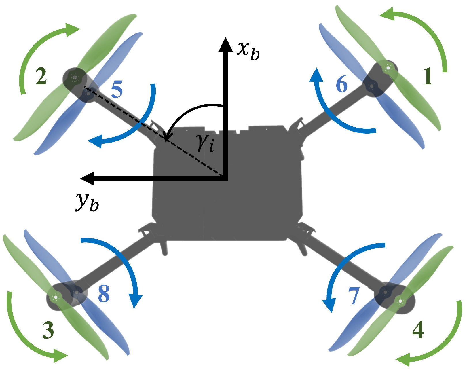
2. Coaxial Rotor
2.1. Model
2.2. Identification Method
3. Coaxial Rotor Experiments and Analysis
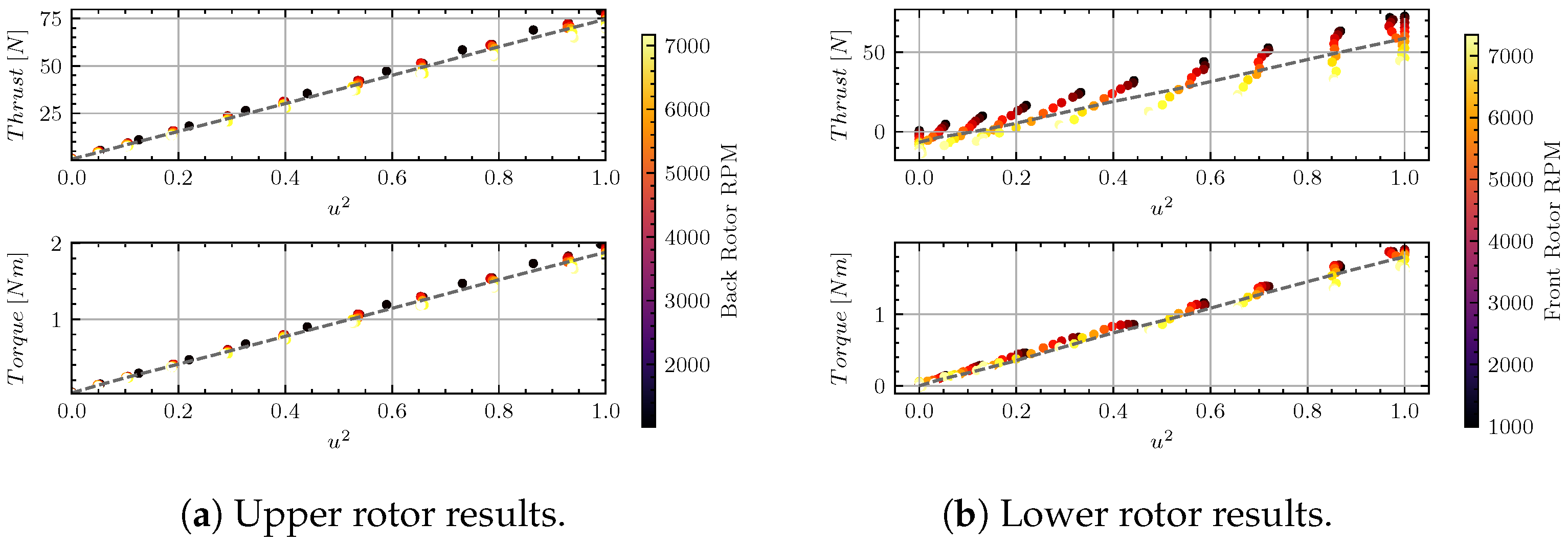
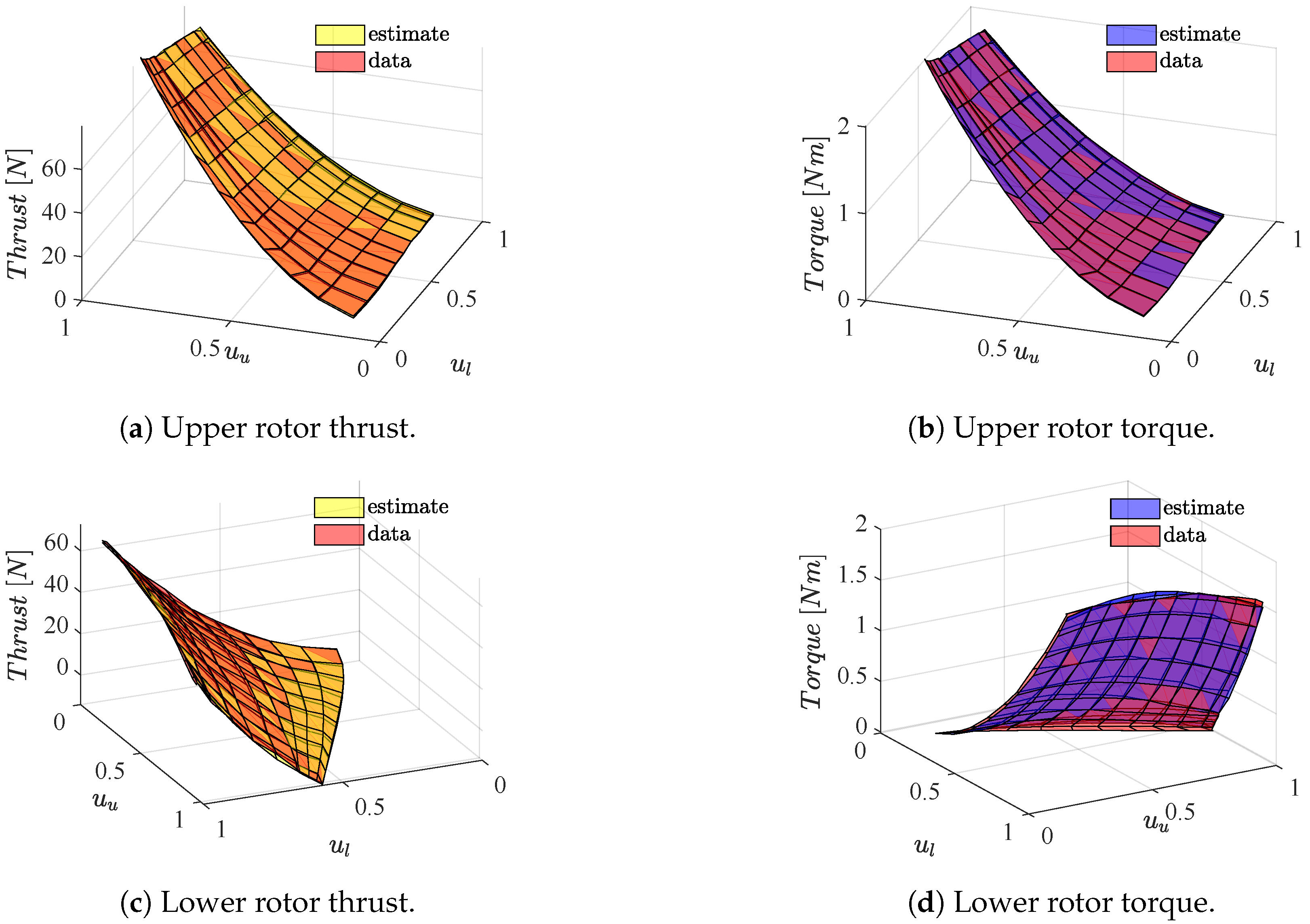
3.1. Parameter Identification
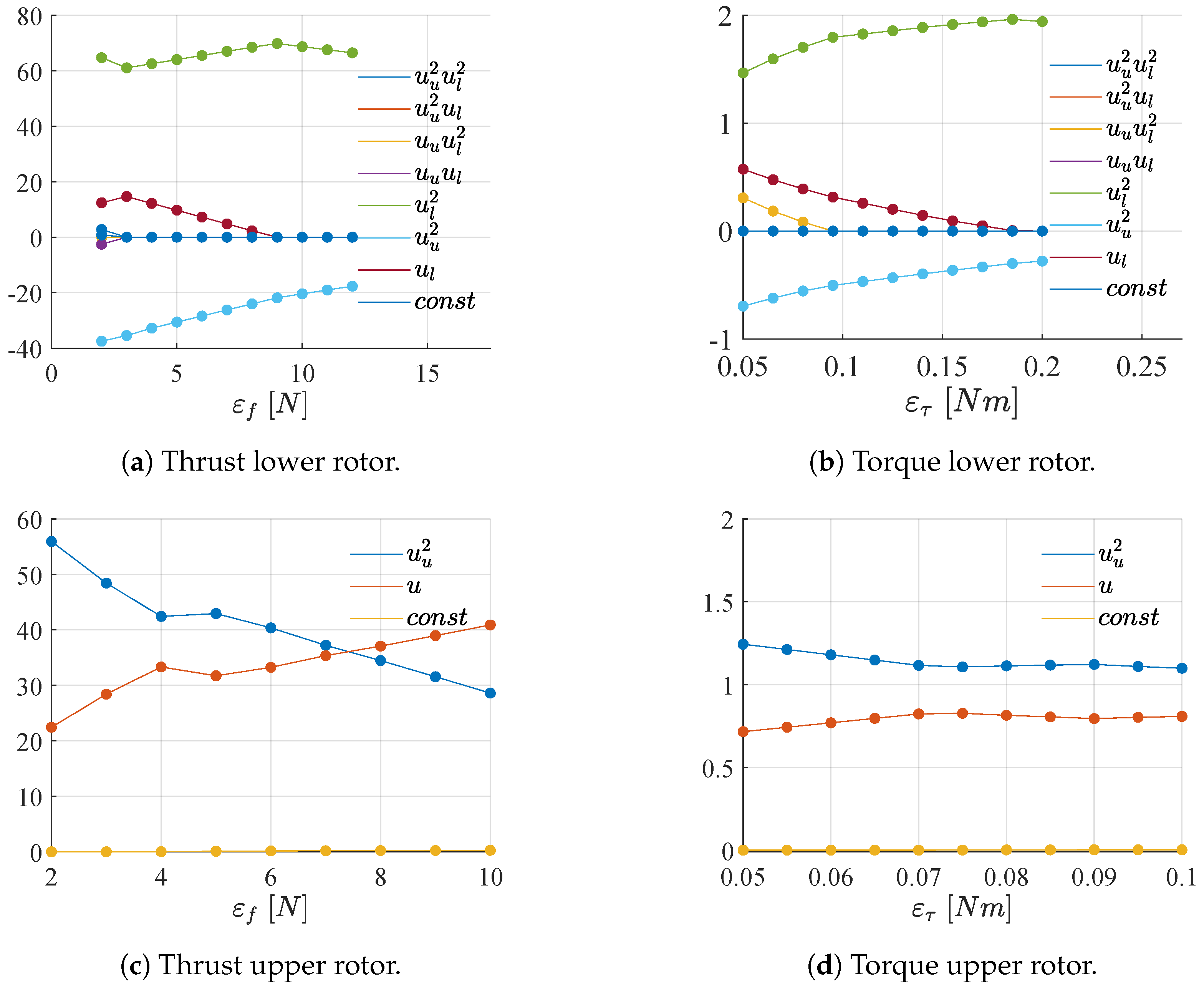
3.2. Tolerance Analysis
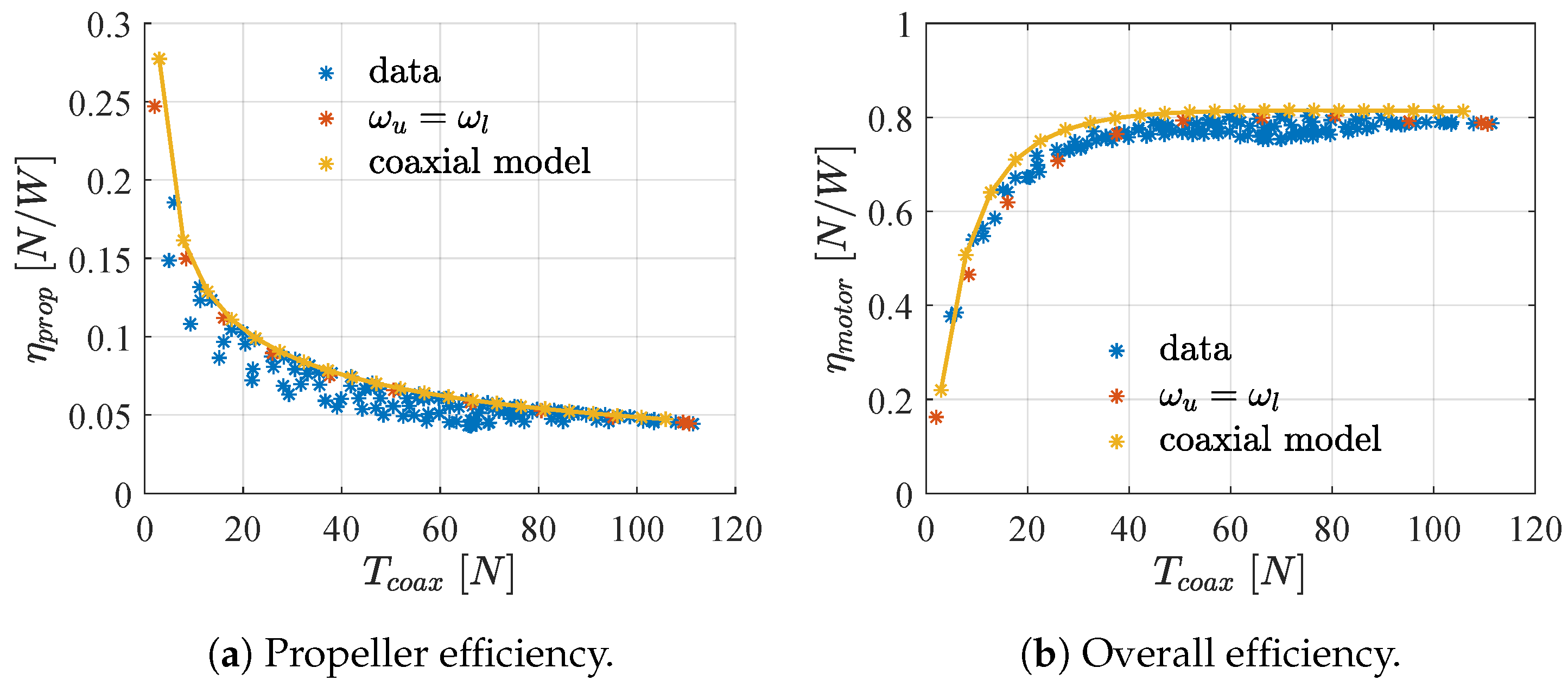
3.3. Efficiency
4. Coaxial Control Allocation Strategies
4.1. Reduced Coaxial Mixer
4.2. Coaxial Mixer
| Algorithm 1 Coaxial Control Allocation algorithm |
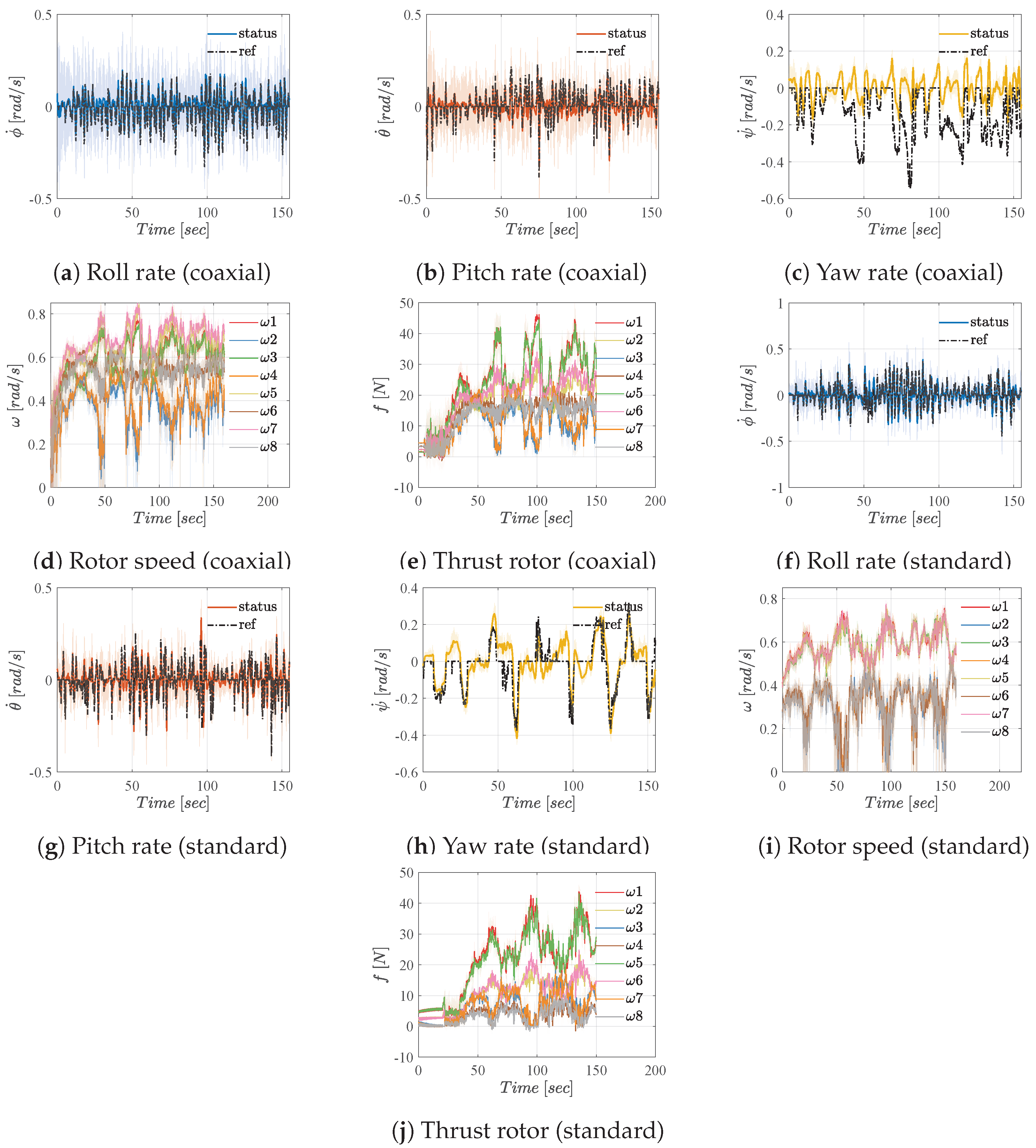
5. Control Allocation Experiments
5.1. Experimental Setup
5.2. Control Allocation Implementation
5.2.1. Reduced Coaxial Mixer
5.2.2. Coaxial Mixer
5.2.3. Standard Mixer
5.3. Software-In-The-Loop
5.4. Flight Test
6. Conclusions
- Incorporating aerodynamic interactions into lower rotor models results in a reduction of both thrust and torque errors compared to standard models, with a decrease in thrust error of approximately 12 N and a reduction in total torque error of about 0.043 Nm.
- Adoption of a LASSO-based technique as the identification method for model parameters prevents model overfitting and decreases initial model complexity, thereby improving computational efficiency, with the price of lower accuracy, but still a better one with respect to state-of-the-art solutions. Relaxation of LASSO tolerance results in a further reduction in model complexity, resulting in a quadratic model.
- Two coaxial mixer strategies were implemented based on coaxial rotor models: Coaxial Mixer and Reduced-Coaxial Mixer. The Coaxial Mixer utilizes the pseudo-inversion of a static control allocation matrix, while for Reduced-Coaxial Mixer rotor velocities are derived from the solution of second-order equations. Both mixers improve thrust tracking accuracy and rotor efficiency compared to standard mixer solutions. Specifically:
- −
- Coaxial Mixer generates the minimum thrust and position errors but results in increased attitude error compared to the Reduced-Coaxial Mixer.
- −
- Reduced-Coaxial Mixer achieves better attitude and torque tracking but larger thrust and position errors with respect to the previous one.
Author Contributions
Funding
Data Availability Statement
Conflicts of Interest
References
- Hamandi, M.; Usai, F.; Sablé, Q.; Staub, N.; Tognon, M.; Franchi, A. Design of multirotor aerial vehicles: A taxonomy based on input allocation. Int. J. Robot. Res. 2021, 40, 1015–1044. [Google Scholar] [CrossRef]
- Haddadi, S.J.; Zarafshan, P.; Dehghani, M. A coaxial quadrotor flying robot: Design, analysis and control implementation. Aerosp. Sci. Technol. 2022, 120, 107260. [Google Scholar] [CrossRef]
- Hosseini, S.; Rhein, J.; Sax, F.; Hofsäß, H.; Holzapfel, F.; Maier, L.; Barth, A.; Grebing, B. Conversion of a Coaxial Rotorcraft to a UAV. In Proceedings of the AIAA SciTech 2024 Forum, Orlando, FL, USA, 8–12 January 2024; p. 1716. [Google Scholar]
- Marredo, J.; Petrus, A.; Trujillo, M.; Viguria, A.; Ollero, A. A Novel Unmanned Aerial System for Power Line Inspection and Maintenance Operations. In Proceedings of the 2024 International Conference on Unmanned Aircraft Systems (ICUAS), Chania, Greece, 4–7 June 2024; IEEE: Piscataway, NJ, USA, 2024; pp. 602–609. [Google Scholar]
- Johansen, T.A.; Fossen, T.I. Control allocation—A survey. Automatica 2013, 49, 1087–1103. [Google Scholar] [CrossRef]
- Monteiro, J.C.; Lizarralde, F.; Hsu, L. Optimal control allocation of quadrotor UAVs subject to actuator constraints. In Proceedings of the 2016 American Control Conference (ACC), Boston, MA, USA, 6–8 July 2016; IEEE: Piscataway, NJ, USA, 2016; pp. 500–505. [Google Scholar]
- Faessler, M.; Falanga, D.; Scaramuzza, D. Thrust mixing, saturation, and body-rate control for accurate aggressive quadrotor flight. IEEE Robot. Autom. Lett. 2016, 2, 476–482. [Google Scholar] [CrossRef]
- Johansen, T.A.; Fossen, T.I.; Berge, S.P. Constrained nonlinear control allocation with singularity avoidance using sequential quadratic programming. IEEE Trans. Control. Syst. Technol. 2004, 12, 211–216. [Google Scholar] [CrossRef]
- Bezerra, J.A.; Santos, D.A. Optimal exact control allocation for under-actuated multirotor aerial vehicles. IEEE Control Syst. Lett. 2021, 6, 1448–1453. [Google Scholar] [CrossRef]
- Madruga, S.P.; Tavares, A.H.; Luiz, S.O.; do Nascimento, T.P.; Lima, A.M.N. Aerodynamic effects compensation on multi-rotor UAVs based on a neural network control allocation approach. IEEE/CAA J. Autom. Sin. 2021, 9, 295–312. [Google Scholar] [CrossRef]
- McCormick, B.W. Aerodynamics, Aeronautics, and Flight Mechanics; John Wiley & Sons: Hoboken, NJ, USA, 1994. [Google Scholar]
- Coleman, C.P. A Survey of Theoretical and Experimental Coaxial Rotor Aerodynamic Research; Technical Report; NASA: Washington, DC, USA, 1997. [Google Scholar]
- Yoon, S.; Chan, W.M.; Pulliam, T.H. Computations of torque-balanced coaxial rotor flows. In Proceedings of the 55th AIAA Aerospace Sciences Meeting, Grapevine, TX, USA, 9–13 January 2017; p. 0052. [Google Scholar]
- Park, S.H.; Kwon, O.J. Numerical study about aerodynamic interaction for coaxial rotor blades. Int. J. Aeronaut. Space Sci. 2021, 22, 277–286. [Google Scholar] [CrossRef]
- Lei, Y.; Wang, J.; Yang, W. Aerodynamic Performance of a Coaxial Hex-Rotor MAV in Hover. Aerospace 2021, 8, 378. [Google Scholar] [CrossRef]
- Khan, H.Z.I.; Mobeen, S.; Rajput, J.; Riaz, J. Nonlinear control allocation: A learning based approach. arXiv 2022, arXiv:2201.06180. [Google Scholar]
- Spaans, J.; Gilbert, S.; Stol, K.A.; Al-Zubaidi, S. System Identification for Fully-Actuated UAV Control Allocation. In Proceedings of the 2024 International Conference on Unmanned Aircraft Systems (ICUAS), Nanchang, China, 20–22 September 2024; IEEE: Piscataway, NJ, USA, 2024; pp. 193–200. [Google Scholar]
- Malakouti Khah, M.; Esmailifar, S.M.; Saadat, S. Design and development of a novel multirotor configuration with counter-rotating coaxial propellers. Sci. Rep. 2024, 14, 11580. [Google Scholar] [CrossRef] [PubMed]
- Bodie, K.; Taylor, Z.; Kamel, M.; Siegwart, R. Towards efficient full pose omnidirectionality with overactuated mavs. In Proceedings of the 2018 International Symposium on Experimental Robotics, Buenos Aires, Argentina, 5–8 November 2018; Springer: Berlin/Heidelberg, Germany, 2020; pp. 85–95. [Google Scholar]
- Dominguez, V.H.; Garcia-Salazar, O.; Amezquita-Brooks, L.; Reyes-Osorio, L.A.; Santana-Delgado, C.; Rojo-Rodriguez, E.G. Micro coaxial drone: Flight dynamics, simulation and ground testing. Aerospace 2022, 9, 245. [Google Scholar] [CrossRef]
- Koehl, A.; Rafaralahy, H.; Boutayeb, M.; Martinez, B. Aerodynamic modelling and experimental identification of a coaxial-rotor UAV. J. Intell. Robot. Syst. 2012, 68, 53–68. [Google Scholar] [CrossRef]
- Chen, L.; Xiao, J.; Zheng, Y.; Alagappan, N.A.; Feroskhan, M. Design, Modeling, and Control of a Coaxial Drone. IEEE Trans. Robot. 2024, 40, 1650–1663. [Google Scholar] [CrossRef]
- Mokhtari, M.R.; Cherki, B.; Braham, A.C. Disturbance observer based hierarchical control of coaxial-rotor UAV. ISA Trans. 2017, 67, 466–475. [Google Scholar] [CrossRef]
- Amado, I. Experimental Comparison of Planar and Coaxial Rotor Configurations in Multi-Rotors. Instituto Superior Técnico. 2017. Available online: https://api.semanticscholar.org/CorpusID:212412638 (accessed on 13 August 2024).
- Chen, Z.; Gao, K.; Wang, H.; Wang, L.; Fu, J.; Peng, C. Learning-based modeling and control design for a coaxial helicopter with aerodynamic coupling. Trans. Inst. Meas. Control. 2024. [Google Scholar] [CrossRef]
- Prothin, S.; Moschetta, J.M. A Vectoring Thrust Coaxial Rotor for Micro Air Vehicle: Modeling, Design and Analysis. 2013. Available online: https://core.ac.uk/download/pdf/19892497.pdf (accessed on 13 August 2024).
- Chebbi, J.; Defaÿ, F.; Brière, Y.; Deruaz-Pepin, A. Novel model-based control mixing strategy for a coaxial push-pull multirotor. IEEE Robot. Autom. Lett. 2020, 5, 485–491. [Google Scholar] [CrossRef]
- Buzzatto, J.; Liarokapis, M. A benchmarking platform and a control allocation method for improving the efficiency of coaxial rotor systems. IEEE Robot. Autom. Lett. 2022, 7, 5302–5309. [Google Scholar] [CrossRef]
- Ramasamy, M. Hover performance measurements toward understanding aerodynamic interference in coaxial, tandem, and tilt rotors. J. Am. Helicopter Soc. 2015, 60, 1–17. [Google Scholar] [CrossRef]
- Russo, N.; Marano, A.D.; Gagliardi, G.M.; Guida, M.; Polito, T.; Marulo, F. Thrust and Noise Experimental Assessment on Counter-Rotating Coaxial Rotors. Aerospace 2023, 10, 535. [Google Scholar] [CrossRef]
- Lei, Y.; Bai, Y.; Xu, Z.; Gao, Q.; Zhao, C. An experimental investigation on aerodynamic performance of a coaxial rotor system with different rotor spacing and wind speed. Exp. Therm. Fluid Sci. 2013, 44, 779–785. [Google Scholar] [CrossRef]
- Ranstam, J.; Cook, J. LASSO regression. J. Br. Surg. 2018, 105, 1348. [Google Scholar] [CrossRef]
- Tibshirani, R. Regression shrinkage and selection via the lasso. J. R. Stat. Soc. Ser. B Stat. Methodol. 1996, 58, 267–288. [Google Scholar] [CrossRef]
- Plan, Y.; Vershynin, R. The generalized lasso with non-linear observations. IEEE Trans. Inf. Theory 2016, 62, 1528–1537. [Google Scholar] [CrossRef]
- Bangura, M.; Mahony, R. Nonlinear dynamic modeling for high performance control of a quadrotor. In Proceedings of the Australasian Conference on Robotics and Automation, Wellington, New Zealand, 3–5 December 2012. [Google Scholar]
- Furrer, F.; Burri, M.; Achtelik, M.; Siegwart, R. Rotors—A modular gazebo mav simulator framework. In Robot Operating System (ROS) The Complete Reference (Volume 1); Springer International Publishing: Cham, Switzerland, 2016; pp. 595–625. [Google Scholar]
- Lee, T.; Leok, M.; McClamroch, N.H. Geometric tracking control of a quadrotor UAV on SE (3). In Proceedings of the 49th IEEE Conference on Decision and Control (CDC), Atlanta, GA, USA, 15–17 December 2010; IEEE: Piscataway, NJ, USA, 2010; pp. 5420–5425. [Google Scholar]


| Lower rotor coefficients | |||||
| Thrust | |||||
| 2.755 | 2.166 × 10 | 1.047 × 10 | −2.547 | −37.502 | |
| const | |||||
| 64.721 | 12.402 | 0.801 | |||
| Torque | |||||
| 1.685 × 10 | −9.398 × 10 | 0.307 | 4.991 × 10 | −0.695 | |
| const | |||||
| 1.466 | 0.573 | 2.987 × 10 | |||
| Upper rotor coefficients | |||||
| const | |||||
| Thrust | 55.9517 | 22.4464 | 1.4629 × 10 | ||
| Torque | 1.2437 | 0.7155 | 2.1277 × 10 | ||
| Coaxial Thrust | Coaxial Torque | |||||
|---|---|---|---|---|---|---|
| RMSE | NRMSE | R-Value | RMSE | NRMSE | R-Value | |
| CRM | 1.1614 | 0.0106 | 0.9997 | 0.0241 | 0.0072 | 0.9998 |
| R-CRM | 4.2116 | 0.0385 | 0.9956 | 0.1016 | 0.0305 | 0.9971 |
| SRM [11] | 12.8323 | 0.0775 | 0.9718 | 0.2029 | 0.0523 | 0.9911 |
| CPCM [21] | 12.7638 | 0.0771 | 0.9721 | 0.2029 | 0.0523 | 0.9911 |
| Accuracy | Tolerance | Model Complexity | |
|---|---|---|---|
| CRM | ↑ | ↓ | ↑ |
| R-CRM | ↑ | ↓ | ↑ |
| Errors | Control Allocation Method | ||
|---|---|---|---|
| Coaxial Mixer (Section 4.2) | Standard Mixer [5] | R-Coaxial Mixer (Section 4.1) | |
| 0.3653 | 0.3656 | 0.3652 | |
| 0.3662 | 0.3661 | 0.3659 | |
| 0.0698 | 0.6373 | 0.3335 | |
| 0.10785 | 0.10451 | 0.10624 | |
| 0.08570 | 0.08423 | 0.0850 | |
| 0.4667 | 0.00105 | 0.00108 | |
| 0.58 | 4.78 | 2.75 | |
| Error Comparison Desired and Estimated Moments and Thrust. | ||
|---|---|---|
| Coaxial Mixer (Section 4.2) | Standard Mixer [5] | |
| 0.019633, 0.009605, 0.110167 | 0.141473, 0.076642, 0.3597 | |
| 11.017573 | 24.684715 | |
Disclaimer/Publisher’s Note: The statements, opinions and data contained in all publications are solely those of the individual author(s) and contributor(s) and not of MDPI and/or the editor(s). MDPI and/or the editor(s) disclaim responsibility for any injury to people or property resulting from any ideas, methods, instructions or products referred to in the content. |
© 2024 by the authors. Licensee MDPI, Basel, Switzerland. This article is an open access article distributed under the terms and conditions of the Creative Commons Attribution (CC BY) license (https://creativecommons.org/licenses/by/4.0/).
Share and Cite
Berra, A.; Trujillo Soto, M.Á.; Heredia, G. Aerodynamic Interaction Minimization in Coaxial Multirotors via Optimized Control Allocation. Drones 2024, 8, 446. https://doi.org/10.3390/drones8090446
Berra A, Trujillo Soto MÁ, Heredia G. Aerodynamic Interaction Minimization in Coaxial Multirotors via Optimized Control Allocation. Drones. 2024; 8(9):446. https://doi.org/10.3390/drones8090446
Chicago/Turabian StyleBerra, Andrea, Miguel Ángel Trujillo Soto, and Guillermo Heredia. 2024. "Aerodynamic Interaction Minimization in Coaxial Multirotors via Optimized Control Allocation" Drones 8, no. 9: 446. https://doi.org/10.3390/drones8090446