Robust Nonlinear Control with Estimation of Disturbances and Parameter Uncertainties for UAVs and Integrated Brushless DC Motors

Abstract

Unmanned Aerial Vehicles (UAVs) have become increasingly prevalent in various applications, ranging from surveillance to package delivery. Achieving precise control of UAV position while enhancing robustness against uncertainties and disturbances remains a critical challenge. In this study, we propose a robust nonlinear control system for a UAV and its actuators, focusing on accurately controlling the position reference vector and improving robustness against parameter uncertainties and external disturbances. The control strategy employs two control loops: an outer loop for the UAV frame and an inner loop for the UAV actuators. The outer loop generates the required angular velocities for the actuators to follow the reference position vector using the UAV’s output and the inner loop ensures that the actuators track these angular velocity references. Both control loops utilize PI-like controllers for simplicity. The proposed system incorporates nonlinear control techniques and estimation strategies for disturbances and parameter variations, enabling dynamic adaptation to changing environmental conditions. Numerical simulations were performed using both Simulink^® and the simulated PX4 Autopilot environment, showing the effectiveness of the proposed control system in achieving precise position control and robust performance for both the UAV and its actuators in the presence of uncertainties and disturbances. These results underscore the potential applicability of the control system in other UAV operational scenarios.

1. Introduction

The extensive utilization of Unmanned Aerial Vehicles (UAVs) in modern times has had a significant influence on several domains, including surveillance, exploration, package delivery, and aiding in rescue missions [1,2]. Within this particular framework, the proficient management of UAVs becomes a pivotal field of study, aiming to enhance the precision of position tracking and the resilience of the controller against unpredictable parameters and external disturbances. UAVs have transformed various industries by providing innovative solutions to traditional challenges, thus increasing operational efficiency and effectiveness [3,4,5,6].

Traditionally, linear control methods like PID and LQR have been widely adopted for their simplicity and effectiveness in basic operations. However, these methods often fall short in handling the complex dynamics and external disturbances that UAVs encounter in different scenarios [7,8,9]. Consequently, various nonlinear control strategies, including sliding mode control [10,11,12,13], backstepping [14,15,16,17,18], and adaptive control [19,20,21,22], have been explored to enhance UAV robustness and adaptability in uncertain environments.

Robust control methods that incorporate uncertainty and disturbance estimators have shown promise in maintaining control performance under varying conditions [23,24,25,26,27]. High-order sliding mode (HOSM) estimators [28,29] and adaptive dynamic programming are examples of approaches used to estimate and compensate for external disturbances and parameter uncertainties, ensuring UAVs can maintain stable flight and accurate trajectory tracking despite significant environmental and dynamic uncertainties. The necessity for such advanced control systems is underscored by their practical applications. For instance, the European project COMP4DRONES highlights the importance of robust flight control methodologies for precision agriculture, where UAVs monitor plant health and efficiently apply fertilizers [30]. Similarly, NASA’s UAS Traffic Management (UTM) project focuses on developing a traffic management system for autonomous UAV operations to ensure safe and efficient integration into the national airspace, demonstrating the need for robust and adaptive control strategies in diverse operational environments [31]. Additionally, studies have recently further examined various robust control approaches, such as robust dynamic sliding mode control [32,33,34], neural networks [35,36,37], and deep reinforcement learning [38,39], to enhance UAV performance in dynamic and uncertain environments.

Now, shifting the focus to the integration of UAV control with motor dynamics, few studies address this combined approach although these do not consider robust control. An example is the development of a velocity sensor for real-time backstepping control of a multirotor, considering actuator dynamics to enhance performance [40]. Similarly, a trajectory tracking and attitude control method for quadrotors that includes actuator dynamics, improving overall system performance, has been proposed [41]. Low-level control strategies incorporating actuator dynamics for multirotor UAVs have also demonstrated improved control accuracy and stability [42]. Further, the integration of UAV control with motor dynamics is also addressed in [43,44,45] to enhance trajectory tracking performance.

In contrast to existing research, our work differentiates by the following key contributions:

• Detailed mathematical models of the UAV and its brushless DC motors are presented, highlighting the relationship between them and providing a robust foundation for control design.
• A dual-loop control system is developed, with an inner loop managing the UAV’s actuators and an outer loop controlling the UAV’s frame to ensure precise position tracking through motor control.
• A robust position control design is implemented, integrating control for the UAV and its motors, and incorporating estimation and compensation of external disturbances and parameter variations.
• The proposed control strategies are validated through numerical simulations in both Simulink^® and PX4 Autopilot environments, demonstrating effectiveness across different UAV platforms and operational scenarios.

This study aims to fill these gaps by providing a comprehensive and integrated control solution for UAVs.

The paper is organized as follows. In Section 2, the mathematical model of a UAV and their actuators is recalled. In Section 3, the problem is formulated and a controller is designed to solve this problem. In Section 4 the controller is adapted to ensure its effectiveness even with the presence of parameter variations and external disturbances, whereas in Section 5 some simulation results are given, showing the effectiveness of the proposed solution. Finally, some conclusions are given, along with some future activities in Section 6.

2. Mathematical Model

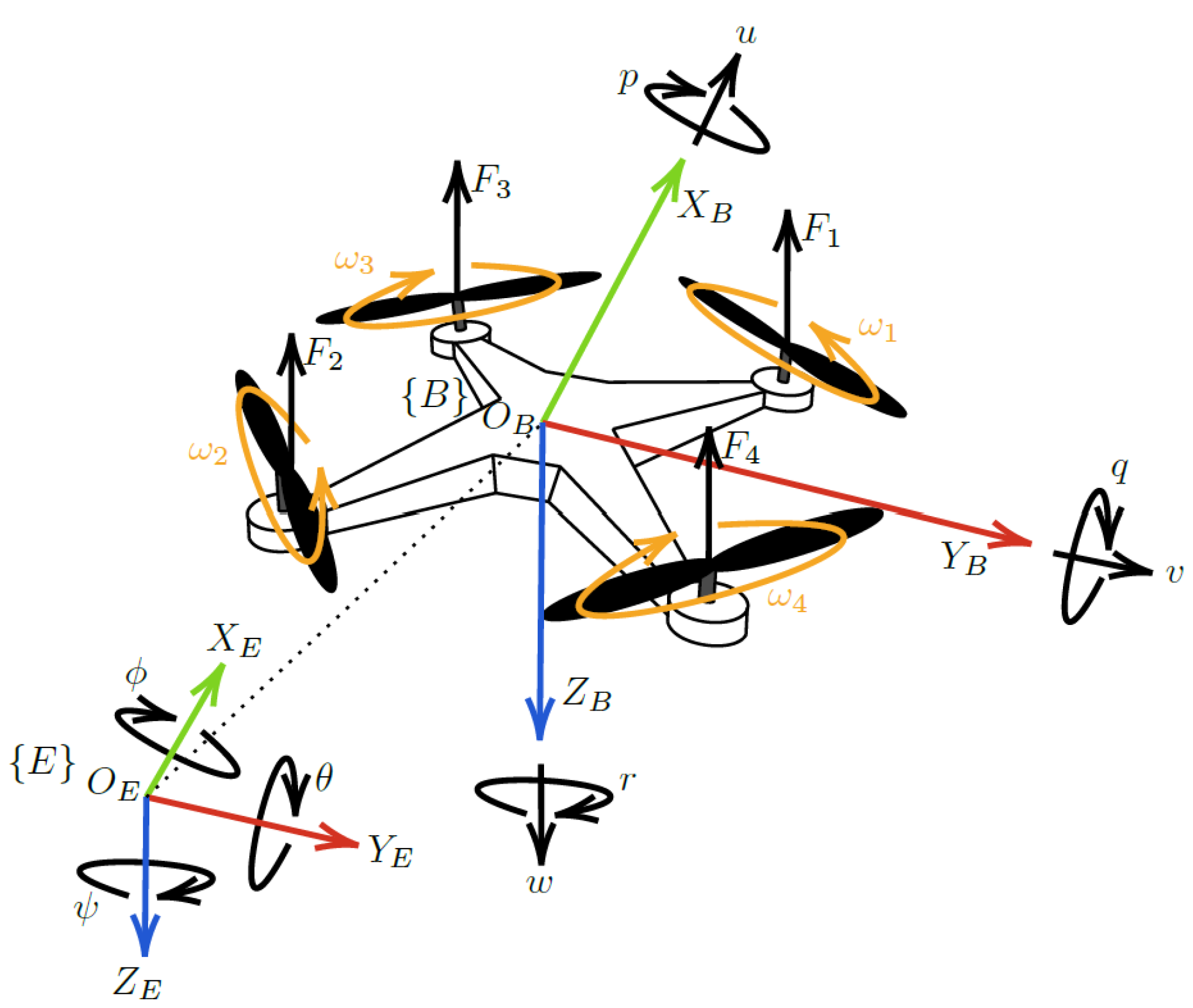
2.1. UAV Dynamic Model

A quadrotor is a four-rotor aerial vehicle that employs two coordinate systems for describing its motion: the Earth fixed frame {E}$(O_E,X_E,Y_E,Z_E)$ which is affixed to the Earth’s surface and is employed to depict motion concerning the Earth’s surface, and the Body fixed frame {B}$(O_B,X_B,Y_B,Z_B)$, which is attached to the center of mass of the quadcopter’s body and describes its motion relative to itself. As can be seen in Figure 1, four identical brushless DC motors are securely mounted on the robust, cross-shaped frame of the quadcopter. Motors 1 and 2 rotate counterclockwise, while motors 3 and 4 rotate clockwise with respect to the positive $Z_B$-axis direction at an angular velocity ${\omega }_i\ge 0$ that generates forces $F_i\ge 0(i=1,2,3,4)$ [46].

The variables states used to describe the position, velocity and attitude of the quadrotor are: $\left[pv\eta \omega \right]$, where $p={[x,y,z]}^T$ denotes the translational position vector, and $\eta ={[\varphi ,\theta ,\psi ]}^T$ denotes the UAV’s attitude with respect to {E}, where $\varphi \in [-\pi /2,\pi /2]$ is the roll angle about the $X_E$–axis, $\theta \in [-\pi /2,\pi /2]$ is the pitch angle about the $Y_E$–axis, and $\psi \in [-\pi ,\pi ]$ is the yaw angle about the $Z_E$–axis. Moreover $v={[u,v,w]}^T$ and $\omega ={[p,q,r]}^T$ are the linear and angular velocities, represented in {E} and {B}, respectively [8,47,48,49].

To transform vectors expressed in {B} into vectors expressed in {E}, the rotation matrix $R\left(\eta \right)$ and the transformation matrix $W\left(\eta \right)$ are used, respectively

$$R\left(\eta \right)=\left[\begin{array}{ccc}cos\psi cos\theta & cos\psi sin\theta sin\varphi -sin\psi cos\varphi & cos\psi sin\theta cos\varphi +sin\psi sin\varphi \\ sin\psi cos\theta & sin\psi sin\theta sin\varphi +cos\psi cos\varphi & sin\psi sin\theta cos\varphi -cos\psi sin\varphi \\ -sin\theta & cos\theta sin\varphi & cos\theta cos\varphi \end{array}\right]$$

$$W\left(\eta \right)=\left[\begin{array}{ccc}1& tan\theta sin\varphi & tan\theta cos\varphi \\ 0& cos\varphi & -sin\varphi \\ 0& sec\theta sin\varphi & sec\theta cos\varphi \end{array}\right]$$

The dynamic model is developed using the Newton-Euler method. The translational dynamics are expressed in {E}, while the rotation dynamics are expressed in {B}. Thus, the dynamic equations of motion can be represented as follows [25,50,51]

$$\begin{array}{cc}\hfill \dot{p}& =v\hfill \\ \hfill \dot{v}& ={\displaystyle \frac{1}{m}}R\left(\eta \right)F_{prop}+{\displaystyle \frac{1}{m}}{F}_{grav}+{\displaystyle \frac{1}{m}}{F}_{aero}\hfill \\ \hfill \dot{\eta }& =W\left(\eta \right)\omega \hfill \\ \hfill \dot{\omega }& =I^{-1}\left(-S_{\omega }I\omega +T_{prop}+T_{gyro}+T_{aero}\right)\hfill \end{array}$$

(1)

with m and $I=diag(Ixx,Iyy,Izz)$ which represent the mass and the inertia matrix of the UAV. $S_{\omega }\left(\omega \right)$ is the so-called dyadic representation of $\omega$, which can be expressed as a skew-symmetric matrix so-called dyadic representation of $\omega$. $F_{prop}$ and $T_{prop}$ are the forces and moments generated by the propellers. $F_{grav}$ represents the force due to the gravity, $F_{aero}$ and $T_{aero}$ denote aerodynamic forces and torques acting on the UAV due to the external disturbances, and $T_{gyro}$ defines the gyroscopic effects caused by propeller rotations. These variables are defined as

$$\begin{array}{l}{F}_{prop}=\left[\begin{array}{c}0\\ 0\\ U_1\end{array}\right]=\left[\begin{array}{c}0\\ 0\\ \sum _{i=1}^4{F}_i\end{array}\right],T_{prop}=\left[\begin{array}{c}{U}_2\\ U_3\\ U_4\end{array}\right]=\left[\begin{array}{c}{\displaystyle \frac{\sqrt{2}}{2}}l(F_1-F_2-F_3+F_4)\\ {\displaystyle \frac{\sqrt{2}}{2}}l(F_1-F_2+F_3-F_4)\\ {\kappa }_{\tau }(F_1+F_2-F_3-F_4)\end{array}\right],\\ F_{grav}=\left[\begin{array}{c}0\\ 0\\ -mg\end{array}\right],F_{aero}=\left[\begin{array}{c}{F}_x\\ F_y\\ F_z\end{array}\right],T_{aero}=\left[\begin{array}{c}{T}_{\varphi }\\ T_{\theta }\\ T_{\psi }\end{array}\right],T_{gyro}={\displaystyle \sum _{i=1}^4}{(-1)}^i{I}_r{\mathrm{\Omega }}_r{S}_{\omega }{Z}_B\end{array}$$

(2)

where the force produced by each motor is determined by $F_i={\kappa }_b{\omega }_i^2(i=1,2,3,4)$, with ${\kappa }_b$ representing the thrust factor. Additionally, l denotes the distance from the center of mass of the UAV to the motor shaft, ${\kappa }_{\tau }$ stands for the drag factor, $I_r$ corresponds to the motor inertia, ${\displaystyle {\mathrm{\Omega }}_r=-{\omega }_1-{\omega }_2+{\omega }_3+{\omega }_4}$ which represents a cross configuration, and $Z_B={\left[001\right]}^T$. Moreover, $F_j(j=x,y,z)$ denotes the aerodynamic force for each applicable vehicle orientation, computed as $F_j={\displaystyle \frac{1}{2}}\rho C_j{V}_{aw}^{2}A$, where $C_j$ represents the aerodynamic coefficients, $\rho$ stands for air density, A is the projected area of UAV element normal to the incident flow and, $V_{aw}=V-V_{wind}$ indicates the aircraft’s velocity relative to the wind [52]. Furthermore, $T_k(k=\varphi ,\theta ,\psi )$ corresponds to the aerodynamic torques induces by the aerodynamic forces estimated by $T_{aero}=l_c\times F_{aero}$, where $l_c$ corresponds to the position vector from the center of mass to the point of application of the force.

When the quadrotor Euler angles ($\varphi ,\theta ,\psi$) are considered small ($\varphi ,\theta ,\psi \approx 0$), $W\left(\eta \right)$ simplifies to the identity matrix ${\mathbf{I}}_{3x3}$. This assumption is valid because the quadcopter’s movements are gradual and gentle [53]. Therefore, the body rates equations can be approximated as $[\dot{\varphi },\dot{\theta },\dot{\psi }]\approx [p,q,r]$. This approach is detailed in [47,48].

Consequently, under the small angle assumption, and considering (1) and (2), the quadrotor’s dynamics can be summarized as

$$\begin{array}{cc}\hfill m\ddot{x}& =\left(sin\psi sin\varphi +cos\psi sin\theta cos\varphi \right)U_1+F_x\hfill \\ \hfill m\ddot{y}& =\left(-cos\psi sin\varphi +sin\psi sin\theta cos\varphi \right)U_1+F_y\hfill \\ \hfill m\ddot{z}& =-mg+\left(cos\theta cos\varphi \right)U_1+F_z\hfill \\ \hfill I_{xx}\ddot{\varphi }& =\dot{\theta }\dot{\psi }(I_{yy}-I_{zz})-I_r\dot{\theta }{\mathrm{\Omega }}_r+l{U}_2+T_{\varphi }\hfill \\ \hfill I_{yy}\ddot{\theta }& =\dot{\varphi }\dot{\psi }(I_{zz}-I_{xx})+I_r\dot{\varphi }{\mathrm{\Omega }}_r+l{U}_3+T_{\theta }\hfill \\ \hfill I_{zz}\ddot{\psi }& =\dot{\varphi }\dot{\theta }(I_{xx}-I_{yy})+U_4+T_{\psi }\hfill \end{array}$$

(3)

where the control inputs $U={[U_1,U_2,U_3,U_4]}^T$ are given by ${\displaystyle U=M{\mathrm{\Omega }}_r^2}$, where ${\displaystyle M}$ is the matrix of forces and moments generated by the motors which in this UAV configuration corresponds to

$$M=\left[\begin{array}{cccc}{\kappa }_b& {\kappa }_b& {\kappa }_b& {\kappa }_b\\ {\kappa }_p& -{\kappa }_p& -{\kappa }_p& {\kappa }_p\\ {\kappa }_p& -{\kappa }_p& {\kappa }_b& -{\kappa }_p\\ {\kappa }_{\tau }& {\kappa }_{\tau }& -{\kappa }_{\tau }& -{\kappa }_{\tau }\end{array}\right]$$

with a thrust factor ${\kappa }_b=C_{\tau }\rho D^4$ and a drag factor ${\kappa }_{\tau }=C_D\rho A/2$, where $C_{\tau }$ is the propeller’s nondimensional thrust coefficient, $C_D$ is the drag coefficient, $\rho$ is the air density, D is the propeller diameter, and A is reference area of the UAV [54]. ${\kappa }_p$ is obtained by ${\kappa }_{b}sin(\sqrt{2}/2)$ since the rotors are placed at 45 degrees from axis $X_B$ and $Y_B$ as can be seen in Figure 1.

Remark 1.

The main advantage of this approach, which involves handling the control inputs separately from the angular velocities, is related to the practicality of the controller design. Specifically, by obtaining the control inputs and applying $U=M{\mathrm{\Omega }}_r^2$ to relate them to the angular velocities, the quadrotor model remains unchanged. Only the matrix M would need to be modified to obtain the corresponding angular velocities. This method ensures flexibility and ease of implementation across various UAV configurations, allowing any designed controller to be adapted for use in other multi-rotor vehicles (with 6, 8, or different numbers of rotors) by simply changing the respective equation that links the model inputs with the rotor signals [45,55].

2.2. Actuators Dynamic Model

The motors used by the quadrotor are Brushless DC (BLDC) type. While drones typically use three-phase BLDC motors for better performance and efficiency, in this case, single-phase motors are assumed to simplify the design and reduce system complexity. This simplification allows for more straightforward modeling and control implementation, which is particularly beneficial in the initial stages of system development. The single-phase BLDC motor model reduces the number of variables and equations, making it easier to analyze and understand the fundamental dynamics of the UAV system [25,56]. These motors consist of a series circuit comprising a voltage source, resistor, inductor, and voltage drop across the motor as shown in Figure 2.

The mathematical model of a single-phase Brushless DC motor is based on electrical and mechanical equations that describe its behavior. The electrical equation used is based on Kirchhoff’s voltage law, which relates the applied voltage V, internal resistance ${\displaystyle R}$, inductance L, and the electromotive force $E_m$ generated by the motor, which depends on the angular velocity ${\omega }_m$ and is related to the electromotive constant of the motor $K_b$. On the other hand, the mechanical equation relates the external load ${\tau }_l$, the angular velocity of the motor ${\omega }_m$, and the produced torque $T_m$ which can be obtained from the motor torque constant $K_m$ multiplied by the current i. Therefore the mathematical model of the motor is summarized by

$$\begin{array}{cc}\hfill V& =Ri+L{\displaystyle \frac{\mathrm{d}}{\mathrm{dt}}}i+K_b{\omega }_m\hfill \\ \hfill J_m{\displaystyle \frac{\mathrm{d}}{\mathrm{dt}}}{\omega }_m& =K_{m}i-B_m{\omega }_m-{\tau }_l\hfill \end{array}$$

(4)

where $J_m$ refers to motor moment of inertia and $B_m$ is the damping coefficient.

3. Design of a Nonlinear Control with Perfectly Known Parameters

The control strategy considers two control loops, an inner loop is used for the UAV’s actuators and an outer loop for the UAV frame. The overall control goal is to follow the reference vector $p_{ref}$ using the vehicle’s output p. To do this, a UAV controller (outer control loop) that generates the required angular velocities for the actuators ${\omega }_{m,ref}$ is created. After then, the actuators controller (inner control loop) is made to track the references ${\omega }_{m,ref}$ using the actual angular velocities of the actuators ${\omega }_m$. In this case, both are PI–like controllers to simplify their operation.

3.1. UAV Controller

Applying a PI-like controller for the trajectory of a UAV involves designing a control system that allows the drone to follow a desired route in a precise and stable manner. In our control approach, we have divided the task into two fundamental stages: position and attitude control.

The position controller is defined considering the error variable $e_p=p-p_{ref}$, where the control problem consists of designing a controller such that $\underset{t\to \infty }{lim}{e}_p=0$. This controller is broken down into three main components. We will call the first subsystem $S_1$, which is responsible for controlling the altitude of the UAV. The second component, known as subsystem $S_2$, is used for controlling the displacement on the $X_E$-axis by imposing ${\theta }_{ref}$ to the attitude controller. Finally the third, subsystem $S_3$, controls linear displacement in the $Y_E$-axis by imposing ${\varphi }_{ref}$ to the attitude controller.

On the other hand, the attitude controller is responsible for controlling the roll ($\varphi$), pitch ($\theta$), and yaw ($\psi$) movements by considering the error variable $e_{\eta }=\eta -{\eta }_{ref}$ where the controller aim is that $\underset{t\to \infty }{lim}{e}_{\eta }=0$. From this controller we can consider a fourth subsystem called $S_4$, used to exclusively control the yaw movement.

Taking the aforementioned into account and introducing some variable modifications in (3), where $x=x_1$, ${\dot{x}}_1=x_2$, $y=y_1$, ${\dot{y}}_1=y_2$, $z=z_1$, ${\dot{z}}_1=z_2$, $\varphi ={\varphi }_1$, ${\dot{\varphi }}_1={\varphi }_2$, $\theta ={\theta }_1$, ${\dot{\theta }}_1={\theta }_2$, $\psi ={\psi }_1$, ${\dot{\psi }}_1={\psi }_2$, we obtain

$$\begin{array}{cc}{S}_1\hfill & =\left\{\begin{array}{c}{\dot{z}}_1=z_2\hfill \\ {\dot{z}}_2=-g+\left(cos{\theta }_{1}cos{\varphi }_1\right){\displaystyle \frac{U_1}{m}}+{\displaystyle \frac{F_z}{m}}\hfill \end{array}\right.\hfill \\ S_2\hfill & =\left\{\begin{array}{c}{\dot{x}}_1=x_2\hfill \\ {\dot{x}}_2=\left(sin{\psi }_{1}sin{\varphi }_1+cos{\psi }_{1}sin{\theta }_{1}cos{\varphi }_1\right){\displaystyle \frac{U_1}{m}}+{\displaystyle \frac{F_x}{m}}\hfill \\ {\dot{\theta }}_1={\theta }_2\hfill \\ {\dot{\theta }}_2=\left({\varphi }_2{\psi }_2(I_{zz}-I_{xx})+I_r{\varphi }_2{\mathrm{\Omega }}_r+l{U}_3+T_{\theta }\right)/I_{yy}\hfill \end{array}\right.\hfill \\ S_3\hfill & =\left\{\begin{array}{c}{\dot{y}}_1=y_2\hfill \\ {\dot{y}}_2=\left(-cos{\psi }_{1}sin{\varphi }_1+sin{\psi }_{1}sin{\theta }_{1}cos{\varphi }_1\right){\displaystyle \frac{U_1}{m}}+{\displaystyle \frac{F_y}{m}}\hfill \\ {\dot{\varphi }}_1={\varphi }_2\hfill \\ {\dot{\varphi }}_2=\left({\theta }_2{\psi }_2(I_{yy}-I_{zz})-I_r{\theta }_2{\mathrm{\Omega }}_r+l{U}_2+T_{\varphi }\right)/I_{xx}\hfill \end{array}\right.\hfill \\ S_4\hfill & =\left\{\begin{array}{c}{\dot{\psi }}_1={\psi }_2\hfill \\ {\dot{\psi }}_2=\left({\varphi }_2{\theta }_2(I_{xx}-I_{yy})+U_4+T_{\psi }\right)/I_{zz}\hfill \end{array}\right.\hfill \end{array}$$

(5)

Assumption 1.

We assume that all variables for the control of the UAV are measured accurately.

This assumption is justified based on the availability and reliability of modern sensor technologies used in UAVs. GPS systems provide accurate global positioning data for outdoor environments, while motion capture and ultra-wideband (UWB) localization systems offer high-precision position measurements for indoor applications. Attitude data, including roll, pitch, and yaw angles, are obtained from Inertial Measurement Units (IMUs) that combine accelerometers and gyroscopes, with magnetometer readings often integrated through sensor fusion algorithms like the Kalman filter to enhance accuracy. Linear velocity can be derived by differentiating position data or integrating acceleration data from IMUs, and angular velocity is directly measured by gyroscopes within the IMU. The aerodynamic forces ($F_x,F_y,F_z$) and moments ($T_{\varphi },T_{\theta },T_{\psi }$) are known from measurements obtained using pitot tubes. Pitot tubes measure the airspeed relative to the UAV, which allows the calculation of different aerodynamic forces and, subsequently, the corresponding torques due to the wind. These advanced measurement technologies ensure that the UAV’s state variables are reliably known, thereby supporting effective and stable flight control.

By using the error variable $e_p=p-p_{ref}$ of the position controller and considering (5), we can obtain the tracking error for subsystems $S_1$, $S_2$, and $S_3$ as $e_{z_1}=z_1-z_{1,ref}$, $e_{x_1}=x_1-x_{1,ref}$ and $e_{y_1}=y_1-y_{1,ref}$ respectively. The dynamics of these errors are given by

$${\dot{e}}_{z_1}=z_2-{\dot{z}}_{1,ref}$$

(6)

$${\dot{e}}_{x_1}=x_2-{\dot{x}}_{1,ref}$$

(7)

$${\dot{e}}_{y_1}=y_2-{\dot{y}}_{1,ref}$$

(8)

The given control problem will be solved under the following assumption.

Assumption 2.

The reference signals $z_{1,ref}$, $x_{1,ref}$ and $y_{1,ref}$ and their derivatives ${\dot{z}}_{1,ref}$, ${\dot{x}}_{1,ref}$ and ${\dot{y}}_{1,ref}$ are bounded.

In the Assumption 2, the signals $z_{1,ref}$, $x_{1,ref}$ and $y_{1,ref}$ are assumed to be constant and are considered bounded since they have fixed values that do not change over time. Consequently, their derivatives ${\dot{z}}_{1,ref}$, ${\dot{x}}_{1,ref}$ and ${\dot{y}}_{1,ref}$ are also considered bounded.

Without loss of generality and following the same order of subsystems in (5), the virtual controls $-k_{z_1}{e}_{z_1}-k_{0,z_1}I{e}_{z_1}=z_{2,d}-{\dot{z}}_{1,ref}$; $-k_{x_1}{e}_{x_1}-k_{0,x_1}I{e}_{x_1}=x_{2,d}-{\dot{x}}_{1,ref}$ and $-k_{y_1}{e}_{y_1}-k_{0,y_1}I{e}_{y_1}=y_{2,d}-{\dot{y}}_{1,ref}$ are used, where $I{e}_j$ is an integrative term defined by ${\dot{Ie}}_j=e_j$, $k_{j_1}$ corresponds to the proportional gain and $k_{0,j_1}$ is the integral gain with $j=z,x,y$. In this manner it is feasible to get $z_{2,d}$, $x_{2,d}$ and $y_{2,d}$ as follows

$$z_{2,d}={\dot{z}}_{1,ref}-k_{z_1}{e}_{z_1}-k_{0,z_1}I{e}_{z_1}$$

(9)

$$x_{2,d}={\dot{x}}_{1,ref}-k_{x_1}{e}_{x_1}-k_{0,x_1}I{e}_{x_1}$$

(10)

$$y_{2,d}={\dot{y}}_{1,ref}-k_{y_1}{e}_{y_1}-k_{0,y_1}I{e}_{y_1}$$

(11)

Now we can define the errors $e_{z_2}=z_2-z_{2,d}$, $e_{x_2}=x_2-x_{2,d}$ and $e_{y_2}=y_2-y_{2,d}$ and upon derivation, we obtain ${\dot{e}}_{z_2}={\dot{z}}_2-{\dot{z}}_{2,d}$, ${\dot{e}}_{x_2}={\dot{x}}_2-{\dot{x}}_{2,d}$ and ${\dot{e}}_{y_2}={\dot{y}}_2-{\dot{y}}_{2,d}$. Therefore, the dynamics of the tracking error of $S_1$, $S_2$, and $S_3$ can be expressed as

$${\dot{e}}_{z_2}=-g+{\displaystyle \frac{1}{m}}cos{\theta }_{1}cos{\varphi }_1{U}_1+{\displaystyle \frac{F_z}{m}}-{\dot{z}}_{2,d}$$

(12)

$${\dot{e}}_{x_2}={\displaystyle \frac{1}{m}}(sin{\psi }_{1}sin{\varphi }_1+cos{\psi }_{1}sin{\theta }_{1}cos{\varphi }_1)U_1+{\displaystyle \frac{F_x}{m}}-{\dot{x}}_{2,d}$$

(13)

$${\dot{e}}_{y_2}={\displaystyle \frac{1}{m}}(-cos{\psi }_{1}sin{\varphi }_1+sin{\psi }_{1}sin{\theta }_{1}cos{\varphi }_1)U_1+{\displaystyle \frac{F_y}{m}}-{\dot{y}}_{2,d}$$

(14)

where ${\dot{z}}_{2,d}={\ddot{z}}_{1,ref}-k_{z_1}{\dot{e}}_{z_1}-k_{0,z_1}\dot{I}{e}_{z_1}$, ${\dot{x}}_{2,d}={\ddot{x}}_{1,ref}-k_{x_1}{\dot{e}}_{x_1}-k_{0,x_1}\dot{I}{e}_{x_1}$ and ${\dot{y}}_{2,d}={\ddot{y}}_{1,ref}-k_{y_1}{\dot{e}}_{y_1}-k_{0,y_1}\dot{I}{e}_{y_1}$.

However, in order to achieve $\underset{t\to \infty }{lim}{e}_x=0$ and $\underset{t\to \infty }{lim}{e}_y=0$, which ensures accurate tracking of translation along the x and y axes, it is essential to control the inclination angles pitch (${\theta }_1$) and roll (${\varphi }_1$) respectively. In this manner, by the stabilization of $e_{z_1}$, $e_{x_1}$ and $e_{y_1}$, the reference values for $sin{\theta }_1$ and $sin{\varphi }_1$ can be fixed as follows

$$\begin{array}{cc}\hfill sin{\theta }_{1,d}& ={\displaystyle \frac{m}{cos{\varphi }_{1}cos{\psi }_1{U}_1}}({\dot{x}}_{2,d}-{\displaystyle \frac{1}{m}}(sin{\varphi }_{1}sin{\psi }_1)U_1-{\displaystyle \frac{F_x}{m}}\hfill \\ \hfill & -k_{x_2}{e}_{x_2}-k_{0,x_2}I{e}_{x_2})\hfill \end{array}$$

(15)

$$\begin{array}{cc}\hfill sin{\varphi }_{1,d}& =-{\displaystyle \frac{m}{cos{\psi }_1{U}_1}}({\dot{y}}_{2,d}-{\displaystyle \frac{1}{m}}(cos{\varphi }_{1}sin{\theta }_{1}sin{\psi }_1)U_1-{\displaystyle \frac{F_y}{m}}\hfill \\ \hfill & -k_{y_2}{e}_{y_2}-k_{0,y_2}I{e}_{y_2})\hfill \end{array}$$

(16)

In this way, to impose the references, ${\theta }_1$ and ${\varphi }_1$ are now treated as tracking errors as depicted below

$$\begin{array}{cc}\hfill e_{{\varphi }_1}& =sin{\varphi }_1-sin{\varphi }_{1,d}\hfill \end{array}$$

(17)

$$\begin{array}{cc}\hfill e_{{\theta }_1}& =sin{\theta }_1-sin{\theta }_{1,d}\hfill \end{array}$$

(18)

Here, $sin{\varphi }_{1,d}$ and $sin{\theta }_{1,d}$ represent the desired values of the sine of the roll and pitch angles, respectively. Hence ${\varphi }_{1,d}=arcsin{\varphi }_{1,d}$ and ${\theta }_{1,d}=arcsin{\theta }_{1,d}$.

Through derivation of (17) and (18), and by applying the chain rule of differentiation, we obtain the dynamics of the errors which are given by

$${\dot{e}}_{{\varphi }_1}=cos{\varphi }_1{\varphi }_2-{\displaystyle \frac{\mathrm{d}}{\mathrm{dt}}}{sin\varphi }_{1,d}$$

(19)

$${\dot{e}}_{{\theta }_1}=cos{\theta }_1{\theta }_2-{\displaystyle \frac{\mathrm{d}}{\mathrm{dt}}}{sin\theta }_{1,d}$$

(20)

By the utilization of the virtual controls $-k_{{\varphi }_1}{e}_{{\varphi }_1}-k_{0,{\varphi }_1}I{e}_{{\varphi }_1}=cos{\varphi }_1{\varphi }_{2,d}-{\displaystyle \frac{\mathrm{d}}{\mathrm{dt}}}sin{\varphi }_{1,d}$ for (17), and $-k_{{\theta }_1}{e}_{{\theta }_1}-k_{0,{\theta }_1}I{e}_{{\theta }_1}=cos{\theta }_1{\theta }_{2,d}-{\displaystyle \frac{\mathrm{d}}{\mathrm{dt}}}{sin\theta }_{1,d}$ for (18), where $I{e}_k$ is an integrative term defined by ${\dot{Ie}}_k=e_k$, $k_{k_1}$ corresponds to the proportional gain and $k_{0,k_1}$ is the integral gain with $k={\varphi }_1,{\theta }_1$, it is feasible to get ${\varphi }_{2,d}$ and ${\theta }_{2,d}$ as follows

$${\varphi }_{2,d}={\displaystyle \frac{1}{cos{\varphi }_1}}\left({\displaystyle \frac{\mathrm{d}}{\mathrm{dt}}}sin{\varphi }_{1,d}-k_{{\varphi }_1}{e}_{{\varphi }_1}-k_{0,{\varphi }_1}I{e}_{{\varphi }_1}\right)$$

(21)

$${\theta }_{2,d}={\displaystyle \frac{1}{cos{\theta }_1}}\left({\displaystyle \frac{\mathrm{d}}{\mathrm{dt}}}sin{\theta }_{1,d}-k_{{\theta }_1}{e}_{{\theta }_1}-k_{0,{\theta }_1}I{e}_{{\theta }_1}\right)$$

(22)

Now, by defining the tracking errors $e_{{\varphi }_2}={\varphi }_2-{\varphi }_{2,d}$, $e_{{\theta }_2}={\theta }_2-{\theta }_{2,d}$ and their respective derivation ${\dot{e}}_{{\varphi }_2}={\dot{\varphi }}_2-{\dot{\varphi }}_{2,d}$, ${\dot{e}}_{{\theta }_2}={\dot{\theta }}_2-{\dot{\theta }}_{2,d}$, the error dynamics are obtained

$${\dot{e}}_{{\varphi }_2}=\left({\displaystyle \frac{I_{yy}-I_{zz}}{I_{xx}}}\right){\theta }_2{\psi }_2-{\displaystyle \frac{I_r}{I_{xx}}}{\theta }_2{\mathrm{\Omega }}_r+{\displaystyle \frac{l}{I_{xx}}}{U}_2+{\displaystyle \frac{T_{\varphi }}{I_{xx}}}-{\dot{\varphi }}_{2,d}$$

(23)

$${\dot{e}}_{{\theta }_2}=\left({\displaystyle \frac{I_{zz}-I_{xx}}{I_{yy}}}\right){\varphi }_2{\psi }_2+{\displaystyle \frac{I_r}{I_{yy}}}{\varphi }_2{\mathrm{\Omega }}_r+{\displaystyle \frac{l}{I_{yy}}}{U}_3+{\displaystyle \frac{T_{\theta }}{I_{yy}}}-{\dot{\theta }}_{2,d}$$

(24)

On the other hand, through the utilization of the error variable $e_{\eta }=\eta -{\eta }_{ref}$ of the attitude controller and considering (5), we can derive the tracking error for the subsystem $S_4$ as $e_{{\psi }_1}={\psi }_1-{\psi }_{1,ref}$. The dynamics of this error is given by ${\dot{e}}_{{\psi }_1}={\psi }_2-{\dot{\psi }}_{1,ref}$. Hence, through the utilization of the virtual control ${\displaystyle -k_{{\psi }_1}{e}_{{\psi }_1}-k_{0,{\psi }_1}I{e}_{{\psi }_1}={\psi }_{2,d}-{\dot{\psi }}_{1,ref}}$, the dynamics of the tracking error in the subsystem $S_4$ can be seen as follows

$$\begin{array}{cc}\hfill {\dot{e}}_{{\psi }_2}& =\left({\displaystyle \frac{I_{xx}-I_{yy}}{I_{zz}}}\right){\varphi }_2{\theta }_2+{\displaystyle \frac{U_4}{I_{zz}}}+{\displaystyle \frac{T_{\psi }}{I_{zz}}}-{\dot{\psi }}_{2,d}\hfill \end{array}$$

(25)

where ${\dot{\psi }}_{2,d}={\ddot{\psi }}_{1,ref}-k_{{\psi }_1}{\dot{e}}_{{\psi }_1}-k_{0,{\psi }_1}{\dot{Ie}}_{{\psi }_1}$.

Therefore, based on (12), (23), (24), and (25), the proposed control inputs are

$$\begin{array}{cc}\hfill U_1& ={\displaystyle \frac{m}{cos{\theta }_{1}cos{\varphi }_1}}\left({\dot{z}}_{2,d}+g-{\displaystyle \frac{F_z}{m}}-k_{z_2}{e}_{z_2}-k_{0,z_2}{Ie}_{z_2}\right)\hfill \\ \hfill U_2& ={\displaystyle \frac{I_{xx}}{l}}\left({\dot{\varphi }}_{2,d}-{\displaystyle \frac{{\theta }_2{\psi }_2(I_{yy}-I_{zz})}{I_{xx}}}+{\displaystyle \frac{I_r{\theta }_2{\mathrm{\Omega }}_r}{I_{xx}}}-{\displaystyle \frac{T_{\varphi }}{I_{xx}}}-k_{{\varphi }_2}{e}_{{\varphi }_2}-k_{0,{\varphi }_2}{Ie}_{{\varphi }_2}\right)\hfill \\ \hfill U_3& ={\displaystyle \frac{I_{yy}}{l}}\left({\dot{\theta }}_{2,d}-{\displaystyle \frac{{\varphi }_2{\psi }_2(I_{zz}-I_{xx})}{I_{yy}}}-{\displaystyle \frac{I_r{\varphi }_2{\mathrm{\Omega }}_r}{I_{yy}}}-{\displaystyle \frac{T_{\theta }}{I_{yy}}}-k_{{\theta }_2}{e}_{{\theta }_2}-k_{0,{\theta }_2}{Ie}_{{\theta }_2}\right)\hfill \\ \hfill U_4& =I_{zz}\left({\dot{\psi }}_{2,d}-{\displaystyle \frac{{\varphi }_2{\theta }_2(I_{xx}-I_{yy})}{I_{zz}}}-{\displaystyle \frac{T_{\psi }}{I_{zz}}}-k_{{\psi }_2}{e}_{{\psi }_2}-k_{0,{\psi }_2}{Ie}_{{\psi }_2}\right)\hfill \end{array}$$

(26)

where $k_i,k_{0,i}>0$, $i=z_2,{\varphi }_2,{\theta }_2,{\psi }_2$.

To establish a strong connection between the UAV controller and the actuators, it is essential to convert the control signals produced by (26) into reference angular velocities that the actuators can interpret and execute. This transformation is accomplished through the resolution of ${\mathrm{\Omega }}_r$ from ${\displaystyle U=M{\mathrm{\Omega }}_r^2}$.

3.2. Actuators Controller

As mentioned in Section 2.1, the quadcopter is equipped with four identical motors, operating according to the dynamics defined by Equation (4).

Assumption 3.

We assume that all variables for the control of the BLDC motor are measured accurately.

This assumption is justified based on the advanced measurement technologies and control systems available for BLDC motors. The rotor speed (${\omega }_{m,i}$) and load torque (${\tau }_{l,i}$) are typically measured using rotary encoders and torque sensors, respectively. The current ($i_i$) is measured using current sensors such as Hall effect sensors. The inertia ($J_{m,i}$), damping coefficient ($B_{m,i}$), motor constant ($K_{m,i}$), back-EMF constant ($K_{b,i}$), resistance ($R_i$), and inductance ($L_i$) are known from the motor specifications provided by the manufacturer. The voltage ($V_i$) is measured using voltage sensors. These technologies and methods ensure that all relevant variables are accurately known, supporting precise and effective control of the BLDC motor.

In this framework, a PI–like controller for the actuators is formulated to guarantee that the angular velocities of the motors, ${\displaystyle {\omega }_{m,i},i=1,\dots ,4}$, closely track the desired references. Therefore, $\underset{t\to \infty }{lim}{e}_{\omega ,m,i}=0$, considering the error variable ${\displaystyle e_{\omega ,m,i}={\omega }_{m,i}-{\omega }_{m,i,ref}}$.

Therefore, from (4) it is possible to obtain the error dynamics as follows

$$\begin{array}{c}\hfill {\dot{e}}_{\omega ,m,i}={\displaystyle \frac{K_{m,i}}{J_{m,i}}}{i}_i-{\displaystyle \frac{B_{m,i}}{J_{m,i}}}{\omega }_{m,i}-{\displaystyle \frac{{\tau }_{l,i}}{J_{m,i}}}-{\displaystyle \frac{\mathrm{d}}{\mathrm{dt}}}{\omega }_{m,i,ref}\end{array}$$

(27)

where it is necessary to impose the current by

$$\begin{array}{c}\hfill i_{i,ref}={\displaystyle \frac{J_{m,i}}{K_{m,i}}}({\displaystyle \frac{B_{m,i}{\omega }_{m,i}}{J_{m,i}}}+{\displaystyle \frac{{\tau }_{l,i}}{J_{m,i}}}+{\dot{\omega }}_{i,ref}-k_{\omega ,i}{e}_{\omega ,i}-k_{0,\omega ,i}{Ie}_{\omega ,i})\end{array}$$

(28)

with $k_{\omega ,i},k_{0,\omega ,i}>0$, where the PI–like controller have been applied. Finally, it is possible to get the current error dynamics by considering the current error ${\displaystyle e_{i,i}=i_i-i_{i,ref}}$, such that $\underset{t\to \infty }{lim}{e}_{i,i}=0$

$$\begin{array}{c}\hfill {\dot{e}}_{i,i}={\displaystyle \frac{1}{L_i}}(-R_i{i}_i-{\displaystyle \frac{K_{b,i}{\omega }_{m,i}}{L_i}}+V_i)-{\displaystyle \frac{\mathrm{d}}{\mathrm{dt}}}{i}_{i,ref}\end{array}$$

(29)

from where it is possible to derive the voltage input which has to be applied to the motor

$$\begin{array}{cc}\hfill V_i& =L_i({\displaystyle \frac{R_i{i}_i}{L_i}}+{\displaystyle \frac{K_{b,i}{\omega }_{m,i}}{L_i}}+{\displaystyle \frac{\mathrm{d}}{\mathrm{dt}}}{i}_{i,ref}-k_{i,i}{e}_{i,i}-k_{0,i,i}{Ie}_{i,i})\hfill \end{array}$$

(30)

with $k_{i,i},k_{0,i,i}>0$.

4. Design of a Robust Nonlinear Control with Estimation of Disturbances and Parameter Uncertainties

In this section, a robust control is designed to address uncertainties in system parameters and the presence of external disturbances. The proposed control strategy aims to enhance the stability and performance of the UAV despite variations in system dynamics and external factors that could potentially disrupt its operation.

The robust control framework integrates nonlinear control techniques and disturbance estimation strategies to dynamically adapt to changing environmental conditions. By incorporating PI-like controllers within both the outer and inner control loops, the system effectively mitigates the impact of uncertainties and disturbances on the UAV’s performance.

A general schematic of the proposed robust control system is shown in Figure 3. This diagram illustrates the interaction between the various components of the control architecture, including the measurement of state variables, the generation of control inputs, and the implementation of feedback mechanisms to ensure precise trajectory tracking and stable flight performance.

4.1. UAV Robust Control with Disturbance Estimation

To achieve robustness of the closed–loop system with respect to parameter variations and external disturbances, the dynamics of the tracking errors of the system (12)–(14), and (23)–(25) are rewritten

$$\begin{array}{cc}\hfill {\dot{e}}_{z_2}& =-g+{\displaystyle \frac{1}{m^{\circ }}}(cos{\theta }_{1}cos{\varphi }_1)U_1+{\displaystyle \frac{{F_z}^{\circ }}{m^{\circ }}}-{\dot{z}}_{2,d}+{\delta }_{z_1}\hfill \\ \hfill {\dot{e}}_{x_2}& ={\displaystyle \frac{1}{m^{\circ }}}(sin{\psi }_{1}sin{\varphi }_1+cos{\psi }_{1}sin{\theta }_{1}cos{\varphi }_1)U_1+{\displaystyle \frac{{F_x}^{\circ }}{m^{\circ }}}-{\dot{x}}_{2,d}+{\delta }_{x_1}\hfill \\ \hfill {\dot{e}}_{y_2}& ={\displaystyle \frac{1}{m^{\circ }}}(sin{\psi }_{1}sin{\theta }_{1}cos{\varphi }_1-cos{\psi }_{1}sin{\varphi }_1)U_1+{\displaystyle \frac{{F_y}^{\circ }}{m^{\circ }}}-{\dot{y}}_{2,d}+{\delta }_{y_1}\hfill \\ \hfill {\dot{e}}_{{\varphi }_2}& =\left({\displaystyle \frac{{I_{yy}}^{\circ }-{I_{zz}}^{\circ }}{{I_{xx}}^{\circ }}}\right){\theta }_2{\psi }_2-{\displaystyle \frac{{I_r}^{\circ }}{{I_{xx}}^{\circ }}}{\theta }_2{\mathrm{\Omega }}_r+{\displaystyle \frac{l}{{I_{xx}}^{\circ }}}{U}_2+{\displaystyle \frac{{T_{\varphi }}^{\circ }}{{I_{xx}}^{\circ }}}-{\dot{\varphi }}_{2,d}+{\delta }_{{\varphi }_1}\hfill \\ \hfill {\dot{e}}_{{\theta }_2}& =\left({\displaystyle \frac{{I_{zz}}^{\circ }-{I_{xx}}^{\circ }}{{I_{yy}}^{\circ }}}\right){\varphi }_2{\psi }_2+{\displaystyle \frac{{I_r}^{\circ }}{{I_{yy}}^{\circ }}}{\varphi }_2{\mathrm{\Omega }}_r+{\displaystyle \frac{l}{{I_{yy}}^{\circ }}}{U}_3+{\displaystyle \frac{{T_{\theta }}^{\circ }}{{I_{yy}}^{\circ }}}-{\dot{\theta }}_{2,d}+{\delta }_{{\theta }_1}\hfill \\ \hfill {\dot{e}}_{{\psi }_2}& =\left({\displaystyle \frac{{I_{xx}}^{\circ }-{I_{yy}}^{\circ }}{{I_{zz}}^{\circ }}}\right){\varphi }_2{\theta }_2+{\displaystyle \frac{U_4}{{I_{zz}}^{\circ }}}+{\displaystyle \frac{{T_{\psi }}^{\circ }}{{I_{zz}}^{\circ }}}-{\dot{\psi }}_{2,d}+{\delta }_{{\psi }_1}\hfill \end{array}$$

(31)

with

$$\begin{array}{cc}\hfill {\delta }_{z_1}& =\left({\displaystyle \frac{1}{m}}-{\displaystyle \frac{1}{m^{\circ }}}\right)\left(cos{\theta }_{1}cos{\varphi }_1\right)U_1+\left({\displaystyle \frac{F_z}{m}}-{\displaystyle \frac{{F_z}^{\circ }}{m^{\circ }}}\right)\hfill \\ \hfill {\delta }_{x_1}& =\left({\displaystyle \frac{1}{m}}-{\displaystyle \frac{1}{m^{\circ }}}\right)\left(sin{\psi }_{1}sin{\varphi }_1+cos{\psi }_{1}sin{\theta }_{1}cos{\varphi }_1\right)U_1+\left({\displaystyle \frac{F_x}{m}}-{\displaystyle \frac{{F_x}^{\circ }}{m^{\circ }}}\right)\hfill \\ \hfill {\delta }_{y_1}& =\left({\displaystyle \frac{1}{m}}-{\displaystyle \frac{1}{m^{\circ }}}\right)\left(sin{\psi }_{1}sin{\theta }_{1}cos{\varphi }_1-cos{\psi }_{1}sin{\varphi }_1\right)U_1+\left({\displaystyle \frac{F_y}{m}}-{\displaystyle \frac{{F_y}^{\circ }}{m^{\circ }}}\right)\hfill \\ \hfill {\delta }_{{\varphi }_1}& =\left({\displaystyle \frac{I_{yy}-I_{zz}}{I_{xx}}}-{\displaystyle \frac{{I_{yy}}^{\circ }-{I_{zz}}^{\circ }}{{I_{xx}}^{\circ }}}\right){\theta }_2{\psi }_2-\left({\displaystyle \frac{I_r}{I_{xx}}}-{\displaystyle \frac{{I_r}^{\circ }}{{I_{xx}}^{\circ }}}\right){\theta }_2{\mathrm{\Omega }}_r\hfill \\ & +\left({\displaystyle \frac{l}{I_{xx}}}-{\displaystyle \frac{l}{{I_{xx}}^{\circ }}}\right)U_2+\left({\displaystyle \frac{T_{\varphi }}{I_{xx}}}-{\displaystyle \frac{{T_{\varphi }}^{\circ }}{{I_{xx}}^{\circ }}}\right)\hfill \\ \hfill {\delta }_{{\theta }_1}& =\left({\displaystyle \frac{I_{zz}-I_{xx}}{I_{yy}}}-{\displaystyle \frac{{I_{zz}}^{\circ }-{I_{xx}}^{\circ }}{{I_{yy}}^{\circ }}}\right){\varphi }_2{\psi }_2+\left({\displaystyle \frac{I_r}{I_{yy}}}-{\displaystyle \frac{{I_r}^{\circ }}{{I_{yy}}^{\circ }}}\right){\varphi }_2{\mathrm{\Omega }}_r\hfill \\ & +\left({\displaystyle \frac{l}{I_{xx}}}-{\displaystyle \frac{l}{{I_{yy}}^{\circ }}}\right)U_3+\left({\displaystyle \frac{T_{\theta }}{I_{yy}}}-{\displaystyle \frac{{T_{\theta }}^{\circ }}{{I_{yy}}^{\circ }}}\right)\hfill \\ \hfill {\delta }_{{\psi }_1}& =\left({\displaystyle \frac{I_{xx}-I_{yy}}{I_{zz}}}-{\displaystyle \frac{{I_{xx}}^{\circ }-{I_{yy}}^{\circ }}{{I_{zz}}^{\circ }}}\right){\varphi }_2{\theta }_2+\left({\displaystyle \frac{1}{I_{zz}}}-{\displaystyle \frac{1}{{I_{zz}}^{\circ }}}\right)U_4+\left({\displaystyle \frac{T_{\psi }}{I_{zz}}}-{\displaystyle \frac{{T_{\psi }}^{\circ }}{{I_{zz}}^{\circ }}}\right)\hfill \end{array}$$

(32)

Remark 2.

Within the vectors ${\delta }_j$ and ${\delta }_k$ there are the parametric variations and the external disturbances.

The following statement solves the posed control problem with estimation the variation of external disturbances, where ${\lfloor ·\rceil }^{1/2}={|·|}^{1/2}\mathrm{sign}(·)$, ${\lfloor ·\rceil }^0=\mathrm{sign}(·)$

Theorem 1.

Under Assumptions 1 and 2, the robust control

$$\begin{array}{cc}\hfill {\dot{\xi }}_{z_1}& =-{\lambda }_{z_1}{\lfloor {\xi }_{z_1}-e_{z_1}\rceil }^{1/2}+{\xi }_{z_2}+{\displaystyle \frac{1}{m^{\circ }}}\left(cos{\theta }_{1}cos{\varphi }_1\right)U_1+{\displaystyle \frac{{F_z}^{\circ }}{m^{\circ }}}-g-{\dot{z}}_{2,d}\hfill \\ \hfill {\dot{\xi }}_{z_2}& =-{\lambda }_{z_2}{\lfloor {\xi }_{z_1}-e_{z_1}\rceil }^0\hfill \\ \hfill {\dot{\xi }}_{x_1}& =-{\lambda }_{x_1}{\lfloor {\xi }_{x_1}-e_{x_1}\rceil }^{1/2}+{\xi }_{x_2}+{\displaystyle \frac{1}{m^{\circ }}}\left(sin{\psi }_{1}sin{\varphi }_1+cos{\psi }_{1}sin{\theta }_{1}cos{\varphi }_1\right)U_1\hfill \\ & +{\displaystyle \frac{{F_x}^{\circ }}{m^{\circ }}}-{\dot{x}}_{2,d}\hfill \\ \hfill {\dot{\xi }}_{x_2}& =-{\lambda }_{x_2}{\lfloor {\xi }_{x_1}-e_{x_1}\rceil }^0\hfill \\ \hfill {\dot{\xi }}_{y_1}& =-{\lambda }_{y_1}{\lfloor {\xi }_{y_1}-e_{y_1}\rceil }^{1/2}+{\xi }_{y_2}+{\displaystyle \frac{1}{m^{\circ }}}\left(sin{\psi }_{1}sin{\theta }_{1}cos{\varphi }_1-cos{\psi }_{1}sin{\varphi }_1\right)U_1\hfill \\ & +{\displaystyle \frac{{F_y}^{\circ }}{m^{\circ }}}-{\dot{y}}_{2,d}\hfill \\ \hfill {\dot{\xi }}_{y_2}& =-{\lambda }_{y_2}{\lfloor {\xi }_{y_1}-e_{y_1}\rceil }^0\hfill \\ \hfill {\dot{\xi }}_{{\varphi }_1}& =-{\lambda }_{{\varphi }_1}{\lfloor {\xi }_{{\varphi }_1}-e_{{\varphi }_1}\rceil }^{1/2}+{\xi }_{{\varphi }_2}+\left({\displaystyle \frac{{I_{yy}}^{\circ }-{I_{zz}}^{\circ }}{{I_{xx}}^{\circ }}}\right){\theta }_2{\psi }_2-\left({\displaystyle \frac{{I_r}^{\circ }}{{I_{xx}}^{\circ }}}\right){\theta }_2{\mathrm{\Omega }}_r\hfill \\ & +{\displaystyle \frac{l^{\circ }}{{I_{xx}}^{\circ }}}{U}_2+{\displaystyle \frac{{T_{\varphi }}^{\circ }}{{I_{xx}}^{\circ }}}-{\dot{\varphi }}_{2,d}\hfill \\ \hfill {\dot{\xi }}_{{\varphi }_2}& =-{\lambda }_{{\varphi }_2}{\lfloor {\xi }_{{\varphi }_1}-e_{{\varphi }_1}\rceil }^0\hfill \\ \hfill {\dot{\xi }}_{{\theta }_1}& =-{\lambda }_{{\theta }_1}{\lfloor {\xi }_{{\theta }_1}-e_{{\theta }_1}\rceil }^{1/2}+{\xi }_{{\theta }_2}+\left({\displaystyle \frac{{I_{zz}}^{\circ }-{I_{xx}}^{\circ }}{{I_{yy}}^{\circ }}}\right){\varphi }_2{\psi }_2+\left({\displaystyle \frac{{I_r}^{\circ }}{{I_{yy}}^{\circ }}}\right){\varphi }_2{\mathrm{\Omega }}_r\hfill \\ & +{\displaystyle \frac{l^{\circ }}{{I_{yy}}^{\circ }}}{U}_3+{\displaystyle \frac{{T_{\theta }}^{\circ }}{{I_{yy}}^{\circ }}}-{\dot{\theta }}_{2,d}\hfill \\ \hfill {\dot{\xi }}_{{\theta }_2}& =-{\lambda }_{{\theta }_2}{\lfloor {\xi }_{{\theta }_1}-e_{{\theta }_1}\rceil }^0\hfill \\ \hfill {\dot{\xi }}_{{\psi }_1}& =-{\lambda }_{{\psi }_1}{\lfloor {\xi }_{{\psi }_1}-e_{{\psi }_1}\rceil }^{1/2}+{\xi }_{{\psi }_2}+\left({\displaystyle \frac{{I_{xx}}^{\circ }-{I_{yy}}^{\circ }}{{I_{zz}}^{\circ }}}\right){\varphi }_2{\theta }_2+{\displaystyle \frac{1}{{I_{zz}}^{\circ }}}{U}_4\hfill \\ \hfill & +{\displaystyle \frac{{T_{\psi }}^{\circ }}{{I_{zz}}^{\circ }}}-{\dot{\psi }}_{2,d}\hfill \\ \hfill {\dot{\xi }}_{{\psi }_2}& =-{\lambda }_{{\psi }_1}{\lfloor {\xi }_{{\psi }_1}-e_{{\psi }_2}\rceil }^0\hfill \\ \hfill U_1& ={\displaystyle \frac{m^{\circ }}{cos{\theta }_{1}cos{\varphi }_1}}\left({\dot{z}}_{2,d}+g-{\displaystyle \frac{{F_z}^{\circ }}{m^{\circ }}}-k_{z_2}{e}_{z_2}-k_{0,z_2}{Ie}_{z_2}-{\xi }_{z_2}\right)\hfill \\ \hfill U_2& ={\displaystyle \frac{{I_{xx}}^{\circ }}{l}}({\dot{\varphi }}_{2,d}-{\displaystyle \frac{{\theta }_2{\psi }_2({I_{yy}}^{\circ }-{I_{zz}}^{\circ })}{{I_{xx}}^{\circ }}}+{\displaystyle \frac{{I_r}^{\circ }{\theta }_2{\mathrm{\Omega }}_r}{{I_{xx}}^{\circ }}}-{\displaystyle \frac{{T_{\varphi }}^{\circ }}{{I_{xx}}^{\circ }}}-k_{{\varphi }_2}{e}_{{\varphi }_2}\hfill \\ \hfill & -k_{0,{\varphi }_2}{Ie}_{{\varphi }_2}-{\xi }_{{\varphi }_2})\hfill \\ \hfill U_3& ={\displaystyle \frac{{I_{yy}}^{\circ }}{l}}({\dot{\theta }}_{2,d}-{\displaystyle \frac{{\varphi }_2{\psi }_2({I_{zz}}^{\circ }-{I_{xx}}^{\circ })}{{I_{yy}}^{\circ }}}-{\displaystyle \frac{{I_r}^{\circ }{\varphi }_2{\mathrm{\Omega }}_r}{{I_{yy}}^{\circ }}}-{\displaystyle \frac{{T_{\theta }}^{\circ }}{{I_{yy}}^{\circ }}}-k_{{\theta }_2}{e}_{{\theta }_2}\hfill \\ \hfill & -k_{0,{\theta }_2}{Ie}_{{\theta }_2}-{\xi }_{{\theta }_2})\hfill \\ \hfill U_4& ={I_{zz}}^{\circ }\left({\dot{\psi }}_{2,d}-{\displaystyle \frac{{\varphi }_2{\theta }_2({I_{xx}}^{\circ }-{I_{yy}}^{\circ })}{{I_{zz}}^{\circ }}}-{\displaystyle \frac{{T_{\psi }}^{\circ }}{{I_{zz}}^{\circ }}}-k_{{\psi }_2}{e}_{{\psi }_2}-k_{0,{\psi }_2}{Ie}_{{\psi }_2}-{\xi }_{{\psi }_2}\right)\hfill \\ \hfill \dot{I}{e}_{z_2}& =e_{z_2}\hfill \\ \hfill \dot{I}{e}_{{\varphi }_2}& =e_{{\varphi }_2}\hfill \\ \hfill \dot{I}{e}_{{\theta }_2}& =e_{{\theta }_2}\hfill \\ \hfill \dot{I}{e}_{{\psi }_2}& =e_{{\psi }_2}\hfill \end{array}$$

(33)

ensures that the tracking error $e_{z_2},e_{{\varphi }_2},e_{{\theta }_2},e_{{\psi }_2}$ asymptotically converge to zero and the estimation errors ${ϵ}_{x_2}={\xi }_{x_2}-{\delta }_{x_1}$, ${ϵ}_{y_2}={\xi }_{y_2}-{\delta }_{y_1}$, ${ϵ}_{z_2}={\xi }_{z_2}-{\delta }_{z_1}$, ${ϵ}_{{\varphi }_2}={\xi }_{{\varphi }_2}-{\delta }_{{\varphi }_1}$, ${ϵ}_{{\theta }_2}={\xi }_{{\theta }_2}-{\delta }_{{\theta }_1}$ and ${ϵ}_{{\psi }_2}={\xi }_{{\psi }_2}-{\delta }_{{\psi }_1}$ converge to zero in finite–time and the quantities ${\delta }_j$ and ${\delta }_k$ are bounded by finite positive constants ${\Delta }_{j,max}$ and ${\Delta }_{k,max}$ for

$$\begin{array}{c}{\lambda }_{j,1}>0,{\lambda }_{j,2}>3{\Delta }_{j,max}+2{\Delta }_{j,max}^2/{\lambda }_{j,1}^2\hfill \\ {\lambda }_{k,1}>0,{\lambda }_{k,2}>3{\Delta }_{k,max}+2{\Delta }_{k,max}^2/{\lambda }_{k,1}^2\hfill \\ k_{j_2}>0,k_{0,j_2}>0,k_{k_2}>0,k_{0,k_2}>0\hfill \end{array}$$

(34)

for $j=x,y,z$ and $k=\varphi ,\theta ,\psi$, and with ${\Delta }_{j,max},{\Delta }_{k,max}\in \mathbb{R}$ appropriate bounds.

Proof. 

Considering the decoupled subsystem

$$\begin{array}{cc}\hfill {\dot{e}}_{z_1}& =-{\lambda }_{z_1}{\lfloor e_{z_1}\rceil }^{1/2}+e_{z_2}\hfill \\ \hfill {\dot{e}}_{z_2}& =-{\lambda }_{z_2}{\lfloor e_{z_1}\rceil }^0-{\dot{\delta }}_z\hfill \end{array}$$

(35)

Let us consider the following Lyapunov candidate

$$\begin{array}{cc}\hfill V_z& ={\displaystyle \frac{1}{2}}{E}_z^T{P}_z{E}_z\hfill \end{array}$$

with

$$\begin{array}{c}\hfill P_z=\left[\begin{array}{cc}{\lambda }_{z_1}^2+4{\lambda }_{z_2}& -{\lambda }_{z_1}\\ -{\lambda }_{z_1}& 2\end{array}\right]=P_z^T>0,E_z=\left[\begin{array}{c}{\lfloor e_{z_1}\rceil }^{1/2}\\ e_{z_2}\end{array}\right]\end{array}$$

$$\begin{array}{cc}\hfill {\dot{E}}_z& =-{\displaystyle \frac{1}{2|e_{z_1}{|}^{1/2}}}{\lambda }_{z_1}{E}_z-{\displaystyle \frac{{\dot{\delta }}_z}{2|e_{z_1}{|}^{1/2}}}{\lfloor e_{z_1}\rceil }^0{\lambda }_{z_0}{E}_z,\hfill \\ \hfill {\lambda }_{z_1}& =\left[\begin{array}{cc}{\lambda }_{z_1}& -1\\ 2{\lambda }_{z_2}& 0\end{array}\right],{\lambda }_{z_0}=\left[\begin{array}{cc}0& 0\\ 2& 0\end{array}\right]\hfill \end{array}$$

Therefore,

$${\dot{V}}_z=-{\displaystyle \frac{{\lambda }_{z_1}}{2|e_{z_1}{|}^{1/2}}}{E}_z^T{Q}_{z_1}{E}_z-{\displaystyle \frac{{\dot{\delta }}_z}{2|e_{z_1}{|}^{1/2}}}{\lfloor e_{z_1}\rceil }^0{E}_z^T{Q}_{z_0}{E}_z$$

where

$$\begin{array}{cc}\hfill Q_{z_1}& ={\displaystyle \frac{P_1{\lambda }_{z_1}+{\lambda }_{z_0}^T{P}_z}{2{\lambda }_{z_1}}}=\left[\begin{array}{cc}{\lambda }_{z_1}^2+2{\lambda }_{z_2}& -{\lambda }_{z_1}\\ -{\lambda }_{z_1}& 1\end{array}\right]\hfill \\ \hfill Q_{z_0}& =P_z{\lambda }_{z_0}=\left[\begin{array}{cc}-2{\lambda }_{z_1}& 2\\ 2& 0\end{array}\right]\hfill \end{array}$$

One can observe that ${\dot{\delta }}_z$ in (35) is bounded. It is readily checked that, since the derivatives of the external perturbations are assumed bounded, ${\dot{\delta }}_z$ is bounded for any finite time interval. Let ${\Delta }_{z,max}$ be such that $|{\dot{\delta }}_z|\le {\Delta }_{z,max}$ for any finite time interval. To take into account the perturbation ${\dot{\delta }}_z$ affecting the system (35), ${\dot{V}}_z$ can be bounded as follows

$$\begin{array}{cc}\hfill {\dot{V}}_z& =-{\displaystyle \frac{{\lambda }_{z_1}}{2|e_{z_1}{|}^{1/2}}}{E}_z^T{Q}_{z_1}{E}_z-{\displaystyle \frac{{\dot{\delta }}_z}{2|e_{z_1}{|}^{1/2}}}{\lfloor e_{z_1}\rceil }^0{E}_z^T{Q}_{z_0}{E}_z\hfill \\ & \le -{\displaystyle \frac{{\lambda }_{z_1}}{2|e_{z_1}{|}^{1/2}}}{\mathcal{E}}_z^T{Q}_{z_1}{\mathcal{E}}_z-{\displaystyle \frac{{\Delta }_{z,max}}{2|e_{z_1}{|}^{1/2}}}{\mathcal{E}}_z^T{Q}_{z_0}{\mathcal{E}}_z\hfill \\ & =-{\displaystyle \frac{{\lambda }_{z,1}}{2|e_{z_1}{|}^{1/2}}}{\mathcal{E}}_z^T{Q}_z{\mathcal{E}}_z\hfill \\ & \le -{\displaystyle \frac{{\lambda }_{z_1}}{2|e_{z_1}{|}^{1/2}}}{\lambda }_{min}^{Q_z}{\parallel E_z\parallel }_2^2\le -{\gamma }_z{V}_z^{1/2},\hfill \\ & {\gamma }_z={\lambda }_{z_1}{\displaystyle \frac{\sqrt{{\lambda }_{min}^{P_z}}}{\sqrt{2}{\lambda }_{max}^{P_z}}}{\lambda }_{min}^{Q_z}\hfill \\ \hfill {\mathcal{E}}_z& =\left[\begin{array}{c}|{\lfloor e_{z_1}\rceil }^{1/2}|\\ |e_{z_2}|\end{array}\right]\hfill \\ \hfill Q_z& =\left[\begin{array}{cc}{\lambda }_{z_1}^2+2{\lambda }_{z_2}-2{\Delta }_{z,max}& -{\lambda }_{z_1}+{\displaystyle \frac{2{\Delta }_{z,max}}{{\lambda }_{z_1}}}\\ -{\lambda }_{z_1}+{\displaystyle \frac{2{\Delta }_{z,max}}{{\lambda }_{z_1}}}& 1\end{array}\right]\hfill \end{array}$$

with ${\lambda }_{z_1}>0,{\lambda }_{z_2}>0$, $Q_z>0$, and ${\parallel {\mathcal{E}}_z\parallel }_2^2={\parallel E_z\parallel }_2^2=|{\lfloor e_{z_1}\rceil }^{1/2}{|}^2+|e_{z_2}{|}^2=\left|e_{z_1}\right|+e_{z_2}^2$. Hence, the boundedness of the signals involved for any finite time interval, and the fact that ${\dot{V}}_z\le -{\gamma }_z{V}_z^{1/2}$, ensure that one gets the finite–time convergence of $E_z$ to the origin.

Analogously, the following subsystems

$$\begin{array}{cc}\hfill {\dot{e}}_{x_1}& =-{\lambda }_{x_1}{\lfloor e_{x_1}\rceil }^{1/2}+e_{x_2}\hfill \\ \hfill {\dot{e}}_{x_2}& =-{\lambda }_{x_2}{\lfloor e_{x_1}\rceil }^0-{\dot{\delta }}_x\hfill \\ \hfill {\dot{e}}_{y_1}& =-{\lambda }_{y_1}{\lfloor e_{y_1}\rceil }^{1/2}+e_{y_2}\hfill \\ \hfill {\dot{e}}_{y_2}& =-{\lambda }_{y_2}{\lfloor e_{y_1}\rceil }^0-{\dot{\delta }}_y\hfill \\ \hfill {\dot{e}}_{{\varphi }_1}& =-{\lambda }_{{\varphi }_1}{\lfloor e_{{\varphi }_1}\rceil }^{1/2}+e_{{\varphi }_2}\hfill \\ \hfill {\dot{e}}_{{\varphi }_2}& =-{\lambda }_{{\varphi }_2}{\lfloor e_{{\varphi }_1}\rceil }^0-{\dot{\delta }}_{\varphi }\hfill \\ \hfill {\dot{e}}_{{\theta }_1}& =-{\lambda }_{{\theta }_1}{\lfloor e_{{\theta }_1}\rceil }^{1/2}+e_{{\theta }_2}\hfill \\ \hfill {\dot{e}}_{{\theta }_2}& =-{\lambda }_{{\theta }_2}{\lfloor e_{{\theta }_1}\rceil }^0-{\dot{\delta }}_{\theta }\hfill \\ \hfill {\dot{e}}_{{\psi }_1}& =-{\lambda }_{{\psi }_1}\lfloor e_{{\psi }_1}{\rceil }^{1/2}+e_{{\psi }_2}\hfill \\ \hfill {\dot{e}}_{{\psi }_2}& =-{\lambda }_{{\psi }_2}{\lfloor e_{{\psi }_1}\rceil }^0-{\dot{\delta }}_{\psi }\hfill \end{array}$$

can be studied in a similar way, using the following Lyapunov candidates

$$\begin{array}{cc}\hfill V_x& ={\displaystyle \frac{1}{2}}{E}_x^T{P}_x{E}_x,\hfill \\ \hfill P_x& =\left[\begin{array}{cc}{\lambda }_{x_1}^2+4{\lambda }_{x_2}& -{\lambda }_{x_1}\\ -{\lambda }_{x_1}& 2\end{array}\right]=P_x^T>0,E_x=\left[\begin{array}{c}{\lfloor e_{x_1}\rceil }^{1/2}\\ e_{x_2}\end{array}\right]\hfill \\ \hfill V_y& ={\displaystyle \frac{1}{2}}{E}_y^T{P}_y{E}_y,\hfill \\ \hfill P_y& =\left[\begin{array}{cc}{\lambda }_{y_1}^2+4{\lambda }_{y_2}& -{\lambda }_{y_1}\\ -{\lambda }_{y_1}& 2\end{array}\right]=P_y^T>0,E_y=\left[\begin{array}{c}{\lfloor e_{y_1}\rceil }^{1/2}\\ e_{y_2}\end{array}\right]\hfill \\ \hfill V_{\varphi }& ={\displaystyle \frac{1}{2}}{E}_{\varphi }^T{P}_{\varphi }{E}_{\varphi },\hfill \\ \hfill P_{\varphi }& =\left[\begin{array}{cc}{\lambda }_{{\varphi }_1}^2+4{\lambda }_{{\varphi }_2}& -{\lambda }_{{\varphi }_1}\\ -{\lambda }_{{\varphi }_1}& 2\end{array}\right]=P_{\varphi }^T>0,E_{\varphi }=\left[\begin{array}{c}{\lfloor e_{{\varphi }_1}\rceil }^{1/2}\\ e_{{\varphi }_2}\end{array}\right]\hfill \\ \hfill V_{\theta }& ={\displaystyle \frac{1}{2}}{E}_{\theta }^T{P}_{\theta }{E}_{\theta },\hfill \\ \hfill P_{\theta }& =\left[\begin{array}{cc}{\lambda }_{{\theta }_1}^2+4{\lambda }_{{\theta }_2}& -{\lambda }_{{\theta }_1}\\ -{\lambda }_{{\theta }_1}& 2\end{array}\right]=P_{\theta }^T>0,E_{\theta }=\left[\begin{array}{c}{\lfloor e_{{\theta }_1}\rceil }^{1/2}\\ e_{{\theta }_2}\end{array}\right]\hfill \\ \hfill V_{\psi }& ={\displaystyle \frac{1}{2}}{E}_{\psi }^T{P}_{\psi }{E}_{\psi },\hfill \\ \hfill P_{\psi }& =\left[\begin{array}{cc}{\lambda }_{{\psi }_1}^2+4{\lambda }_{{\psi }_2}& -{\lambda }_{{\psi }_1}\\ -{\lambda }_{{\psi }_1}& 2\end{array}\right]=P_{\psi }^T>0,E_{\psi }=\left[\begin{array}{c}{\lfloor e_{{\psi }_1}\rceil }^{1/2}\\ e_{{\psi }_2}\end{array}\right]\hfill \end{array}$$

with ${\Delta }_{x,max}$, ${\Delta }_{y,max}$, ${\Delta }_{\varphi ,max}$, ${\Delta }_{\theta ,max}$ and ${\Delta }_{\psi ,max}$ the bound for $|{\dot{\delta }}_x|$, $|{\dot{\delta }}_y|$, $|{\dot{\delta }}_{\varphi }|$, $|{\dot{\delta }}_{\theta }|$ and $|{\dot{\delta }}_{\psi }|$ for any finite time interval. □

4.2. Closed Loop Stability in UAV

In this section the stability analysis of the proposed nonlinear robust control scheme is performed. However, according to Theorem 1, it can be demonstrated that the variables ${\xi }_{x_2},{\xi }_{y_2},{\xi }_{z_2},{\xi }_{{\varphi }_2},{\xi }_{{\theta }_2},{\xi }_{{\psi }_2}$ tends to ${\delta }_{x_1},{\delta }_{y_1},{\delta }_{z_1},{\delta }_{{\varphi }_1},{\delta }_{{\theta }_1},{\delta }_{{\psi }_1}$ in finite–time.

4.2.1. Subsystems S1 and S4

To perform the closed-loop analysis for subsystem S1, which controls the altitude of the UAV, we consider Equation (6) and the dynamics of the tracking errors with parameter variations and external disturbances ${\dot{e}}_{z_2}$ from (31) along with the control input $U_1$ in (33). The closed-loop system can be represented as

$$\left(\begin{array}{c}\dot{I}{e}_{z_1}\\ {\dot{e}}_{z_1}\\ \dot{I}{e}_{z_2}\\ {\dot{e}}_{z_2}\end{array}\right)=\left(\begin{array}{cccc}0& 1& 0& 0\\ -k_{0,z_1}& -k_{z_1}& 0& 1\\ 0& 0& 0& 1\\ 0& 0& -k_{0,z_2}& -k_{z_2}\end{array}\right)\left(\begin{array}{c}I{e}_{z1}\\ e_{z_1}\\ I{e}_{z_2}\\ e_{z_2}\end{array}\right)$$

(36)

Analyzing (36), we can obtain the eigenvalues using Maple, a symbolic and numeric computing software. The eigenvalues are

$$\begin{array}{cc}\hfill {\rho }_{z_1}& =-k_{z_1}/1\pm \sqrt{k_{z_1}^2-4k_{0,z_1}}/2\hfill \\ \hfill {\rho }_{z_2}& =-k_{z_2}/2\pm \sqrt{k_{z_2}^2-4k_{0,z_2}}/2\hfill \end{array}$$

(37)

which shows that all eigenvalues of the matrix (36) that satisfy $\mathrm{Re}\{{\rho }_{z_1},{\rho }_{z_2}\}<0$ for any values of $k_{0,z_1}>0,k_{z_1}>0,k_{0,z_2}>0,k_{z_2}>0$, i.e., that the matrix is Hurwitz [57]. Therefore, the tracking error $e_{z_1},e_{z_2}$ are asymptotically stable.

The stability analysis of Subsystem S4, which is used to control the yaw movement, is performed similarly.

4.2.2. Subsystems S2 and S3

Similarly to Section 4.2.1, the analysis for the translational motion in $X_E$-axis described in $S2$ of (5) is performed as follows

$$\left(\begin{array}{c}\dot{I}{e}_{x_1}\\ {\dot{e}}_{x_1}\\ \dot{I}{e}_{x_2}\\ {\dot{e}}_{x_2}\\ \dot{I}{e}_{{\theta }_1}\\ {\dot{e}}_{{\theta }_1}\\ \dot{I}{e}_{{\theta }_2}\\ {\dot{e}}_{{\theta }_2}\end{array}\right)=\left(\begin{array}{cccccccc}0& 1& 0& 0& 0& 0& 0& 0\\ -k_{0,x_1}& -k_{x_1}& 0& 1& 0& 0& 0& 0\\ 0& 0& 0& 1& 0& 0& 0& 0\\ 0& 0& -k_{0,x_2}& -k_{x_2}& 0& \frac{\cos {\varphi }_1\cos {\psi }_1{U}_1}{m}& 0& 0\\ 0& 0& 0& 0& 0& 1& 0& 0\\ 0& 0& 0& 0& -k_{0,{\theta }_1}& -k_{{\theta }_1}& 0& \cos {\theta }_1\\ 0& 0& 0& 0& 0& 0& 0& 1\\ 0& 0& 0& 0& 0& 0& -k_{0,{\theta }_2}& -k_{{\theta }_2}\end{array}\right)\left(\begin{array}{c}I{e}_{x_1}\\ {\dot{e}}_{x_1}\\ I{e}_{x_2}\\ {\dot{e}}_{x_2}\\ I{e}_{{\theta }_1}\\ {\dot{e}}_{{\theta }_1}\\ I{e}_{{\theta }_2}\\ {\dot{e}}_{{\theta }_2}\end{array}\right)$$

(38)

Analyzing the matrix (38), we can obtain the eigenvalues using Maple, a symbolic and numeric computing software. The eigenvalues are

$$\begin{array}{cc}\hfill {\rho }_{x_1}& =-k_{x_1}/2\pm \sqrt{k_{x_1}^2-4k_{0,x_1}}/2\hfill \\ \hfill {\rho }_{x_2}& =-k_{x_2}/2\pm \sqrt{k_{x_2}^2-4k_{0,x_2}}/2\hfill \\ \hfill {\rho }_{{\theta }_1}& =-k_{{\theta }_1}/2\pm \sqrt{k_{{\theta }_1}^2-4k_{0,{\theta }_1}}/2\hfill \\ \hfill {\rho }_{{\theta }_2}& =-k_{{\theta }_2}/2\pm \sqrt{k_{{\theta }_2}^2-4k_{0,{\theta }_2}}/2\hfill \end{array}$$

(39)

Analogously of Section 4.2.1, all eigenvalues of the matrix (38) satisfy $\mathrm{Re}\{{\rho }_{x_1},{\rho }_{x_2},$${\rho }_{{\theta }_1},{\rho }_{{\theta }_2}\}<0$ for any values of $k_{x_1}>0,k_{x_2}>0,k_{0,x_1}>0,k_{0,x_2}>0$,$k_{{\theta }_1}>0,k_{{\theta }_2}>0,k_{0,{\theta }_1}>0,k_{0,{\theta }_2}>0$, i.e., that the matrix is Hurwitz [57]. Therefore, the tracking error $e_{x_1},e_{x_2},e_{{\theta }_1},e_{{\theta }_2}$ are asymptotically stable.

The stability analysis of Subsystem S3, which is responsible for controlling the linear displacement along the $Y_E$-axis, is performed similarly to Subsystem S2.

4.3. Actuators Robust Control with Disturbance Estimation

In the same way as the system described at Section 4.1, to achieve robustness of the closed–loop system (4) with respect to parameter variations and external disturbances, the dynamics of the tracking errors of the actuator system, (27) and (29) are rewritten

$$\begin{array}{cc}\hfill {\dot{e}}_{\omega ,i}& ={\displaystyle \frac{K_{m,i}^{\circ }}{J_{m,i}^{\circ }}}{i}_i-{\displaystyle \frac{B_{m,i}^{\circ }}{J_{m,i}^{\circ }}}{\omega }_{m,i}-{\displaystyle \frac{{\tau }_{l,i}^{\circ }}{J_{m,i}^{\circ }}}-{\displaystyle \frac{\mathrm{d}}{\mathrm{dt}}}{\omega }_{i,ref}+{\delta }_{\omega ,i}\hfill \\ \hfill {\dot{e}}_{i,i}& ={\displaystyle \frac{1}{L_i^{\circ }}}\left(-R_i^{\circ }{i}_i-K_{b,i}^{\circ }{\omega }_{m,i}+V_i\right)-{\displaystyle \frac{\mathrm{d}}{\mathrm{dt}}}{i}_{i,ref}+{\delta }_{i,i}\hfill \end{array}$$

(40)

considering

$$\begin{array}{cc}\hfill {\delta }_{\omega ,i}& =\left({\displaystyle \frac{K_{m,i}}{J_{m,i}}}-{\displaystyle \frac{K_{m,i}^{\circ }}{J_{m,i}^{\circ }}}\right)i_i-\left({\displaystyle \frac{B_{m,i}}{J_{m,i}}}-{\displaystyle \frac{B_{m,i}^{\circ }}{J_{m,i}^{\circ }}}\right){\omega }_{m,i}-\left({\displaystyle \frac{{\tau }_{l,i}}{J_{m,i}}}-{\displaystyle \frac{{\tau }_{l,i}^{\circ }}{J_{m,i}^{\circ }}}\right)\hfill \\ \hfill {\delta }_{i,i}& =-\left({\displaystyle \frac{R_i}{L_i}}-{\displaystyle \frac{R_i^{\circ }}{L_i^{\circ }}}\right)i_i-\left({\displaystyle \frac{K_{b,i}}{L_i}}-{\displaystyle \frac{K_{b,i}^{\circ }}{L_i^{\circ }}}\right){\omega }_{m,i}+\left({\displaystyle \frac{1}{L_i}}-{\displaystyle \frac{1}{L_i^{\circ }}}\right)V_i\hfill \end{array}$$

(41)

To estimate the variation of parameters in this system, we have that

Theorem 2.

Under Assumption 3, the robust control is proposed as

$$\begin{array}{cc}\hfill {\dot{\xi }}_{\omega ,1,i}& =-{\lambda }_{\omega ,1,i}{\lfloor {\xi }_{\omega ,1,i}-e_{\omega ,i}\rceil }^{1/2}+{\xi }_{\omega ,2,i}+{\displaystyle \frac{K_{m,i}^{\circ }}{J_{m,i}^{\circ }}}{i}_i-{\displaystyle \frac{B_{m,i}^{\circ }}{J_{m,i}^{\circ }}}{\omega }_{m,i}-{\displaystyle \frac{{\tau }_{l,i}^{\circ }}{J_{m,i}^{\circ }}}-{\displaystyle \frac{\mathrm{d}}{\mathrm{dt}}}{\omega }_{i,ref}\hfill \\ \hfill {\dot{\xi }}_{\omega ,2,i}& =-{\lambda }_{\omega ,2,i}{\lfloor {\xi }_{\omega ,1,i}-e_{{\omega }_i}\rceil }^0\hfill \\ \hfill {\dot{\xi }}_{i,1,i}& =-{\lambda }_{i,1,i}{\lfloor {\xi }_{i,1,i}-e_{i,i}\rceil }^{1/2}+{\xi }_{i,2,i}-{\displaystyle \frac{R_i^{\circ }}{L_i^{\circ }}}{i}_i-{\displaystyle \frac{K_{b,i}^{\circ }}{L_i^{\circ }}}{\omega }_{m,i}+{\displaystyle \frac{V_i}{L_i^{\circ }}}-{\displaystyle \frac{\mathrm{d}}{\mathrm{dt}}}{i}_{i,ref}\hfill \\ \hfill {\dot{\xi }}_{i,2,i}& =-{\lambda }_{i,2,i}{\lfloor {\xi }_{i,1,i}-e_{i,i}\rceil }^0\hfill \\ \hfill i_{i,ref}& ={\displaystyle \frac{J_{m,i}^{\circ }}{K_{m,i}^{\circ }}}({\displaystyle \frac{B_{m,i}^{\circ }}{J_{m,i}^{\circ }}}{\omega }_{m,i}+{\displaystyle \frac{{\tau }_{l,i}^{\circ }}{J_{m,i}^{\circ }}}+{\displaystyle \frac{\mathrm{d}}{\mathrm{dt}}}{\omega }_{i,ref}-k_{\omega ,i}{e}_{\omega ,i}-k_{0,\omega ,i}{Ie}_{\omega ,i}-{\xi }_{\omega ,1,i})\hfill \\ \hfill V_i& =L_i^{\circ }\left({\displaystyle \frac{R_i^{\circ }}{L_i^{\circ }}}{i}_i+{\displaystyle \frac{K_{b,i}^{\circ }}{L_i^{\circ }}}{\omega }_{m,i}+{\displaystyle \frac{\mathrm{d}}{\mathrm{dt}}}{i}_{i,ref}-k_{i,i}{e}_{i,i}-k_{0,i,i}{Ie}_{i,i}-{\xi }_{i,2,i}\right)\hfill \\ \hfill \dot{I}{e}_{\omega ,i}& =e_{\omega ,i}\hfill \\ \hfill \dot{I}{e}_{i,i}& =e_{i,i}\hfill \end{array}$$

(42)

ensures that the tracking error $e_{\omega ,i},e_{i,i}$ asymptotically converge to zero and that the estimation errors ${\xi }_{\omega ,2,i}-{\delta }_{\omega ,i}$ and ${\xi }_{i,2,i}-{\delta }_{i,i}$ converge to zero in finite–time and the quantities ${\delta }_{\omega ,i}$ and ${\delta }_{i,i}$ are bounded by finite positive constants ${\Delta }_{\omega ,i,max}$ and ${\Delta }_{i,i,max}$ for

$$\begin{array}{cc}\hfill {\lambda }_{\omega ,1,i}& >0,{\lambda }_{\omega ,2,i}>3{\Delta }_{\omega ,i,max}+2{\Delta }_{\omega ,i,max}^2/{\lambda }_{\omega ,1,i}^2\hfill \\ \hfill {\lambda }_{i,1,i}& >0,{\lambda }_{i,2,i}>3{\Delta }_{i,i,max}+2{\Delta }_{i,i,max}^2/{\lambda }_{i,1,i}^2\hfill \\ \hfill k_{\omega ,i}& >0,k_{0,\omega ,i}>0,k_{i,i}>0,k_{0,i,i}>0.\hfill \end{array}$$

(43)

for $i=1,2,3,4$ and with ${\Delta }_{\omega ,i,max},{\Delta }_{i,i,max}\in \mathbb{R}$ appropriate bounds.

Proof. 

Let consider the following decoupled subsystems

$$\begin{array}{cc}\hfill {\dot{e}}_{\omega ,1,i}& =-{\lambda }_{\omega ,1,i}{\lfloor e_{\omega ,1,i}\rceil }^{1/2}+e_{\omega ,2,i}\hfill \\ \hfill {\dot{e}}_{\omega ,2,i}& =-{\lambda }_{\omega ,2,i}{\lfloor e_{\omega ,1,i}\rceil }^0-{\dot{\delta }}_{\omega ,i}\hfill \\ \hfill {\dot{e}}_{i,1,i}& =-{\lambda }_{i,1,i}{\lfloor e_{i,1,i}\rceil }^{1/2}+e_{i,2,i}\hfill \\ \hfill {\dot{e}}_{i,2,i}& =-{\lambda }_{i,2,i}{\lfloor e_{i,1,i}\rceil }^0-{\dot{\delta }}_{i,i}\hfill \end{array}$$

(44)

which can be studied, using the following Lyapunov candidates

$$\begin{array}{cc}\hfill V_{\omega ,i}& ={\displaystyle \frac{1}{2}}{E}_{\omega ,i}^T{P}_{\omega ,i}{E}_{\omega ,i}\hfill \\ \hfill P_{\omega ,i}& =\left[\begin{array}{cc}{\lambda }_{\omega ,1,i}^2+4{\lambda }_{\omega ,2,i}& -{\lambda }_{\omega ,1,i}\\ -{\lambda }_{\omega ,1,i}& 2\end{array}\right]=P_{\omega ,i}^T>0,E_{\omega ,i}=\left[\begin{array}{c}{\lfloor e_{\omega ,1,i}\rceil }^{1/2}\\ e_{\omega ,2,i}\end{array}\right]\hfill \\ \hfill V_{i,i}& ={\displaystyle \frac{1}{2}}{E}_{i,i}^T{P}_{i,i}{E}_{i,i}\hfill \\ \hfill P_{i,i}& =\left[\begin{array}{cc}{\lambda }_{i,1,i}^2+4{\lambda }_{i,2,i}& -{\lambda }_{i,1,i}\\ -{\lambda }_{i,1,i}& 2\end{array}\right]=P_{i,i}^T>0,E_{i,i}=\left[\begin{array}{c}{\lfloor e_{i,1,i}\rceil }^{1/2}\\ e_{i,2,i}\end{array}\right]\hfill \end{array}$$

Therefore, as previous proof, one can observe that ${\dot{\delta }}_{\omega }$ and ${\dot{\delta }}_i$ in (44) are bounded. It can be readily verified that, given the derivatives of the external perturbations are also assumed to be bounded, ${\dot{\delta }}_{\omega }$ and ${\dot{\delta }}_i$ remain bounded over any finite time interval. □

4.4. Closed Loop Stability in Actuators

In this section the stability analysis of the proposed nonlinear robust control scheme is performed. However, according to Theorem 2, it can be demonstrated that the variables ${\xi }_{\omega ,2,i}$, and ${\xi }_{i,2,i}$, tends to ${\delta }_{\omega ,i}$ and ${\delta }_{i,i}$ in finite–time.

To perform the closed-loop analysis for the control of the actuators, we consider Equations (27) and (29) and the dynamics of the tracking errors with parameter variations and external disturbances in (32) along with the control input $V_i$ in (42). The closed-loop system can be represented as

$$\left(\begin{array}{c}\dot{I}{e}_{\omega ,i}\\ {\dot{e}}_{\omega ,i}\\ \dot{I}{e}_{i,i}\\ {\dot{e}}_{i,i}\end{array}\right)=\left(\begin{array}{cccc}0& 1& 0& 0\\ -k_{0,\omega ,i}& -k_{\omega ,i}& 0& -\frac{K_{m,i}}{J_{m,i}}\\ 0& 0& 0& 1\\ 0& 0& -k_{0,i,i}& -k_{i,i}\end{array}\right)\left(\begin{array}{c}I{e}_{\omega ,i}\\ e_{\omega ,i}\\ I{e}_{i,i}\\ e_{i,i}\end{array}\right)$$

(45)

Analyzing (45), we can obtain the eigenvalues using Maple, a symbolic and numeric computing software. The eigenvalues are

$$\begin{array}{cc}\hfill {\rho }_{\omega ,i}& =-k_{\omega ,i}/2\pm \sqrt{k_{\omega ,i}^2-4k_{0,\omega ,i}}/2\hfill \\ \hfill {\rho }_{i,i}& =-k_{i,i}/2\pm \sqrt{k_{i,i}^2-4k_{0,i,i}}/2\hfill \end{array}$$

(46)

which shows that all eigenvalues of the matrix (45) that satisfy $\mathrm{Re}\{{\rho }_{\omega ,i},{\rho }_{i,i}\}<0$ for any values of $k_{0,\omega ,i}>0,k_{\omega ,i}>0,k_{0,i,i}>0,k_{i,i}>0$, i.e., that the matrix is Hurwitz [57]. Therefore, the tracking error $e_{z_1},e_{z_2}$ are asymptotically stable.

5. Simulations Results

This section presents the simulation results of the Robust Controller applied to a UAV with integrated Brushless DC motors, in the presence of parametric uncertainties and external disturbances. Numerical simulations were performed with Simulink^® and the simulated PX4 Autopilot environment [58].

Simulink^®, developed by MathWorks, is a simulation and model-based design environment for dynamic and embedded systems. It provides an interactive graphical interface and customizable set of block libraries that allow for the modeling, simulation, and analysis of multidomain dynamic systems. Simulink is particularly well-suited for designing control systems due to its ability to model complex systems, run simulations to predict system behavior, and analyze performance. The use of Simulink in this study allows for the comprehensive testing of the control algorithms in a simulated environment before implementation, ensuring that the algorithms perform as expected under various conditions and disturbances.

The algorithms were then tested in the simulated PX4 Autopilot environment via numerical simulations to confirm their performance under real-world settings before being put into use. PX4 is an open-source flight control software designed for controlling autonomous vehicles, including drones. It is widely used in both research and commercial applications due to its flexibility, robustness, and compatibility with various hardware platforms. PX4 supports numerous flight modes and features, making it an ideal platform for testing and validating flight control algorithms. By using the simulated PX4 Autopilot environment, we can evaluate how the control algorithms could perform on actual UAV hardware, providing a realistic assessment of their effectiveness and robustness in handling parametric uncertainties and external disturbances.

Also, the combination of Simulink^® for initial design and simulation, followed by validation in the simulated PX4 Autopilot environment, ensures a thorough evaluation of the control algorithms. This approach allows for the detection and resolution of potential issues in the simulation phase, reducing the risk of failure in real-world applications. The dual-phase testing strategy enhances the reliability and robustness of the control system, making it suitable for deployment in various UAV applications. The specifications of the UAV used are: a mass (m) of 1.3 kg, an arm length (l) of 0.175 m, a thrust coefficient ($C_{\tau }$) of 0.0048, a drag coefficient ($C_D$) of 0.0002351, an air density ($\rho$) of 1.225 kg/m³, a propeller diameter (D) of 0.24 m, moments of inertia about the $X_B$-axis ($I_{xx}$) and $Y_B$-axis ($I_{yy}$) both equal to 0.081 kg·m², and a moment of inertia about the vertical axis ($I_{zz}$) of 0.142 kg·m².

Concerning the motors, their parameters include: a back electromotive force coefficient ($K_b$) of 0.01038 Vs/rad, a torque coefficient ($K_m$) of 0.04 N·m, an electrical resistance (R) of 0.2 $\mathrm{\Omega }$, a damping coefficient ($B_m$) of 0.0002 N·m·s/rad, a motor inertia ($J_m$) of 0.0000049 kg·m², and an inductance (L) of 0.7 mH.

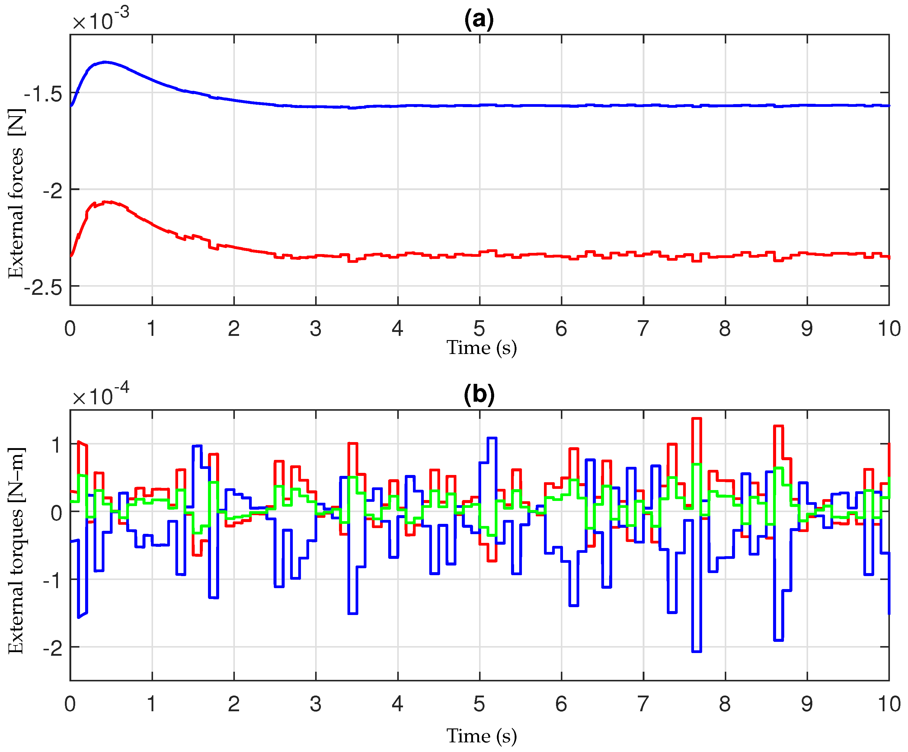
5.1. Environmental Disturbances Acting on the Quadrotor

The principal environmental disturbance acting on the quadrotor is the one applied by the wind. Considering its behavior, wind can be classified into two principal categories: constant wind and turbulent wind. Unfortunately, in many scenarios, the induced speed within a particular wind field is not uniform. For this reason, in our model, variable wind gusts are modeled as lateral wind blasts. These gusts are characterized by their velocity $v_W={(v_{W,X},v_{W,Y})}^T$ in the ground-fixed $(X_E,Y_E)$ frame. The wind velocity components are modeled as

$$\begin{array}{cc}\hfill v_{W,X}& =V_{w}cos({\beta }_0+\Delta {\beta }_0)+0.025N\hfill \\ \hfill v_{W,Y}& =V_{w}sin({\beta }_0+\Delta {\beta }_0)+0.025N\hfill \end{array}$$

where $V_w=V_{w,0}+\Delta V_{w}sin\left({\omega }_w\right)$, with $V_{w,0}$ as the nominal wind magnitude, ${\beta }_0$ is the nominal angle between the $X_E$-axis and the wind vector, and N is a uniform distribution. Additionally, $\Delta {\beta }_0=0.2{\beta }_0$ and $\Delta V_w=0.1V_{w,0}$.

In the vehicle-fixed $(X_B,Y_B)$ frame, the wind velocity components are

$$\begin{array}{cc}\hfill v_{w,x}& =v_{W,X}cos{\alpha }_z+v_{W,Y}sin{\alpha }_z\hfill \\ \hfill v_{w,y}& =-v_{W,X}sin{\alpha }_z+v_{W,Y}cos{\alpha }_z\hfill \end{array}$$

The resulting wind velocity $v_w$ is the sum of the apparent wind velocity $v_x$ due to the vehicle’s forward motion minus $v_{w,x}$ and the apparent wind velocity $v_y$ due to the vehicle’s lateral motion minus $v_{w,y}$, namely $v_{aw,x}=v_x-v_{w,x}$ and $v_{aw,y}=v_y-v_{w,y}$.

Wind gusts induce longitudinal and lateral forces $F_x$ and $F_y$, respectively, as well as roll and yaw moments. The forces and torques due to wind are expressed as

$$\begin{array}{cc}\hfill F_x& =-{\displaystyle \frac{1}{2}}{A}_x\rho C_d{v}_{aw,x}^2\hfill \\ \hfill F_y& =-{\displaystyle \frac{1}{2}}{A}_y\rho C_d{v}_{aw,y}^2\hfill \\ \hfill T_{\varphi }& =-l_{c,z}{F}_y\hfill \\ \hfill T_{\theta }& =-l_{c,z}{F}_x\hfill \\ \hfill T_{\psi }& =l_{c,x}{F}_y-l_{c,y}{F}_x\hfill \end{array}$$

where $A_x$ and $A_y$ represent the vehicle’s front and lateral surfaces, $\rho$ is the air density, $C_d$ is aerodynamic coefficient, and $l_{c,x}$, $l_{c,y}$ are the distances between the center of mass and the center of pressure of each side of the vehicle.

Assumption 4.

For the purposes of this simulation, only the wind components in the x and y directions are considered. This simplification is justified by the following:

 1. 

Lateral wind components (x and y) have a more significant impact on UAV behavior compared to vertical wind components (z).

 2. 

Reducing the model’s complexity facilitates the design and implementation of the controller.

 3. 

Vertical wind components are typically smaller and less perturbative, making this a reasonable and accurate assumption for most UAV operational scenarios.

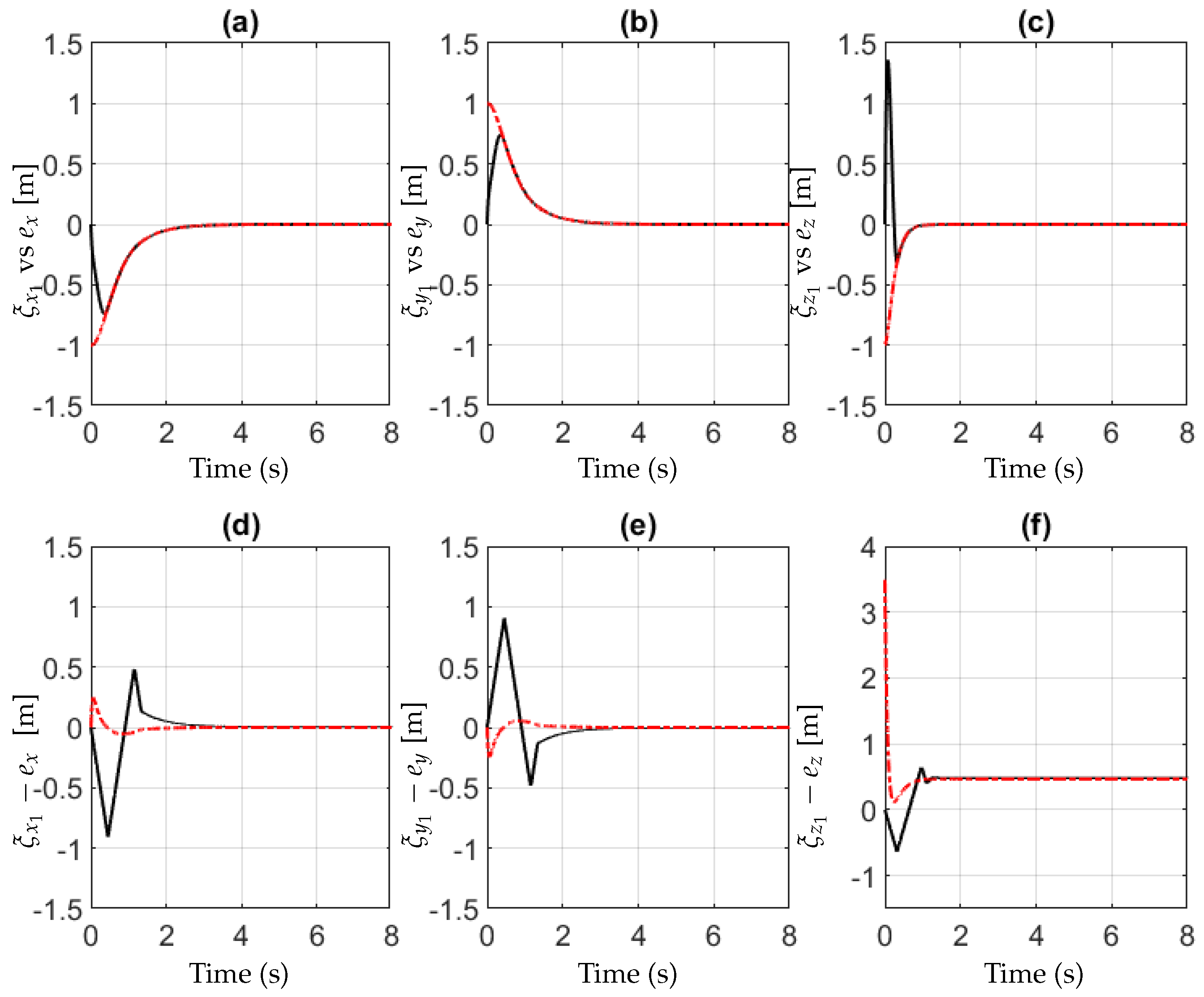
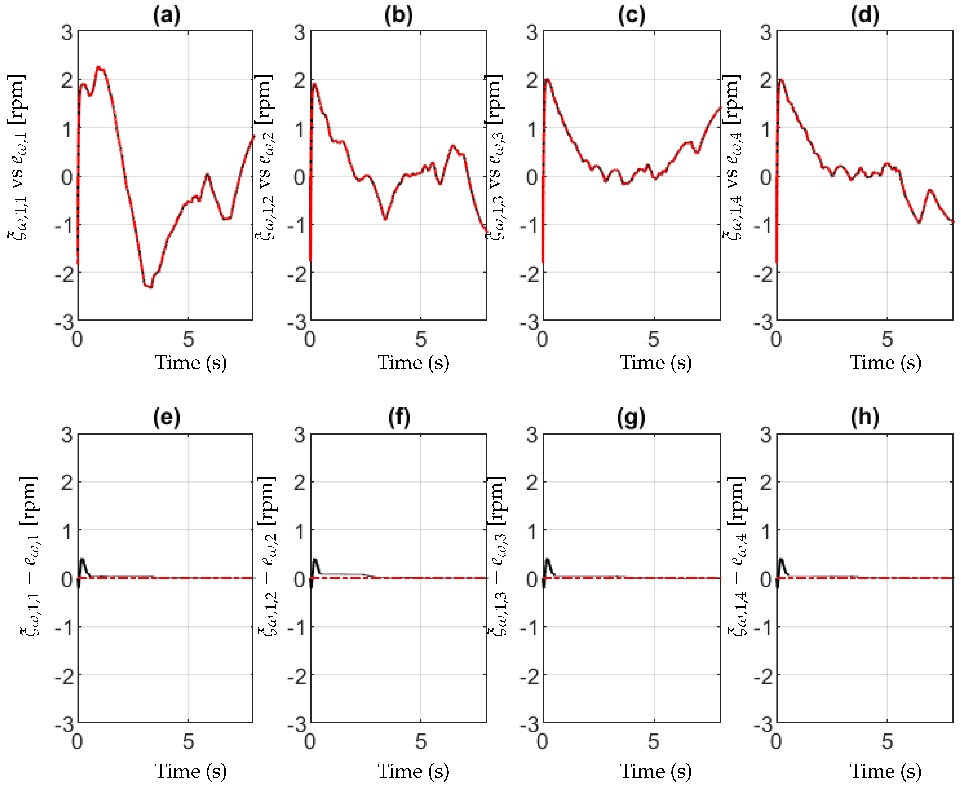
5.2. Simulation Results of Simulink^®

The effectiveness of the suggested control strategy was tested by doing thorough simulations. These simulations were essential for assessing the control system’s performance in different situations and disturbances, guaranteeing its resilience and accuracy in trajectory tracking and stability control.

The performance of the controller has been tested making use of the following references $x_{1,ref}=1$ m, $y_{1,ref}=-1$ m and $z_{1,ref}=1$ m.

The system’s initial conditions for position were initialized as follows: starting at $x_1\left(0\right)=0$ m, $y_1\left(0\right)=0$ m, and $z_1\left(0\right)=0$ m. Velocity had an initial state of $x_2\left(0\right)=0$ m/s, $y_2\left(0\right)=0$ m/s, $z_2\left(0\right)=0$ m/s. As for attitude, the system commenced with ${\varphi }_1\left(0\right)=0$ rad, ${\theta }_1\left(0\right)=0$ rad, and ${\psi }_1\left(0\right)=0$ rad and the rotational velocities in the body frame were initialized at ${\varphi }_2\left(0\right)=0$ rad/s, ${\theta }_2\left(0\right)=0$ rad/s, and ${\psi }_2\left(0\right)=0$ rad/s.

Furthermore, regarding the motors, the initial condition for the current vector was set as $i_i\left(0\right)=0$.

To evaluate the robustness of the system, the following parameter variations had been considered: $m^{\circ }=1.05m$, ${I_{xx}}^{\circ }=1.05I_{xx}$, ${I_{yy}}^{\circ }=1.05I_{yy}$, ${I_{zz}}^{\circ }=1.05I_{zz}$, $K_{m,i}^{\circ }=1.05K_{m,i}$, $B_{m,i}^{\circ }=1.05B_{m,i}$, $J_{m,i}^{\circ }=1.05K_{m,i}$ and $L_i^{\circ }=1.1L_i$.

The control gains for the active control are $k_{x_1}=2$, $k_{y_1}=2$, $k_{z_1}=2$, $k_{x_2}=5$, $k_{y_2}=5$, $k_{z_2}=11$, $k_{d,x_2}=0.5$, $k_{d,y_2}=0.5$, $k_{{\varphi }_1}=35$, $k_{0,{\varphi }_1}=25$, $k_{{\theta }_1}=35$, $k_{0,{\theta }_1}=25$, $k_{{\psi }_1}=5$, $k_{d,{\psi }_1}=0.5$, $k_{{\varphi }_2}=60$, $k_{0,{\varphi }_2}=25$, $k_{{\theta }_2}=60$, $k_{0,{\theta }_2}=25$, $k_{{\psi }_2}=5$, $k_{0,{\psi }_2}=0.5$, ${\lambda }_{x_1}=9$, ${\lambda }_{x_2}=2$, ${\lambda }_{y_1}=9$, ${\lambda }_{y_2}=2$, ${\lambda }_{z_1}=15$, ${\lambda }_{z_2}=2$, ${\lambda }_{{\varphi }_1}=10$, ${\lambda }_{{\varphi }_2}=1$, ${\lambda }_{{\theta }_1}=10$, ${\lambda }_{{\theta }_2}=1$, ${\lambda }_{{\psi }_1}=5$, ${\lambda }_{{\psi }_2}=1$. Concerning the motors, the control gains are: $k_{\omega ,i}=30$ and $k_{i,i}=1$, ${\lambda }_{\omega ,1,i}=10$, ${\lambda }_{\omega ,2,i}=5$, ${\lambda }_{i,1,i}=10$, ${\lambda }_{i,2,i}=15$.

Moreover, the wind behavior is given by a nominal velocity of $V_{w,0}=20$ km/h, a nominal angle of ${\beta }_0=7\pi /4$ rad, and a wind oscillation frequency of ${\omega }_w=0.1$ rad/s. The wind forces exerted on the UAV, along with the torques induced by the wind force, are depicted in Figure 4.

The results are summarized in Figure 5, Figure 6, Figure 7, Figure 8, Figure 9, Figure 10, Figure 11, Figure 12, Figure 13 and Figure 14. Figure 5 shows the quadrotor’s precise positioning illustrated in the three dimensions $x_1$, $y_1$, and $z_1$. The figure marks the initial position of the quadrotor with a green circle at coordinates $(0,0,0)$ and the final position with a red circle at coordinates $(1,-1,1)$. This visualization highlights the path taken by the UAV from its starting point to its target position, providing a clear representation of its movement through space relative to the specified position references $x_{1,ref}$, $y_{1,ref}$, and $z_{1,ref}$. On the other hand, Figure 6a–c portray the quadrotor’s precise positioning in the three dimensions $x_1$, $y_1$, and $z_1$ with respect to their corresponding position references $x_{1,ref}$, $y_{1,ref}$, and $z_{1,ref}$. Simultaneously, Figure 6d–f display the associated tracking errors $e_x$, $e_y$, and $e_z$, providing a visual representation of the outer loop’s performance in the UAV frame. It is evident from these figures that the proposed controller ensures remarkably minimal tracking errors at this outer loop level.

Figure 7 shows the linear velocities $x_2$, $y_2$, and $z_2$ of the UAV over time. Specifically, Figure 7a illustrates the linear velocity $x_2$, Figure 7b depicts the linear velocity $y_2$, and Figure 7c presents the linear velocity $z_2$. These subfigures highlight how the UAV’s linear velocities evolve, providing insights into the system’s dynamic response. Additionally, Figure 7d–f display the tracking errors for these linear velocities, $e_{x_2}$, $e_{y_2}$, and $e_{z_2}$, respectively. These errors represent the difference between the desired and actual velocities, showcasing the controller’s effectiveness in minimizing deviations.

Similarly, Figure 8 presents the orientation dynamics of the UAV. Figure 8a–c show the roll angle ${\varphi }_1$, pitch angle ${\theta }_1$, and yaw angle ${\psi }_1$, respectively, as functions of time. These plots illustrate the UAV’s rotational behavior. Corresponding tracking errors for these angles, $e_{{\varphi }_1}$, $e_{{\theta }_1}$, and $e_{{\psi }_1}$, are depicted in Figure 8d–f. These errors highlight the precision of the attitude control achieved by the proposed system.

Figure 9 shows the angular velocities ${\varphi }_2$, ${\theta }_2$, and ${\psi }_2$ of the UAV. Specifically, Figure 9a illustrates the angular velocity ${\varphi }_2$ in the x-axis, Figure 9b depicts the angular velocity ${\theta }_2$ in the y-axis, and Figure 9c presents the angular velocity ${\psi }_2$ in the z-axis. These subfigures highlight the rotational dynamics and the system’s response. Figure 9d–f display the tracking errors for these angular velocities, $e_{{\varphi }_2}$, $e_{{\theta }_2}$, and $e_{{\psi }_2}$, respectively, showcasing the effectiveness of the inner loop control.

Conversely, Figure 10a–d represent the angular velocities of the quadrotor’s four actuators ${\omega }_1$, ${\omega }_2$, ${\omega }_3$, and ${\omega }_4$ in tandem with their corresponding reference values ${\omega }_{1,ref}$, ${\omega }_{2,ref}$, ${\omega }_{3,ref}$, and ${\omega }_{4,ref}$. Simultaneously, Figure 10e–h illustrate the respective tracking errors for the inner loop of the UAV actuators. The clear results underscore the effectiveness of the proposed controller in achieving minimal tracking errors within this inner loop.

Transitioning to Figure 11a–d, these figures present the current profiles of the quadrotor’s four actuators $i_1$, $i_2$, $i_3$, and $i_4$ alongside their reference values $i_{1,ref}$, $i_{2,ref}$, $i_{3,ref}$, and $i_{4,ref}$. Complementary to this, Figure 11e–h exhibit the corresponding tracking errors.

On the other hand, Figure 12 presents a comprehensive analysis of the estimation process and error dynamics. The subfigures a, b, c, delineate the performance of estimators ${\xi }_{x_1}$, ${\xi }_{y_1}$, and ${\xi }_{z_1}$ in tracking the corresponding errors $e_x$, $e_y$, and $e_z$, providing insights into the estimation precision. Additionally, the variations ${\delta }_{x_1}$, ${\delta }_{y_1}$, and ${\delta }_{z_1}$, tracked by estimators ${\xi }_{x_2}$, ${\xi }_{y_2}$, and ${\xi }_{z_2}$, are portrayed in subfigures d, e, f. This visual representation underscores the effectiveness of the estimation process and its ability to minimize errors while accurately capturing state variations.

Finally, Figure 13 and Figure 14 delve into the inner loop dynamics of the UAV’s actuators, shedding light on the estimation and error characteristics. Figure 13a–d illustrates the performance of estimators ${\xi }_{\omega ,1,1}$, ${\xi }_{\omega ,1,2}$, ${\xi }_{\omega ,1,3}$, and ${\xi }_{\omega ,1,4}$ in tracking the corresponding errors $e_{\omega ,1}$, $e_{\omega ,2}$, $e_{\omega ,3}$, and $e_{\omega ,4}$, while Figure 14a–d showcases the estimators ${\xi }_{i,1,1}$, ${\xi }_{i,1,2}$, ${\xi }_{i,1,3}$, and ${\xi }_{i,1,4}$ monitoring the current associated errors $e_{i,1}$, $e_{i,2}$, $e_{i,3}$, and $e_{i,4}$, offering a comprehensive view of the estimation performance. Furthermore, Figure 13e–h and Figure 14e–h depict the variations ${\delta }_{\omega ,1}$, ${\delta }_{\omega ,2}$, ${\delta }_{\omega ,3}$, ${\delta }_{\omega ,4}$, ${\delta }_{i,1}$, ${\delta }_{i,2}$, ${\delta }_{i,3}$, and ${\delta }_{i,4}$ tracked by estimators. The visual representation collectively underscores the effectiveness of the proposed controller in minimizing errors and accurately estimating the angular velocities and currents within the inner loop.

5.3. Simulation Results of PX4 Autopilot Environment

The “PX4 Autopilot Support from UAV Toolbox” is a comprehensive software tool that facilitates the design, simulation, implementation and validation of flight control algorithms for unmanned aerial vehicles (UAVs) using the PX4 autopilot. Its use focused on verifying and evaluating controller performance in various environments, allowing for extensive validation prior to deployment in real flight conditions.

Therefore, for a direct comparison of the controller’s performance, identical flight references, initial conditions, UAV parameters, parametric variations and external disturbances were maintained, consistent with those utilized in the Simulink^® simulations.

The control gains in this case are: $k_{x_1}=0.5$, $k_{y_1}=0.5$, $k_{z_1}=315$, $k_{0,z_1}=0.014$, $k_{x_2}=222$, $k_{0,z_2}=0.2$, $k_{y_2}=222$, $k_{0,z_2}=0.2$, $k_{z_2}=138$, $k_{0,z_2}=2.15$, $k_{d,z_2}=0.45$, $k_{{\varphi }_1}=30.6$, $k_{{\theta }_1}=30.6$, $k_{{\psi }_1}=115$.

The results are summarized in Figure 15 where, Figure 15a–c portray the quadrotor’s precise positioning in the three dimensions $x_1$, $y_1$, and $z_1$ with respect to their corresponding position references $x_{1,ref}$, $y_{1,ref}$, and $z_{1,ref}$. Simultaneously, Figure 15d–f display the associated tracking errors $e_x$, $e_y$, and $e_z$, providing a visual representation of the outer loop’s performance in the UAV frame. It is evident from these figures that the proposed controller ensures remarkably minimal tracking errors at this outer loop level.

6. Conclusions

Throughout this inquiry, we have designed a complete integrated control system tailored for a UAV equipped with multiple actuators. The main goal was to achieve accurate control over the position reference vector while simultaneously enhancing the controller’s robustness against external disturbances and parameter uncertainties. Numerical simulations were performed using both Simulink® and the simulated PX4 Autopilot environment. The results demonstrated the effectiveness of the proposed control system in achieving precise position control and robust performance for both the UAV and its actuators under various conditions. The control strategy employed two control loops: an outer loop for the UAV frame and an inner loop for the UAV actuators. The outer loop generated the required angular velocities for the actuators to follow the reference position vector, using the UAV’s output. The inner loop ensured that the actuators tracked these angular velocity references. Both control loops utilized PI-like controllers for simplicity. The incorporation of nonlinear control techniques and estimation strategies for disturbances and parameter variations enabled dynamic adaptation to changing environmental conditions. These results underscore the potential applicability of the control system in other UAV operational scenarios.

As part of our future endeavors, we aim to explore the optimization of energy consumption within the system. This includes considering changes to the UAV’s design and architecture, particularly in the context of reconfiguration following the failure of one or more actuators. Investigating the effect of such changes on energy efficiency is consistent with our overarching goal of expanding UAV technologies to not only improve control precision but also address environmental concerns and maximize resource consumption. Additionally, the computational intensity and controller runtime, power consumption, and hardware implementation aspects will be explored in further studies, which are beyond the scope of the current dense article.

References

1. Nex, F.; Armenakis, C.; Cramer, M.; Cucci, D.A.; Gerke, M.; Honkavaara, E.; Kukko, A.; Persello, C.; Skaloud, J. UAV in the advent of the twenties: Where we stand and what is next. ISPRS J. Photogramm. Remote Sens. 2022, 184, 215–242. [Google Scholar] [CrossRef]
2. Sivakumar, M.; Tyj, N.M. A literature survey of unmanned aerial vehicle usage for civil applications. J. Aerosp. Technol. Manag. 2021, 13, e4021. [Google Scholar] [CrossRef]
3. Syed, F.; Gupta, S.K.; Hamood Alsamhi, S.; Rashid, M.; Liu, X. A survey on recent optimal techniques for securing unmanned aerial vehicles applications. Trans. Emerg. Telecommun. Technol. 2021, 32, e4133. [Google Scholar] [CrossRef]
4. Alvares, P.; Silva, L.; Magaia, N. Blockchain-based solutions for UAV-assisted connected vehicle networks in smart cities: A review, open issues, and future perspectives. Telecom 2021, 2, 108–140. [Google Scholar] [CrossRef]
5. Srivastava, A.; Prakash, J. Techniques, answers, and real-world UAV implementations for precision farming. Wirel. Pers. Commun. 2023, 131, 2715–2746. [Google Scholar] [CrossRef]
6. Budiyono, A.; Higashino, S.-I. A review of the latest innovations in UAV technology. J. Instrum. Autom. Syst. 2023, 10, 7–16. [Google Scholar] [CrossRef]
7. Lopez-Sanchez, I.; Moreno-Valenzuela, J. PID control of quadrotor UAVs: A survey. Annu. Rev. Control 2023, 56, 100900. [Google Scholar] [CrossRef]
8. Rinaldi, M.; Primatesta, S.; Guglieri, G. A comparative study for control of quadrotor UAVs. Appl. Sci. 2023, 13, 3464. [Google Scholar] [CrossRef]
9. Maaruf, M.; Mahmoud, M.S.; Ma’arif, A. A survey of control methods for quadrotor UAV. Int. J. Robot. Control Syst. 2022, 2, 652–665. [Google Scholar] [CrossRef]
10. Nguyen, N.P.; Mung, N.X.; Thanh, H.L.N.N.; Huynh, T.T.; Lam, N.T.; Hong, S.K. Adaptive sliding mode control for attitude and altitude system of a quadcopter UAV via neural network. IEEE Access 2021, 9, 40076–40085. [Google Scholar] [CrossRef]
11. Baek, J.; Kang, M. A synthesized sliding-mode control for attitude trajectory tracking of quadrotor UAV systems. IEEE/ASME Trans. Mechatronics 2023, 28, 2189–2199. [Google Scholar] [CrossRef]
12. Shao, X.; Sun, G.; Yao, W.; Liu, J.; Wu, L. Adaptive sliding mode control for quadrotor UAVs with input saturation. IEEE/ASME Trans. Mechatronics 2021, 27, 1498–1509. [Google Scholar] [CrossRef]
13. Noordin, A.; Mohd Basri, M.A.; Mohamed, Z.; Mat Lazim, I. Adaptive PID controller using sliding mode control approaches for quadrotor UAV attitude and position stabilization. Arab. J. Sci. Eng. 2021, 46, 963–981. [Google Scholar] [CrossRef]
14. Koksal, N.; An, H.; Fidan, B. Backstepping-based adaptive control of a quadrotor UAV with guaranteed tracking performance. ISA Trans. 2020, 105, 98–110. [Google Scholar] [CrossRef]
15. Wang, J.; Alattas, K.A.; Bouteraa, Y.; Mofid, O.; Mobayen, S. Adaptive finite-time backstepping control tracker for quadrotor UAV with model uncertainty and external disturbance. Aerosp. Sci. Technol. 2023, 133, 108088. [Google Scholar] [CrossRef]
16. Liu, K.; Wang, R. Antisaturation command filtered backstepping control-based disturbance rejection for a quadarotor UAV. IEEE Trans. Circuits Syst. II Express Briefs 2021, 68, 3577–3581. [Google Scholar] [CrossRef]
17. Bao, C.; Guo, Y.; Luo, L.; Su, G. Design of a fixed-wing UAV controller based on adaptive backstepping sliding mode control method. IEEE Access 2021, 9, 157825–157841. [Google Scholar] [CrossRef]
18. Xu, L.X.; Ma, H.J.; Guo, D.; Xie, A.H.; Song, D.L. Backstepping sliding-mode and cascade active disturbance rejection control for a quadrotor UAV. IEEE/ASME Trans. Mechatronics 2020, 25, 2743–2753. [Google Scholar] [CrossRef]
19. Kazim, M.; Azar, A.T.; Koubaa, A.; Zaidi, A. Disturbance-rejection-based optimized robust adaptive controllers for UAVs. IEEE Syst. J. 2021, 15, 3097–3108. [Google Scholar] [CrossRef]
20. Zhou, L.; Xu, S.; Jin, H.; Jian, H. A hybrid robust adaptive control for a quadrotor UAV via mass observer and robust controller. Adv. Mech. Eng. 2021, 13, 16878140211002723. [Google Scholar] [CrossRef]
21. Wang, J.; Zhu, B.; Zheng, Z. Robust adaptive control for a quadrotor UAV with uncertain aerodynamic parameters. IEEE Trans. Aerosp. Electron. Syst. 2023, 59, 8313–8326. [Google Scholar] [CrossRef]
22. Ristevski, S.; Koru, A.T.; Yucelen, T.; Dogan, K.M.; Muse, J.A. Experimental results of a quadrotor UAV with a model reference adaptive controller in the presence of unmodeled dynamic. In Proceedings of the AIAA Scitech 2022 Forum, San Diego, CA, USA, 3–7 January 2022; p. 1381. [Google Scholar] [CrossRef]
23. García, O.; Ordaz, P.; Santos-Sánchez, O.J.; Salazar, S.; Lozano, R. Backstepping and robust control for a quadrotor in outdoors environments: An experimental approach. IEEE Access 2019, 7, 40636–40648. [Google Scholar] [CrossRef]
24. Islam, S.; Liu, P.X.; El Saddik, A. Robust control of four-rotor unmanned aerial vehicle with disturbance uncertainty. IEEE Trans. Ind. Electron. 2014, 62, 1563–1571. [Google Scholar] [CrossRef]
25. Bianchi, D.; Di Gennaro, S.; Di Ferdinando, M.; Acosta Lúa, C. Robust control of UAV with disturbances and uncertainty estimation. Machines 2023, 11, 352. [Google Scholar] [CrossRef]
26. Xia, K.; Shin, M.; Chung, W.; Kim, M.; Lee, S.; Son, H. Landing a quadrotor UAV on a moving platform with sway motion using robust control. Control Eng. Pract. 2022, 128, 105288. [Google Scholar] [CrossRef]
27. Din, A.F.U.; Mir, I.; Gul, F.; Al Nasar, M.R.; Abualigah, L. Reinforced learning-based robust control design for unmanned aerial vehicle. Arab. J. Sci. Eng. 2023, 48, 1221–1236. [Google Scholar] [CrossRef]
28. Zhao, Z.; Cao, D.; Yang, J.; Wang, H. High-order sliding mode observer-based trajectory tracking control for a quadrotor UAV with uncertain dynamics. Nonlinear Dyn. 2020, 102, 2583–2596. [Google Scholar] [CrossRef]
29. Chandra, A.; Lal, P.P.S. Higher order sliding mode controller for a quadrotor UAV with a suspended load. IFAC-PapersOnLine 2022, 55, 610–615. [Google Scholar] [CrossRef]
30. COMP4DRONES. Agriculture Use Case—COMP4DRONES Project. Available online: https://www.comp4drones.eu/project-info/use-cases/agriculture/ (accessed on 24 June 2024).
31. NASA. UAS Traffic Management (UTM) Project. Available online: https://www.nasa.gov/directorates/armd/past-armd-projects/uas-traffic-management-utm-project/ (accessed on 24 June 2024).
32. Fethalla, N.; Saad, M.; Michalska, H.; Ghommam, J. Robust observer-based dynamic sliding mode controller for a quadrotor UAV. IEEE Access 2018, 6, 45846–45859. [Google Scholar] [CrossRef]
33. Sanwale, J.; Dahiya, S.; Trivedi, P.; Kothari, M. Robust fault-tolerant adaptive integral dynamic sliding mode control using finite-time disturbance observer for coaxial octorotor UAVs. Control Eng. Pract. 2023, 135, 105495. [Google Scholar] [CrossRef]
34. Ha, L.N.N.T.; Hong, S.K. Robust dynamic sliding mode control-based PID–super twisting algorithm and disturbance observer for UAVs. Electronics 2019, 8, 760. [Google Scholar] [CrossRef]
35. Wei, M.; Zheng, L.; Li, H.; Cheng, H. Adaptive Neural Network-based Model Path-Following Contouring Control for Quadrotor Under Diversely Uncertain Disturbances. IEEE Robot. Autom. Lett. 2024. [Google Scholar] [CrossRef]
36. Madebo, M.M.; Abdissa, C.M.; Lemma, L.N.; Negash, D.S. Robust Tracking Control for Quadrotor UAV with External Disturbances and Uncertainties Using Neural Network Based MRAC. IEEE Access 2024, 12, 36183–36201. [Google Scholar] [CrossRef]
37. Verberne, J.; Moncayo, H. Robust control architecture for wind rejection in quadrotors. In Proceedings of the International Conference on Unmanned Aircraft Systems (ICUAS), Atlanta, GA, USA, 11–14 June 2019; pp. 152–161. [Google Scholar] [CrossRef]
38. Wan, K.; Gao, X.; Hu, Z.; Wu, G. Robust motion control for UAV in dynamic uncertain environments using deep reinforcement learning. Remote Sens. 2020, 12, 640. [Google Scholar] [CrossRef]
39. Wan, K.; Li, B.; Gao, X.; Hu, Z.; Yang, Z. A learning-based flexible autonomous motion control method for UAV in dynamic unknown environments. J. Syst. Eng. Electron. 2021, 32, 1490–1508. [Google Scholar] [CrossRef]
40. Mayorga-Macías, W.A.; González-Jiménez, L.E.; Meza-Aguilar, M.A.; Luque-Vega, L.F. Velocity Sensor for Real-Time Backstepping Control of a Multirotor Considering Actuator Dynamics. Sensors 2020, 20, 4229. [Google Scholar] [CrossRef]
41. Wang, B.; Ghamry, K.A.; Zhang, Y. Trajectory tracking and attitude control of an unmanned quadrotor helicopter considering actuator dynamics. In Proceedings of the 2016 35th Chinese Control Conference (CCC), Chengdu, China, 27–29 July 2016; IEEE: New York, NY, USA, 2016; pp. 10795–10800. [Google Scholar] [CrossRef]
42. Di, J.; Kang, Y.; Ji, H.; Wang, X.; Chen, S.; Liao, F.; Li, K. Low-level control with actuator dynamics for multirotor UAVs. Robot. Intell. Autom. 2023, 43, 290–300. [Google Scholar] [CrossRef]
43. Ferry, N. Quadcopter Plant Model and Control System Development with MATLAB/Simulink Implementation. Ph.D. Thesis, Rochester Institute of Technology, Rochester, NY, USA, 2017. Available online: http://www.ritravvenlab.com/uploads/1/1/8/4/118484574/ferry.pdf (accessed on 24 June 2024).
44. Bouabdallah, S. Design and Control of Quadrotors with Application to Autonomous Flying. Ph.D. Thesis, École Polytechnique Fédérale de Lausanne, Lausanne, Switzerland, 2007. Available online: https://infoscience.epfl.ch/record/95939?v=pdf (accessed on 24 June 2024).
45. Mayorga-Macías, W.A. Embedded Control System for a Multi-Rotor Considering Motor Dynamics. Ph.D. Thesis, ITESO—Universidad Jesuita de Guadalajara, San Pedro Tlaquepaque, Mexico, 2020. Available online: https://rei.iteso.mx/items/6cd58f47-b751-4033-ae7f-1d3657d6c258 (accessed on 24 June 2024).
46. ArduPilot Dev Team. Connect ESCs and Motors. Available online: https://ardupilot.org/copter/docs/connect-escs-and-motors.html (accessed on 6 March 2024).
47. Cárdenas R, C.A.; Grisales, V.H.; Collazos Morales, C.A.; Cerón-Muñoz, H.D.; Ariza-Colpas, P.; Caputo-Llanos, R. Quadrotor modeling and a pid control approach. In Proceedings of the Intelligent Human Computer Interaction: 11th International Conference, IHCI 2019, Allahabad, India, 12–14 December 2019; Springer: Berlin/Heidelberg, Germany, 2020; pp. 281–291. [Google Scholar] [CrossRef]
48. Beard, R.W.; McLain, T.W. Small Unmanned Aircraft: Theory and Practice; Princeton University Press: Princeton, NJ, USA, 2024. [Google Scholar]
49. Choi, J.; Cheon, D.; Lee, J. Robust landing control of a quadcopter on a slanted surface. Int. J. Precis. Eng. Manuf. 2021, 22, 1147–1156. [Google Scholar] [CrossRef]
50. Guillén-Bonilla, J.T.; Vaca García, C.C.; Di Gennaro, S.; Sánchez Morales, M.E.; Acosta Lúa, C. Vision-Based Nonlinear Control of Quadrotors Using the Photogrammetric Technique. Math. Probl. Eng. 2020, 2020, 5146291. [Google Scholar] [CrossRef]
51. Acosta Lúa, C.; Vaca García, C.C.; Di Gennaro, S.; Castillo-Toledo, B.; Sánchez Morales, M.E. Real-Time Hovering Control of Unmanned Aerial Vehicles. Math. Probl. Eng. 2020, 2020, 2314356. [Google Scholar] [CrossRef]
52. Schneider, E.E.; Dale, T. Guidelines for Manned Space Flight Experiments; NASA: Washington, DC, USA, 1971. Available online: https://ntrs.nasa.gov/api/citations/19710016459/downloads/19710016459.pdf (accessed on 6 March 2024).
53. Nagaty, A.; Saeedi, S.; Thibault, C.; Seto, M.; Li, H. Control and navigation framework for quadrotor helicopters. J. Intell. Robot. Syst. 2013, 70, 1–12. [Google Scholar] [CrossRef]
54. NASA Glenn Research Center. Drag Equation. Available online: https://www1.grc.nasa.gov/beginners-guide-to-aeronautics/drag-equation/ (accessed on 6 March 2024).
55. Gonzalez-Sierra, J.; Dzul, A.; Martinez, E. Formation control of distance and orientation based-model of an omnidirectional robot and a quadrotor UAV. Robot. Auton. Syst. 2022, 147, 103921. [Google Scholar] [CrossRef]
56. Morbidi, F.; Cano, R.; Lara, D. Minimum-energy path generation for a quadrotor UAV. In Proceedings of the 2016 IEEE International Conference on Robotics and Automation (ICRA), Stockholm, Sweden, 16–21 May 2016; IEEE: New York, NY, USA, 2016; pp. 1492–1498. [Google Scholar]
57. Khalil, H.K. Nonlinear Systems; Prentice Hall: Saddle River, NJ, USA, 2006. [Google Scholar]
58. MathWorks. UAV Toolbox Support Package for PX4 Autopilots. Available online: https://la.mathworks.com/help/uav/px4-spkg.html?s_tid=CRUX_topnav (accessed on 24 June 2024).
Figure 1. Quadrotor schematic.
Drones 08 00447 g001
Figure 2. Brushless DC model.
Drones 08 00447 g002
Figure 3. Robust Control Scheme.
Drones 08 00447 g003
Figure 4. (a) External forces applied by the wind. F x component (red), F y component (blue); (b) External torques applied by the force of the wind. T ϕ (red), T θ (blue), and T ψ (green).
Drones 08 00447 g004
Figure 5. Three-dimensional trajectory of the UAV showing the initial point (green circle) at ( 0 , 0 , 0 ) and the final point (red circle) at ( 1 , 1 , 1 ) .
Drones 08 00447 g005
Figure 6. (a) Position x 1 (black) and reference x 1 , r e f (red dash–dot line); (b) position y 1 (black) and reference y 1 , r e f (red dash–dot line); (c) position z 1 (black) and reference y 1 , r e f (red dash–dot line); (d) tracking error e x = x 1 x 1 , r e f ; (e) tracking error e y = y 1 y 1 , r e f ; (f) tracking error e z = z 1 z 1 , r e f .
Drones 08 00447 g006
Figure 7. (a) Linear velocity x 2 ; (b) linear velocity y 2 ; (c) linear velocity z 2 ; (d) tracking error e x 2 = x 2 x 2 , d ; (e) tracking error e y 2 = y 2 y 2 , d ; (f) tracking error e z 2 = z 2 z 2 , d .
Drones 08 00447 g007
Figure 8. (a) Roll ϕ 1 ; (b) pitch θ 1 ; (c) yaw ψ 1 ; (d) tracking error e ϕ 1 = sin ϕ 1 sin ϕ 1 , d ; (e) tracking error e θ 1 = sin θ 1 sin θ 1 , d ; (f) tracking error e ψ 1 = ψ 1 ψ 1 , r e f .
Drones 08 00447 g008
Figure 9. (a) Angular velocity in x, ϕ 2 ; (b) angular velocity in y, θ 2 ; (c) angular velocity in z, ψ 2 ; (d) tracking error e ϕ 2 = ϕ 2 ϕ 2 , d ; (e) tracking error e θ 2 = θ 2 θ 2 , d ; (f) tracking error e ψ 2 = ψ 2 ψ 2 , d .
Drones 08 00447 g009
Figure 10. (a) Angular velocity ω 1 (black) and reference ω 1 , r e f (red dash–dot line); (b) angular velocity ω 2 (black) and reference ω 2 , r e f (red dash–dot line); (c) angular velocity ω 3 (black) and reference ω 3 , r e f (red dash–dot line); (d) angular velocity ω 4 (black) and reference ω 4 , r e f (red dash–dot line); (e) tracking error e ω 1 = ω 1 ω 1 , r e f ; (f) tracking error e ω 2 = ω 2 ω 2 , r e f ; (g) tracking error e ω 3 = ω 3 ω 3 , r e f ; (h) tracking error e ω 4 = ω 4 ω 4 , r e f .
Drones 08 00447 g010
Figure 11. (a) Current i 1 (black) and reference i 1 , r e f (red dash–dot line); (b) current i 2 (black) and reference i 2 , r e f (red dash–dot line); (c) current i 3 (black) and reference i 3 , r e f (red dash–dot line); (d) current i 4 (black) and reference i 4 , r e f (red dash–dot line); (e) tracking error e i 1 = i 1 i 1 , r e f ; (f) tracking error e i 2 = i 2 i 2 , r e f ; (g) tracking error e i 3 = i 3 i 3 , r e f ; (h) tracking error e i 4 = i 4 i 4 , r e f .
Drones 08 00447 g011
Figure 12. (a) Estimator ξ x 1 (black) and error e x (red dash–dot line); (b) estimator ξ y 1 (black) and error e y (red dash–dot line); (c) estimator ξ z 1 (black) and error e z (red dash–dot line); (d) estimator ξ x 2 (black) and variation δ x 1 (red dash–dot line); (e) estimator ξ y 2 (black) and variation δ y 1 (red dash–dot line); (f) estimator ξ z 2 (black) and variation δ z 1 (red dash–dot line).
Drones 08 00447 g012
Figure 13. (a) Estimator ξ ω , 1 , 1 (black) and error e ω , 1 (red dash–dot line); (b) estimator ξ ω , 1 , 2 (black) and error e ω , 2 (red dash–dot line); (c) estimator ξ ω , 1 , 3 (black) and error e ω , 3 (red dash–dot line); (d) estimator ξ ω , 1 , 4 (black) and error e ω , 4 (red dash–dot line); (e) estimator ξ ω , 2 , 1 (black) and variation δ ω , 1 (red dash–dot line); (f) estimator ξ ω , 2 , 2 (black) and variation δ ω , 2 (red dash–dot line); (g) estimator ξ ω , 2 , 3 (black) and variation δ ω , 3 (red dash–dot line); (h) estimator ξ ω , 2 , 4 (black) and variation δ ω , 4 (red dash–dot line).
Drones 08 00447 g013
Figure 14. (a) Estimator ξ i , 1 , 1 (black) and error e i , 1 (red dash–dot line); (b) estimator ξ i , 1 , 2 (black) and error e i , 2 (red dash–dot line); (c) estimator ξ i , 1 , 3 (black) and error e i , 3 (red dash–dot line); (d) estimator ξ i , 1 , 4 (black) and error e ω , 4 (red dash–dot line); (e) estimator ξ i , 2 , 1 (black) and variation δ i , 1 (red dash–dot line); (f) estimator ξ i , 2 , 2 (black) and variation δ i , 2 (red dash–dot line); (g) estimator ξ i , 2 , 3 (black) and variation δ i , 3 (red dash–dot line); (h) estimator ξ i , 2 , 4 (black) and variation δ i , 4 (red dash–dot line).
Drones 08 00447 g014
Figure 15. (a) Position x 1 (black) and reference x 1 , r e f (red dash–dot line); (b) position y 1 (black) and reference y 1 , r e f (red dash–dot line); (c) position z 1 (black) and reference y 1 , r e f (red dash–dot line); (d) tracking error e x = x 1 x 1 , r e f ; (e) tracking error e y = y 1 y 1 , r e f ; (f) tracking error e z = z 1 z 1 , r e f .
Drones 08 00447 g015
Disclaimer/Publisher’s Note: The statements, opinions and data contained in all publications are solely those of the individual author(s) and contributor(s) and not of MDPI and/or the editor(s). MDPI and/or the editor(s) disclaim responsibility for any injury to people or property resulting from any ideas, methods, instructions or products referred to in the content.