Fixed-Time Fault-Tolerant Adaptive Neural Network Control for a Twin-Rotor UAV System with Sensor Faults and Disturbances

Abstract

This paper presents a fixed-time fault-tolerant adaptive neural network control scheme for the Twin-Rotor Multi-Input Multi-Output System (TRMS), which is challenging due to its complex, unstable dynamics and helicopter-like behavior with two degrees of freedom (DOFs). The control objective is to stabilize the TRMS in trajectory tracking in the presence of unknown nonlinear dynamics, external disturbances, and sensor faults. The proposed approach employs the backstepping technique combined with adaptive neural network estimators to achieve fixed-time convergence. The unknown nonlinear functions and disturbances of the system are processed via an adaptive radial basis function neural network (RBFNN), while the sensor faults are actively estimated using robust terms. The developed controller is applied to the TRMS using a decentralized structure where each DOF is controlled independently to simplify the control scheme. Moreover, the parameters of the proposed controller are optimized by the gray-wolf optimization algorithm to ensure high flight performance. The system’s stability analysis is proven using a Lyapunov approach, and simulation results demonstrate the effectiveness of the proposed controller.

1. Introduction

In recent years, the field of automatic control engineering has seen remarkable progress in the study and implementation of autonomous aerial vehicles (UAVs) [1]. These developments have provided unprecedented efficiency and sustainability for a variety of civil and military applications. However, controlling these vehicles poses significant challenges due to their complex dynamics, requiring solutions for nonlinearities, system uncertainties, external disturbances, and sensor faults. Ensuring their safety and reliability is of paramount importance, especially given their potential applications. UAV helicopters with rotors are among the most reliable drones on the market today thanks to their engineering redundancy.

As control systems become more complex, ensuring their security remains crucial. Developing control theories capable of handling system faults is essential. Fault diagnosis and fault-tolerant control (FTC) are key challenges in modern control theory. The primary objective is to design control laws that maintain stability and performance despite faults in sensors or actuators, ensuring robustness by mitigating their adverse effects.

1.1. Related Works

In current research, FTC techniques are generally categorized as either passive or active, as indicated in [2,3,4]. Passive FTC (PFTC) systems employ a single controller with a fixed structure and parameters to manage all predefined failure scenarios without necessitating online fault detection, diagnosis, or control reconfiguration. While this approach is easier to implement, it tends to be more conservative and less adaptive to unexpected faults. Several PFTC approaches have been introduced [5,6,7,8,9,10,11,12], each aiming to enhance the robustness and reliability of control systems under various fault conditions. In [6,10,11], the authors proposed an adaptive passive FTC method based on sliding-mode control. The backstepping technique was suggested in [5] for dealing with quadrotor propeller failures. Additionally, the combination of intelligent approaches using fuzzy and/or neural networks has proven highly effective in estimating unknown fault functions, as demonstrated in [7,12,13].

However, unexpected failures can compromise the stability and effectiveness of the control system, which passive approaches cannot guarantee. This shortcoming underscores the necessity for developing innovative methods and control strategies specifically designed for active FTC systems as demonstrated in [14,15,16,17].

1.2. Research Motivation

Despite demonstrating suitable results and contributing to addressing several problems in system control, especially in the UAV domain, the aforementioned works have certain limitations. These approaches often rely on ideal knowledge and precise modeling of the system, which is not always feasible. In many cases, the design of the controller is closely tied to an accurate system model, which may not account for nonlinearities, disturbances, and uncertainties. To overcome these challenges, several works have been introduced that consider the system model subject to such complexities, treating it as an unknown model [18,19,20]. These models can be estimated based on various approaches, allowing for a more robust and adaptive control strategy.

The step-by-step methodology of backstepping enables a modular design approach, as demonstrated [13,21], which showed promising results. In this approach, complex systems can be broken down into simpler subsystems, with each subsystem designed and analyzed individually before integrating them into the overall control scheme. Furthermore, backstepping can be extended to include adaptive control mechanisms, enabling the estimation of unknown values in the dynamic system, with or without fault estimation. This adaptability is crucial for enhancing system robustness and maintaining reliable performance despite the existence of uncertainties and faults. Motivated by the above-mentioned works, we aim to develop a controller that does not rely on prior knowledge of the dynamic model and can handle sensor failures. This approach is applied to the Twin-Rotor Multi-Input Multi-Output System (TRMS) [22], which represents a helicopter-like UAV with two degrees of freedom (DOFs), where each DOF describes the flight dynamics in the vertical and horizontal planes.

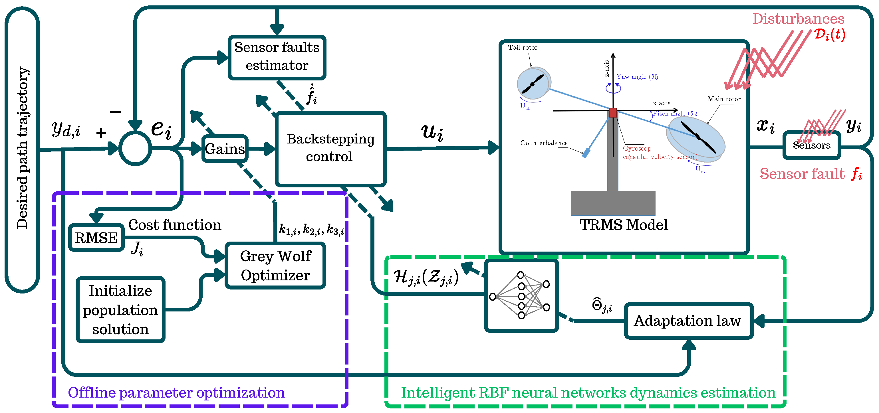
1.3. Proposed Methodology and Contributions

In this paper, we propose a novel active FTC strategy for the TRMS to enhance its reference tracking performance in the presence of unknown dynamics, disturbances, and sensor faults. Our control scheme is designed using the backstepping technique combined with adaptive neural network estimators, ensuring fixed-time stabilization of the closed-loop system. Given that the TRMS is a multi-variable system, we implement the control through a decentralized structure, applying the proposed approach to each input separately. The control law developed in this work leverages a series of virtual inputs that use sensor fault estimators and an adaptive RBFNN to manage the unknown nonlinear dynamics and disturbances. Additionally, to optimize the selection of control parameters, we employ the gray-wolf optimization (GWO) algorithm, which has demonstrated strong convergence to both local and global solutions compared to other metaheuristic algorithms, as shown in [23,24]. Furthermore, GWO has proven its flexibility in parameter tuning across various applications, as highlighted in [25,26]. This paper’s primary contributions can be summarized as follows:

• A novel fault-tolerant control strategy for the TRMS that ensures stability and robust tracking performance is proposed. Our approach utilizes a backstepping technique combined with an RBFNN adaptive estimator. By employing this method, we can guarantee robust control performance while maintaining accurate tracking of desired trajectories.
• The issue of sensor faults in the control system is addressed by incorporating active fault-tolerant control techniques, which ensure the system’s resilience in the presence of these faults and preserve reliable flight operations.
• To guarantee the stability of the entire closed-loop system, we employ Lyapunov’s theorem, which offers mathematical proof of fixed-time stability. Hence, fixed-time stabilization provides a robust and efficient solution for flight systems facing disturbances and sensor faults, ensuring rapid responses, stable performance, and enhanced safety.
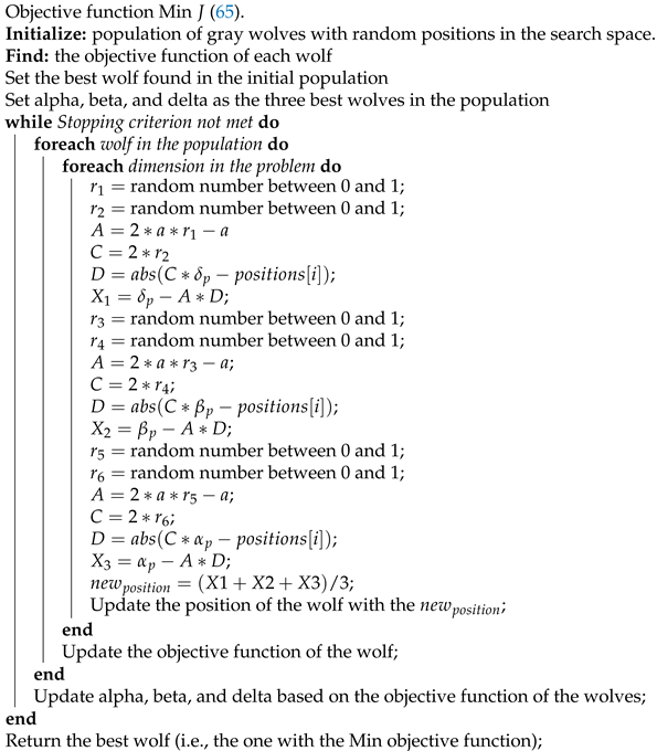
• To identify the best control parameter values and address the selection problem, we introduce a metaheuristic optimization algorithm based on GWO. This algorithm allows us to automatically select the optimal design and improves the performance of the TRMS.

Therefore, the major advantages of the proposed approach in control design compared to existing methods can be summarized as follows:

i.

Unlike classical controllers [27,28], which depend on accurate system modeling and extensive tuning, the proposed controller is model-free and does not require a detailed model. This flexibility allows it to better handle uncertainties and dynamic changes, providing more robust and reliable performance across various scenarios.

ii.

Unlike the approaches in [29,30], which focus on algebraic methods, our controller incorporates fixed-time stability guarantees. This ensures that the system’s stability is achieved within a finite time frame, regardless of initial conditions or disturbances, providing superior robustness and reliability compared to algebraic methods that may not account for time-dependent stability.

iii.

Unlike [13,31], who employ a separate neural network for each unknown nonlinear function, our proposed design uses a single neural network for each subsystem. This streamlined approach significantly reduces computational complexity and simplifies implementation, offering a more efficient and manageable control system design.

iv.

Our proposed active fault-tolerant control structure integrates fault estimation and compensation directly, unlike the approaches in [32,33], which require a separate observer for these tasks. This integrated design simplifies the control system and improves overall efficiency by eliminating the need for an additional observer.

The rest of this paper is organized as follows. Section 2 discusses the preliminaries of fixed-time stability and the RBFNN approximation, together with the formulation of the TRMS with sensor faults. Section 3 provides the detailed design procedure for the fixed-time adaptive neural controller, as well as the active fault-tolerant control and the optimization algorithm. Section 4 presents the numerical results that highlight the effectiveness of the proposed control scheme. Finally, this study’s conclusions and recommendations for further research are provided in Section 5.

2. Foundational Concepts and Model Formulation

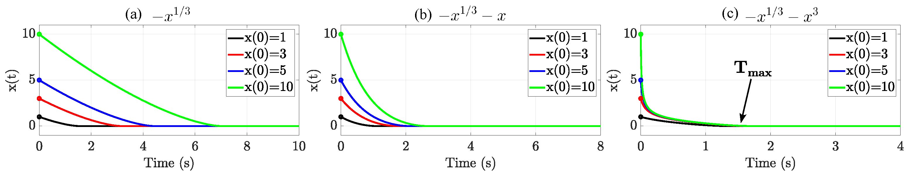
2.1. Essential Preliminaries: Fixed-Time Stability and Radial Basis Function Neural Networks

Fixed-time stability refers to a system property where the system’s state trajectory stabilizes to the equilibrium point within a fixed, pre-specified time, regardless of the initial conditions. This contrasts with finite-time stability, where the settling time depends on the initial conditions. The property of fixed-time convergence is particularly beneficial for systems where stability needs to be guaranteed within a certain time frame, regardless of the initial conditions.

Consider the nonlinear system described by

$$\dot{x}=f(t,x\left(t\right)),x\left(0\right)=x_0$$

(1)

where $x\in \mathbb{R}$ and $f:{\mathbb{R}}^{+}\times {\mathbb{R}}^n\to {\mathbb{R}}^n$ is a nonlinear function. The equilibrium of system (1) is said to be semi-globally practically fixed-time stable (SGPF-TS) if, for any initial condition $x\left(0\right)\in \mathsf{\Omega }$, there exists a solution such that $\parallel x(t,x_0)\parallel \le \epsilon$, which converges to the equilibrium in bounded finite time $T\left(x_0\right)$, i.e., $\exists T_{max}>0:T\left(x_0\right)\le T_{max},\forall x_0\in \mathsf{\Omega }$. As demonstrated in Figure 1.

The solutions of the system in Figure 1a, approach the origin at some finite-time moment, making the system finite-time stable as a result of the fractional power 1/3. However, the convergence is still slow as long as the state is far from 1, which leads us to the second system in Figure 1b. Because of the term $-x\left(t\right)$, the system can achieve fast convergence for any initial state $x_0$. In the system in Figure 1c, where there is one fractional exponent greater than 1, fast convergence is achieved, and the settling time is bounded from above by a constant $T_{max}$ that can be estimated independently of the initial conditions.

Lemma 1 

([34]). Let $\alpha ,\beta >0,p>1,$ and $0<q<1$ be design constants such that

$$\dot{\mathcal{L}}\le -\alpha {\mathcal{L}}^p\left(x\right)-\beta {\mathcal{L}}^q\left(x\right)$$

(2)

where $\mathcal{L}\left(x\right)$ is the Lyapunov function. The origin of (1) is stable in fixed time with the settling time T that can be predicted by

$$T\le T_{max}:={\displaystyle \frac{1}{\alpha (p-1)}}+{\displaystyle \frac{1}{\beta (1-q)}}$$

(3)

Lemma 2 

([35]). Let $\alpha ,\beta >0,p>1,0<q<1,$ and $0<\eta <\infty$ be design constants such that

$$\dot{\mathcal{L}}\le -\alpha {\mathcal{L}}^p\left(x\right)-\beta {\mathcal{L}}^q\left(x\right)+\eta$$

(4)

The trajectory of (1) is practically fixed-time stable, and the settling time function T can be determined by

$$T\le T_{max}:={\displaystyle \frac{1}{\alpha \phi (p-1)}}+{\displaystyle \frac{1}{\beta \phi (1-q)}}$$

(5)

with the positive constant $0<\phi <1$. The residual set solution of system (1) is given by

$$\left.x\in \left\{\mathcal{L}\left(x\right)\le min{\left\{{\left({\displaystyle \frac{\eta }{(1-\phi )\alpha }}\right)}^{{\displaystyle \frac{1}{p}}},{\displaystyle \frac{\eta }{(1-\phi )\beta }}\right)}^{{\displaystyle \frac{1}{q}}}\right\}\right\}$$

(6)

Lemma 3. 

Let $b_1,b_2$, and $b_3$ be arbitrary positive constants. Then, the following inequality holds:

$${\left|x\right|}^{b_1}{\left|y\right|}^{b_2}\le {\displaystyle \frac{b_1}{b_1+b_2}}{b}_3{\left|x\right|}^{b_1+b_2}+{\displaystyle \frac{b_2}{b_1+b_2}}{b}_3^{-{\displaystyle \frac{b_1}{b_2}}}{\left|y\right|}^{b_1+b_2}$$

(7)

for any real variables x and y.

Lemma 4 

([36,37]). For any nonlinear unknown function $\mathcal{H}\left(\mathcal{Z}\right)$ and the compact set $C_{\mathcal{Z}}$ , there exists an RBFNN satisfying

$$\mathcal{H}\left(\mathcal{Z}\right)={\mathcal{W}}^T\mathsf{\Phi }\left(\mathcal{Z}\right)+\delta \left(\mathcal{Z}\right)$$

(8)

where $\mathcal{W}=[{\omega }_1,{\omega }_2,\dots ,{\omega }_l]\in {\mathbb{R}}^l$ represents the NN ideal weights; l is the number of NN nodes; $\mathsf{\Phi }\left(\mathcal{Z}\right)={[{\mathsf{\Phi }}_1\left(\mathcal{Z}\right),\dots ,{\mathsf{\Phi }}_l\left(\mathcal{Z}\right)]}^T\in {\mathbb{R}}^l$ represents the radial basis function (RBF) vector selected as ${\mathsf{\Phi }}_i\left(\mathcal{Z}\right)=exp(-\parallel \mathcal{Z}-{\mu }_i{\parallel }^2/{\eta }^2)$; ${\mu }_i$ and η denote the center and the width of the RBF, respectively; and finally, $\delta \left(\mathcal{Z}\right)$ represents the approximation error, which is bounded by $\delta \left(\mathcal{Z}\right)$, i.e., $\left|\delta \right(\mathcal{Z}\left)\right|\le \epsilon ,\epsilon >0.$

The optimal weights ${\mathcal{W}}^{*}$ minimizing the network approximation errors ε are given by

$${\mathcal{W}}^{*}=\underset{\mathcal{W}\in R^l}{argmin}\{\underset{\mathcal{Z}\in {\mathsf{\Omega }}_{\mathcal{Z}}}{sup}|f\left(\mathcal{Z}\right)-{\mathcal{W}}^T\mathsf{\Phi }\left(\mathcal{Z}\right)\left|\right\}$$

(9)

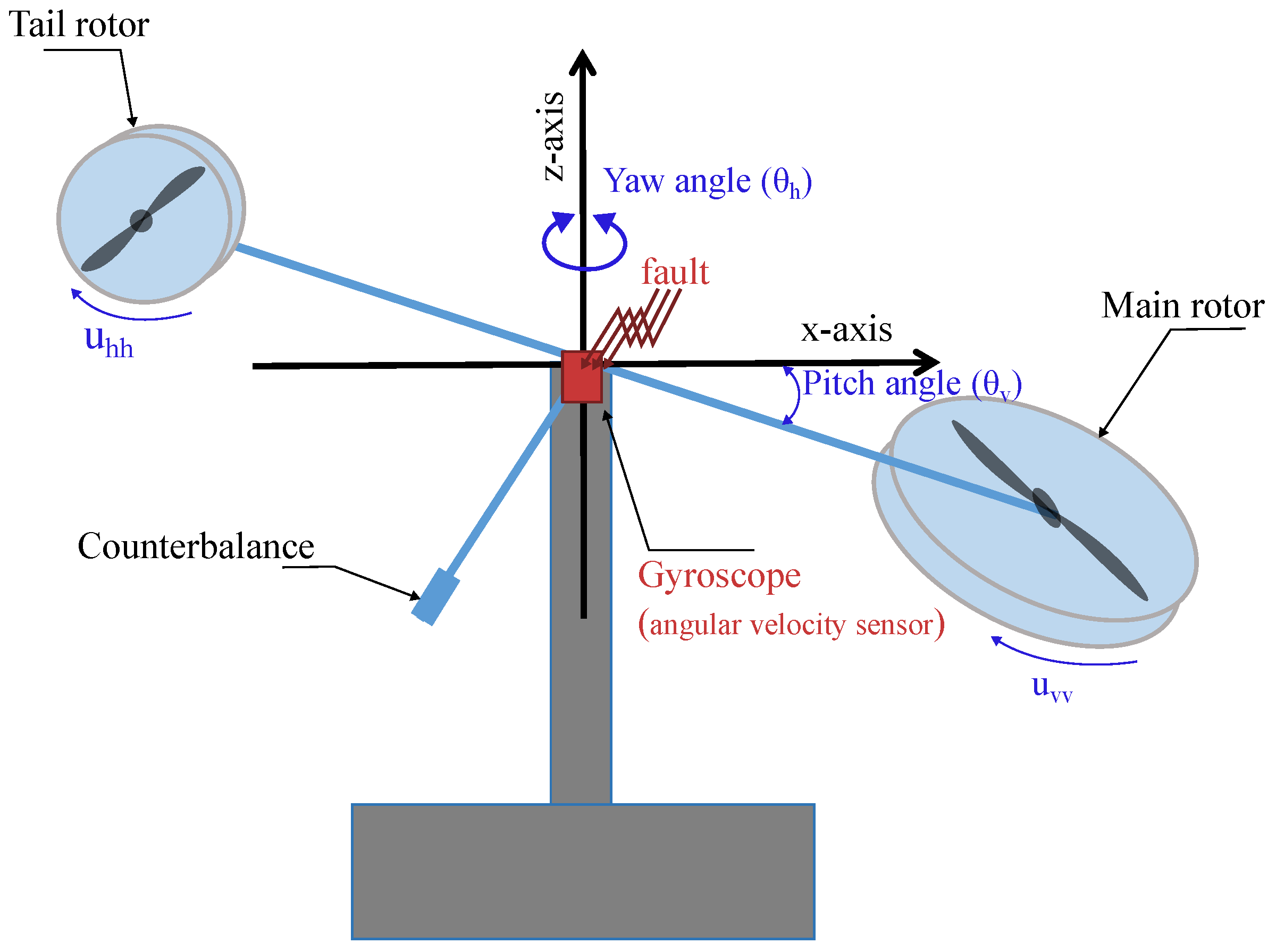
2.2. Twin-Rotor MIMO System: Description and Dynamic Modeling

The TRMS offers a significant opportunity for exploring control theory and systems engineering due to its complex and highly coupled dynamics. Designed to emulate the challenging dynamics of a helicopter, the TRMS offers a practical platform for developing and testing control strategies for real-world applications. The system is composed of two rotors affixed to a beam that can execute pitch and yaw movements around its central axis, as shown in Figure 2. While the main rotor governs the pitch motion, the tail rotor affects the yaw motion. Control over these motions is facilitated through the adjustment of the input voltage of each rotor. The complexity of the TRMS dynamics stems from the nonlinearity and the strong coupling effect between the pitch and yaw motions. Moreover, the system can be influenced by parameter uncertainties, external disturbances, and sensor faults, which further complicate its control.

The nonlinear model of the TRMS is elaborated to describe the flight dynamics in the vertical and horizontal planes. During its motion, the positions of the main and tail rotors are determined by two angles: the pitch angle ${\theta }_v$ and the yaw angle ${\theta }_h$, respectively. From the literature [22], the mathematical model describing the dynamics of the TRMS in both planes is given by

$$\left\{\begin{array}{cc}& {\dot{\theta }}_v={\mathsf{\Omega }}_v\hfill \\ & J_v{\dot{\mathsf{\Omega }}}_v=(a_m{u}_{vv}^2+b_m{u}_{vv})(1-K_{gy}{\mathsf{\Omega }}_{h}cos\left({\theta }_v\right))\hfill \\ & -M_{g}sin{\theta }_v-B_v{\mathsf{\Omega }}_v+K_{gx}{\mathsf{\Omega }}_h^{2}sin\left(2{\theta }_v\right)+d_v\left(t\right)\hfill \\ & T_{m_1}{\dot{u}}_{vv}=-T_{m_0}{u}_{vv}+k_m{u}_v\hfill \end{array}\right.$$

(10)

$$\left\{\begin{array}{cc}& {\dot{\theta }}_h={\mathsf{\Omega }}_h\hfill \\ & J_h{\dot{\mathsf{\Omega }}}_h=a_t{u}_{hh}^2+b_t{u}_{hh}-B_h{\mathsf{\Omega }}_h-M_R+d_h\left(t\right)\hfill \\ & T_{t_1}{\dot{u}}_{hh}=-T_{t_0}{u}_{hh}+k_t{u}_h\hfill \end{array}\right.$$

(11)

where ${\mathsf{\Omega }}_v$ and ${\mathsf{\Omega }}_h$ are the angular velocities; $u_{vv}$ and $u_{hh}$ are the momentum of the main and tail DC motors, respectively, and are assumed to be measurable; $u_v$ and $u_h$ are the control inputs; and $d_v$ and $d_h$ are the external disturbances that satisfy $d_v\le d_{0,v}$ and $d_h\le d_{0,h}$, respectively, with unknown upper bounds $d_{0,v}$ and $d_{0,h}$. $M_R$ is the cross-reaction momentum expressed by

$$M_R={\displaystyle \frac{k_c(T_{0}s+1)}{T_{p}s+1}}(a_t{u}_{hh}^2+b_t{u}_{hh})$$

(12)

which can be written in the time domain as [38]

$$M_R=0.375k_c{e}^{-0.5t}(a_t{u}_{hh}^2+b_t{u}_{hh})$$

(13)

The remaining parameters and constants, along with their numerical values, can be found in [22].

The previous model describes the dynamic and functional characteristics of the TRMS and is given in this paper only for simulation purposes. The representations (10) and (11) can be written in a decoupled form, representing the motion in the vertical and horizontal planes. This simplification helps in the design process of the proposed controller by treating the pitch and yaw subsystems as independent entities. The decoupled model is presented as follows:

$$\left\{\begin{array}{cc}& {\dot{\theta }}_v={\mathsf{\Omega }}_v\hfill \\ & J_v{\dot{\mathsf{\Omega }}}_v=a_m{u}_{vv}^2+b_m{u}_{vv}-M_{g}sin{\theta }_v-B_v{\mathsf{\Omega }}_v+{\mathcal{D}}_v\hfill \\ & T_{m_1}{\dot{u}}_{vv}=-T_{m_0}{u}_{vv}+k_m{u}_v\hfill \end{array}\right.$$

(14)

$$\left\{\begin{array}{cc}& {\dot{\theta }}_h={\mathsf{\Omega }}_h\hfill \\ & J_h{\dot{\mathsf{\Omega }}}_h=a_t{u}_{hh}^2+b_t{u}_{hh}-B_h{\mathsf{\Omega }}_h+{\mathcal{D}}_h\hfill \\ & T_{t_1}{\dot{u}}_{hh}=-T_{t_0}{u}_{hh}+k_t{u}_h\hfill \end{array}\right.$$

(15)

with ${\mathcal{D}}_v=-(a_m{u}_{vv}^2+b_m{u}_{vv})K_{gy}{\mathsf{\Omega }}_{h}cos\left({\theta }_v\right))+K_{gx}{\mathsf{\Omega }}_h^{2}sin\left(2{\theta }_v\right)+d_v\left(t\right)$ and ${\mathcal{D}}_h=-M_R+d_h\left(t\right)$ grouping the effects of the cross-reaction moment between rotors, the gyroscopic moment, and external disturbances.

Considering the angular velocity sensor faults, i.e., faults in the gyroscope system, with the notations $x_v={[x_{1,v},x_{2,v},x_{3,v}]}^T={[{\theta }_v,{\mathsf{\Omega }}_v,u_{v}v]}^T$ and $x_h={[x_{1,h},x_{2,h},x_{3,h}]}^T={[{\theta }_h,{\mathsf{\Omega }}_h,u_h]}^T$, the state variables of the TRMS with sensor faults, which are assumed to be measurable, are represented as follows:

$$\left\{\begin{array}{cc}& y_{1,i}=x_{1,i}\hfill \\ & y_{2,i}=f_{m,i}{x}_{2,i}\left(t\right)+f_{a,i}\hfill \\ & y_{3,i}=x_{3,i}\hfill \end{array}\right.$$

(16)

where $y_i={[y_{1,i},y_{2,i},y_{3,i}]}^T$ for $i\in \{h,v\}$ represents the measured state vector of the TRMS in the horizontal and vertical planes; $f_{a,i}$ denotes the additive fault represented by bias, drift, and loss of accuracy; and $f_{m,i}$ denotes the multiplicative faults represented by the sensor loss of effectiveness. Thus, only the faulted states are available for the controller and are described below.

Bias:

A constant offset added to the sensor output.

$$y_{2,i}=x_{2,i}\left(t\right)+f_{a,i}$$

(17)

with ${\dot{f}}_{a,i}\equiv 0$ and $f_{a,i}\left(t_f\right)\ne 0$

Drift:

A slow change over time, typically linear, added to the sensor output.

$$y_{2,i}=x_{2,i}\left(t\right)+f_{a,i}\left(t\right)$$

(18)

with $|f_{a,i}\left(t\right)|=d_{i}t$ and $0<d_i\ll 1$ for all $t\ge t_f$

Loss of accuracy:

Random fluctuations added to the sensor output.

$$y_{2,i}=x_{2,i}\left(t\right)+f_{a,i}\left(t\right)$$

(19)

with $|f_{a,i}|<f_{a0,i}$ and ${\dot{f}}_{a,i}arrow0$ for all $t\le t_f$

Loss of effectiveness:

A scaling down of the sensor output.

$$y_{2,i}=f_{m,i}\left(t\right)x_{2,i}\left(t\right)$$

(20)

with $0<f_{m0,i}\le f_{m,i}\le 1$ for all $t\ge t_f$, where $t_f$ is the time instant of failure, and $f_{a,i}$ and $f_{m,i}$ are smoothly varying within [−$f_{a0,i}$,$f_{a0,i}$] and [$f_{m0,i}$,1].

With a few adjustments, (16) can be rearranged as

$$y_{2,i}\left(t\right)=x_{2,i}\left(t\right)+f_i(t,x_{2,i})$$

(21)

where $f_i(t,x_{2,i})=(f_{m,i}\left(t\right)-1)x_{2,i}\left(t\right)+f_{a,i}\left(t\right)$ represents an equivalent sensor fault that includes all the types mentioned above.

$$\left\{\begin{array}{c}{\dot{y}}_{1,i}=y_{2,i}-f_i\hfill \\ {\dot{y}}_{2,i}=y_{3,i}+{\alpha }_i\left(x\right)+{\mathcal{D}}_i\left(t\right)+{\dot{f}}_i\hfill \\ {\dot{y}}_{3,i}=u_i+{\beta }_i\left(x\right)\hfill \end{array}\right.$$

(22)

where ${\alpha }_i\left(x\right)$ and ${\beta }_i\left(x\right)$ denote unknown nonlinear functions that represent the dynamics of the system. These functions are estimated using an RBFNN.

The objective is to design an adaptive control law with updating laws so that the twin-rotor system outputs $y_i$ track the desired reference signals $y_{d,i}$ in fixed time and compensate for disturbances and sensor faults. The control system aims to accurately regulate the TRMS’s pitch and yaw angles despite the occurrence of various sensor faults, such as additive and multiplicative faults. By employing a backstepping control technique, complemented by a radial basis function neural network (RBFNN) for approximating unknown system dynamics, we aim to achieve robust control performance, fixed-time stability, and fault tolerance, thereby enhancing the system’s resilience to disturbances and uncertainties.

3. Control Design

This section provides the design of a fault-tolerant fixed-time adaptive neural controller (FTFxTAC) for the pitch and yaw of a TRMS. We propose a control strategy based on a backstepping controller, enhanced by an RBFNN estimator, to handle the unknown dynamic functions of the system and disturbances. To ensure high tracking performance, the tuning parameters of the proposed controller are selected using a gray-wolf optimization algorithm. The design steps of the FTFxTAC for controlling the TRMS helicopter, as shown in Figure 3, are developed in the following subsections.

3.1. Fault-Tolerant Fixed-Time Control Design

As part of the backstepping approach, a mathematical transformation is applied to the system’s coordinates

$$e_{1,i}=y_i-y_{d,i}$$

(23)

$$e_{2,i}=x_{2,i}-{\lambda }_{1,i}$$

(24)

$$e_{3,i}=x_{3,i}-{\lambda }_{2,i}$$

(25)

where ${\lambda }_{j,i}$ is the virtual control low

Step 1: Consider the first equation of system (22). Using (23) and (24) yields

$$\begin{array}{cc}\hfill {\dot{e}}_{1,i}& ={\dot{y}}_{1,i}-{\dot{y}}_{d,i}\hfill \\ \hfill & =y_{2,i}-f_i-{\dot{y}}_{d,i}\hfill \\ \hfill & =e_{2,i}+{\lambda }_{1,i}-f_i-{\dot{y}}_{d,i}\hfill \end{array}$$

(26)

Define the Lyapunov function candidate as

$${\mathcal{L}}_1=\sum _{i\in \{h,v\}}{\mathcal{L}}_{1,i}=\sum _{i\in \{h,v\}}{\displaystyle \frac{1}{2}}(e_{1,i}^2+{\displaystyle \frac{1}{{\gamma }_{f,i}}}{\tilde{f}}_i^2)$$

(27)

where ${\gamma }_{f,i}$ is a positive constant and ${\tilde{f}}_i=f_i-{\widehat{f}}_i$ is the estimation error, with ${\widehat{f}}_i$ being the estimation of $f_i$ defined later.

The time derivative of (27) is expressed as

$$\begin{array}{cc}\hfill \dot{{\mathcal{L}}_1}& =\sum _{i\in \{h,v\}}{e}_{1,i}{\dot{e}}_{1,i}+{\displaystyle \frac{1}{{\gamma }_{f,i}}}{\tilde{f}}_i({\dot{f}}_i-{\dot{\widehat{f}}}_i)\hfill \\ \hfill & =\sum _{i\in \{h,v\}}{e}_{1,i}(e_{2,i}+{\lambda }_{1,i}-f_i-{\dot{y}}_{d,i})+{\displaystyle \frac{1}{{\gamma }_{f,i}}}{\tilde{f}}_i({\dot{f}}_i-{\dot{\widehat{f}}}_i)\hfill \end{array}$$

(28)

Thus, the virtual control laws ${\lambda }_{1,i}$ and the adaptive fault estimators ${\widehat{f}}_i$ can be given by

$${\lambda }_{1,i}\triangleq {\dot{y}}_{d,i}+{\widehat{f}}_i-k_{1,i}{e}_{1,i}^{2p-1}$$

(29)

$${\dot{\widehat{f}}}_i\triangleq {\gamma }_{f,i}(-e_{1,i}+k_{f,i}{\tilde{f}}_i^{2p-1}+l_{f,i}{\tilde{f}}_i^{2q-1})$$

(30)

where $k_{1,i},k_{f,i}$, and $l_{f,i}$ are positive parameters used in control design.

Remark 1. 

In the adaptive fault estimator, the problem of the unavailable estimation errors ${\tilde{f}}_i$ is handled using only the known measurements. From (30) and (22), we can obtain

$$\begin{array}{cc}\hfill {\dot{\widehat{f}}}_i& ={\gamma }_{f,i}(-e_{1,i}+k_{f,i}{(f_i-{\widehat{f}}_i)}^{2p-1}+l_{f,i}{(f_i-{\widehat{f}}_i)}^{2q-1})\hfill \\ \hfill & ={\gamma }_{f,i}(-e_{1,i}+k_{f,i}{(y_{2,i}-{\dot{y}}_{1,i}-{\widehat{f}}_i)}^{2p-1}+l_{f,i}{(y_{2,i}-{\dot{y}}_{1,i}-{\widehat{f}}_i)}^{2q-1})\hfill \end{array}$$

(31)

Substituting (29) and (30) into (28) yields

$$\dot{{\mathcal{L}}_1}=\sum _{i\in \{h,v\}}-k_{1,i}{e}_1^{2p}+e_{1,i}{e}_{2,i}+{\displaystyle \frac{1}{{\gamma }_{f,i}}}{\dot{f}}_i{\tilde{f}}_i-k_{f,i}{\tilde{f}}_i^{2p}-l_{f,i}{\tilde{f}}_i^{2q}$$

(32)

Step 2: Taking the derivative of $e_{2,i}$ in (24) yields

$$\begin{array}{cc}\hfill {\dot{e}}_{2,i}& ={\dot{y}}_{2,i}-{\dot{\lambda }}_{1,i}\hfill \\ \hfill & =y_{3,i}+{\alpha }_i\left(x\right)+{\mathcal{D}}_i\left(t\right)+{\dot{f}}_i-{\dot{\lambda }}_{1,i}\hfill \\ \hfill & =e_{3,i}+{\lambda }_{2,i}+{\alpha }_i\left(x\right)+{\mathcal{D}}_i\left(t\right)+{\dot{f}}_i-{\dot{\lambda }}_{1,i}\hfill \end{array}$$

(33)

Define the second Lyapunov function candidate as

$${\mathcal{L}}_2=\sum _{i\in \{h,v\}}{\mathcal{L}}_{1,i}+{\displaystyle \frac{1}{2}}(e_{2,i}^2+{\displaystyle \frac{1}{{\gamma }_{1,i}}}{\tilde{\mathsf{\Theta }}}_{1,i}^2)$$

(34)

The time derivative of (34) is expressed as

$$\begin{array}{cc}\hfill {\dot{\mathcal{L}}}_2& =\sum _{i\in \{h,v\}}{\dot{\mathcal{L}}}_{1,i}+e_{2,i}{\dot{e}}_{2,i}-{\displaystyle \frac{1}{{\gamma }_{1,i}}}{\tilde{\mathsf{\Theta }}}_{1,i}{\dot{\widehat{\mathsf{\Theta }}}}_{1,i}\hfill \\ \hfill & =\sum _{i\in \{h,v\}}-k_{1,i}{e}_1^{2p}+e_{1,i}{e}_{2,i}+{\displaystyle \frac{1}{{\gamma }_{f,i}}}{\dot{f}}_i{\tilde{f}}_i-k_{f,i}{\tilde{f}}_i^{2p}-l_{f,i}{\tilde{f}}_i^{2q}\hfill \\ \hfill & +e_{2,i}(e_{3,i}+{\lambda }_{2,i}+{\alpha }_i\left(x\right)+{\mathcal{D}}_i\left(t\right)+{\dot{f}}_i-{\dot{\lambda }}_{1,i})-{\displaystyle \frac{1}{{\gamma }_{1,i}}}{\tilde{\mathsf{\Theta }}}_{1,i}{\dot{\widehat{\mathsf{\Theta }}}}_{1,i}\hfill \\ \hfill & =\sum _{i\in \{h,v\}}-k_{1,i}{e}_1^{2p}+{\displaystyle \frac{1}{{\gamma }_{f,i}}}{\dot{f}}_i{\tilde{f}}_i-k_{f,i}{\tilde{f}}_i^{2p}-l_{f,i}{\tilde{f}}_i^{2q}\hfill \\ \hfill & +e_{2,i}(e_{3,i}+e_{1,i}+{\lambda }_{2,i}+{\alpha }_i\left(x\right)+{\mathcal{D}}_i\left(t\right)+{\dot{f}}_i-{\dot{\lambda }}_{1,i})-{\displaystyle \frac{1}{{\gamma }_{1,i}}}{\tilde{\mathsf{\Theta }}}_{1,i}{\dot{\widehat{\mathsf{\Theta }}}}_{1,i}\hfill \\ \hfill & =\sum _{i\in \{h,v\}}-k_{1,i}{e}_1^{2p}+{\displaystyle \frac{1}{{\gamma }_{f,i}}}{\dot{f}}_i{\tilde{f}}_i-k_{f,i}{\tilde{f}}_i^{2p}-l_{f,i}{\tilde{f}}_i^{2q}\hfill \\ \hfill & +e_{2,i}(-l_{2,i}{e}_{1,i}^{2q-1}+e_{3,i}+{\lambda }_{2,i}+{\mathcal{H}}_{1,i}\left({\mathcal{Z}}_{1,i}\right))-{\displaystyle \frac{1}{{\gamma }_{1,i}}}{\tilde{\mathsf{\Theta }}}_{1,i}{\dot{\widehat{\mathsf{\Theta }}}}_{1,i}-{\displaystyle \frac{1}{2}}{e}_{2,i}^2\hfill \end{array}$$

(35)

where

$${\mathcal{H}}_{1,i}\left({\mathcal{Z}}_{1,i}\right)\triangleq l_{2,i}{e}_{1,i}^{2q-1}+e_{1,i}+{\alpha }_i\left(x\right)+{\mathcal{D}}_i\left(t\right)+{\dot{f}}_i-{\dot{\lambda }}_{1,i}+{\displaystyle \frac{1}{2}}{e}_{2,i}$$

(36)

According to (8) in Lemma 4, to address the problem of unknown nonlinear functions in ${\mathcal{H}}_{1,i}\left({\mathcal{Z}}_{1,i}\right)$ that are not available for feedback—where ${\mathcal{Z}}_{1,i}$ is the input vector—an RBFNN is used as the approximation technique for this function, achieving any desired accuracy ${\epsilon }_{1,i}>0$.

$$e_{2,i}{\mathcal{H}}_{1,i}\left({\mathcal{Z}}_{1,i}\right)=e_{2,i}({\mathcal{W}}_{1,i}^T{\mathsf{\Phi }}_{1,i}\left({\mathcal{Z}}_{1,i}\right)+{\delta }_{1,i}\left({\mathcal{Z}}_{1,i}\right)),\parallel {\delta }_{1,i}\left({\mathcal{Z}}_{1,i}\right)\parallel \le {\epsilon }_{1,i}$$

(37)

Using Young’s inequality, we have

$$\begin{array}{cc}\hfill e_{2,i}{\mathcal{H}}_{1,i}\left({\mathcal{Z}}_{1,i}\right)& =e_{2,i}({\mathcal{W}}_{1,i}^T{\mathsf{\Phi }}_{1,i}\left({\mathcal{Z}}_{1,i}\right)+{\delta }_{1,i}\left({\mathcal{Z}}_{1,i}\right))\hfill \\ \hfill & \le {\displaystyle \frac{1}{2a_{1,i}^2}}{e}_{2,i}^2{\parallel {\mathcal{W}}_{1,i}\parallel }^2{\mathsf{\Phi }}_{1,i}^T\left({\mathcal{Z}}_{1,i}\right){\mathsf{\Phi }}_{1,i}\left({\mathcal{Z}}_{1,i}\right)+{\displaystyle \frac{a_{1,i}^2}{2}}+{\displaystyle \frac{e_{2,i}^2}{2}}+{\displaystyle \frac{{\epsilon }_{1,i}^2}{2}}\hfill \\ \hfill & \le {\displaystyle \frac{1}{2a_{1,i}^2}}{e}_{2,i}^2{\mathsf{\Theta }}_{1,i}{\mathsf{\Phi }}_{1,i}^T\left(X_{1,i}\right){\mathsf{\Phi }}_{1,i}\left(X_{1,i}\right)+{\displaystyle \frac{a_{1,i}^2}{2}}+{\displaystyle \frac{e_{2,i}^2}{2}}+{\displaystyle \frac{{\epsilon }_{1,i}^2}{2}}\hfill \end{array}$$

(38)

where $a_{1,i}$ represents positive constants, ${\mathsf{\Theta }}_{1,i}={\parallel {\mathcal{W}}_{1,i}\parallel }^2$ represents unknown constants to be estimated, and $X_{1,i}={[y_{1,i},y_{2,i},y_{d,i},{\dot{y}}_{d,i},{\ddot{y}}_{d,i}]}^T$. Thus, the virtual control laws ${\lambda }_{2,i}$ and the adaptive laws ${\widehat{\mathsf{\Theta }}}_{1,i}$ are given by

$${\lambda }_{2,i}\triangleq -k_{2,i}{e}_{2,i}^{2p-1}-{\displaystyle \frac{1}{2a_{1,i}^2}}{e}_{2,i}{\widehat{\mathsf{\Theta }}}_{1,i}{\mathsf{\Phi }}_{1,i}^T{\mathsf{\Phi }}_{1,i}$$

(39)

$${\dot{\widehat{\mathsf{\Theta }}}}_{1,i}\triangleq {\displaystyle \frac{{\gamma }_{1,i}}{2a_{1,i}^2}}{e}_{2,i}^2{\mathsf{\Phi }}_{1,i}^T{\mathsf{\Phi }}_{1,i}-{\gamma }_{1,i}{\sigma }_{1,i}{\widehat{\mathsf{\Theta }}}_{1,i}$$

(40)

where $k_{2,i}$, $l_{2,i}$, and ${\sigma }_{1,i}$ are positive control design parameters. Substituting (38)–(40) into (35) yields

$$\begin{array}{cc}\hfill & {\dot{\mathcal{L}}}_2\le \sum _{i\in \{h,v\}}-k_{1,i}{e}_1^{2p}+{\displaystyle \frac{1}{{\gamma }_{f,i}}}{\dot{f}}_i{\tilde{f}}_i-k_{f,i}{\tilde{f}}_i^{2p}-l_{f,i}{\tilde{f}}_i^{2q}\hfill \\ \hfill & -k_{2,i}{e}_{2,i}^{2p}-l_{2,i}{e}_{2,i}^{2q}+e_{2,i}{e}_{3,i}+{\sigma }_{1,i}{\tilde{\mathsf{\Theta }}}_{1,i}{\widehat{\mathsf{\Theta }}}_{1,i}+{\displaystyle \frac{a_{1,i}^2}{2}}+{\displaystyle \frac{{\epsilon }_{1,i}^2}{2}}\hfill \end{array}$$

(41)

Step 3: As is defined in (25), the derivative of $e_{3,i}$ is written as

$$\begin{array}{cc}\hfill {\dot{e}}_{3,i}& ={\dot{y}}_{3,i}-{\dot{\lambda }}_{2,i}\hfill \\ \hfill & =u_i+{\beta }_i\left(x\right)-{\dot{\lambda }}_{2,i}\hfill \end{array}$$

(42)

Define the Lyapunov function candidate of the whole system as

$${\mathcal{L}}_3=\sum _{i\in \{h,v\}}{\mathcal{L}}_{2,i}+{\displaystyle \frac{1}{2}}(e_{3,i}^2+{\displaystyle \frac{1}{{\gamma }_{2,i}}}{\tilde{\mathsf{\Theta }}}_{2,i}^2)$$

(43)

The time derivative of (43) is expressed as

$$\begin{array}{cc}\hfill {\dot{\mathcal{L}}}_3& =\sum _{i\in \{h,v\}}{\dot{\mathcal{L}}}_{2,i}+e_{3,i}{\dot{e}}_{3,i}-{\displaystyle \frac{1}{{\gamma }_{3,i}}}{\tilde{\mathsf{\Theta }}}_{2,i}{\dot{\widehat{\mathsf{\Theta }}}}_{2,i}\hfill \\ \hfill & =\sum _{i\in \{h,v\}}-k_{1,i}{e}_1^{2p}+{\displaystyle \frac{1}{{\gamma }_{f,i}}}{\dot{f}}_i{\tilde{f}}_i-k_{f,i}{\tilde{f}}_i^{2p}-l_{f,i}{\tilde{f}}_i^{2q}\hfill \\ \hfill & -k_{2,i}{e}_{2,i}^{2p}-l_{2,i}{e}_{1,i}^{2q}+{\sigma }_{1,i}{\tilde{\mathsf{\Theta }}}_{1,i}{\widehat{\mathsf{\Theta }}}_{1,i}+{\displaystyle \frac{a_{1,i}^2}{2}}+{\displaystyle \frac{{\epsilon }_{1,i}^2}{2}}\hfill \\ \hfill & +e_{3,i}(e_{2,i}+u_i+{\beta }_i\left(x\right)-{\dot{\lambda }}_{2,i})-{\displaystyle \frac{1}{{\gamma }_{2,i}}}{\tilde{\mathsf{\Theta }}}_{2,i}{\dot{\widehat{\mathsf{\Theta }}}}_{2,i}\hfill \\ \hfill & =\sum _{i\in h,v}-k_{1,i}{e}_{1,i}^{2p}+{\displaystyle \frac{1}{{\gamma }_{f,i}}}{\dot{f}}_i{\tilde{f}}_i-k_{f,i}{\tilde{f}}_i^{2p}-l_{f,i}{\tilde{f}}_i^{2q}\hfill \\ \hfill & -k_{2,i}{e}_{2,i}^{2p}-l_{2,i}{e}_{2,i}^{2q}+{\sigma }_{1,i}{\tilde{\mathsf{\Theta }}}_{1,i}{\widehat{\mathsf{\Theta }}}_{1,i}+{\displaystyle \frac{a_{1,i}^2}{2}}+{\displaystyle \frac{{\epsilon }_{1,i}^2}{2}}\hfill \\ \hfill & +e_{3,i}(-l_{3,i}{e}_{1,i}^{2q-1}+e_{2,i}+u_i+{\mathcal{H}}_{2,i}\left({\mathcal{Z}}_{2,i}\right))-{\displaystyle \frac{1}{{\gamma }_{2,i}}}{\tilde{\mathsf{\Theta }}}_{2,i}{\dot{\widehat{\mathsf{\Theta }}}}_{2,i}-{\displaystyle \frac{1}{2}}{e}_{3,i}^2\hfill \end{array}$$

(44)

where

$${\mathcal{H}}_{2,i}\left({\mathcal{Z}}_{2,i}\right)\triangleq l_{3,i}{e}_{3,i}^{2q-1}+e_{2,i}+{\beta }_i\left(x\right)-{\dot{\lambda }}_{2,i}+{\displaystyle \frac{1}{2}}{e}_{3,i}$$

(45)

As is the case with (38), we can obtain the following inequality:

$$\begin{array}{cc}\hfill e_{3,i}{\mathcal{H}}_{2,i}\left({\mathcal{Z}}_{2,i}\right)& =e_{3,i}({\mathcal{W}}_{2,i}^T{\mathsf{\Phi }}_{2,i}\left({\mathcal{Z}}_{2,i}\right)+{\delta }_{2,i}\left({\mathcal{Z}}_{2,i}\right))\hfill \\ \hfill & \le {\displaystyle \frac{1}{2a_{2,i}^3}}{e}_{3,i}^2{\parallel {\mathcal{W}}_{2,i}\parallel }^2{\mathsf{\Phi }}_{2,i}^T\left({\mathcal{Z}}_{2,i}\right){\mathsf{\Phi }}_{2,i}\left({\mathcal{Z}}_{2,i}\right)+{\displaystyle \frac{a_{2,i}^2}{2}}+{\displaystyle \frac{e_{3,i}^2}{2}}+{\displaystyle \frac{{\epsilon }_{2,i}^2}{2}}\hfill \\ \hfill & \le {\displaystyle \frac{1}{2a_{2,i}^2}}{e}_{3,i}^2{\mathsf{\Theta }}_{2,i}{\mathsf{\Phi }}_{2,i}^T\left(X_{2,i}\right){\mathsf{\Phi }}_{2,i}\left(X_{2,i}\right)+{\displaystyle \frac{a_{2,i}^2}{2}}+{\displaystyle \frac{e_{3,i}^2}{2}}+{\displaystyle \frac{{\epsilon }_{2,i}^2}{2}}\hfill \end{array}$$

(46)

where $a_{2,i}$ represents positive constants, ${\mathsf{\Theta }}_{2,i}={\parallel {\mathcal{W}}_{2,i}\parallel }^2$ is an unknown constant to be estimated, and $X_{2,i}={[y_{1,i},y_{2,i},y_{3,i},{\mathsf{\Theta }}_{2,i},y_{d,i},{\dot{y}}_{d,i},{\ddot{y}}_{d,i},{\stackrel{⃛}{y}}_{d,i}]}^T$. Thus, the actual control laws $u_i$ and the adaptive laws ${\widehat{\mathsf{\Theta }}}_{2,i}$ are given by

$$u_i\triangleq -k_{3,i}{e}_{3,i}^{2p-1}-{\displaystyle \frac{1}{2a_{2,i}^2}}{e}_{3,i}{\widehat{\mathsf{\Theta }}}_{2,i}{\mathsf{\Phi }}_{2,i}^T{\mathsf{\Phi }}_{2,i}$$

(47)

$${\dot{\widehat{\mathsf{\Theta }}}}_{2,i}\triangleq {\displaystyle \frac{{\gamma }_{2,i}}{2a_{2,i}^2}}{e}_{3,i}^2{\mathsf{\Phi }}_{2,i}^T{\mathsf{\Phi }}_{2,i}-{\gamma }_{2,i}{\sigma }_{2,i}{\widehat{\mathsf{\Theta }}}_{2,i}$$

(48)

where $k_{3,i}$, $l_{3,i}$, and ${\sigma }_{2,i}$ are positive control design parameters. Substituting (46)–(48) into (44) yields

$$\begin{array}{cc}\hfill & {\dot{\mathcal{L}}}_3=\sum _{i\in \{h,v\}}-k_{1,i}{e}_1^{2p}+{\displaystyle \frac{1}{{\gamma }_{f,i}}}{\dot{f}}_i{\tilde{f}}_i-k_{f,i}{\tilde{f}}_i^{2p}-l_{f,i}{\tilde{f}}_i^{2q}\hfill \\ \hfill & -k_{2,i}{e}_{2,i}^{2p}-l_{2,i}{e}_{2,i}^{2q}+{\sigma }_{1,i}{\tilde{\mathsf{\Theta }}}_{1,i}{\widehat{\mathsf{\Theta }}}_{1,i}+{\displaystyle \frac{a_{1,i}^2}{2}}+{\displaystyle \frac{{\epsilon }_{1,i}^2}{2}}\hfill \\ \hfill & -k_{3,i}{e}_{3,i}^{2p}-l_{3,i}{e}_{3,i}^{2q}+{\sigma }_{2,i}{\tilde{\mathsf{\Theta }}}_{2,i}{\widehat{\mathsf{\Theta }}}_{2,i}+{\displaystyle \frac{a_{2,i}^2}{2}}+{\displaystyle \frac{{\epsilon }_{2,i}^2}{2}}\hfill \end{array}$$

(49)

Remark 2. 

The design parameters can be increased to achieve better performance in the simulation results; however, large values of $k_{1,i}$, $k_{2,i}$, and $k_{3,i}$ can lead to an undesirable amplified control signal. As a result, a trade-off between system performance and control effort should be taken into consideration.

Theorem 1. 

Consider the closed-loop system consisting of the TRMS (22) with sensor faults described in (17) to (20), the virtual laws (29) and (39), the control law (47), the updating laws (40) and (48), and the adaptive fault estimator (30). The practical fixed-time stability is guaranteed with a settling time function estimated according to (3).

Proof. 

To analyze the stability of the TRMS, we introduce the Lyapunov function:

$$\mathcal{L}=\sum _{i\in \{h,v\}}{\displaystyle \frac{1}{2}}\left(e_{1,i}^2+{\displaystyle \frac{1}{{\gamma }_{f,i}}}{\tilde{f}}_i^2\right)+{\displaystyle \frac{1}{2}}\left(e_{2,i}^2+{\displaystyle \frac{1}{{\gamma }_{1,i}}}{\tilde{\mathsf{\Theta }}}_{1,i}^2\right)+{\displaystyle \frac{1}{2}}\left(e_{3,i}^2+{\displaystyle \frac{1}{{\gamma }_{2,i}}}{\tilde{\mathsf{\Theta }}}_{2,i}^2\right)$$

(50)

□

Considering the definition ${\tilde{\mathsf{\Theta }}}_{j,i}$, for ${\rho }_{j,i}>1/2$, the following inequality can be derived:

$${\sigma }_{j,i}{\tilde{\mathsf{\Theta }}}_{j,i}{\widehat{\mathsf{\Theta }}}_{j,i}\le -{\displaystyle \frac{{\sigma }_{j,i}}{{\gamma }_{j,i}}}{\tilde{\mathsf{\Theta }}}_{j,i}^2+{\displaystyle \frac{{\rho }_{j,i}{\sigma }_{j,i}}{2}}{\mathsf{\Theta }}_{j,i}^2$$

(51)

The time derivative of (50) is expressed as

$$\begin{array}{cc}\hfill \dot{\mathcal{L}}& \le \sum _{i\in \{h,v\}}\left[-\sum _{j\in \{1,2,3\}}{k}_{j,i}{e}_{j,i}^{2p}-\sum _{j\in \{2,3\}}{l}_{j,i}{e}_{j,i}^{2q}-\sum _{j\in \{1,2\}}{\displaystyle \frac{{\sigma }_{j,i}}{2{\gamma }_{j,i}}}{\tilde{\mathsf{\Theta }}}_{j,i}^2)-\sum _{j\in \{1,2\}}{\displaystyle \frac{{\sigma }_{j,i}}{2{\gamma }_{j,i}}}{\tilde{\mathsf{\Theta }}}_{j,i}^2\right.\hfill \\ \hfill & \left.+\sum _{j\in \{1,2\}}\left({\displaystyle \frac{a_{j,i}^2}{2}}+{\displaystyle \frac{{\epsilon }_{j,i}^2}{2}}+{\displaystyle \frac{{\rho }_{j,i}{\sigma }_{j,i}}{2}}{\mathsf{\Theta }}_{j,i}^2\right)+{\displaystyle \frac{1}{{\gamma }_{f,i}}}{\dot{f}}_i{\tilde{f}}_i-k_{f,i}{\tilde{f}}_i^{2p}-l_{f,i}{\tilde{f}}_i^{2q}\right]\hfill \end{array}$$

(52)

$$\begin{array}{cc}\hfill & \le \sum _{i\in \{h,v\}}\left[-\sum _{j\in \{1,2,3\}}{k}_{j,i}{\left(e_{j,i}^2\right)}^p-\sum _{j\in \{2,3\}}{l}_{j,i}{\left(e_{j,i}^2\right)}^q-\sum _{j\in \{1,2\}}{\sigma }_{j,i}{\left({\displaystyle \frac{{\tilde{\mathsf{\Theta }}}_{j,i}^2}{2{\gamma }_{j,i}}}\right)}^p\right.\hfill \\ \hfill & -\sum _{j\in \{1,2\}}{\sigma }_{j,i}{\left({\displaystyle \frac{{\tilde{\mathsf{\Theta }}}_{j,i}^2}{2{\gamma }_{j,i}}}\right)}^q+\sum _{j\in \{1,2\}}{\sigma }_{j,i}{\left({\displaystyle \frac{{\tilde{\mathsf{\Theta }}}_{j,i}^2}{2{\gamma }_{j,i}}}\right)}^p+\sum _{j\in \{1,2\}}{\sigma }_{j,i}{\left({\displaystyle \frac{{\tilde{\mathsf{\Theta }}}_{j,i}^2}{2{\gamma }_{j,i}}}\right)}^q\hfill \\ \hfill & -\sum _{j\in \{1,2\}}{\displaystyle \frac{{\sigma }_{j,i}}{2{\gamma }_{j,i}}}{\tilde{\mathsf{\Theta }}}_{j,i}^2-\sum _{j\in \{1,2\}}{\displaystyle \frac{{\sigma }_{j,i}}{2{\gamma }_{j,i}}}{\tilde{\mathsf{\Theta }}}_{j,i}^2+\sum _{j\in \{1,2\}}\left({\displaystyle \frac{a_{j,i}^2}{2}}+{\displaystyle \frac{{\epsilon }_{j,i}^2}{2}}+{\displaystyle \frac{{\rho }_{j,i}{\sigma }_{j,i}}{2}}{\mathsf{\Theta }}_{j,i}^2\right)\hfill \\ \hfill & \left.+{\displaystyle \frac{1}{{\gamma }_{f,i}}}{\dot{f}}_i{\tilde{f}}_i-k_{f,i}{\left({\tilde{f}}_i^2\right)}^p-l_{f,i}{\left({\tilde{f}}_i^2\right)}^q\right]\hfill \end{array}$$

(53)

$$\begin{array}{cc}\hfill & \le \sum _{i\in \{h,v\}}\left[-a{\left(\sum _{j\in \{1,2,3\}}{\displaystyle \frac{e_{j,i}^2}{2}}\right)}^p-a{\left(\sum _{j\in \{2,3\}}{\displaystyle \frac{e_{j,i}^2}{2}}\right)}^q-a{\left(\sum _{j\in \{1,2\}}{\displaystyle \frac{{\tilde{\mathsf{\Theta }}}_{j,i}^2}{2{\gamma }_{j,i}}}\right)}^p\right.\hfill \\ \hfill & -a{\left(\sum _{j\in \{1,2\}}{\displaystyle \frac{{\tilde{\mathsf{\Theta }}}_{j,i}^2}{2{\gamma }_{j,i}}}\right)}^q+\sum _{j\in \{1,2\}}{\sigma }_{j,i}{\left({\displaystyle \frac{{\tilde{\mathsf{\Theta }}}_{j,i}^2}{2{\gamma }_{j,i}}}\right)}^p+a{\left(\sum _{j\in \{1,2\}}{\displaystyle \frac{{\tilde{\mathsf{\Theta }}}_{j,i}^2}{2{\gamma }_{j,i}}}\right)}^q\hfill \\ \hfill & -\sum _{j\in \{1,2\}}{\sigma }_{j,i}{\left({\displaystyle \frac{{\tilde{\mathsf{\Theta }}}_{j,i}^2}{2{\gamma }_{j,i}}}\right)}^p-a\sum _{j\in \{1,2\}}{\displaystyle \frac{{\tilde{\mathsf{\Theta }}}_{j,i}^2}{2{\gamma }_{j,i}}}+\sum _{j\in \{1,2\}}\left({\displaystyle \frac{a_{j,i}^2}{2}}+{\displaystyle \frac{{\epsilon }_{j,i}^2}{2}}+{\displaystyle \frac{{\rho }_{j,i}{\sigma }_{j,i}}{2}}{\mathsf{\Theta }}_{j,i}^2\right)\hfill \\ \hfill & \left.+{\displaystyle \frac{1}{{\gamma }_{f,i}}}{\dot{f}}_i{\tilde{f}}_i-a{\left({\displaystyle \frac{{\tilde{f}}_i^2}{2{\gamma }_{f,i}}}\right)}^p-a{\left({\displaystyle \frac{{\tilde{f}}_i^2}{2{\gamma }_{f,i}}}\right)}^q\right]\hfill \end{array}$$

(54)

where $a=min\left\{2^p{k}_{j,i},2^q{l}_{j,i},{\sigma }_{j,i},{\left(2{\gamma }_{f,i}\right)}^p{k}_{f,i},{\left(2{\gamma }_{f,i}\right)}^q{l}_{f,i}\right\}$.

According to Lemma 3, the term ${\sum }_{j\in \{1,2\}}{\left({\displaystyle \frac{{\tilde{\mathsf{\Theta }}}_{j,i}^2}{2{\gamma }_{j,i}}}\right)}^q$ is written as

$${\left(\sum _{j\in \{1,2\}}{\displaystyle \frac{{\tilde{\mathsf{\Theta }}}_{j,i}^2}{2{\gamma }_{j,i}}}\right)}^q\le \sum _{j\in \{1,2\}}{\displaystyle \frac{{\tilde{\mathsf{\Theta }}}_{j,i}^2}{2{\gamma }_{j,i}}}+(1-q)q^{{\displaystyle \frac{q}{1-q}}}$$

(55)

Substituting (55) and performing further mathematical simplification yields

$$\dot{\mathcal{L}}\le -\alpha {\mathcal{L}}^p-\beta {\mathcal{L}}^q+\sum _{j\in \{1,2\}}{\sigma }_{j,i}{\left({\displaystyle \frac{{\tilde{\mathsf{\Theta }}}_{j,i}^2}{2{\gamma }_{j,i}}}\right)}^p-\sum _{j\in \{1,2\}}{\displaystyle \frac{{\sigma }_{j,i}}{2{\gamma }_{j,i}}}{\tilde{\mathsf{\Theta }}}_{j,i}^2+{\eta }_1$$

(56)

where $\alpha =a/{(n+1)}^p,\beta =a$, and ${\eta }_1={\sum }_{j\in \{1,2\}}\left({\displaystyle \frac{a_{j,i}^2}{2}}+{\displaystyle \frac{{\epsilon }_{j,i}^2}{2}}+{\displaystyle \frac{{\rho }_{j,i}{\sigma }_{j,i}}{2}}{\mathsf{\Theta }}_{j,i}^2\right)+(1-q)q^{{\displaystyle \frac{q}{1-q}}}+{\displaystyle \frac{1}{{\gamma }_{f,i}}}{\dot{f}}_i{\tilde{f}}_i$.

Additionally, suppose that there are unknown constants ${\Delta }_{j,i}$ such that $|{\mathsf{\Theta }}_{j,i}|\le {\Delta }_{j,i}$. Next, we consider two cases

Case 1. ${\Delta }_{j,i}<\sqrt{2{\gamma }_{j,i}}$. Here, we have

$$\sum _{j\in \{1,2\}}{\sigma }_{j,i}{\left({\displaystyle \frac{{\tilde{\mathsf{\Theta }}}_{j,i}^2}{2{\gamma }_{j,i}}}\right)}^p-\sum _{j\in \{1,2\}}{\displaystyle \frac{{\sigma }_{j,i}}{2{\gamma }_{j,i}}}{\tilde{\mathsf{\Theta }}}_{j,i}^2<0$$

(57)

and then we can write (56) as

$$\dot{\mathcal{L}}\le -\alpha {\mathcal{L}}^p-\beta {\mathcal{L}}^q+{\eta }_1$$

(58)

Case 2. ${\Delta }_{j,i}\ge \sqrt{2{\gamma }_{j,i}}$. Here, we have

$$\sum _{j\in \{1,2\}}{\sigma }_{j,i}{\left({\displaystyle \frac{{\tilde{\mathsf{\Theta }}}_{j,i}^2}{2{\gamma }_{j,i}}}\right)}^p-\sum _{j\in \{1,2\}}{\displaystyle \frac{{\sigma }_{j,i}}{2{\gamma }_{j,i}}}{\tilde{\mathsf{\Theta }}}_{j,i}^2<\sum _{j\in \{1,2\}}{\sigma }_{j,i}{\left({\displaystyle \frac{{\Delta }_{j,i}^2}{2{\gamma }_{j,i}}}\right)}^p-\sum _{j\in \{1,2\}}{\displaystyle \frac{{\sigma }_{j,i}}{2{\gamma }_{j,i}}}{\Delta }_{j,i}^2$$

(59)

and then we can write (56) as

$$\dot{\mathcal{L}}\le -\alpha {\mathcal{L}}^p-\beta {\mathcal{L}}^q+{\eta }_1+\sum _{j\in \{1,2\}}{\sigma }_{j,i}{\left({\displaystyle \frac{{\Delta }_{j,i}^2}{2{\gamma }_{j,i}}}\right)}^p-\sum _{j\in \{1,2\}}{\displaystyle \frac{{\sigma }_{j,i}}{2{\gamma }_{j,i}}}{\Delta }_{j,i}^2$$

(60)

When the two cases are combined, it becomes

$$\dot{\mathcal{L}}\le -\alpha {\mathcal{L}}^p-\beta {\mathcal{L}}^q+\eta$$

(61)

where

$$\eta =\left\{\begin{array}{cc}{\eta }_1,\hfill & \mathrm{if}{\Delta }_{j,i}<\sqrt{2{\gamma }_{j,i}}\hfill \\ {\eta }_1++\sum _{j\in \{1,2\}}{\sigma }_{j,i}{\left({\displaystyle \frac{{\Delta }_{j,i}^2}{2{\gamma }_{j,i}}}\right)}^p-\sum _{j\in \{1,2\}}{\displaystyle \frac{{\sigma }_{j,i}}{2{\gamma }_{j,i}}}{\Delta }_{j,i}^2,\hfill & \mathrm{if}{\Delta }_{j,i}\ge \sqrt{2{\gamma }_{j,i}}\hfill \end{array}\right.$$

(62)

In Lemma 2, we can determine that all signals of system (16) are SGPF-TS and converge to the following compact set:

$$x\in min\left\{\mathcal{L}\left(x\right)\le {\left({\displaystyle \frac{\eta }{(1-\phi )\alpha }}\right)}^{{\displaystyle \frac{1}{p}}},{\left({\displaystyle \frac{\eta }{(1-\phi )\beta }}\right)}^{{\displaystyle \frac{1}{q}}}\right\}$$

(63)

and the settling time function T can be estimated by

$$T\le T_{max}:={\displaystyle \frac{1}{\alpha \phi (p-1)}}+{\displaystyle \frac{1}{\beta \phi (1-q)}}$$

(64)

By choosing the control parameters properly, the errors can converge to a small area at a fixed time frame.

Remark 3. 

The controller designed in Equation (47) along with its virtual and update laws is model-free, making it highly versatile and applicable to any uncertain nonlinear system that can be represented by the state representation (22). The proposed approach enables the controller to be effectively used in diverse applications, including those with complex dynamics like the Twin-Rotor MIMO System. It can be easily adapted to other systems such as quadcopters [39] and helicopters [19].

3.2. Optimization of Control Parameters

In this section, we use the gray-wolf optimization (GWO) algorithm [40,41] to determine the optimal parameters—$k_{1,i},k_{2,i}$, and $k_{3,i}$—of the proposed control laws. The GWO algorithm is a population-based metaheuristic optimization algorithm inspired by the hierarchy and hunting behavior of gray wolves in nature. This algorithm has been successfully applied to a variety of optimization problems [42], including classification, function optimization, and feature selection. The main advantages of the GWO algorithm are its few parameters that require adjustment, along with its simplicity and ease of implementation. This makes it easier to tune for specific applications compared to algorithms with more complex parameter configurations.

The algorithm iteratively updates the positions of the wolves by combining their positions with those of the three best wolves. The steps of the gray-wolf optimization algorithm are summarized in Algorithm 1, where ${\delta }_p$, ${\beta }_p$, and ${\alpha }_p$ represent the positions of the delta, beta, and alpha wolves, respectively. The optimal parameters must minimize the root mean square error (RMSE) as a cost function to assess the performance of the controller. The errors are computed between the measured angles and their reference values. The RMSE for each subsystem can be defined as

$$J_i=\sqrt{{\displaystyle \frac{{\sum }_{j=1}^N{(y_{d,i}-y_i)}^2}{N}}}$$

(65)

Algorithm 1: GWO pseudo-code

Since the vertical and horizontal subsystems have the same structure, we consider the global objective function $J={\displaystyle \frac{J_v+J_h}{2}}$ for the entire system. The parameter “a” controls the range of the search and should be set based on the problem being optimized. The stopping criterion considered here is the number of generations or the desired tolerance that ensures that the system achieves the best performance. The best wolf found during the optimization is returned as the optimal result.

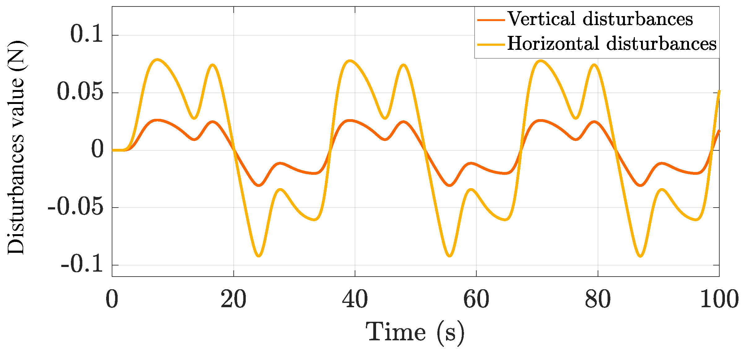
4. Simulation Results and Discussion

In this section, we present the results of our simulations carried out on the TRMS model to assess the efficiency of our proposed controller. The simulations were conducted using the TRMS template in the MATLAB/Simulink environment.

In all the simulation results, the initial conditions are chosen as

$${[x_{1,i}\left(0\right),x_{2,i}\left(0\right),x_{3,i}\left(0\right)]}^T={[0,0,0]}^T$$

The design parameters are chosen as follows: $p=107/100,a_{1,i}=a_{2,i}=0.1,{\gamma }_{1,i}=1,{\beta }_{1,i}=1,$ and ${\gamma }_{2,i}={\gamma }_{3,i}=4/3$. Additionally, the NN estimators ${\mathcal{W}}_{1,i}^T{\mathsf{\Phi }}_{1,i}$ and ${\mathcal{W}}_{2,i}^T{\mathsf{\Phi }}_{2,i}$ both include six nodes [43]. The RBFNN used in this study is a standard three-layer architecture, consisting of an input layer, a hidden layer, and an output layer. The hidden layer contains six neurons, corresponding to the six nodes mentioned earlier, with each neuron utilizing a Gaussian activation function. The width of the RBFNN is set to four. The centers of the Gaussian functions are defined as follows: ${\mu }_{1,i}=\left[\begin{array}{ccccc}-2\hfill & -1\hfill & 0\hfill & 1\hfill & 2\hfill \\ -2\hfill & -1\hfill & 0\hfill & 1\hfill & 2\hfill \\ -2\hfill & -1\hfill & 0\hfill & 1\hfill & 2\hfill \\ -2\hfill & -1\hfill & 0\hfill & 1\hfill & 2\hfill \\ -3\hfill & -1\hfill & 0\hfill & 1\hfill & 3\hfill \\ -3\hfill & -1\hfill & 0\hfill & 1\hfill & 3\hfill \end{array}\right]$, ${\mu }_{2,i}=\left[\begin{array}{cccccccc}-3\hfill & -2\hfill & -1\hfill & 0\hfill & 0\hfill & 1\hfill & 2\hfill & 3\hfill \\ -3\hfill & -2\hfill & -1\hfill & 0\hfill & 0\hfill & 1\hfill & 2\hfill & 3\hfill \\ -3\hfill & -2\hfill & -1\hfill & 0\hfill & 0\hfill & 1\hfill & 2\hfill & 3\hfill \\ -3\hfill & -2\hfill & -1\hfill & 0\hfill & 0\hfill & 1\hfill & 2\hfill & 3\hfill \\ -2\hfill & -2\hfill & -1\hfill & 0\hfill & 0\hfill & 1\hfill & 2\hfill & 3\hfill \\ -2\hfill & -2\hfill & -1\hfill & 0\hfill & 0\hfill & 1\hfill & 2\hfill & 3\hfill \end{array}\right]$.

Several scenarios were created to examine the robustness of the TRMS. These scenarios included normal operation with external disturbances and the presence of various sensor faults. We started by testing the fixed-time adaptive neural controller (FxTANC) without any faults and without the adaptive fault estimation scheme. Next, we tested the proposed fault-tolerant fixed-time adaptive neural controller (FTFxTANC), which incorporates the adaptive fault estimation scheme to handle sensor faults for angular velocities, including multiplicative faults (loss of effectiveness) and additive faults (bias, drift, loss of accuracy). To guarantee a bounded and smoother profile, the desired trajectory was subjected to a filtering process.

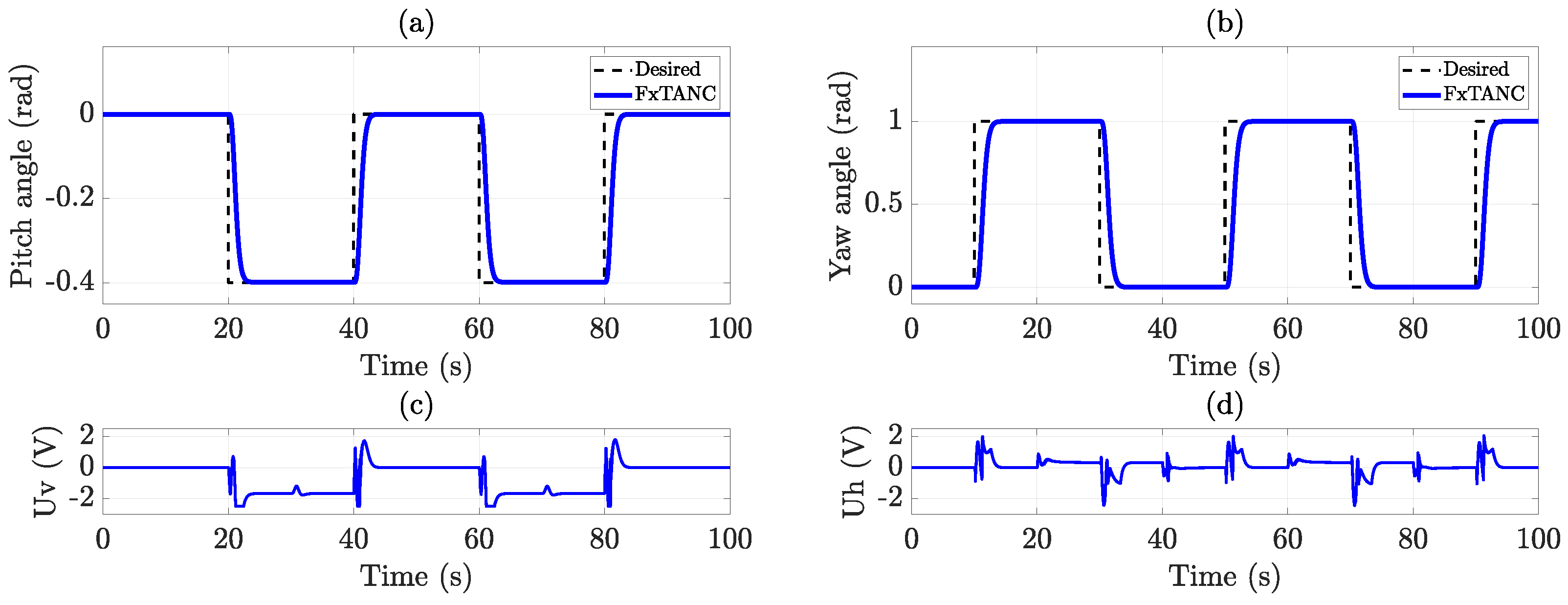
4.1. Case 1: Square-Wave Tracking

In the first test, our focus was on evaluating the performance of the TRMS when subjected to square-wave reference signals for both the vertical and horizontal subsystems. Figure 4 shows the test results, highlighting the regulation behaviors demonstrated by the developed FxTANC. Figure 4a,b illustrate that the pitch and yaw angle responses closely followed the desired square-wave trajectory, showcasing the controller’s ability to handle the cross-coupling complexities between the vertical and horizontal subsystems of the TRMS. This indicates robust performance in the presence of abrupt changes in the reference signal. Moreover, the control inputs in Figure 4c,d remained within the constrained range of [−2.5 V, 2.5 V] [22], showcasing the controller’s ability to maintain system stability without exceeding the actuator limits, which is crucial for practical applications.

Table 1. Control gains.

Subsystem	Gains
Vertical	$k_{1,v}=13.9650$
	$k_{2,v}=47.3081$
	$k_{3,v}=15.5180$
Horizontal	$k_{1,h}=21.0615$
	$k_{2,h}=50.0000$
	$k_{3,h}=29.5547$

presents the optimal parameters of $k_{1,i},k_{2,i}$, and $k_{3,i}$ used in all the scenarios.

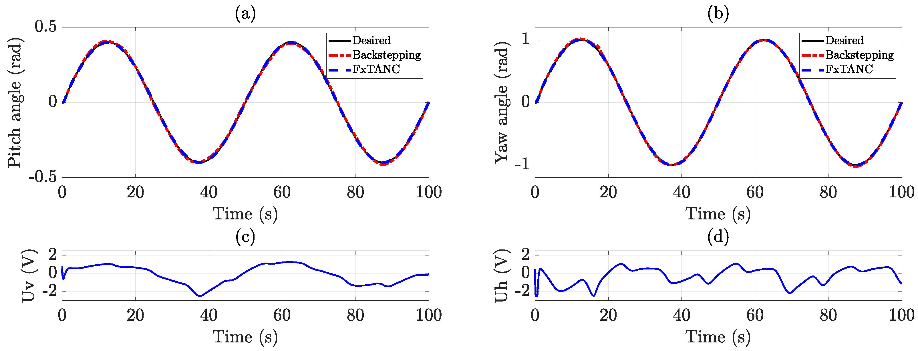
4.2. Case 2: Sine-Wave Tracking

The second scenario involved tracking sinusoidal reference signals, which were given by the following two equations: $y_{d,v}\left(t\right)=0.4sin\left(0.02t\right)$ and $y_{d,h}\left(t\right)=sin\left(0.02t\right)$. Note that the complexity of this test was increased by the introduction of external disturbances, as depicted in Figure 5. The results in Figure 6 demonstrate the tracking capabilities and robustness of the proposed FxTANC. Figure 6a,b show a comparison of the results with the nominal backstepping controller in [44]. The FxTANC exhibited superior tracking performance, maintaining closer adherence to the desired trajectory, despite disturbances. The voltages delivered to the main and tail rotors, as displayed in Figure 6c,d, reveal that the values were maintained within a restricted acceptable range.

4.3. Case 3: Bias Sensor Faults

In this test, we introduced a bias fault into the sensor readings to evaluate the system’s performance under such conditions. Figure 7 illustrates the robustness of the FTFxTANC, which managed the bias fault introduced into the velocity sensor. To simulate this fault scenario, a bias was introduced into the sensors at time $t_f=20$ s, with bias values of $f_{a,v}$ = 0.4 rad/s and $f_{a,h}$ = 0.8 rad/s. The simulation results presented in Figure 7a,b demonstrate the robust nature of the proposed controller, which effectively decreased the impact of the bias fault, ensuring stability and accurate tracking. The fault estimation, as shown in Figure 7c,d, effectively identified and compensated for sensor biases, showcasing the controller’s robustness and adaptability to these biases. Furthermore, Figure 7e,f depict the input voltages of the two DC motors of the TRMS provided by the proposed controller.

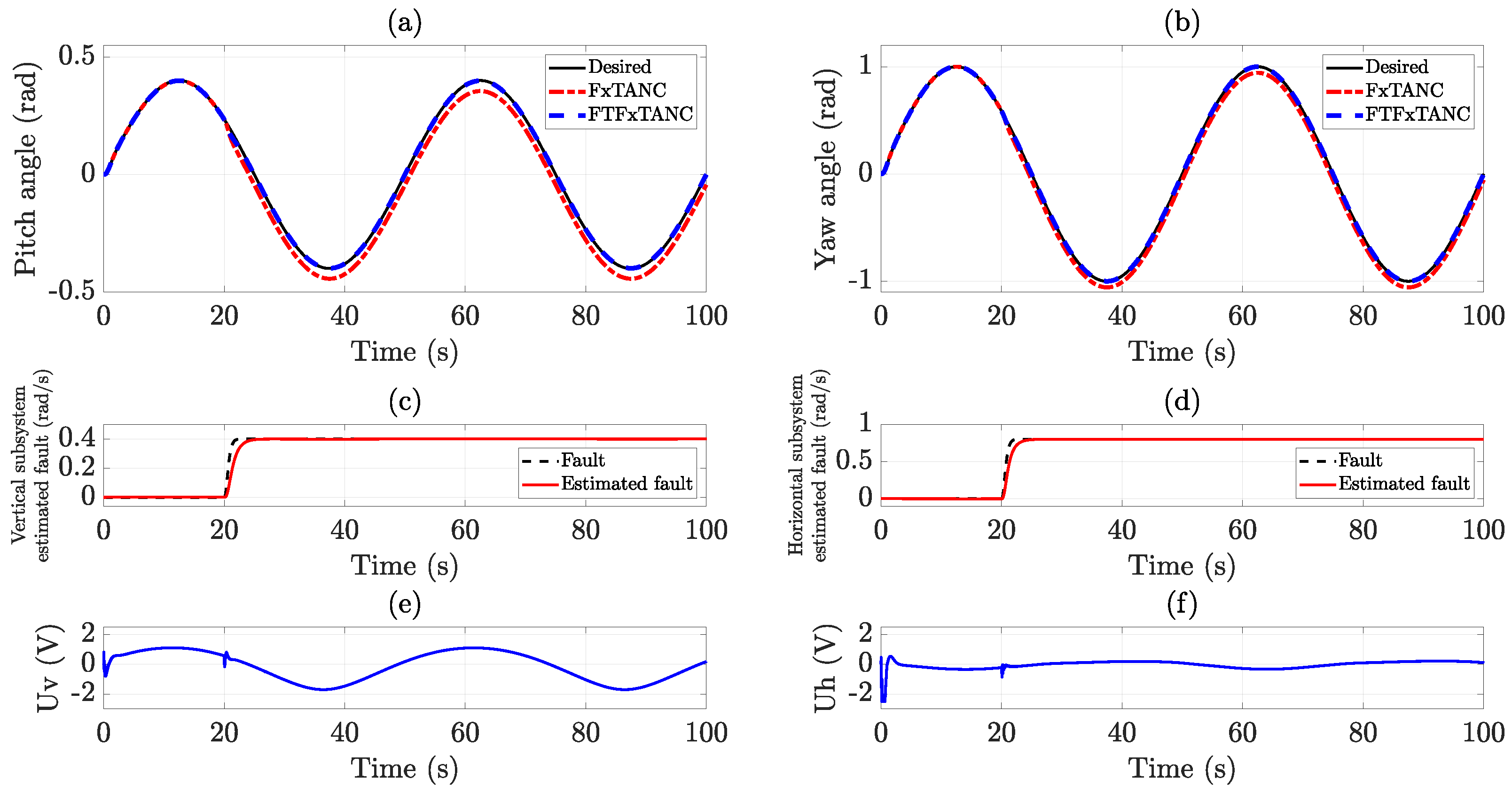
4.4. Case 4: Drift Sensor Faults

In this test, we focused on assessing the TRMS in the context of a drift fault affecting the velocity sensor. We introduced a fault into the sensors at time $t_f=20$ s, with drift coefficients of $f_{a,v}=0.01$ and $f_{a,h}=0.02$, knowing that even small deviations in sensor readings over time can potentially affect control accuracy. The results depicted in Figure 8 reveal how well the FTFxTANC handled this kind of fault. In Figure 8a,b, it can be seen that the proposed FTFxTANC effectively managed the drift fault, keeping the helicopter on track despite the drifting sensor readings. Figure 8c,d present the fault and its estimation, illustrating the adaptive fault estimator’s proficiency in tracking and compensating for drift faults. Figure 8e,f provide a closer look at the control signals that guide the helicopter, which remained within safe limits.

4.5. Case 5: Loss of Accuracy Sensor Faults

In this test, we focused on addressing the issue of accuracy loss in the TRMS’s velocity sensor. When this situation occurs, the sensor can become less accurate, providing incorrect readings that may confuse the control system and affect the helicopter’s performance. To evaluate how effectively the controller handled this problem, we made the sensor less accurate at time $t_f=20$ s. As seen in Figure 9, we introduced this accuracy loss defect with $f_{a,v}=0.15$ rad/s and $f_{a,h}=0.4$ rad/s. In Figure 9a,b, it is clear that the proposed FTFxTANC is capable of handling this kind of fault. Despite the inaccurate sensor readings, the controller kept the helicopter on track, while the fault estimation, as shown in Figure 9c,d, accurately identified and compensated for the sensor biases. The input voltages of the TRMS fell within an admissible range, as depicted in Figure 9e,f.

4.6. Case 6: Loss of Effectiveness Sensor Faults

The final case of our investigation focused on the tolerance of the controller against sensor faults, specifically the velocity sensor. When this situation occurs, the sensor becomes much less reliable, providing readings that are only accurate within a small percentage. We simulated the loss of effectiveness at time $t_f=20$ s to test the controller’s ability to handle this kind of failure. Figure 10 illustrates a 55% reduction in the velocity sensor’s effectiveness. The angle responses, as shown in Figure 10a,b, demonstrate that the proposed FTFxTANC effectively managed the reduced sensor effectiveness, maintaining close adherence to the desired trajectory. However, this kind of fault led to instability and performance degradation with the FxTANC. The fault estimation, as shown in Figure 10c,d, successfully detected and compensated for the loss of effectiveness, highlighting the robustness of the control scheme. Figure 10e,f depict the control voltages of the FTFxTANC, which exhibited similar observations and remained within admissible values.

5. Conclusions

In this paper, we introduced a fault-tolerant fixed-time adaptive neural control scheme for the challenging Twin-Rotor MIMO System, specifically addressing sensor faults. The proposed scheme integrates the backstepping technique, an RBFNN, and an adaptive fault estimator. This combination ensures system stability, robustness against sensor faults, and fixed-time convergence, as validated by Lyapunov-based stability analysis. The simulation results demonstrate the potential and effectiveness of our proposed approach in practical control applications. Future research should focus on experimental validation, addressing actuator faults, and exploring hybrid control strategies to further enhance the robustness and applicability of the control framework.

References

1. Abdelmaksoud, S.I.; Mailah, M.; Abdallah, A.M. Control strategies and novel techniques for autonomous rotorcraft unmanned aerial vehicles: A review. IEEE Access 2020, 8, 195142–195169. [Google Scholar] [CrossRef]
2. Zhang, Y.; Jiang, J. Bibliographical review on reconfigurable fault-tolerant control systems. Annu. Rev. Control 2008, 32, 229–252. [Google Scholar] [CrossRef]
3. Han, J.; Zhang, J.; Lv, C.; He, C.; Wei, H.; Zhao, S. Robust Fault Tolerant Path Tracking Control for Intelligent Vehicle under Steering System Faults. IEEE Trans. Intell. Veh. 2024. early access. [Google Scholar] [CrossRef]
4. Glida, H.-E.; Sentouh, C.; Chelihi, A.; Floris, J.; Popieul, J.-C. Event-Triggered Adaptive Fault-Tolerant Control Based on Sliding Mode/Neural Network for Lane Keeping Assistance Systems in Steer-by-Wire Vehicles. IEEE Trans. Intell. Veh. 2024. early access. [Google Scholar] [CrossRef]
5. Lippiello, V.; Ruggiero, F.; Serra, D. Emergency landing for a quadrotor in case of a propeller failure: A backstepping approach. In Proceedings of the 2014 IEEE/RSJ International Conference on Intelligent Robots and Systems, Chicago, IL, USA, 14–18 September 2014; IEEE: Piscataway, NJ, USA, 2014; pp. 4782–4788. [Google Scholar]
6. Nasiri, A.; Nguang, S.K.; Swain, A.; Almakhles, D. Passive actuator fault tolerant control for a class of MIMO nonlinear systems with uncertainties. Int. J. Control 2019, 92, 693–704. [Google Scholar] [CrossRef]
7. Raval, S.; Patel, H.R.; Patel, S.; Shah, V.A. Passive fault-tolerant control scheme for nonlinear level control system with parameter uncertainty and actuator fault. In Proceedings of the North American Fuzzy Information Processing Society Annual Conference, Halifax, NS, Canada, 31 May–3 June 2022; Springer: Cham, Switzerland, 2022; pp. 229–242. [Google Scholar]
8. Su, Y.; Yu, P.; Gerber, M.J.; Ruan, L.; Tsao, T.C. Fault-tolerant control of an overactuated uav platform built on quadcopters and passive hinges. IEEE/ASME Trans. Mechatron. 2023, 29, 602–613. [Google Scholar] [CrossRef]
9. Ke, C.; Cai, K.Y.; Quan, Q. Uniform passive fault-tolerant control of a quadcopter with one, two, or three rotor failure. IEEE Trans. Robot. 2023, 39, 4297–4311. [Google Scholar] [CrossRef]
10. Yao, Z.; Kan, Z.; Zhen, C.; Shao, H.; Li, D. Fault-Tolerant control for carrier-based UAV based on sliding mode method. Drones 2023, 7, 194. [Google Scholar] [CrossRef]
11. Wang, B.; Shen, Y.; Li, N.; Zhang, Y.; Gao, Z. An adaptive sliding mode fault-tolerant control of a quadrotor unmanned aerial vehicle with actuator faults and model uncertainties. Int. J. Robust Nonlinear Control 2023, 33, 10182–10198. [Google Scholar] [CrossRef]
12. Zeghlache, S.; Rahali, H.; Djerioui, A.; Benyettou, L.; Benkhoris, M.F. Robust adaptive backstepping neural networks fault tolerant control for mobile manipulator UAV with multiple uncertainties. Math. Comput. Simul. 2024, 218, 556–585. [Google Scholar] [CrossRef]
13. Bounemeur, A.; Chemachema, M.; Essounbouli, N. Indirect adaptive fuzzy fault-tolerant tracking control for MIMO nonlinear systems with actuator and sensor failures. ISA Trans. 2018, 79, 45–61. [Google Scholar] [CrossRef]
14. Ahmadi, K.; Asadi, D.; Merheb, A.; Nabavi-Chashmi, S.Y.; Tutsoy, O. Active fault-tolerant control of quadrotor UAVs with nonlinear observer-based sliding mode control validated through hardware in the loop experiments. Control Eng. Pract. 2023, 137, 105557. [Google Scholar] [CrossRef]
15. Shabbir, W.; Aijun, L.; Yuwei, C. Neural network-based sensor fault estimation and active fault-tolerant control for uncertain nonlinear systems. J. Frankl. Inst. 2023, 360, 2678–2701. [Google Scholar] [CrossRef]
16. Nguyen, N.P.; Pitakwatchara, P. Attitude fault-tolerant control of aerial robots with sensor faults and disturbances. Drones 2023, 7, 156. [Google Scholar] [CrossRef]
17. Hu, X.; Wang, B.; Shen, Y.; Fu, Y.; Li, N. Disturbance observer-enhanced adaptive fault-tolerant control of a quadrotor UAV against actuator faults and disturbances. Drones 2023, 7, 541. [Google Scholar] [CrossRef]
18. Fliess, M.; Join, C. Model-free control. Int. J. Control 2013, 86, 2228–2252. [Google Scholar] [CrossRef]
19. Glida, H.E.; Chelihi, A.; Abdou, L.; Sentouh, C.; Perozzi, G. Trajectory tracking control of a coaxial rotor drone: Time-delay estimation-based optimal model-free fuzzy logic approach. ISA Trans. 2023, 137, 236–247. [Google Scholar] [CrossRef] [PubMed]
20. Glida, H.E.; Sentouh, C.; Rath, J.J. Optimal Model-Free Finite-Time Control Based on Terminal Sliding Mode for a Coaxial Rotor. Drones 2023, 7, 706. [Google Scholar] [CrossRef]
21. Glida, H.E.; Abdou, L.; Chelihi, A.; Sentouh, C.; Hasseni, S.E.I. Optimal model-free backstepping control for a quadrotor helicopter. Nonlinear Dyn. 2020, 100, 3449–3468. [Google Scholar] [CrossRef]
22. Feedback Instruments Ltd. Twin Rotor MIMO System Control Experiments 33-949S; Feedback Instruments Ltd.: Crowborough, UK, 2006. [Google Scholar]
23. Faris, H.; Aljarah, I.; Al-Betar, M.A.; Mirjalili, S. Grey wolf optimizer: A review of recent variants and applications. Neural Comput. Appl. 2018, 30, 413–435. [Google Scholar] [CrossRef]
24. Hatta, N.; Zain, A.M.; Sallehuddin, R.; Shayfull, Z.; Yusoff, Y. Recent studies on optimisation method of Grey Wolf Optimiser (GWO): A review (2014–2017). Artif. Intell. Rev. 2019, 52, 2651–2683. [Google Scholar] [CrossRef]
25. Lai, W.; Kuang, M.; Wang, X.; Ghafariasl, P.; Sabzalian, M.H.; Lee, S. Skin cancer diagnosis (SCD) using Artificial Neural Network (ANN) and Improved Gray Wolf Optimization (IGWO). Sci. Rep. 2023, 13, 19377. [Google Scholar] [CrossRef]
26. Cai, Z.; Dai, S.; Ding, Q.; Zhang, J.; Xu, D.; Li, Y. Gray wolf optimization-based wind power load mid-long term forecasting algorithm. Comput. Electr. Eng. 2023, 109, 108769. [Google Scholar] [CrossRef]
27. Perozzi, G.; Efimov, D.; Biannic, J.M.; Planckaert, L. Trajectory tracking for a quadrotor under wind perturbations: Sliding mode control with state-dependent gains. J. Frankl. Inst. 2018, 355, 4809–4838. [Google Scholar] [CrossRef]
28. Kapnopoulos, A.; Kazakidis, C.; Alexandridis, A. Quadrotor trajectory tracking based on backstepping control and radial basis function neural networks. Results Control Optim. 2024, 14, 100335. [Google Scholar] [CrossRef]
29. Younes, Y.A.; Drak, A.; Noura, H.; Rabhi, A.; Hajjaji, A.E. Robust model-free control applied to a quadrotor UAV. J. Intell. Robot. Syst. 2016, 84, 37–52. [Google Scholar] [CrossRef]
30. Barth, J.M.; Condomines, J.P.; Bronz, M.; Moschetta, J.M.; Join, C.; Fliess, M. Model-free control algorithms for micro air vehicles with transitioning flight capabilities. Int. J. Micro Air Veh. 2020, 12, 1756829320914264. [Google Scholar] [CrossRef]
31. Guettal, L.; Glida, H.E.; Chelihi, A. Adaptive fuzzy-neural network based decentralized backstepping controller for attitude control of quadrotor helicopter. In Proceedings of the 2020 1st International Conference on Communications, Control Systems and Signal Processing (CCSSP), El Oued, Algeria, 16–17 May 2020; IEEE: Piscataway, NJ, USA, 2020; pp. 394–399. [Google Scholar]
32. Bey, O.; Chemachema, M. Finite-time event-triggered output-feedback adaptive decentralized echo-state network fault-tolerant control for interconnected pure-feedback nonlinear systems with input saturation and external disturbances: A fuzzy control-error approach. Inf. Sci. 2024, 669, 120557. [Google Scholar] [CrossRef]
33. Hernández-González, O.; Ramírez-Rasgado, F.; Farza, M.; Guerrero-Sánchez, M.E.; Astorga-Zaragoza, C.M.; M’Saad, M.; Valencia-Palomo, G. Observer for Nonlinear Systems with Time-Varying Delays: Application to a Two-Degrees-of-Freedom Helicopter. Aerospace 2024, 11, 206. [Google Scholar] [CrossRef]
34. Zuo, Z.; Tian, B.; Defoort, M.; Ding, Z. Fixed-Time Consensus Tracking for Multiagent Systems With High-Order Integrator Dynamics. IEEE Trans. Autom. Control 2018, 63, 563–570. [Google Scholar] [CrossRef]
35. Ba, D.; Li, Y.X.; Tong, S. Fixed-time adaptive neural tracking control for a class of uncertain nonstrict nonlinear systems. Neurocomputing 2019, 363, 273–280. [Google Scholar] [CrossRef]
36. Du, H.; Shao, H.; Yao, P. Adaptive neural network control for a class of low-triangular-structured nonlinear systems. IEEE Trans. Neural Netw. 2006, 17, 509–514. [Google Scholar] [CrossRef] [PubMed]
37. Ge, S.S.; Hang, C.C.; Lee, T.H.; Zhang, T. Stable Adaptive Neural Network Control; Springer Science & Business Media: Berlin/Heidelberg, Germany, 2013; Volume 13. [Google Scholar]
38. Shaik, F.A.; Purwar, S. A nonlinear state observer design for 2-DOF twin rotor system using neural networks. In Proceedings of the 2009 International Conference on Advances in Computing, Control, and Telecommunication Technologies, Bangalore, India, 28–29 December 2009; IEEE: Piscataway, NJ, USA, 2009; pp. 15–19. [Google Scholar] [CrossRef]
39. Glida, H.E.; Abdou, L.; Chelihi, A.; Sentouh, C.; Perozzi, G. Optimal model-free fuzzy logic control for autonomous unmanned aerial vehicle. Proc. Inst. Mech. Eng. Part G J. Aerosp. Eng. 2022, 236, 952–967. [Google Scholar] [CrossRef]
40. Mirjalili, S.; Mirjalili, S.M.; Lewis, A. Grey wolf optimizer. Adv. Eng. Softw. 2014, 69, 46–61. [Google Scholar] [CrossRef]
41. Hao, P.; Sobhani, B. Application of the improved chaotic grey wolf optimization algorithm as a novel and efficient method for parameter estimation of solid oxide fuel cells model. Int. J. Hydrogen Energy 2021, 46, 36454–36465. [Google Scholar] [CrossRef]
42. Li, H.; Liu, X.; Huang, Z.; Zeng, C.; Zou, P.; Chu, Z.; Yi, J. Newly emerging nature-inspired optimization-algorithm review, unified framework, evaluation, and behavioural parameter optimization. IEEE Access 2020, 8, 72620–72649. [Google Scholar] [CrossRef]
43. He, C.; Wu, J.; Dai, J.; Zhe, Z.; Tong, T. Fixed-Time Adaptive Neural Tracking Control for a Class of Uncertain Nonlinear Pure-Feedback Systems. IEEE Access 2020, 8, 28867–28879. [Google Scholar] [CrossRef]
44. Haruna, A.; Mohamed, Z.; Efe, M.Ö.; Basri, M.A.M. Dual boundary conditional integral backstepping control of a twin rotor MIMO system. J. Frankl. Inst. 2017, 354, 6831–6854. [Google Scholar] [CrossRef]
Figure 1. Stability comparison for different initial conditions.
Drones 08 00467 g001
Figure 2. Twin-Rotor MIMO System.
Drones 08 00467 g002
Figure 3. Fixed-time fault-tolerant adaptive neural control structure for the TRMS helicopter.
Drones 08 00467 g003
Figure 4. Tracking performance for square-wave reference signals: (a,b) attitude angles, (c,d) input voltages.
Drones 08 00467 g004
Figure 5. External disturbances.
Drones 08 00467 g005
Figure 6. Tracking performance for sine-wave reference signals with disturbances: (a,b) attitude angles, (c,d) input voltages.
Drones 08 00467 g006
Figure 7. Tracking performance for sine-wave reference signals with a bias fault: (a,b) attitude angles, (c,d) bias fault estimates, (e,f) input voltages.
Drones 08 00467 g007
Figure 8. Tracking performance for sine-wave reference signals with drift fault: (a,b) attitude angles, (c,d) drift fault estimates, (e,f) input voltages.
Drones 08 00467 g008
Figure 9. Tracking performance for sine-wave reference signals with loss of accuracy fault: (a,b) attitude angles, (c,d) loss of accuracy fault estimates, (e,f) input voltages.
Drones 08 00467 g009
Figure 10. Tracking performance for sine-wave reference signals with loss of effectiveness fault: (a,b) attitude angles, (c,d) loss of effectiveness fault estimates, (e,f) input voltages.
Drones 08 00467 g010