Abstract
This study deals with the path-following guidance of a fixed-wing unmanned aerial system (UAS) in conjunction with parameter adaptation. Utilizing a backstepping control design approach, a path-following control algorithm is formulated for the roll command, accounting for the approximated closed-loop roll control. The inaccurate time constant is estimated by employing a parameter adaptation algorithm. The proposed guidance algorithm is first validated via the hardware-in-the-loop simulation environment, followed by flight tests on an actual UAV platform to demonstrate that both tracking performance and control robustness are improved over various shape of reference paths.
1. Introduction
Unmanned aerial systems (UASs) have been suggested as substitutes for piloted aircraft in various missions. When a UAS vehicle is operated in an unknown environment, the autonomous operation of the UAS with minimal human intervention is an essential prerequisite to achieve the mission objectives. That is, given a mission objective, the UAS should be operated seamlessly from mission planning down to the low-level control function. The path-planning algorithm at the top level computes a discrete path skeleton of the best route, and then a smooth path curve is obtained by using a path generation scheme. The generated path curve should be dynamically feasible, that is, it should be a flyable path that satisfies the dynamic constraints of the UAS. Finally, a guidance controller is used to guide the UAS to the designated path.
The guidance problem of the UAS is solved in two distinct steps; trajectory tracking [1,2] and path following [3,4]. While the trajectory tracking of the UAS implies following a time-parameterized reference path, the path following is only required to follow a path without any temporal parameterization. The basic requirement of the path-following control law is, with controlled forward ground speed, to provide the actions by which the UAS is driven to the path. In the trajectory-tracking problem, it is common to have direct control on the along-track direction to ensure accurate tracking; however, it has been reported that better convergence to a path is achieved by indirect control with a virtual target that moves accordingly [5].
In general, the path-following problem is simpler than the trajectory-tracking problem and is often applied in cases where the accuracy of path following is more critical than the temporal exactness. For this purpose, the path-following problem has been addressed by using various control approaches in the literature. In the ocean community, 3D path following is proposed in ref. [6] to control marine vehicles, where the curvature and torsion characteristics of the 3D desired path is considered to guarantee fast convergence of error. Zhang [7] proposed a path-following control for under-actuated marine vehicles. In this paper, the path-following guidance employs the line of sight (LOS) method to manage underactuated motion dynamics, while integrating the sliding mode control, which is recognized for its robustness against external disturbances. Miao [8] proposed a robust path-following control for underactuated autonomous underwater vehicle via a backstepping scheme integrated with extended state observers. For UAS applications, a precise path-tracking control law is proposed in ref. [9], where global stability can be achieved by combining a flatness-based control and a guidance law based on nonlinear dynamic inversion. Park et al. [10] proposed a nonlinear guidance control law which is simple and straightforward, in conjunction with the experimental validation from flight tests. A constrained trajectory-tracking problem was addressed in ref. [11]. In this paper, taking into account the velocity constraints between two positive constants, the control Lyapunov function (CLF) is utilized to construct the set of all constrained inputs that are feasible with respect to the CLF. The actual control input is then selected from this feasible set to implicitly account for the velocity constraints. Meanwhile, vector field-based techniques are widely employed to guide the UAS to the given path curve [12,13,14,15,16]. The vector field provides smooth and stable path-following capabilities in complex environments with numerous obstacles while allowing easy implementation. In some studies, robust path-following control laws have been proposed against unknown disturbances, such as wind [13,17,18,19,20]. Various techniques, such as a disturbance interval observer [17] and RBF neural network [18,19], have been utilized to estimate and compensate for external disturbances within the model. In ref. [13], a curved path-following control law with increased robustness was proposed by adding an estimator for ground speed, which is difficult to measure directly. Kumar et al. [20] proposed a nonlinear guidance law inspired by pursuit guidance, which computes the airspeed and air-mass referenced angular speed command through the relative separation and look angle. In ref. [21], the UAV path-following law based on the global fast terminal sliding mode control method was derived by dividing it into an outer guidance loop and an inner control loop. Reinardt et al. [22] proposed an algorithm based on nonlinear model predictive control that directly generates actuator control commands.
Firstly, the UAV path-following model is divided into an outer guidance loop and an inner control loop. Then, the guidance loop and control loop controllers of the UAV are derived by a global fast terminal sliding mode control technique, which is able to guarantee the system state variables converge to expected values in finite time and eliminate the chattering phenomenon caused by the switching control action.
In this paper, the problem of path following of a UAS is addressed under the assumption of a unicycle kinematics model of the UAS. Similar to a two-step procedure presented in [5,23,24] for path following, a kinematic control law [25] is first considered to regulate the error with respect to the reference. Then, by taking into account the distinct mechanism for heading change of a fixed-wing UAS, a standard back-stepping scheme is incorporated to calculate the roll command that has an equivalent effect to the kinematic control law. The time constant of the approximated roll closed-loop is estimated on-line using a parameter adaptation scheme, yielding robust performance for actual implementation. In previous studies, the proposed algorithms have been validated solely through simulations; in contrast, the main contributions of this paper include:
- Derivation of a robust path-following guidance law, supported by theoretical proof and experimental validation.
- Low-level autopilot command generation incorporating the approximated roll closed-loop system where the modeling uncertainty is handled through parameter adaptation.
The proposed guidance algorithm is first analytically proven for its stability, and is then validated via a hardware-in-the-loop simulation (HILS) environment. Finally, several flight tests are conducted to demonstrate the feasibility of application on an actual UAS platform.
The paper is organized as follows: Section 2.1 describes the problem description of the guidance control for a UAS flying at a constant altitude. Section 2.2 is dedicated to the theoretical part of this paper, where a nonlinear adaptive guidance control law to follow a reference path generated by B-splines is explained in detail. The experimental results of extensive hardware-in-the-loop simulations are shown in Section 3.2, followed by the results of the flight tests in Section 3.3. Section 4 summarizes the concluding remarks.
2. Materials and Method
2.1. System Model
A fixed-wing UAS is assumed to fly at a constant altitude and speed. This is a reasonable assumption, since a low-level autopilot performs closed-loop control of airspeed and altitude. The inertial speed and the course of the UAS can be obtained directly from a GPS receiver. With this assumption, the motion can be described using simplified unicycle kinematics as follows:
where represents the inertial position of the UAS and is the course rate. When a fixed-wing UAS initiates a roll maneuver and turns without sideslip, the course rate is approximately calculated using the roll angle and the inertial speed as follows:
Since the autopilot of the UAS provides the feedback control of the roll, the closed-loop roll dynamics can be approximated by a first-order system:
where is the roll command and is the time constant of the closed-loop roll dynamics.
A fixed-wing UAS is assumed to fly along a path curve as illustrated in Figure 1. The reference path is assumed to be a smooth curve and is parametrized by the arc-length s from a starting point. Let be the position vector of the point on the path represented by the parameter s. A Serret–Frenet frame is attached at and is assumed to move along the curve. The x-axis of the S-F frame is aligned with the tangential direction at and has a reference bearing relative to the North direction N. The error vector is defined by , and can be decomposed into the along-track error and the cross-track error in the S-F frame. Then, the error kinematics of a fixed-wing UAS expressed in the S-F frame can be derived as follows [26]:
where the course error is defined by and represents the curvature at .
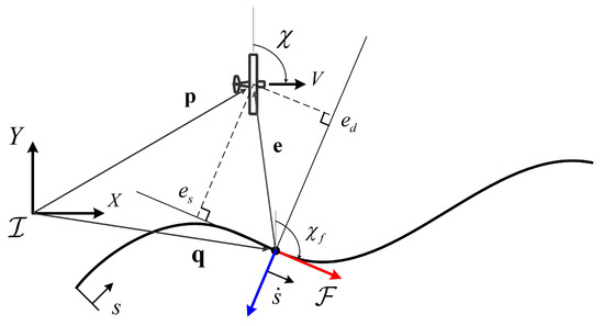
Figure 1.
Error coordinates definition with respect to the S-F frame ().
From Equation (4), the path-following problem simply becomes the problem of driving the error states , , and to zero with a given path. In other words, the moving S-F frame is treated as a virtual target, and the goal of path-following control is to guide the UAS to approach this virtual target. It is important to mention that the S-F frame moves along the path at a tangential velocity of . This tangential velocity of the virtual target provides an additional control action to effectively suppress the along-track error [27].
2.2. Nonlinear Guidance Control Law
In this section, the nonlinear adaptive path-following control law is presented. The objective of path-following control is to steer the UAS to the reference path despite an imperfect knowledge of system parameters. Here, given the kinematic control law for the course rate command and the arc-length rate command similar to that of ref. [27], a roll command is derived for a fixed-wing UAS which induces an equivalent control effort for the kinematic control law. In addition, the inaccurate system parameter is adaptively estimated for the use in the closed-loop control.
2.2.1. Kinematic Control Law
Let a bounded differentiable function be defined as,
where and [28]. This function is referred to as the approach angle because it provides an appropriate course angle of the UAS as dependent on the cross-track error , allowing the UAS to approach the path effectively. Once the UAS is on the path curve, the course angle is aligned with the tangential direction to the path, or the course error becomes zero.
Suppose that the reference path is parameterized by the arclength s, and for every s, the variables , , , and are properly defined. With the error system of the UAS described in Equation (4) and the approach angle defined in Equation (5), the following kinematic control law drives , , and asymptotically toward zero [26].
where the symbols , , and are positive gains, and denotes the derivative of the approach angle with respect to . The detailed stability proof of Equation (6) can be found in ref. [26]. Note that the term in Equation (6) forces the virtual target to move in a direction of reducing towards zero. Once the velocity command is determined in Equation (6b), a numerical integration scheme is utilized to propagate the position of the virtual target on the path.
2.2.2. Backstepping Design for Lateral Control
Suppose a fixed-wing aircraft is flying at a constant altitude, then the lateral control of the fixed-wing aircraft enables tracking the desired horizontal path. As described in Section 2.2.1, the heading control is performed using the course rate command to guide the aircraft to the desired path. However, considering the lateral coupling of fixed-wing aircraft, it is preferable to take advantage of the roll maneuver to induce the equivalent lateral control action instead of direct heading control. In this case, to compute the roll command, a straightforward approach is to compute the roll command directly from the course rate command using the relationship in Equation (2),
As described in Equation (3), the closed-loop roll dynamics can be approximated by a first-order system. This implies that the computed roll command may not be able to generate an immediate course rate due to the transient roll response, reducing the effectiveness of the control. Therefore, a roll command is computed to account for the roll dynamics, to make the course rate as .
To this end, following from a standard backstepping design method [29], an auxiliary control is introduced to define the roll dynamics as . Thus, the augmented system is given as follows,
where the auxiliary control is related to the roll command by
Given the desired course rate in Equation (6a), let be an error for the course rate. The time derivative of the course rate is given as,
Proposition 1.
Consider the error system of the UAS in Equation (8) and the approach angle δ defined in Equation (5). Assume that the speed of the UAS is non-zero and the reference path is given as a smooth curve. The variables of κ, , , and are properly defined in all s. Then, the auxiliary control,
where is a gain and is given in Equation (6a), asymptotically drives , , and towards zero, while .
Proof.
Let be a candidate Lyapunov function given by,
Differentiating with respect to time and rearranging using Equations (4) and (10) yields:
Substituting the from Equation (6a) and from Equation (6b), the expression reduces to
Selecting as the auxiliary control provided in Equation (11) results in,
In order to justify Equation (15), it should be noted that by the definition of in Equation (5), it is a monotonically decreasing odd function with respect to . Subsequently, the second term in Equation (15) becomes an even function with respect to and carries a negative sign. In particular, Equation (15) confirms that , , , and are bounded. Furthermore, is also bounded from Equation (5) as it is an alternative form of hyperbolic tangent, leading to asymptotes at .
One can readily show that is bounded because the first three terms are bounded by the above statement except the last terms. To show the boundedness of , the last term of Equation (6a) can be rearranged by the sum to product identity in trigonometry, as follows,
Note that the definition of the function, , is utilized to rearrange the term, and since the function is naturally bounded, it is straightforward to confirm the boundedness of . Because and are bounded, it follows that the auxiliary control in Equation (11) is properly defined with the limited roll angle such as .
To finalize the proof, observe that is both radially unbounded and non-increasing; thus, the set is a compact, positively invariant set. Let be the set of all points in where . After elaborating mathematically, it is readily identified that . From Equation (8), it is easy to verify that is an invariant set. By LaSalle’s invariance principle, it follows that every trajectory starting inside approaches as . In other words, since . Also, as . □
2.2.3. Adaptive Parameter Estimation
The roll closed-loop control system is a first-order system characterized by a time constant, as shown in Equation (3). Rearranging into an explicit form to obtain the roll command and substituting the auxiliary control in Equation (11) with , the bank angle command is obtained as follows:
In general, the time constant of roll control can be experimentally determined by the characteristics of the UAS airframe and the control gains of the autopilot, which implies that the value may be regarded to be uncertain within a certain bound. If the time constant has been experimentally estimated, denoted as , the actual roll command is likely computed by
where is an estimate of . Suppose is an approximated value and can vary depending on flight conditions, an algorithm that can adapt to parameter variations should be incorporated for the actual operation environment to estimate the accurate parameter. Defining the estimate error as , then the goal of the parameter adaptation technique is to make zero. For this purpose, let be a Lyapunov function candidate defined by
Differentiating with respect to time, one obtains
Similarly to the method used in the proof of Proposition 1, one substitutes the actual roll command using the auxiliary command in Equation (11) to obtain
Choosing as,
it follows that
Assuming that remains constant, the update rule for parameter adaptation can be directly derived from Equation (22), as shown below,
Proposition 2.
Let the control law in Equations (6) and (11). With the parameter update rule given by Equation (24), the roll command in Equation (18) ensures that the signals , , and asymptotically converge to zero, while .
Proof.
Equation (23) shows that is negative semi-definite. It is immediately evident that is bounded from below and is non-increasing, subsequently there exists a limit value of infinite time. Therefore, it is sufficient to show that is uniformly continuous. If this is the case, Barbalat’s lemma can be applied to guarantee . Now, it is immediately evident from Equation (23) that , , , , , and are all bounded. As in the proof of Proposition 1, it follows from Equation (6b) that is bounded, and from Equation (6a) that is also bounded. Using Equation (8), it is easy to see that are also bounded. Differentiating Equation (6a) with respect to time, one can show that all terms are bounded, including the last term, since the derivative of the sinc function is bounded [30] (see also Equation (16)). Hence, it can be inferred that is bounded. Furthermore, both and its time derivative are bounded. The time derivative of is computed as follows:
All terms on the right-hand side of Equation (25) are bounded, so that turns out to be bounded. Furthermore, is also bounded from Equation (24). Consider the second time derivative of as
where all terms on the right-hand side have been shown to be bounded. It follows that is bounded, and hence is uniformly continuous. Applying Barbalat’s lemma, it follows that as . □
3. Results
3.1. Performance Comparison via Numerical Simulation
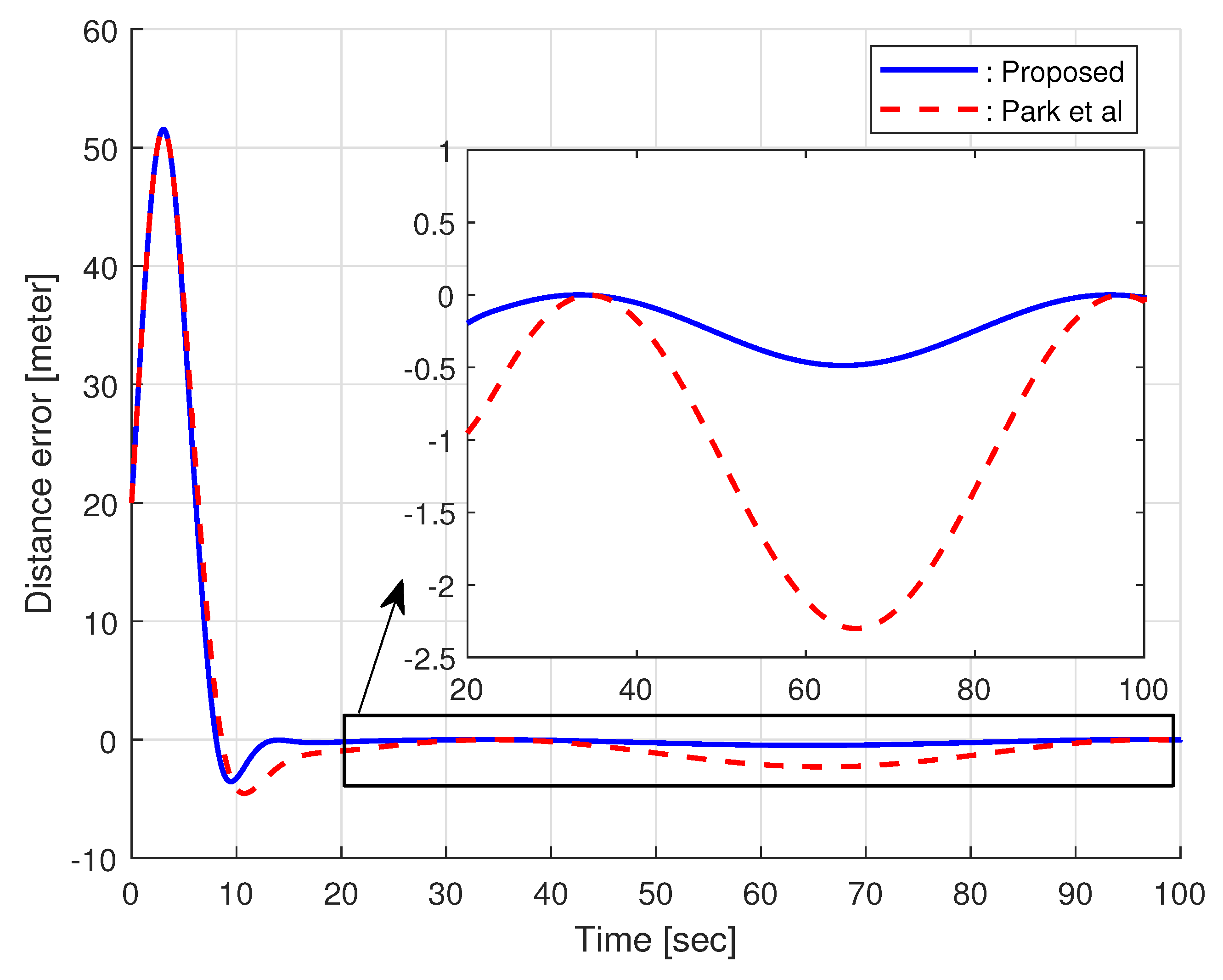
In order to evaluate the effectiveness of the proposed guidance law, a comparative study is carried out through numerical simulation. To this end, the nonlinear path-following guidance algorithm developed by Park et al. [10] was selected for comparison, which has been widely used in the open source community [31] due to its simple form and the effectiveness for fixed-wing guidance. The simplified kinematic models in Equations (1) and (2) are employed for the simulation. Meanwhile, the roll control system is approximated as a first-order system with proper PID gains, similar to previous discussion, and is excited by the non-zero disturbance as in Equation (27),
where the term on the right-hand side is considered as the disturbance excitation under the crosswind condition, which is deliberately included to evaluate the robustness of the guidance algorithms.
The reference path used for comparative simulations of each path guidance algorithm was chosen as a circular path, and the distance error from the circular path is defined as , where d is the radial distance of the UAV from the center of the circular path and is the reference radius. The comparison results are shown in Figure 2, with an enlarged view of the steady-state distance error after the initial transient. The solid line represents the distance error of the proposed guidance law, while the dashed line shows the distance error of the guidance algorithm of ref. [10].
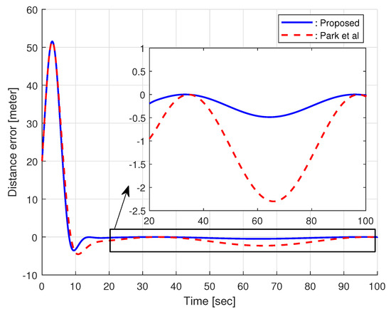
Figure 2.
Simulation result for comparative study: Distance error [10].
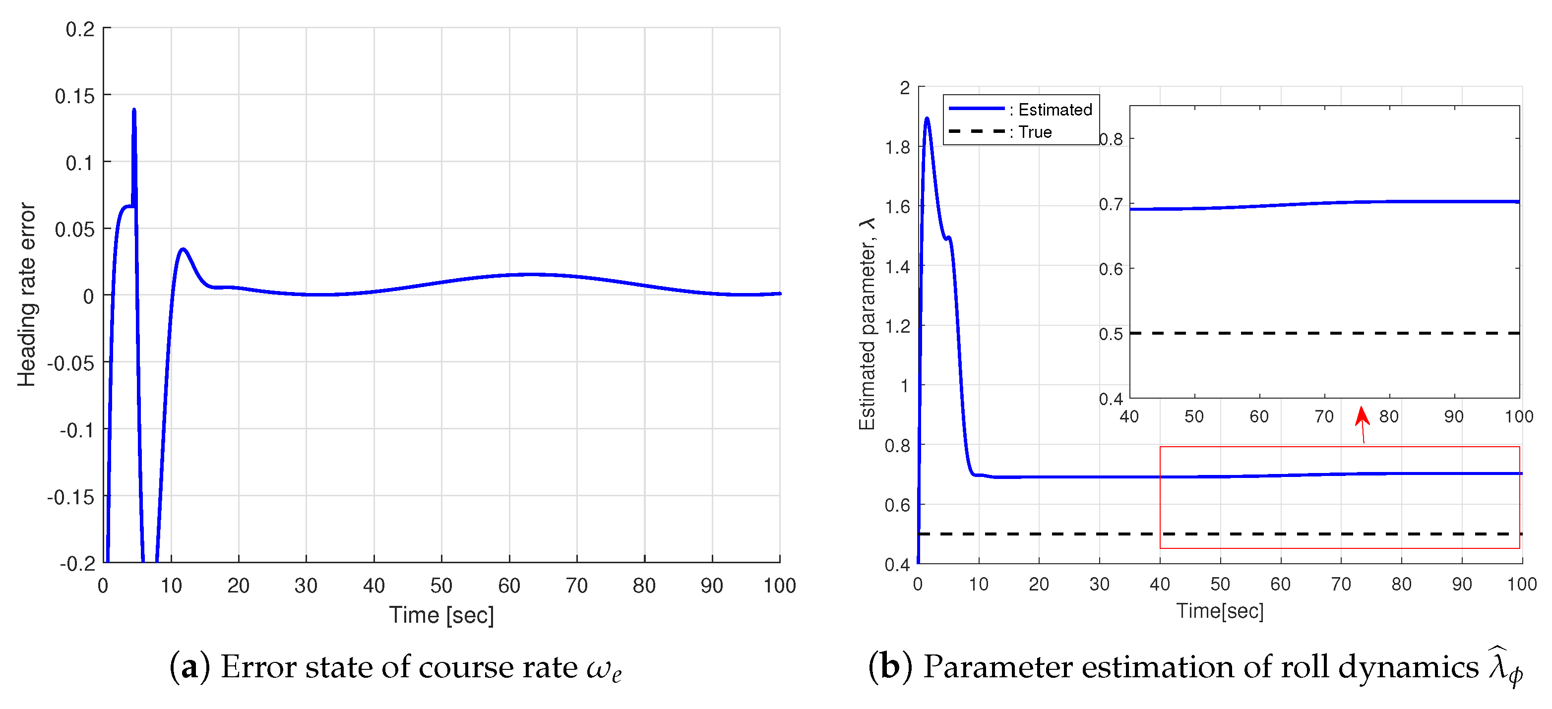
It should be noted that the constant wind disturbance in Equation (27) is assumed, leading to a periodic distance error with an offset from zero along the circular path. The steady error is attributed to the fact that the guidance law of ref. [10] has a form similar to proportional-derivative control, subsequently, the crosswind disturbance leads to the non-convergent distance error. This is also the case with the proposed algorithm. However, a key difference is that the proposed algorithm includes an input for the course rate in Equation (11). The course deviation from the reference due to the crosswind disturbance results in the non-zero course error rate , as depicted in Figure 3a, which enables mitigating the course angle errors when fed into the control input. Finally, the estimated time constant for closed-loop roll dynamics is shown in Figure 3b. The time constant effectively acts as the gain of the control action; as a result, it can help reduce the distance error slightly faster during the initial transient phase.
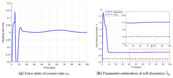
Figure 3.
Course rate error and the estimated time constant of the proposed guidance law.
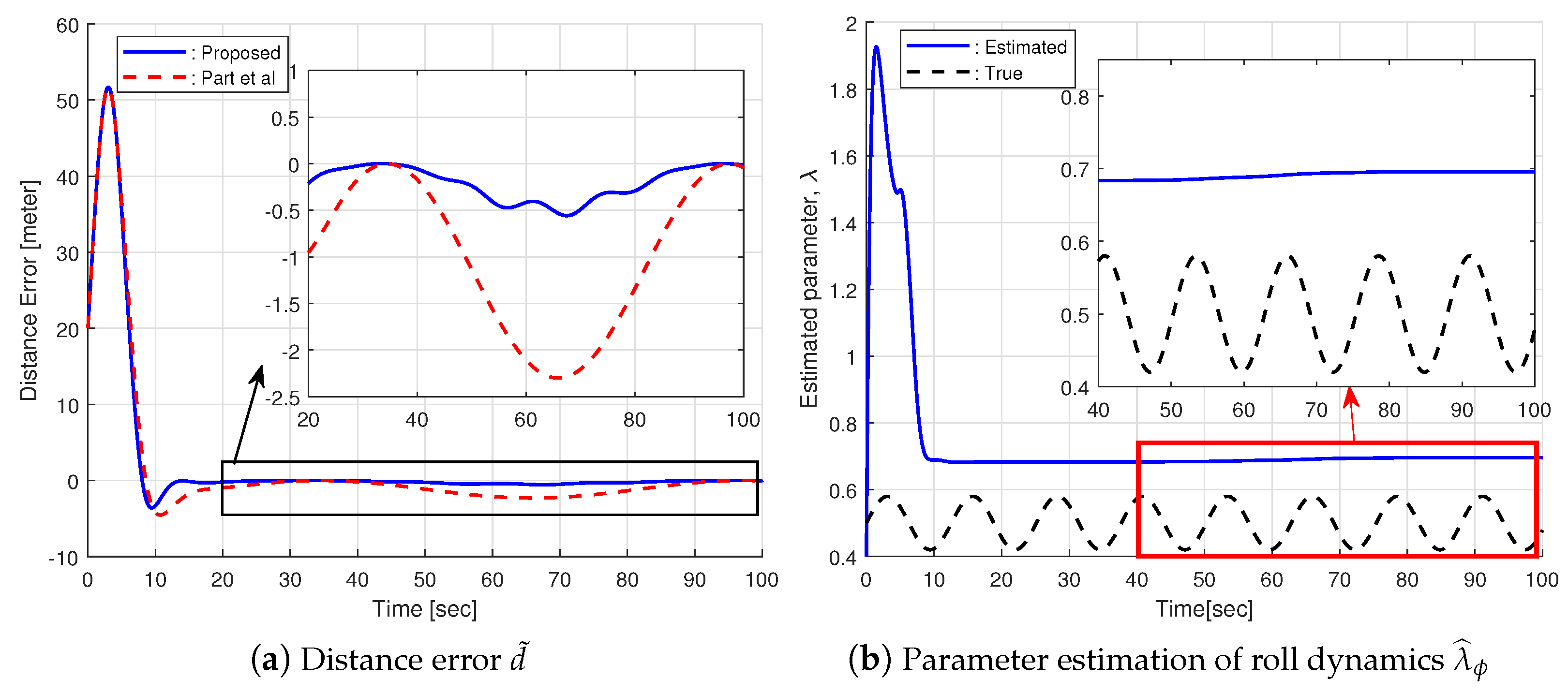
In addition, the issue of how the proposed algorithm performs if the time constant for closed-loop roll dynamics is time-varying in a complex manner is addressed. It is assumed that due to the instability of the low-level autopilot roll controller, the time constant in the actual closed-loop system is supposedly varying sinusoidally, as shown in Figure 4b. Since the time constant acts as the gain of the guidance control, as shown in Figure 4a in conjunction with Figure 2, it is observed that the sinusoidal time constant variation results in the complex variation of the distance error. Nonetheless, the estimated time constant for closed-loop roll dynamics appears to be unaffected, as one compares Figure 3b and Figure 4b. This is attributed to the fact that the excitation condition for parameter adaptation disappears with the error states convergence towards zero. For this reason, even when the parameter undergoes complex variations, the proposed algorithm demonstrates robustness to the unwanted parameter variations.
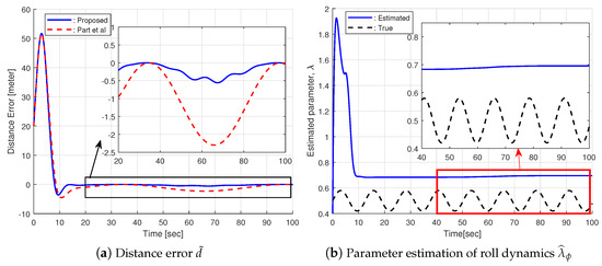
Figure 4.
Simulation results for time constant variations [10].
3.2. Performance Validation via HILS
3.2.1. HILS Environment
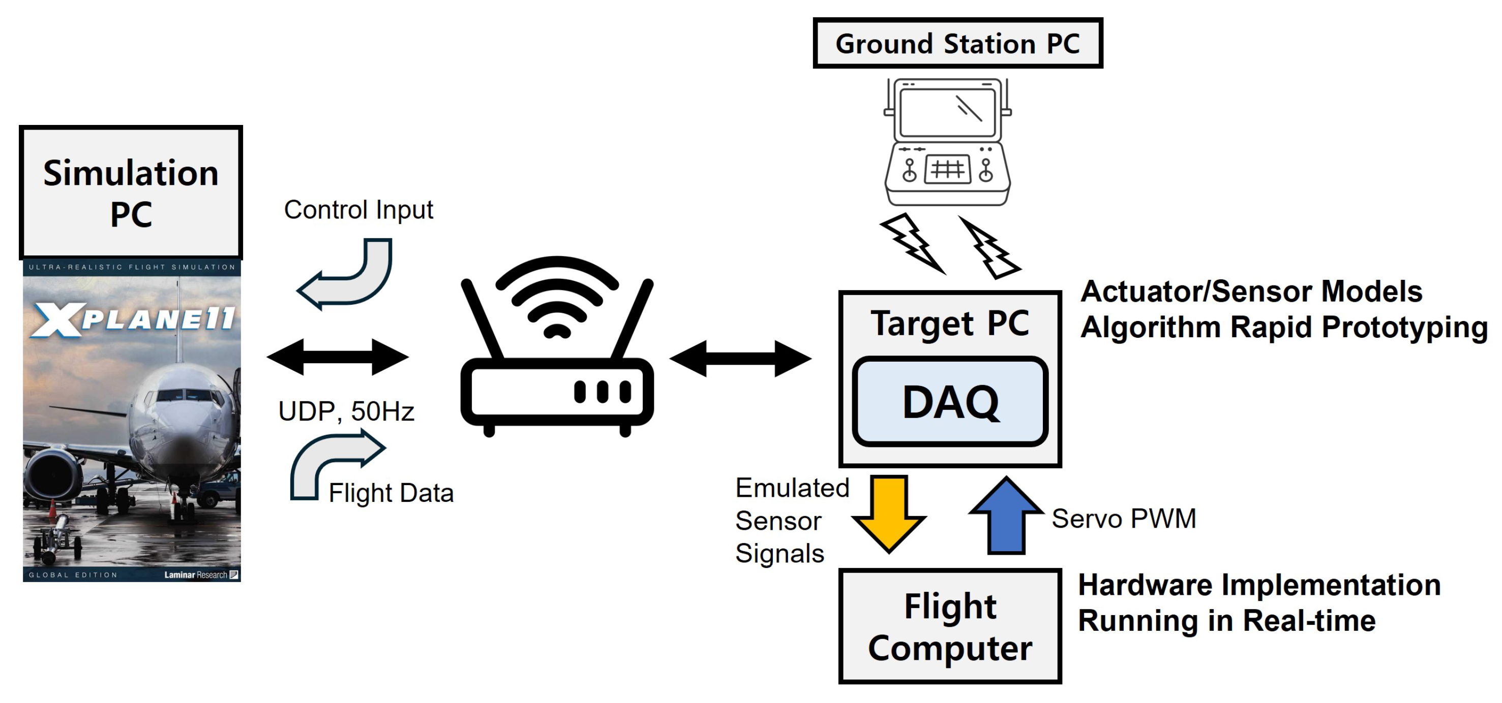
A hardware-in-the-loop simulation environment was developed in-house to validate the proposed UAS guidance algorithm utilizing Matlab® and the Simulink® environment. The system architecture of the HILS environment is depicted in Figure 5. The key component of the system is the target computer on which simulation is being executed in real-time. Running the real-time kernel by Mathworks, the target computer plays an important role in managing the data interface among the simulation computer and the autopilot micro-controller. A high fidelity 6-DOF model of fixed-wing UAS is implemented on the simulation computer via a commercial flight simulator, X-plane by Laminar Research, simulating the dynamic behavior of a fixed-wing UAS along with the command input to control surfaces provided by the target computer. The autopilot has the responsibility of implementing actual flight control algorithms including guidance, navigation, and control. It should be noted that the autopilot also provides the hardware interface to the servo actuators used to deflect the control surfaces of the UAS. The amount of control deflections is obtained by measuring the stroke of the servo actuators via the potentiometers linked to the servo arms. The analog signals from the potentiometers are converted into digital data using two data acquisition boards on the target computer. The target computer feeds the calculated control deflection to the simulator computers as input to the 6-DOF model, which completes the hardware simulation loop. A detailed description of the HILS environment can be found in ref. [32].
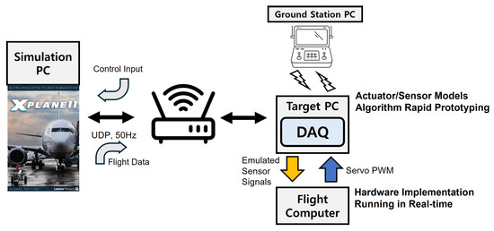
Figure 5.
HILS architecture.
3.2.2. HILS Results
Since the HILS environment makes it possible to verify the seamless integration of both hardware and software by imposing a similar flight condition, the performance of the proposed guidance algorithm is evaluated in various scenarios. A quartic B-spline curve is chosen as a reference path, which is parametrized by a non-decreasing knot vector u. The reference path can be generated using, for instance, the approach in ref. [33], where the reference path is computed using off-line B-spline path templates in accordance with a high-level path planner for obstacle avoidance. Once a B-spline path is given, its geometric features, such as , , and , can be easily computed in terms of the arc-length s.
When calculating the control input in Equation (11), one can use the numerical differentiation of to obtain . However, in order to avoid any high-frequency noise due to differentiation, the approximate value of is obtained by using a differentiation filter with a limiting value. That is, the transfer function , where is used to obtain the approximate value of . The estimation filters and low-level control loops are properly tuned a priori, so only the control gains for the guidance logic need to be carefully chosen accordingly. Table 1 shows the control gains and the simulation parameters.

Table 1.
Control gains for HILS.
First, the path-following performance in terms of parameter adaptation is examined. The simulation results are shown in Figure 6 and Figure 7. When an initial guess of the time constant is inaccurately known (specifically, lower than the true value), it follows from Equation (18) that the commanded roll angle may not be able to generate the equivalent control action to the kinematic control command (via ). Subsequently, this results in a sluggish and low damped response, as shown in Figure 6.

Figure 6.
Error states and command input without parameter adaptation.
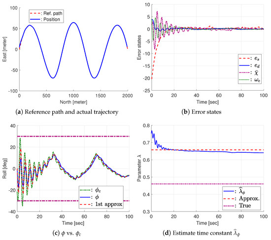
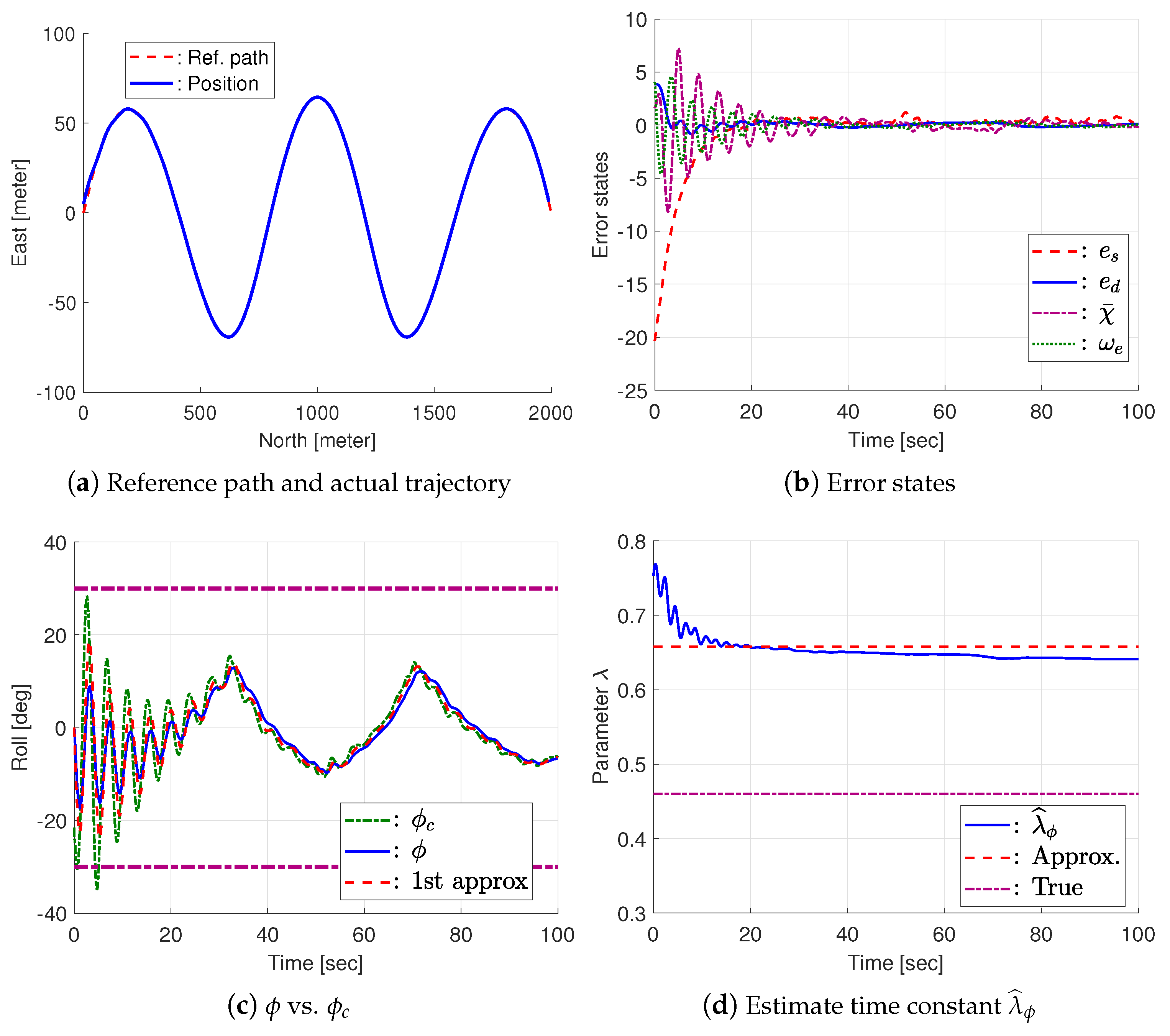
Figure 7.
Error states and command input with parameter adaptation.
With parameter adaptation, the roll angle command is calculated using Equation (18) with the update law of Equation (24) from the large initial guess . Figure 7 shows the results. It should be noted that the error states converge to zero after the initial deviation. The oscillatory response in the initial transient phase is attributed to the large estimate of ; however, as the estimated value approaches the actual values with the parameter adaptation, the errors are well dampened out, resulting in better tracking performance. Figure 7d shows the history of the estimated value of the time constant. The dashed-dot line shows the actual value of the time constant of the low-level roll control loop, while the dashed line represents the time constant computed a posteriori using the data set from Figure 7c. The time constant determines the performance of the roll closed loop system, with larger values leading to a slower response and smaller values resulting in a faster response. Subsequently, although the initial parameter differs from the actual one or is time-varying, the parameter adaptation law readily adjusts the effectiveness of the guidance control logic. As shown in Figure 7d, although it appears that is unable to converge to the true value, the estimated parameter is effectively changed to achieve a satisfactory overall performance.
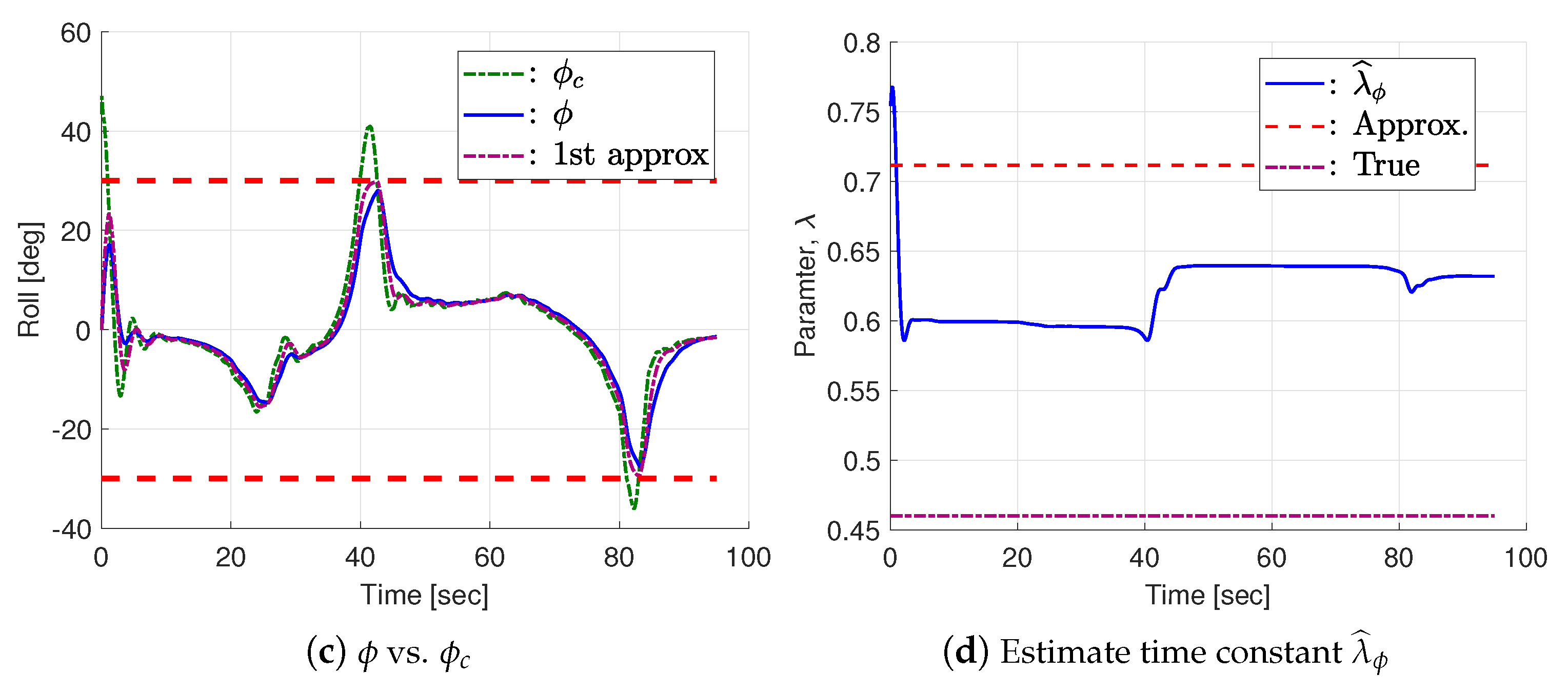
Next, for the sake of more realism during implementation, the simulated roll command was restricted within a prescribed bound. The bound ensures that the assumption of a small roll angle remains valid while also ensuring the safe operation of the fixed-wing UAS by preventing sideslip stall from a large roll angle. However, this bound places a limit on the turning capability of the UAS in terms of the allowable path curvature. Subsequently, the UAS cannot exactly follow a path in which the curvature exceeds the maximum value achievable by the UAS at the given speed. In this study, a roll command limit of [rad] is chosen at a cruising speed of 20 [m/s]. The performance of the path-following control when imposing the roll command limit is shown in Figure 8. As can be shown in Figure 8b, the trajectory of the UAS deviates from the reference path during the sharp left turn, but then the path-following control law enables the UAS to quickly return to the designated path after a while. Figure 8c shows the restricted response of the roll angle due to command saturation. It appears from Figure 8c,d that the restrained roll response at around [s] causes the parameter estimate to jump in the opposite direction of the actual value. A detailed discussion of this phenomenon, along with a possible strategy to mitigate it, is given in the following section.
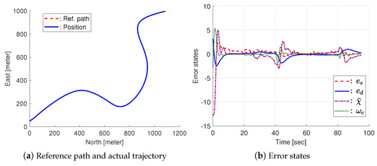
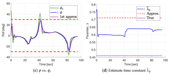
Figure 8.
Error states and command input with parameter adaptation.
3.2.3. Modified Path-Following Control Strategy for Bounded Control Input
In the previous section, the computed roll angle command was given to the inner loop controller by deliberately saturating its amplitude. In practice, this is a straightforward way to drive the roll angle within a safe region. However, as shown in Figure 8d, saturation interferes with the adaptation process, resulting in an inconsistent estimate. Note that when the roll control input is restricted, the errors (including the error of the heading rate ) remain large due to insufficient control authority. As a result, the update law in Equation (24) forces the time constant to increase. To eliminate this unsatisfactory estimate process, a simple yet effective remedy is presented to improve the parameter adaptation process, to cope with roll saturation.
The main idea is to shape the desired kinematic control in Equation (6a) in accordance with the given bound of the roll angle. To this end, suppose that the roll angle bound is given by . The turning rate of the vehicle at a constant forward flight speed is limited by
By the maximum value of the turning rate, the kinematic controller of Equation (6a) is to be bounded as follows:
It should be noted that with the bounded heading rate in Equation (29), the roll command could remain within a certain bound. However, the bounded heading rate is unable to explicitly constrain the roll angle; compared to directly limiting the roll command, it still lacks the ability to explicitly constrain the roll angle. Instead, the benefit of bounding the kinematic control lies in its ability to maintain consistent parameter adaptation. To see this, as shown in Figure 8d, when the roll command is restricted, the large error resulting from insufficient control authority results in an inconsistent estimate. To avoid this, the parameter update needs to become inactive as the vehicle is driven to the maximum turning rate. With the bounded kinematic control , the heading error state becomes
Consequently, a value of near zero causes to remain unchanged (see Equation (24)), which effectively prevents the parameter from growing beyond its acceptable range. A direct consequence of this scheme is that the estimate of the time constant will remain bounded, and thus the path-following control will be insensitive to disturbances, while ensuring a smooth transient.
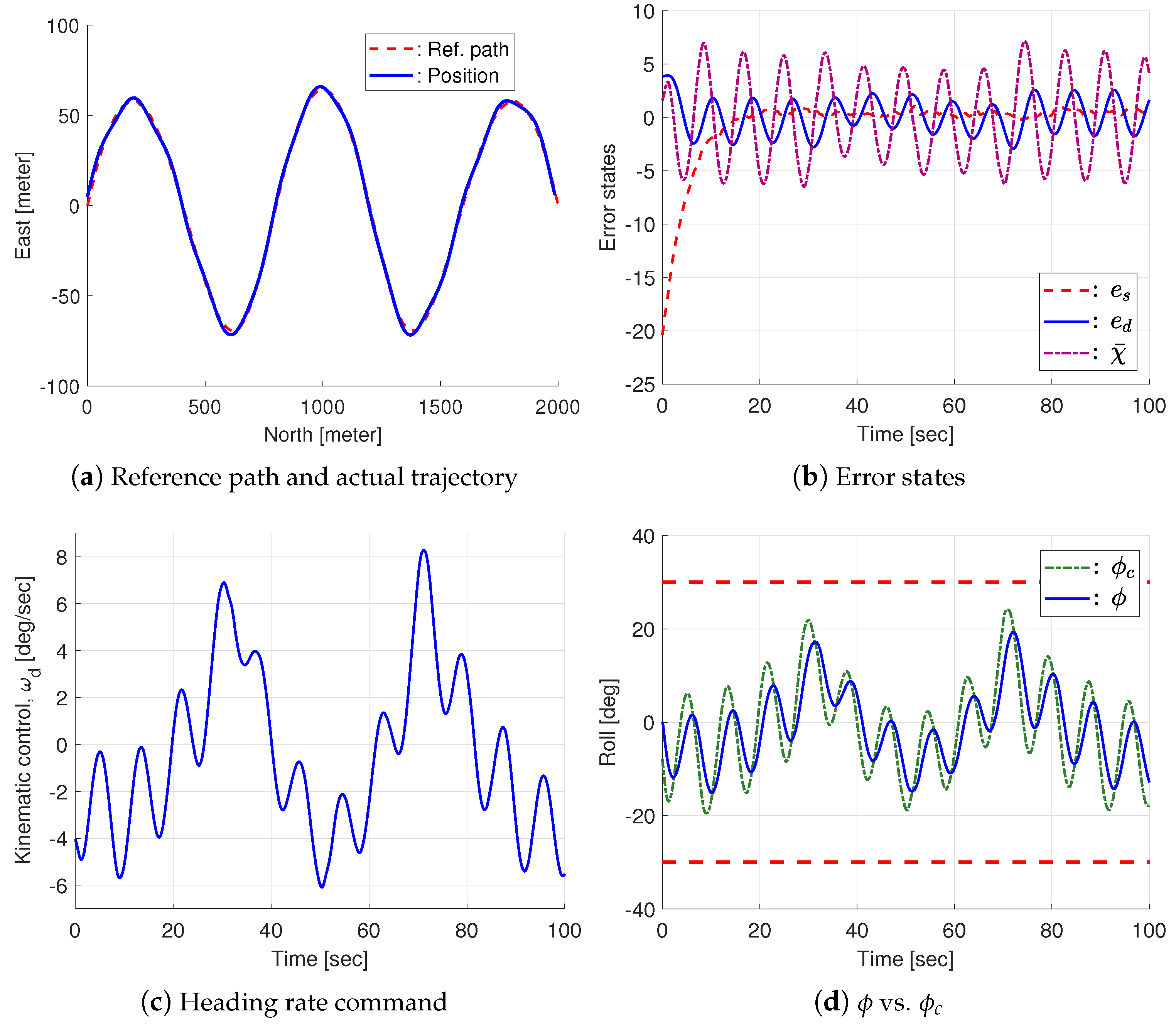
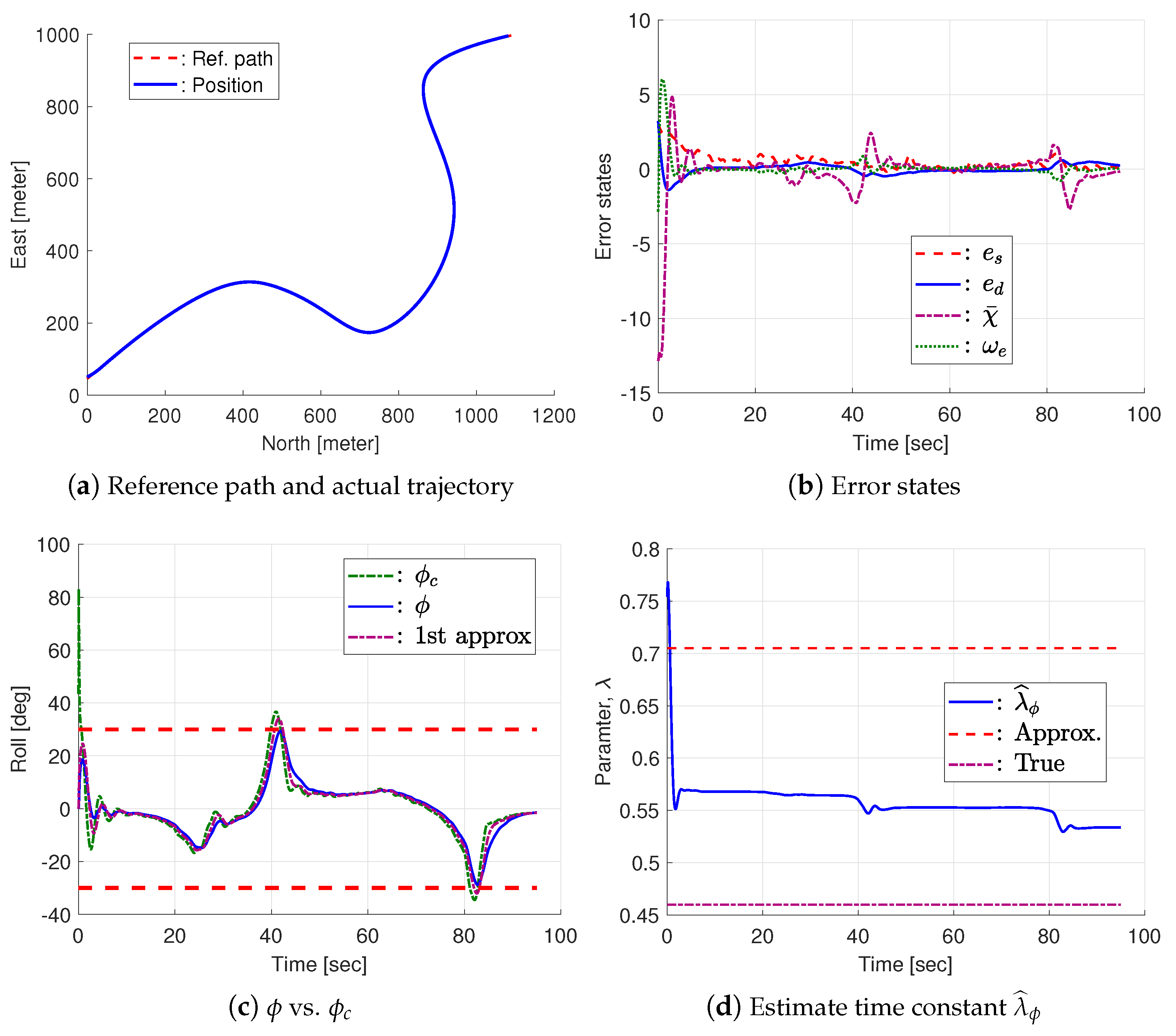
A comparative simulation of the path given in Figure 8 is carried out to demonstrate the performance of this bounding scheme. Figure 9 shows the simulation results. The performance of the parameter estimation has been improved over the previous case, as the unusual growth of the parameter estimate has disappeared. In addition, the proposed bounding scheme has the advantage of fully utilizing kinematic control up to the corresponding maximum roll angle. This is clearly seen in Figure 9c such that the roll angle rapidly approaches its bound when compared to Figure 8c, thus indicating increased control authority.
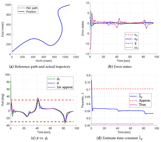
Figure 9.
Error states and command input with parameter adaptation ().
3.3. Performance Validation via Flight Test
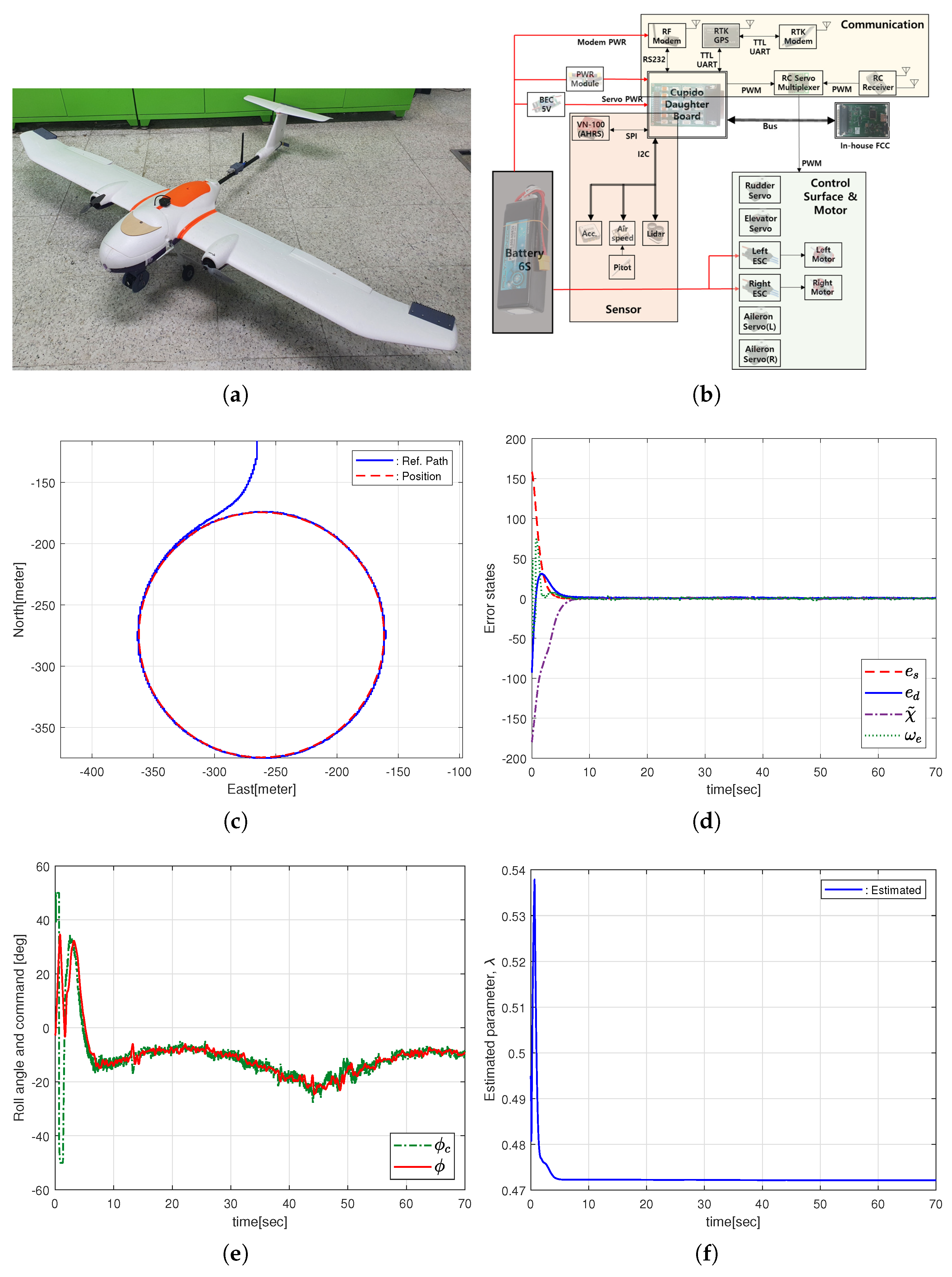
This section describes the performance validation of the proposed guidance algorithm on the actual fixed-wing UAV platform. The experimental platform was built using the commercial R/C airframe, Skywalker Eve-2000, as shown in Figure 10a. The specifications of the platform are summarized in Table 2. The overall avionics system is shown in Figure 10b. The core of the avionics system is the custom autopilot built in-house by the Unmanned Systems Control Lab (USCL) at Korea Aerospace University. The autopilot interfaces with sensors such as the AHRS VN-100 by VectorNAV, RTK GPS receiver Reach M+ by Emlid, airspeed sensor, barometric altimeter, and laser altimeter. The RTK GPS receiver provides a very accurate position fix with a maximum error of 5 cm. The flight control computer computes the high-throughput navigation data via an extended Kalman filter by combining the inertial measurement data from the AHRS and the position and velocity measurement from the RTK GPS. The autopilot implements the proposed guidance and control algorithm as well as the low-level autopilot functions, generating commands for the control surfaces. The details regarding the avionics system of the UAV platform are explained in ref. [34]. The UAV flies at the reference altitude of 100 m above ground level, while the reference airspeed of the UAV is set to 15 m/s. The gain parameters of the proposed guidance law should have been determined with consideration of the optimal performance of the closed-loop system; however, the actual gains were carefully determined through pre-flight tests based on the parameter values chosen from the HILS results, as shown in Table 3.
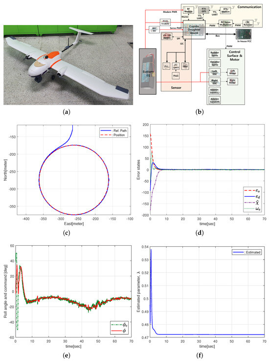
Figure 10.
Error states and command input with parameter adaptation [Flight Test: Case I]. (a) UAV test-bed platform(Skywalker Eve-2000). (b) Architecture of the flight control system [34]. (c) Reference path and actual trajectory. (d) Error states. (e) vs. . (f) Estimate time constant .
Table 2.
Test-bed specification.
Table 3.
Control gains for flight test.
The performance of the proposed guidance algorithm was validated for various trajectory paths. A circular trajectory, given as
where s is the arc-length parameter and is the center of the circle expressed in terms of the Inertial coordinate frame. Note that the radius was set to meters to keep the roll maneuver of the UAV within a sufficiently small range during the coordinated turn.
The experimental results are illustrated in Figure 10c where the blue solid line represents the reference path and the red dashed line represents the actual trajectory flown by the UAV. As the guidance control is invoked from the initial position at meters, Figure 10d shows the convergence of error states towards zero from the initial errors, demonstrating satisfactory tracking performance. In the steady state, the cross-track and the along-track errors remain within approximately m, and the course error stays within about degrees. Figure 10e compares the actual roll angle to the commanded roll. Due to the initial large cross-track error, the roll command is given at its maximum limit; however, by the bounded roll command scheme, the actual roll command effectively remains within the bounded range. Note that there exists roll command variation in accordance with the relative UAV position on the circle. This is attributed to the existence of wind disturbance. That is, when the UAV is located at the West point on the circle, the shallow roll command is enough to keep the UAV on the circle with the help of the West wind. In contrast, when the UAV is located at the East point on the circle, the deep roll command is necessary to overcome the wind disturbance and move towards the circular path. Finally, Figure 10f shows the result of the parameter adaptation law. The history of the estimated time constant of the roll dynamics is shown from the initial guess . It should be noted that after the initial transient, the estimated parameter converges towards near the true value and barely changes. This is because the excitation condition for the adaptation law vanishes over the coordinated turn condition where small heading rate errors prevent the adaptation law from being updated. The gain for the parameter update law can be increased to obtain better estimation results; however, the gain was set to ensure numerical stability, assuming that the bias of the parameter estimation stays within a reasonable range.
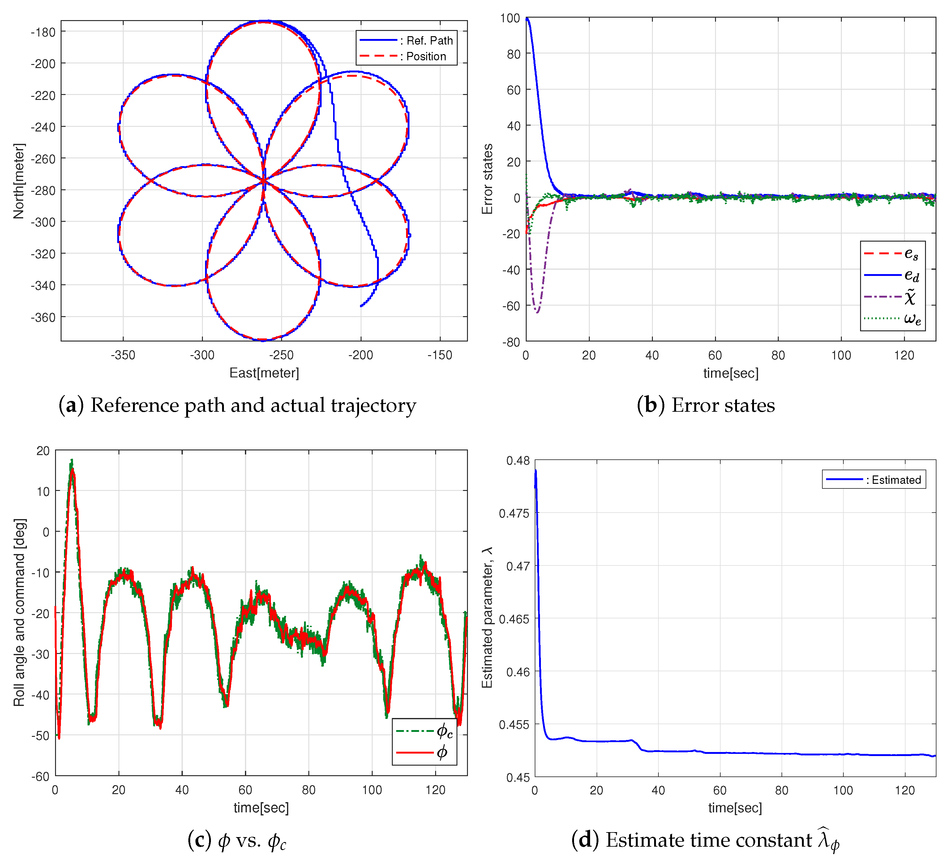
Next, Figure 11 shows the flight test results with a 6-petal geometric path. The path curve is given as,
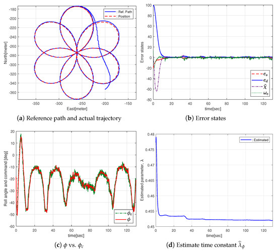
Figure 11.
Error states and command input with parameter adaptation [Flight Test: Case II].
It follows from Figure 11a that the guidance control law makes the UAV successfully follow the path despite the complexity of the path. Due to this complex path, the parameter update law can meet the continuous excitation condition while following the path. As shown in Figure 11d, one can observe that the roll time constant gradually converges to the actual value as the UAV passes each petal of the path curve.
4. Conclusions
A nonlinear path-following control law was developed for a small fixed-wing UAS using backstepping of the course rate command. The kinematic control law implements the cooperative path following, so that the motion of a virtual target is controlled by an extra control input to help the convergence of the error variables. A roll command giving rise to the desired heading rate was derived by taking into account the inaccurate system time constant using parameter adaptation. In addition, a straightforward, yet effective, bounded control scheme is introduced, which ensures that the UAS maneuvers safely within the maximum allowable roll angle. The path-following control algorithm is validated through a high-fidelity hardware-in-the-loop simulation (HILS) environment in various scenarios. Finally, the proposed algorithm was tested experimentally on the actual UAS platform to demonstrate both the tracking performance and control robustness.
Author Contributions
Conceptualization, D.J.; methodology, D.J.; software, S.K.; validation, D.J. and S.K.; formal analysis, D.J.; investigation, S.K.; resources, D.J.; data curation, S.K.; writing—original draft preparation, D.J.; writing—review and editing, S.K.; visualization, S.K.; supervision, D.J.; project administration, D.J.; funding acquisition, D.J. All authors have read and agreed to the published version of the manuscript.
Funding
This work was supported by a 2022 Korea Aerospace University Faculty Research Grant.
Conflicts of Interest
The authors declare no conflicts of interest.
References
- Invernizzi, D.; Giurato, M.; Gattazzo, P.; Lovera, M. Comparison of Control Methods for Trajectory Tracking in Fully Actuated Unmanned Aerial Vehicles. IEEE Trans. Control Syst. Technol. 2020, 29, 1147–1160. [Google Scholar] [CrossRef]
- Willis, J.B.; Beard, R.W. Nonlinear trajectory tracking control for winged eVTOL UAVs. In Proceedings of the 2021 American Control Conference (ACC), New Orleans, LA, USA, 25–25 May 2021; pp. 1687–1692. [Google Scholar]
- Chen, H.; Cong, Y.; Wang, X.; Xu, X.; Shen, L. Coordinated path-following control of fixed-wing unmanned aerial vehicles. IEEE Trans. Syst. Man Cybern. Syst. 2021, 52, 2540–2554. [Google Scholar] [CrossRef]
- Park, S. Rendezvous Guidance on Circular Path for Fixed-Wing UAV. Int. J. Aeronaut. Space Sci. 2021, 22, 129–139. [Google Scholar] [CrossRef]
- Soetanto, D.; Lapierre, L.; Pascoal, A. Adaptive, non-singular Path-following Control of Dynamic Wheeled Robots. In Proceedings of the 42nd IEEE Conference on Decision and Control (CDC), Maui, HI, USA, 9–12 December 20023; pp. 1765–1770. [Google Scholar]
- Liang, X.; Qu, X.; Hou, Y.; Zhang, J. Three-dimensional Path Following Control of Underactuated Autonomous Underwater Vehicle based on Damping Backstepping. Int. J. Adv. Robot. Syst. 2017, 14, 1729881417724179. [Google Scholar] [CrossRef]
- Zhang, Y.; Liu, Y. Guidance-Based Path Following of an Underactuated Ship Based on Event-Triggered Sliding Mode Control. J. Mar. Sci. Eng. 2022, 10, 1780. [Google Scholar] [CrossRef]
- Miao, J.; Sun, X.; Chen, Q.; Zhang, H.; Liu, W.; Wang, Y. Robust Path-Following Control for AUV under Multiple Uncertainties and Input Saturation. Drones 2023, 7, 665. [Google Scholar] [CrossRef]
- Stephan, J.; Pfeifle, O.; Notter, S.; Pinchetti, F.; Fichter, W. Precise Tracking of Extended Three-Dimensional Dubins Paths for Fixed-wing Aircraft. J. Guid. Control Dyn. 2020, 43, 2399–2405. [Google Scholar] [CrossRef]
- Park, S.; Deyst, J.; How, J.P. Performance and Lyapunov Stability of a Nonlinear Path-Following Guidance Method. J. Guid. Control Dyn. 2007, 30, 1718–1728. [Google Scholar] [CrossRef]
- Ren, W.; Beard, R.W. Trajectory Tracking for Unmanned Air Vehicles with Velocity and Heading Rate Constraints. IEEE Trans. Control Syst. Technol. 2004, 12, 706–716. [Google Scholar] [CrossRef]
- Nelson, D.R.; Barber, D.B.; McLain, T.W.; Beard, R.W. Vector Field Path Following for Small Unmanned Air Vehicles. In Proceedings of the 2006 American Control Conference, Minneapolis, MN, USA, 14–16 June 2006; pp. 5788–5794. [Google Scholar]
- Zhang, Z.; He, C.; Chen, H.; Zhang, Y.; Wang, H.; Cai, Y.; Lu, T. Small Fixed-Wing Unmanned Aerial Vehicle Path Following Under Low Altitude Wind Shear Disturbance. IEEE Trans. Intell. Transp. Syst. 2024, 25, 13991–14003. [Google Scholar] [CrossRef]
- Shivam, A.; Ratnoo, A. Arcsine Vector Field for Path Following Guidance. J. Guid. Control Dyn. 2023, 46, 2409–2420. [Google Scholar] [CrossRef]
- Shivam, A.; Ratnoo, A. Vector Field for Following Elliptic Paths. In Proceedings of the AIAA Scitech 2022 Forum, San Diego, CA, USA, 3–7 January 2022. [Google Scholar]
- Wilhelm, J.P.; Clem, G. Vector Field UAV Guidance for Path Following and Obstacle Avoidance with Minimal Deviation. J. Guid. Control Dyn. 2019, 42, 1848–1856. [Google Scholar] [CrossRef]
- Song, Y.; Yong, K.; Wang, X. Disturbance Interval Observer-Based Robust Constrained Control for Unmanned Aerial Vehicle Path Following. Drones 2023, 7, 90. [Google Scholar] [CrossRef]
- Chen, P.; Zhang, G.; Li, J.; Chang, Z.; Yan, Q. Path-Following Control of Small Fixed-Wing UAVs under Wind Disturbance. Drones 2023, 7, 253. [Google Scholar] [CrossRef]
- Zhao, C.; Guo, L.; Yan, Q.; Chang, Z.; Chen, P. Path Tracking Control of Fixed-Wing Unmanned Aerial Vehicle Based on Modified Supertwisting Algorithm. Int. J. Aerosp. Eng. 2024, 2024, 5941107. [Google Scholar] [CrossRef]
- Kumar, S.; Sinha, A.; Kumar, S.R. Robust Path-following Guidance for an Autonomous Vehicle in the Presence of Wind. Aerosp. Sci. Technol. 2024, 150, 109225. [Google Scholar] [CrossRef]
- Nian, X.H.; Zhou, W.X.; Li, S.L.; Wu, H.Y. 2-D Path Following for Fixed Wing UAV using Global Fast Terminal Sliding Mode Control. ISA Trans. 2023, 136, 162–172. [Google Scholar] [CrossRef]
- Reinhardt, D.; Gros, S.; Johansen, T.A. Fixed-Wing UAV Path-Following Control via NMPC on the Lowest Level. In Proceedings of the 2023 IEEE Conference on Control Technology and Applications (CCTA), Bridgetown, Barbados, 16–18 August 2023; pp. 451–458. [Google Scholar]
- Lapierre, L.; Soetanto, D.; Pascoal, A. Nonlinear Path Following with Applications to the Control of Autonomous Underwater Vehicles. In Proceedings of the 42nd IEEE Conference on Decision and Control, Maui, HI, USA, 9–12 December 2003; Volume 2, pp. 1256–1261. [Google Scholar]
- Kaminer, I.; Pascoal, A.; Yakimenko, O. Nonlinear Path Following Control of Fully Actuated Marine Vehicles with Parameter Uncertainty. In Proceedings of the 16th IFAC World Congress, Prague, Czech Republic, 3–8 July 2005; pp. 25–30. [Google Scholar]
- Lapierre, L.; Soetanto, D. Nonlinear Path-Following Control of an AUV. Ocean Eng. 2007, 34, 1734–1744. [Google Scholar] [CrossRef]
- Jung, D. Hierarchical Path Planning and Control of a Small Fixed-Wing UAS: Theory and Experimental Validation. Ph.D. Thesis, Georgia Institute of Technology, Atlanta, GA, USA, 2007. Available online: http://hdl.handle.net/1853/19781 (accessed on 2 November 2024).
- Miao, J.; Wang, S.; Zhao, Z.; Li, Y. Nonlinear Path Following Control of the Underactuated AUV via Reduced-order LESOs and NTD. In Proceedings of the 2016 IEEE International Conference on Aircraft Utility Systems (AUS), Beijing, China, 10–12 October 2016. [Google Scholar]
- Micaelli, A.; Samson, C. Trajectory Tracking for Unicycle-Type and Two-Steering-Wheels Mobile Robots. Ph.D. Thesis, INRIA, Chesnay, France, 1993. [Google Scholar]
- Spooner, J.T.; Maggiore, M.; Ordóñez, R.; Passino, K.M. Stable Adaptive Control and Estimation for Nonlinear Systems; John Wiley & Sons, Inc.: New York, NY, USA, 1999; ISBN 9780471415455. [Google Scholar]
- Gearhart, W.B.; Schulz, H.S. The function sin x/x. Coll. Math. J. 1990, 21, 90–99. [Google Scholar]
- Ardupilot. L1 Controller. Available online: https://github.com/ArduPilot/ardupilot/tree/master/libraries/AP_L1_Control (accessed on 4 October 2024).
- Kang, D.; Kim, S.; Jung, D. Real-time Validation of Formation Control for Fixed-wing UAVs using Multi Hardware-in-the-loop Simulation. In Proceedings of the 2019 IEEE 15th International Conference on Control and Automation (ICCA), Ediburgh, UK, 16–19 July 2019; pp. 590–595. [Google Scholar]
- Jung, D.; Tsiotras, P. On-Line Path Generation for Unmanned Aerial Vehicles Using B-Spline Path Templates. J. Guid. Control Dyn. 2013, 36, 1642–1653. [Google Scholar] [CrossRef]
- Kim, S.; Cho, H.; Jung, D. Evaluation of Cooperative Guidance for Formation Flight of Fixed-wing UAVs using Mesh Network. In Proceedings of the 2020 IEEE International Conference on Unmanned Aircraft System (ICUAS), Athens, Greece, 1–4 September 2020. [Google Scholar]


Disclaimer/Publisher’s Note: The statements, opinions and data contained in all publications are solely those of the individual author(s) and contributor(s) and not of MDPI and/or the editor(s). MDPI and/or the editor(s) disclaim responsibility for any injury to people or property resulting from any ideas, methods, instructions or products referred to in the content. |
© 2025 by the authors. Licensee MDPI, Basel, Switzerland. This article is an open access article distributed under the terms and conditions of the Creative Commons Attribution (CC BY) license (https://creativecommons.org/licenses/by/4.0/).