Digital Low-Altitude Airspace Unmanned Aerial Vehicle Path Planning and Operational Capacity Assessment in Urban Risk Environments

Abstract

This paper proposes a digital low-altitude airspace unmanned aerial vehicle (UAV) path planning method tailored for urban risk environments and conducts an operational capacity assessment of the airspace. The study employs a vertical–horizontal grid partitioning technique to achieve airspace grid-based modeling, classifying and configuring “management-operation” grids. By integrating multi-source heterogeneous data, including building structures, population density, and sheltering factor, a grid-based discrete risk quantification model is established to evaluate comprehensive mid-air collision risk, ground impact risk, third-party risk, and UAV turning risk. A path planning method considering the optimization of the turning points of parallelograms was proposed, and the Parallel-A* algorithm was adopted for its solution. Finally, an airspace operational capacity assessment model and a conflict simulation model for urban risk environments are developed to quantify the operational capacity of urban low-altitude airspace. Using Liuhe District in Nanjing as the experimental area, the study reveals that the environmental airspace risk decreases significantly with increasing flight altitude and eventually stabilizes. In the implementation of path planning, compared with the A* and Weight-A* algorithms, the Parallel-A* algorithm demonstrates clear advantages in terms of lower average comprehensive risk and fewer turning points. In the operational capacity assessment experiments, the airspace capacity across different altitude layers increases with flight altitude and stabilizes after comprehensive risk is reduced. This research provides a theoretical foundation for the scientific management and optimal resource allocation of urban low-altitude airspace, facilitating the safe application and sustainable development of UAVs in urban environments.

1. Introduction

The rapid advancement of urban air mobility (UAM) has led to a growing demand for UAV operations in logistics delivery [1,2,3], emergency response [4,5,6], and inspection tasks [7,8], highlighting the urgent need for airspace fine management in low-altitude environments. Given the challenges posed by multi-source risk coupling, dynamic obstacle interference, and flight efficiency constraints in complex urban low-altitude airspace, establishing a scientifically sound airspace risk assessment framework and achieving safe and efficient path planning have become critical bottlenecks restricting the sustainable utilization of low-altitude resources and the development of intelligent aviation systems.

1.1. Related Prior Work

This section will conduct a review on digital grid airspace modeling, risk assessment, path planning, and airspace capacity assessment. The specific references are listed in Table 1.

In the field of low-altitude digital grid airspace modeling, researchers have established a hierarchical and discretized management foundation. Early studies, such as the AirMatrix 3D air route network [9] proposed by Nanyang Technological University, realized the quantification of airspace capacity and throughput analysis. The grid partitioning scheme based on GeoSOT [10], utilizing a hierarchical encoding mechanism, has facilitated the establishment of dynamic geofences [11] and the detection of flight conflicts [12]. Essentially, the airspace grid system constructs a digital twin of urban airspace, where this discrete representation transforms continuous airspace into addressable computational units. This transformation provides a fundamental foundation for UAV path planning and conflict prediction while serving as a prerequisite for quantifying low-altitude airspace risks.

Low-altitude digital grid airspace modeling offers a spatial framework for the superimposed computation of multidimensional risk fields, driving the evolution of risk assessment methods from traditional collision analysis to multidimensional risk frameworks. Modern approaches decouple risk factors into mid-air collision risk [13,14,15,16,17], ground impact risk [13,14,15,17,18] and third-party risk [16,17]. Airspace grid modeling also facilitates the generation of risk maps, as each grid unit can store and map multiple risk factors. This capability provides an effective tool for UAVs in solving path planning problems, enhancing both safety and operational efficiency.

Based on the risk assessment framework, UAV path planning serves as a strategic bridge between airspace resource management and flight mission execution, with its optimization design directly determining the overall efficiency of low-altitude operational systems. The A* algorithm [19] is a classical path planning method that can identify the optimal route without requiring a complete traversal of the entire grid map. To incorporate risk considerations into path planning, the weighted A* algorithm was introduced [3,20], enabling planned routes to avoid airspace grids with high risk. However, this risk avoidance often results in an increased number of turning points along the planned trajectory. A common approach to mitigating excessive turning points is path smoothing [21,22]. However, trajectory smoothing only softens the boundaries of route inflection points without fundamentally reducing the number of UAV turns, meaning that the risks associated with UAV maneuvers persist.

As a critical component of airspace fine management, airspace capacity assessment is deeply interwoven with the aforementioned grid-based modeling and risk assessment framework. In the field of low-altitude airspace capacity evaluation, researchers have systematically explored strategies for enhancing UAV operational efficiency, safety, and overall system performance through simulation analysis [23,24], topological analysis [25], and modeling optimization [26,27]. Simulation methods [23,24] have played a crucial role in these studies by providing a controlled airspace simulation environment. Through the definition of airspace capacity as the minimum air traffic volume at which phase transitions occur in airspace evaluation metrics (such as conflict rate), simulation-based approaches have established a theoretical foundation for the quantitative analysis of low-altitude airspace capacity.

Table 1. Relevant work of digital grid airspace modeling, risk assessment, UAV path planning, and airspace capacity assessment.

Type	Paper	Method and Study	Core Contribution
Digital grid airspace	Mohamed Salleh et al. [9]	AirMatrix	Propose the implementation of AirMatrix three-dimensional airway network for the quantitative analysis of airspace capacity and throughput.
	Xu et al. [10]	GeoSOT	Introduce the hierarchical coding mechanism of grid partitioning for GeoSOT.
	Tang et al. [11]	GeoSOT	Research on Dynamic Geographical Fence Establishment Based on GeoSOT.
	Shi et al. [12]	GeoSOT	Carry out flight conflict detection based on GeoSOT.
Risk assessment	Martin et al. [13]	Mid-Air Collision Risk, Ground Impact Risk	A set of procedures for managing the risk assessment of UAVs in both mid-air collision risk and ground impact risk.
	Civil Aviation Administration of China (CAAC) [14]	Mid-Air Collision Risk, Ground Impact Risk	Provide ground impact risk and mid-air collision risk assessment services for CAAC, operation responsible persons of specific types of unmanned aircraft to be operated, service providers of air traffic management and other relevant third parties.
	Shao et al. [15]	Mid-Air Collision Risk, Ground Impact Risk	Conduct risk assessment of mid-air collision risk and ground impact risk for UAV logistics delivery scenarios.
	Banerjee et al. [16]	Mid-Air Collision Risk, Third-Party Risk	It elaborated on the possibility of risk associated with obstacle collision and took into account the influence of abnormal conditions introduced by component failures, reduced controllability, and environmental interference.
	Pang et al. [17]	Mid-Air Collision Risk, Ground Impact Risk, Third-Party Risk, Risk Maps	Risk is quantified by using risk maps. The risk assessment model includes risk of death, property loss and noise impact.
	Primatesta et al. [18]	Ground Impact Risk, Risk Maps	Employ risk maps to define the ground risks associated with unmanned aircraft accidents.
UAV path planning	AVGC et al. [19]	Traditional A*	Path planning algorithm based on sampling search.
	Zhang et al. [3]	Weighted A*	Set the risk as the weight to solve the problem of setting up the logistics distribution routes for the “last mile”.
	Zhang et al. [20]	Weighted A*	Establish a risk-based urban airspace environment model, and plan UAVs with low operational risks, low noise levels, and low transportation costs.
	Jung et al. [21]	Path Smoothing	The problem of generating smooth reference paths was raised under the condition that a finite discrete set of local optimal path families was given.
	Wang et al. [28]	Path Smoothing	An improved A* algorithm based on the optimization of key point selection and smooth path generation is proposed. The A* algorithm is combined with Bezier curves to process the smoothness of the generated path.
Airspace capacity assessment	Bulusu et al. [29]	Simulation Analysis	Estimate flight capacity through the assessment of flight conflicts among unmanned aerial vehicles operating in the airspace.
	Starita et al. [24]	Simulation Analysis	Take into account a large number of traffic scenarios to consider the uncertainties of traffic and capacity supply.
	Cho et al. [25]	Topological Analysis	The topology method of setting up access-restricted and exit-restricted geographic fences is adopted for conducting airspace capacity assessment.
	Vascik et al. [26]	Modeling Optimization	A method of integer programming is proposed to analyze and estimate the capacity of vertical take-off and landing airports.
	Zhou et al. [27]	Modeling Optimization	Introduce the traffic dynamics model and solve the capacity of the UAV in both stable and unstable states.

Table 1. Relevant work of digital grid airspace modeling, risk assessment, UAV path planning, and airspace capacity assessment.

Type	Paper	Method and Study	Core Contribution
Digital grid airspace	Mohamed Salleh et al. [9]	AirMatrix	Propose the implementation of AirMatrix three-dimensional airway network for the quantitative analysis of airspace capacity and throughput.
	Xu et al. [10]	GeoSOT	Introduce the hierarchical coding mechanism of grid partitioning for GeoSOT.
	Tang et al. [11]	GeoSOT	Research on Dynamic Geographical Fence Establishment Based on GeoSOT.
	Shi et al. [12]	GeoSOT	Carry out flight conflict detection based on GeoSOT.
Risk assessment	Martin et al. [13]	Mid-Air Collision Risk, Ground Impact Risk	A set of procedures for managing the risk assessment of UAVs in both mid-air collision risk and ground impact risk.
	Civil Aviation Administration of China (CAAC) [14]	Mid-Air Collision Risk, Ground Impact Risk	Provide ground impact risk and mid-air collision risk assessment services for CAAC, operation responsible persons of specific types of unmanned aircraft to be operated, service providers of air traffic management and other relevant third parties.
	Shao et al. [15]	Mid-Air Collision Risk, Ground Impact Risk	Conduct risk assessment of mid-air collision risk and ground impact risk for UAV logistics delivery scenarios.
	Banerjee et al. [16]	Mid-Air Collision Risk, Third-Party Risk	It elaborated on the possibility of risk associated with obstacle collision and took into account the influence of abnormal conditions introduced by component failures, reduced controllability, and environmental interference.
	Pang et al. [17]	Mid-Air Collision Risk, Ground Impact Risk, Third-Party Risk, Risk Maps	Risk is quantified by using risk maps. The risk assessment model includes risk of death, property loss and noise impact.
	Primatesta et al. [18]	Ground Impact Risk, Risk Maps	Employ risk maps to define the ground risks associated with unmanned aircraft accidents.
UAV path planning	AVGC et al. [19]	Traditional A*	Path planning algorithm based on sampling search.
	Zhang et al. [3]	Weighted A*	Set the risk as the weight to solve the problem of setting up the logistics distribution routes for the “last mile”.
	Zhang et al. [20]	Weighted A*	Establish a risk-based urban airspace environment model, and plan UAVs with low operational risks, low noise levels, and low transportation costs.
	Jung et al. [21]	Path Smoothing	The problem of generating smooth reference paths was raised under the condition that a finite discrete set of local optimal path families was given.
	Wang et al. [28]	Path Smoothing	An improved A* algorithm based on the optimization of key point selection and smooth path generation is proposed. The A* algorithm is combined with Bezier curves to process the smoothness of the generated path.
Airspace capacity assessment	Bulusu et al. [29]	Simulation Analysis	Estimate flight capacity through the assessment of flight conflicts among unmanned aerial vehicles operating in the airspace.
	Starita et al. [24]	Simulation Analysis	Take into account a large number of traffic scenarios to consider the uncertainties of traffic and capacity supply.
	Cho et al. [25]	Topological Analysis	The topology method of setting up access-restricted and exit-restricted geographic fences is adopted for conducting airspace capacity assessment.
	Vascik et al. [26]	Modeling Optimization	A method of integer programming is proposed to analyze and estimate the capacity of vertical take-off and landing airports.
	Zhou et al. [27]	Modeling Optimization	Introduce the traffic dynamics model and solve the capacity of the UAV in both stable and unstable states.

1.2. Our Contributions

In response to the aforementioned issues, this paper proposes a method for digital low-altitude airspace UAV path planning and operational capacity assessment in urban risk environments. The main contributions of this study are as follows:

(1) By making use of the multi-scale grid partitioning of GeoSOT and through hierarchical encoding, the spatial attributes (such as terrain complexity, physical obstacles, etc.) are mapped to a unified spatial reference. This breaks through the limitation of fixed scale of AirMatrix and enables the leap from single-dimensional management of airspace to multi-attribute coupling management.

(2) Previous approaches to airspace risk analysis only took into account environmental risks (mid-air collision risk, ground impact risk, and third-party risk). Based on the establishment of environmental risk maps, this paper further considers the risk of turning points generated by path planning, achieving a joint analysis of environmental risks and planning risks.

(3) Based on the idea of translation optimization, starting from the path structure itself, the Parallel-A* algorithm is designed to optimize the paths planned by the weighted A* algorithm. It changes the original paths and optimizes the number of inflection points.

(4) By applying the simulation analysis method and integrating the path planning algorithm proposed in this question, the assessment of airspace operation capacity is conducted. The Normalized Time Spent in Conflict ($\mathrm{N}\mathrm{T}\mathrm{S}\mathrm{C}$) is defined as the number of acceptable conflicts, and the airspace operation capacity is calculated.

In response to these challenges, this study first conducts airspace grid-based modeling and classifies “management-operation” grids for urban low-altitude airspace. A grid-based discrete risk quantification model is then developed, integrating mid-air collision risk, ground impact risk, third-party risk, and UAV turning risk. To optimize UAV flight paths, a parallelogram-based turning point optimization path planning method is introduced, minimizing risk and transportation costs, and solved using the Parallel-A* algorithm. Additionally, an airspace operational capacity assessment model and a conflict simulation model tailored to urban risk environments are established to compute airspace operational capacity. Finally, a series of simulation experiments are conducted using Liuhe District in Nanjing as the case study area.

2. Airspace Grid-Based Modeling

The grid partitioning of urban low-altitude airspace is not merely a technical innovation but represents a fundamental shift in airspace management paradigms. By discretizing continuous low-altitude airspace into computationally addressable and quantifiable independent grid units, this approach enables more refined and systematic airspace management for urban environments. This study proposes a vertical–horizontal grid partitioning method, which first performs vertical and horizontal partitioning to construct a 3D airspace grid. Subsequently, the grids are classified into management-scale and operation-scale categories, with their vertical $S_v$ and horizontal dimensions $S_h$ configured accordingly based on classification criteria.

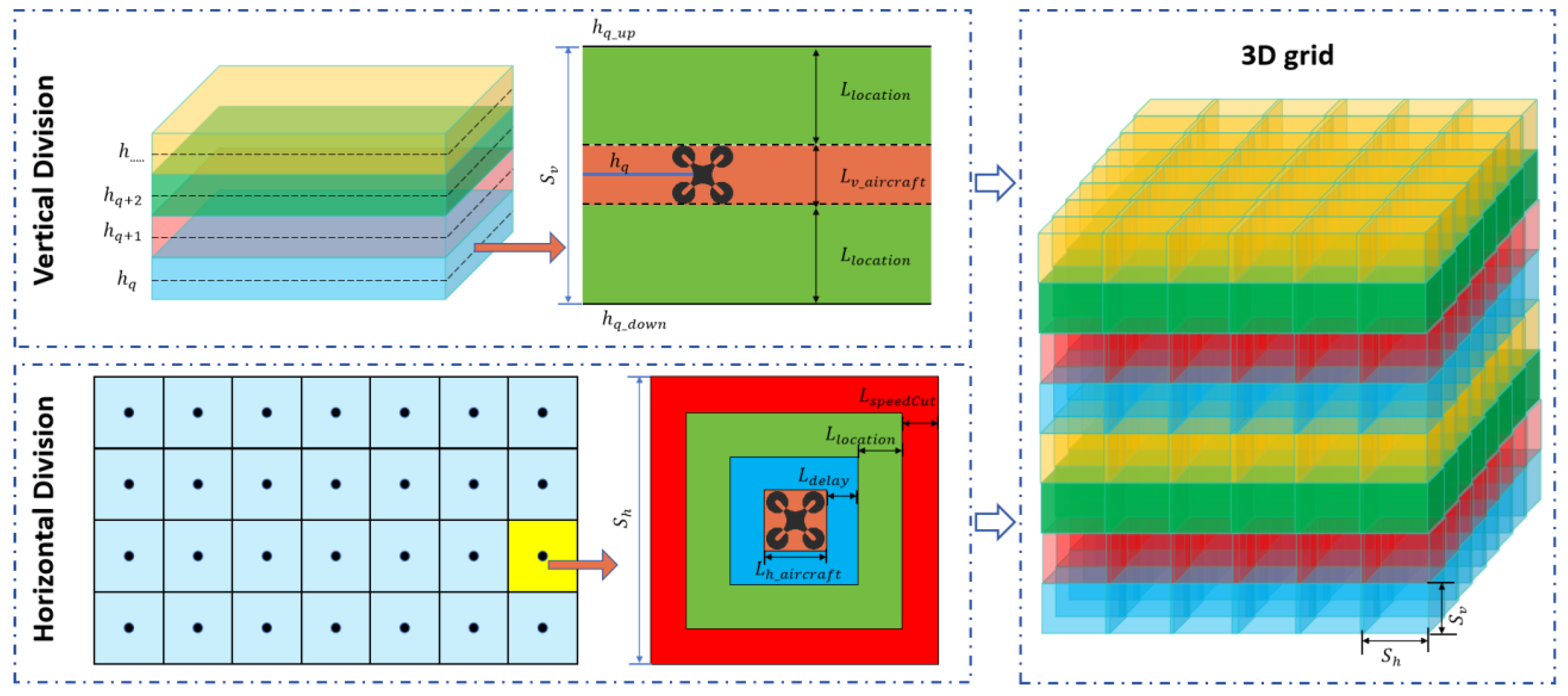
2.1. Vertical–Horizontal Grid Partitioning

2.1.1. Vertical Partitioning

Using mean sea level as the reference plane, the study performs vertical partitioning of the low-altitude airspace within the 0–3000 m range. A vertical partitioning is performed at interval $S_v$, generating a set of horizontal airspace layers $H_{set}$:

$$H_{set}=\{h_1,h_2,\dots ,h_q,\dots \}$$

(1)

where $h_q$ represents the altitude of the $q$-th horizontal airspace layer.

The upper $h_{q\_up}$ and lower $h_{q\_down}$ boundaries of each horizontal airspace $h_q$ layer can be expressed as

$$h_{q\_up}=h_q+{\displaystyle \frac{S_v}{2}}$$

(2)

$$h_{q\_down}=h_q-{\displaystyle \frac{S_v}{2}}$$

(3)

2.1.2. Horizontal Partitioning

Layered flight is a kind of divide and conquer thinking. Through hierarchical management of airspace or tasks, it enables efficient and safe flight planning in complex scenarios and is particularly suitable for multi-aircraft collaboration or high-density airspace scenarios. For horizontal airspace grid partitioning, this study employs a GeoSOT-based approach to partition the horizontal airspace into grids with a side length of $S_h\times S_h$, resulting in a multi-scale hierarchical grid system. GeoSOT grids [30] represent a form of latitude–longitude partitioning grid system, offering seamless compatibility with existing spatial data frameworks.

Table 2. Grid sizes and scales corresponding to various levels in the GeoSOT partitioning method.

Level	Grid Size	Scale	Level	Grid Size	Scale
0	512°		17	16″	512 m
1	256°		18	8″	256 m
2	128°		19	4″	128 m
3	64°		20	2″	64 m
4	32°		21	1″	32 m
5	16°		22	1/2″	16 m
6	8°	1024 km	23	1/4″	8 m
7	4°	512 km	24	1/8″	4 m
8	2°	256 km	25	1/16″	2 m
9	1°	128 km	26	1/32″	1 m
10	32′	64 km	27	1/64″	0.5 m
11	16′	32 km	28	1/128″	25 cm
12	8′	16 km	29	1/256″	12.5 cm
13	4′	8 km	30	1/512″	6.2 cm
14	2′	4 km	31	1/1024″	3.1 cm
15	1′	2 km	32	1/2048″	1.5 cm
16	32″	1 km

presents the grid sizes and scales corresponding to various levels of the GeoSOT partitioning method.

The vertical–horizontal grid partitioning schematic is illustrated in Figure 1.

2.2. Classification and Configuration of “Management-Operation” Grids

2.2.1. Management-Scale Grids

Management-scale grids are configured based on the administrative boundaries of national, provincial, municipal, and district/county-level airspace management regions. These grids are selected from GeoSOT, the partitioning scale system, to form regional management-scale grids, provincial management-scale grids, municipal management-scale grids, and district/county management-scale grids. The parameter $S_v$ can be customized by regional airspace administrators based on the type of airspace management, while $S_h$ can be configured according to specific administrative boundaries at different management levels.

The scale $S_h$ configuration method is as follows:

Step 1: Acquire the point set $P=\{p_1,p_2,\dots ,p_n\}$ defining the contour of a given administrative region, where each $p_i=(x_i,y_i)$ represents a coordinate in a two-dimensional plane.

Step 2: Compute the minimum bounding square of the point set $P$, where the side length of the minimum bounding rectangle is denoted as $d_{square}$.

Step 3: Map $d_{square}$ to the corresponding grid level $n$ of $\mathrm{G}\mathrm{e}\mathrm{o}\mathrm{S}\mathrm{O}\mathrm{T}$. The appropriate grid scale $S_h$ for level $n$ can be determined using Table 2. The corresponding level $n$ is calculated using the following formula:

$$n=⌈{log}_2\left({\displaystyle \frac{2\pi R}{D_{opration}}}\right)⌉$$

(4)

where $R$ represents the Earth’s radius, set as $R\approx 6371000$ m.

This article refers to the “Interim Regulation on the Administration of the Flight of Unmanned Aircraft” issued by The State Council of the People’s Republic of China, Central Military Commission of the People’s Republic of China [31], and divides airspace into controlled airspace and uncontrolled airspace. The definition of controlled airspace is the airspace above an altitude of 120 m or more. The airspace prohibited in the air, the restricted airspace in the air, the surrounding airspace, the ultra-low-altitude flight airspace for military aviation, and some other areas [31] should be designated as controlled airspace. And uncontrolled airspace is the airspace outside the controlled airspace. Therefore, in this paper, the management-scale grids are classified into controlled grids and uncontrolled grids.

2.2.2. Operation-Scale Grids

The operation-scale grid is determined based on UAV performance parameters, communication latency, and positioning errors, collectively defining the operation-scale grid’s $S_v$ and $S_h$.

(1)

Determination of Vertical Grid Scale

$S_v$ can be adjusted according to UAV performance characteristics. This study primarily considers UAV longitudinal dimensions $L_{v\_aircraft}$ and positioning system errors $E_{location}$ in the vertical direction, which can be expressed as

$$S_v=L_{v\_aircraft}+2\times L_{location}$$

(5)

(2)

Determination of Horizontal Grid Scale

The horizontal partitioning method for operation-scale grids comprehensively accounts for key factors such as UAV horizontal dimensions, operational parameters, communication latency, and positioning errors. This approach ensures a rational determination of horizontal grid scale for UAV operations in low-altitude airspace. The horizontal grid partitioning scale is jointly determined by UAV horizontal dimensions $L_{h\_aircraft}$, positioning system errors $L_{location}$, deceleration displacement at maximum velocity $L_{speedCut}$, and communication latency displacement $L_{delay}$, collectively defining the minimum safe separation distance $D_o$ for UAVs, which can be expressed as

$$D_o=L_{h\_aircraft}+2\times (L_{location}+L_{speedCut}+L_{delay})$$

(6)

where $L_{speedCut}$ represents the displacement of a UAV decelerating from its maximum flight speed $V_{max}$ to $0 \mathrm{m}/\mathrm{s}$, calculated as

$$L_{speedCut}={\displaystyle \frac{{V_{max}}^2}{2\times a_{max}}}$$

(7)

where $a_{max}$ represents the maximum deceleration.

The displacement caused by the time delay $t_{trans}$ in transmitting UAV positioning information to the ground control station or air traffic management platform is given by

$$L_{Delay}=t_{trans}\times V_{max}$$

(8)

Using Equation (6), map $D_o$ to the corresponding grid level $n$ of GeoSOT. The appropriate operational-scale grid size $S_h$ for level $n$ can be determined from Table 2.

The vertical–horizontal grid partitioning schematic is illustrated in Figure 2.

The operation-scale grids are divided into two categories: fly-permitted grids and fly-prohibited grids. Fly-permitted grids are those areas within the airspace where UAVs are allowed to enter. Fly-prohibited grids, on the other hand, refer to regions in the airspace where UAVs are prohibited from entering. Fly-prohibited grids mainly include areas such as communication signal blind spots, physical obstacles, buildings, government and military key areas, and special event zones.

3. Discrete Quantitative Risk Assessment Model for Urban Low-Altitude Airspace Grids

The risk assessment of urban low-altitude airspace integrates multi-source heterogeneous data, including urban 3D geographic information, population density, physical obstacles, and UAV parameters, to construct a grid-based discrete quantitative risk assessment model. At its core, this model maps multidimensional risk attributes to individual grid units, generating a low-altitude urban airspace risk heatmap. This study primarily evaluates risk from four perspectives: mid-air collision risk, ground impact risk, third-party risk and UAV turning risk.

3.1. Mid-Air Collision Risk

Mid-air collision risk primarily considers the probability of UAVs colliding with physical obstacles during flight. This study employs the artificial potential field method to assign repulsive forces to physical obstacles [32], where the mid-air collision risk $U_f^i$ exerted by an obstacle grid $f$ for grid $i$ can be expressed as

$$U_f^i=\left\{\begin{array}{ll}{\displaystyle \frac{a_f}{2}}\times {({\displaystyle \frac{1}{d_f^i}}-{\displaystyle \frac{1}{d_0}})}^2,& d_f^i\le d_f\\ 0,& d_f^i\ge d_f\end{array}\right.$$

(9)

where $d_f^i$ represents the Euclidean distance between $i$ and $f$. $a_f$ denotes the potential field parameter of $f$, and $d_f$ is the radiation distance threshold of the mid-air collision risk potential field for $f$.

According to Equation (9), the smaller $d_f^i$ is, the larger $U_f^i$ becomes, which increases the risk of mid-air collisions generated by $f$; conversely, the larger $d_f^i$ is, the smaller $U_f^i$ becomes, reducing the airborne collision risk associated with $f$. It further explains that the distance between the grid and the physical obstacles shows a negative correlation. Based on this characteristic, the risk of air collision caused by the grid of physical obstacles can be quantified. Specifically, when $f$ itself is 1, $U_f^i=1$; for its 1st-order neighborhood grid, $U_f^i=0.5$; for the 2nd-order neighborhood grid, $U_f^i=0.25$; and for the else grids, $U_f^i=0$. As shown in Figure 3.

The quantified risk of mid-air collision can be expressed as

$$U_f^i=\left\{\begin{array}{c}\begin{array}{cc}1& i\in {set}_{own}^f\end{array}\\ \begin{array}{cc}0.5& i\in {set}_{1st}^f\end{array}\\ \begin{array}{cc}0.25& i\in {set}_{{set}_{2nd}^f}\end{array}\\ \begin{array}{cc}0& i\in {set}_{{set}_{3th}^f}\end{array}\end{array}\right.$$

(10)

In environments with a high density of obstacles, grid $i$ may simultaneously be affected by mid-air collision risks from multiple physical obstacles. Therefore, the mid-air collision risk $R_{obstacle}^i$ experienced by grid $i$ is the cumulative effect of the collision risks exerted by all surrounding physical obstacles, which can be expressed as

$$R_{collision}^i=sum\left({set}_{U_f}^i\right)$$

(11)

where ${set}_{U_f}^i$ represents the set of mid-air collision risks exerted by physical obstacles on grid $i$, and $sum\left({set}_{U_f}^i\right)$ denotes the summation function.

Finally, the mid-air collision risk of the $h_q$ layer grid can be calculated through Formula (11), and the risk set ${set}_{collision}$ can be obtained. Furthermore, all $R_{collision}^i$ in the set need to be subjected to $min-max$ normalization processing through Formula (11), which is as follows:

$$Q\prime (x)={\displaystyle \frac{Q\left(x\right)-{Q\left(x\right)}_{min}}{{Q\left(x\right)}_{max}-{Q\left(x\right)}_{min}}}$$

(12)

where $Q\prime \left(x\right)$ represents the normalized sub-cost value, $Q\left(x\right)$ denotes the actual sub-cost value, and ${Q\left(x\right)}_{min}$ and ${Q\left(x\right)}_{max}$ correspond to the minimum and maximum sub-cost values, respectively.

3.2. Ground Impact Risk

In this study, ground impact risk refers to the potential threat posed by UAV operations to human safety on the ground. The ground impact risk for a given grid $i$ can be expressed as [3]

$$R_{crash}^i=N_{people}^i\times En\times (1-G_S^i)\times P_{uav}$$

(13)

where $N_{people}$ represents the number of individuals in the impact zone during a UAV crash event; $G_S$ is the occlusion factor of the grid, reflecting the exposure level of individuals to UAV operations. The values of the sheltering factor are provided in

Table 3. Sheltering factor values.

Values	Classification
0.00	No obstacles
0.25	Sparse trees
0.50	Vehicles and low-rise buildings
0.75	High buildings
1.00	Industrial buildings

. $E_n$ denotes the kinetic energy of UAV impact [18], calculated as

$$E_n=m_{all}g{h}_q+0.5m_{all}{v}^2$$

(14)

where $m_{all}$ represents the total mass of the UAV at the time of impact, which includes both the UAV’s own weight $m_{uav}$ and the payload weight $m_{cargo}$, that is ${m_{all}=m}_{uav}+m_{cargo}$. In this study, the maximum take-off weight of the UAV is used for $m_{all}$. $v$ represents the flight speed. $P_{uav}$ represents the crash probability, which can be expressed as

$$P_{uav}={\displaystyle \frac{1}{1+\sqrt{\frac{\alpha }{\beta }{\left[\frac{\beta }{E_{imp}}\right]}^{\frac{1}{4\times G_S}}}}}={\displaystyle \frac{1}{1+\sqrt{\frac{\alpha }{\beta }{\left[\frac{\beta }{0.5{\times m}_{all}\times v_{imp}^2}\right]}^{\frac{1}{4\times G_S}}}}}$$

(15)

where $\alpha$ represents the impact energy causing a 50% fatality rate when $G_S=$ 0.5; $\beta$ denotes the impact energy threshold causing human casualties when $G_S\to 0$; $E_{imp}$ is the impact energy at the UAV crash site; $v_{imp}^2$ is the impact velocity, which can be expressed by the following formula:

$$v_{imp}^2=v_x^2+v_y^2=v_x^2+\sqrt{{\displaystyle \frac{2(m_{uav}+m_{cargo})}{\rho C_d{A}_{drop}}}+[1-exp{\displaystyle \frac{-h_q\rho C_{d}A}{m_{all}}}]}$$

(16)

Finally, using Equation (13), the risk set ${set}_{crash\_risk}$ for $h_q$ layer is calculated, with all $R_{crash}^i$ within the set normalized using Equation (12).

3.3. Third-Party Risk

Third-party risk primarily considers the risk associated with noise pollution generated by UAV operations. Noise risk refers to the impact of UAV noise on urban residents, necessitating measures to minimize disturbance during urban airspace operations. Noise risk is influenced by three key factors [3]: (1) Noise source, the acoustic energy emitted by UAV propellers during flight. (2) Sound barriers, the ability of obstacles between the UAV and the noise receptor to attenuate sound propagation. (3) Exposure, the number of individuals affected by UAV noise. The noise risk for a given grid can be defined as [33]

$$R_{noise}^i=HA\%\times (1-0.8{G_S}_i)\times A_i\times N_{people}^i$$

(17)

where $L$ represents the noise factor; $A_i$ denotes the horizontal grid area, calculated as $S_h\times S_h$; $HA\%$ is the residential annoyance index, expressed as

$$HA\%={\displaystyle \frac{123.81}{1+exp(9.99-0.15(L_{uav}-∆L\left)\right)}}$$

(18)

where $L_{uav}$ represents the sound intensity level emitted by the UAV source; $∆L$ denotes the attenuation of noise, which is dependent on the distance between residents and the UAV flight path, formulated as

$$∆L=10\times lg(0.25\times \pi \times h)$$

(19)

where $h$ is the distance between residents and the UAV flight trajectory.

Similarly, using Equation (17), the risk set ${set}_{noise\_risk}$ for grid $h_q$ layer is calculated, with all $R_{noise}^i$ normalized using Equation (11).

3.4. UAV Turning Risk

During UAV flight operations, changes in orientation or turning maneuvers result in energy loss and increased operational risk [34]. To address this, this study defines the UAV turning risk, which quantifies the impact of directional changes on flight safety. Assuming that a UAV performs a turning maneuver while traversing a grid $i$, the turning risk associated with grid $i$ is defined as

$$R_{turn}^i={\displaystyle \frac{{\delta }_i}{{\delta }_{safe}\times R_{max}^i}}$$

(20)

where ${\delta }_i$ represents the turning angle, ${\delta }_{safe}$ denotes the safe turning angle, ${\delta }_{safe}=45°$ which is predefined based on urban environmental constraints, and $R_{max}^i$ is the maximum turning risk, which can be determined according to the maximum allowable turning angle of the UAV, expressed as

$$R_{max}^i={\displaystyle \frac{{\delta }_{max}}{{\delta }_{safe}}}$$

(21)

where ${\delta }_{max}$ represents the maximum turning angle of the UAV.

3.5. Comprehensive Risk

Based on the above risk analysis, the four types of risks can be classified into environmental risks and planning risks. Environmental risks refer to the environmental factors that are planned before the flight path of the UAV, mainly including risks of mid-air collision, ground impact, and third-party risks; planning risks mainly include the turning risks of the UAV during the flight process. The turning risks and planning risks can be expressed as follows:

$$E_i=w_1\times R_{collision}^i+w_2\times R_{crash}^i+w_3\times R_{noise}^i$$

(22)

$$W_i=R_{turn}^i$$

(23)

where $w_1$, $w_2$, and $w_3$ represent the weights corresponding to the risks of mid-air collision, ground impact, and third-party risk, respectively, and $w_1+w_2+w_3=1$.

From the above, it can be known that environmental risks are pre-existing risks before path planning, while planning risks mainly include the turning risks of the UAV during flight, and the path risks after the UAV’s path planning is completed. Therefore, in this paper, the sum of the pre-existing environmental risks with the planning risks generated after path planning is taken as the comprehensive risk, which can be expressed as

$$R_i=E_i+W_i$$

(24)

4. Parallelogram-Based Turning Point Optimization Path Planning Method

To optimize UAV route turning points and enhance flight safety and efficiency, this study proposes a UAV route planning method that incorporates turning point optimization. Building upon the Weight-A* [3] algorithm, a Parallel-A* algorithm is designed to apply parallelogram transformation to turning points, effectively reducing excessive inflection points and mitigating associated flight risk hazards in the planned trajectory.

4.1. UAV Path Planning Model

4.1.1. Objective Function

In the layered grid $h_q$, a graph $G(N,E)$ exists, where $N$ represents the set of grid points $h_q$, and $E$ represents the set of edges. For low-altitude UAV path planning, the starting grid S and destination grid E have respective center coordinates $(x_s,y_s,h_q)$ and $(x_e,y_e,h_q)$. The center coordinates of intermediate grid $t$ along the path are denoted as $(x_t,y_t,h_q)$, where $t$ represents the sequence index of the traversed grids, and $t=1,2,\dots ,n-1,n$, and $n$ is the total number of grids in the planned route. The objective function consists of two primary components: airspace risk cost $C_{risk\_cost}$ and UAV transportation cost $C_{trans\_cost}$.

$$C_{risk\_cost}=\sum _{t=1}^n{E}_{t,t-1}=\sum _{t=1}^n{\displaystyle \frac{E_t+E_{t-1}}{2}}$$

(25)

$$C_{trans\_cost}=\sum _{t=1}^n{(P}_{t-1,t})$$

(26)

where $P_{t-1,t}$ represents the transportation operating cost between $t-1$ to adjacent grids $t$, calculated as

$$P_{t-1,t}=l_{t-1,t}\times f_e\times \tau \left(m_{cargo}\right)$$

(27)

where $l_{t-1,t}$ is the distance between grid $i$ and its adjacent grid $t$; $f_e$ represents the cost per unit energy consumption of the UAV [35]. $\tau \left(m_{cargo}\right)$ is the payload $m_{cargo}$ penalty coefficient [35], defined as

$$\tau (m_{cargo})={\displaystyle \frac{{\tau }_{max}-1}{m_{max}}}\times m_{cargo}+1$$

(28)

where ${\tau }_{max}$ represents the cargo weight carried by the UAV; $m_{max}$ denotes the maximum payload capacity of the UAV.

Based on the above definitions, the comprehensive objective function for UAV path planning can be formulated as

$$min{C}_{cost}=(C_{risk\_cost}+1)\times C_{trans\_cost}$$

(29)

4.1.2. Constraints

(1)

Flight Range Constraint

$$d_{aircraft\_min}\ge len\left(r_{SE}\right)\le d_{aircraft\_max}$$

(30)

This constraint defines the UAV flight range limitation, ensuring that the planned flight $r_{SE}$ path distance $len\left(r_{SE}\right)$ is neither less than the UAV’s minimum flight range $d_{aircraft\_min}$ nor greater than its maximum flight range $d_{aircraft\_max}$.

(2)

Turning Angle Constraint

$$0\le {\delta }_j\le {\delta }_{max}$$

(31)

This constraint imposes a limit on the UAV’s maximum turning angle, ensuring that, during the path planning process, the UAV’s turning angle ${\delta }_j$ does not exceed its maximum allowable turning capability ${\delta }_{max}$.

(3)

Maximum Take-Off Weight Constraint

$$m_{uav}+m_{cargo}<m_{max}$$

(32)

This constraint applies to the maximum take-off mass of the UAV, stipulating $m_{uav}$ and $m_{cargo}$ that the total weight must not exceed the maximum allowable take-off weight $m_{max}$ of the UAV.

4.2. Parallel-A* Algorithm

The Weight-A* algorithm can optimize UAV path planning by balancing flight distance and airspace risk, ensuring a safe and efficient trajectory. However, given the complex and dynamic risk environment of urban airspace, the Weight-A* algorithm often increases the number of turning points to avoid high-risk grids, which can reduce flight efficiency and introduce additional risks due to frequent UAV maneuvers. To address this issue, this study proposes an improved A* algorithm based on Weight-A*, namely the Parallel-A* algorithm. This algorithm utilizes an eight-neighbor grid search strategy, integrating risk assessment and transportation cost analysis to optimize the turning points in the planned trajectory. The Parallel-A* algorithm first employs a weighted A* approach to generate an initial UAV flight path, followed by a parallelogram-based turning point optimization, which refine the trajectory and reduce excessive turns.

4.2.1. Initial Path Planning Based on Weight-A*

The cost function for path planning is defined as

$$f\left(t\right)=g\left(t\right)+h\left(t\right)$$

(33)

where $g\left(t\right)$ represents the actual cost from the starting grid $s$ to the expanded grid $t$. $h\left(t\right)$ denotes the estimated cost from the expanded grid $t$ to the destination grid $e$. In the Parallel-A* algorithm, the actual cost $g\left(t\right)$ and the heuristic function $h\left(t\right)$ are formulated as follows:

$$g\left(t\right)=(C_{risk\_cost}^S+1)\times C_{trans\_cost}^S$$

(34)

$$h(t)=\sqrt{{(x_e-x_t)}^2+{(y_e-y_t)}^2}$$

(35)

where $C_{risk\_cost}^S$ and $C_{trans\_cost}^S$ represent the actual environmental operational risk cost and the route planning risk cost, respectively, incurred from the starting point $S$ to the expanded grid corresponding to the extended flight path; $C_{trans\_cost}^S$ denotes the actual transportation operating cost from the grid $S$ to the expanded grid $t$ along the extended flight path; $x_e$ and $y_e$ are the grid $e$ coordinates.

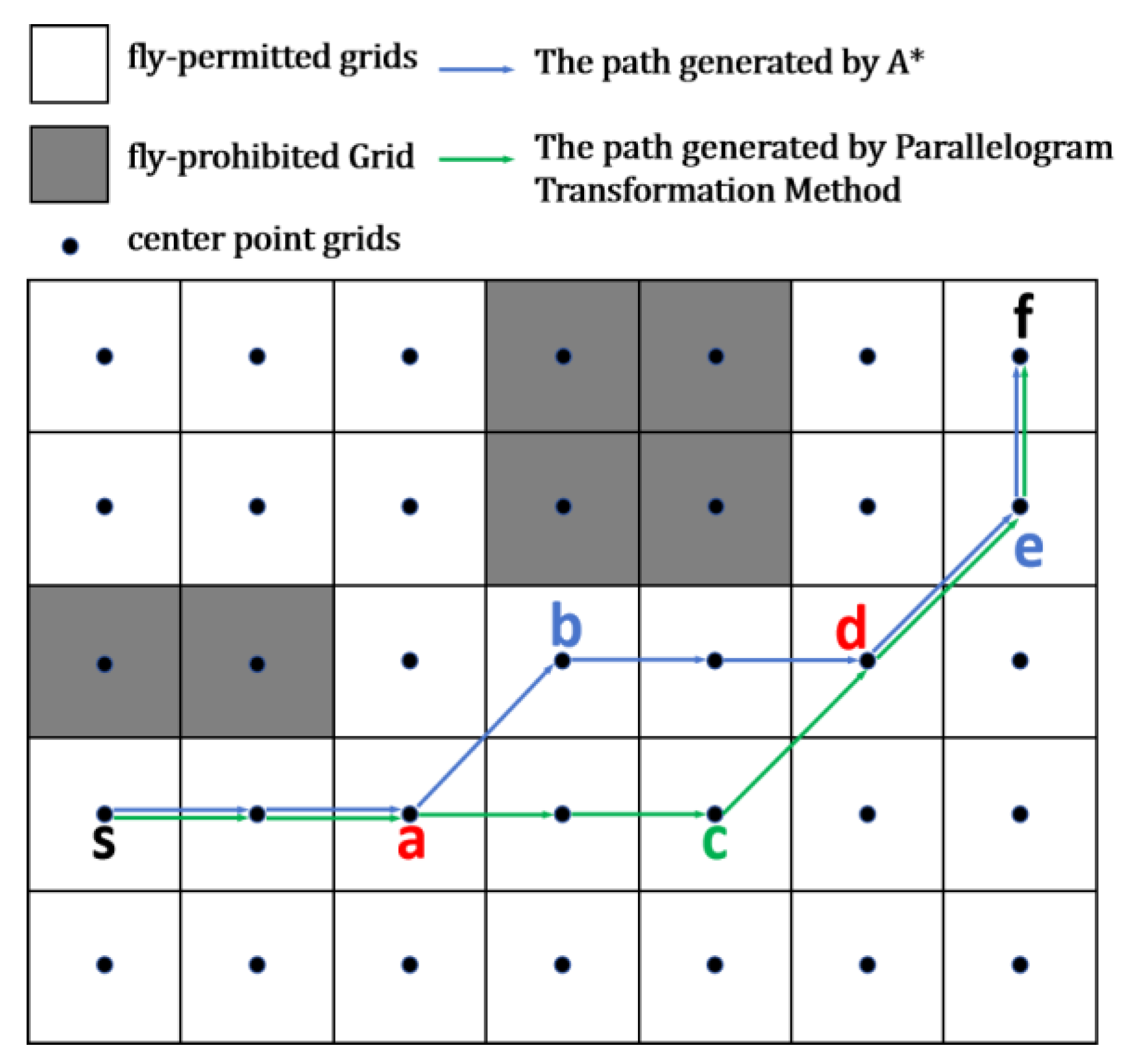
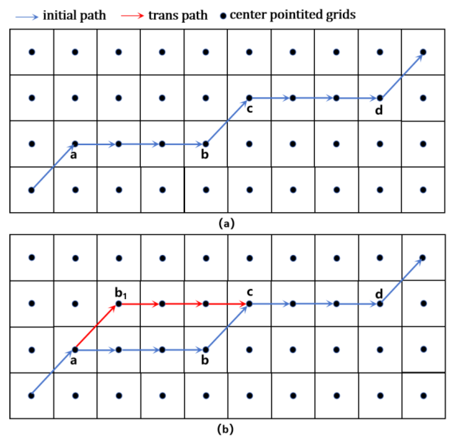
4.2.2. Parallelogram-Based Turning Point Optimization

Since the A* algorithm [36] is constrained by grid resolution and directional limitations, it relies on $h\left(t\right)$ Euclidean distance to search for and determine an optimal path. As shown in Figure 4, due to the proximity between $\mathrm{b}$ and $\mathrm{f}$ adjacent grids, the UAV will perform turning maneuvers at points $\mathrm{a}$ and $\mathrm{b}$, leading to an excessive number of turns in the planned route. To address this issue, this study considers the risk variation during UAV route segment translation and applies a parallelogram transformation method to optimize the initially planned turning points, thereby reducing unnecessary turns in the trajectory.

As shown in Figure 5a, the flight segment can be identified $\mathrm{a}\mathrm{b}//\mathrm{c}\mathrm{d}$, indicating that the segment $\mathrm{a}\mathrm{b}$ is eligible for parallelogram transformation. When either $\mathrm{a}\mathrm{b}$ or $\mathrm{b}\mathrm{c}$ satisfies

$$\mathrm{a}\mathrm{b}//\mathrm{c}\mathrm{d} \mathrm{a}\mathrm{n}\mathrm{d} \left(\mathrm{l}\mathrm{e}\mathrm{n}\right(\mathrm{a}\mathrm{b})\le l_{max} \mathrm{o}\mathrm{r} \mathrm{l}\mathrm{e}\mathrm{n}(\mathrm{b}\mathrm{c})\le l_{max})$$

(36)

where $l_{max}$ represents the maximum allowable translation distance for segment shifting; $\mathrm{l}\mathrm{e}\mathrm{n}\left(\mathrm{a}\mathrm{b}\right)$ denotes the Euclidean distance between turning points $\mathrm{a}$ and $\mathrm{b}$. When the above conditions hold, a parallel translation is applied to segment $\mathrm{a}\mathrm{b}$ and $\mathrm{b}\mathrm{c}$, as illustrated in Figure 5b.

The steps parallelogram-based turning point optimization considering risk cost are as follows:

Step 1: Compute the initially planned flight segment set $segment\_path\_ini=\{s_1,s_2,\dots ,s_n\}$, where $s_n$ belongs to the planned route. Establish a new flight segment set $segment\_path\_new=\left\{\right\}$, and move to Step 2.

Step 2: Determine the number of segments in $segment\_path\_ini$. If the number of segments is greater than 3, proceed to Step 3. Otherwise, add the segment from $segment\_path\_ini$ to $segment\_path\_new$ and move to Step 7.

Step 3: Identify the first set of consecutive segments $\mathrm{a}\mathrm{b},\mathrm{b}\mathrm{c}$ and $\mathrm{c}\mathrm{d}$ in $segment\_path\_ini$. If the segments satisfy Equation (36), proceed to Step 4; otherwise, move to Step 5.

Step 4: Extract the grid point set $s{et}_{ini}$ corresponding to the initial segments $\mathrm{a}\mathrm{b}$ and $\mathrm{b}\mathrm{c}$, and apply a parallel transformation ${\mathrm{a}\mathrm{b}}_1$ and ${\mathrm{b}}_1\mathrm{c}$ to their respective grid points $s{et}_{trans}$. Compute the risk cost for the $s{et}_{ini}$ and $s{et}_{trans}$ using the formula

$${Risk}_{seg}={\displaystyle \frac{\sum _{\rho =1}^M{E}_{\rho }}{M}}$$

(37)

where $M$ represents the total number of grid points in the path segment. If grid $\rho$ is classified as a restricted no-fly zone, then ${Risk}_{seg}=+\infty$. Using Equation (37), compute the risk values for both the original ${Risk}_{seg\_ini}$ and transformed segments ${Risk}_{seg\_trans}$, then move to Step 5.

Step 5: If ${Risk}_{seg\_ini}\ge {Risk}_{seg\_trans}$, apply the parallelogram transformation and add the ${ab}_1$ transformed segment to $segment\_path\_new$, move to Step 2. Otherwise, move to Step 6.

Step 6: Add $\mathrm{a}\mathrm{b}$ to the $segment\_path\_new$ and remove $\mathrm{a}\mathrm{b}$ from $segment\_path\_ini$, then repeat Step 2.

Step 7: End the transformation process.

The detailed algorithm flowchart is illustrated in Figure 6.

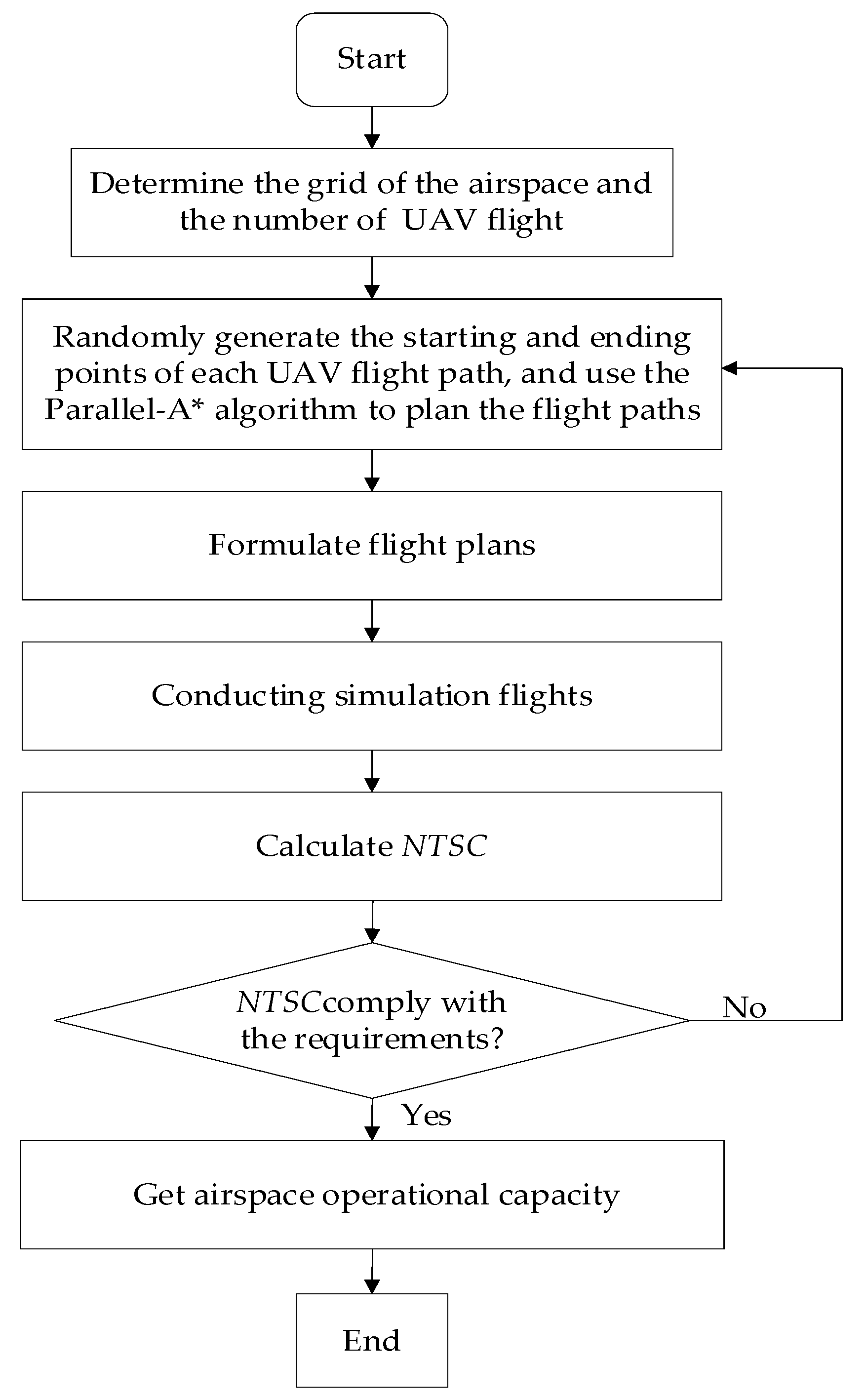
5. Airspace Capacity Assessment Method

This section conducts a modeling and analysis of urban low-altitude airspace operational capacity under free airspace conditions. The study utilizes the Parallel-A* algorithm to generate random UAV flight paths, providing a basis for capacity evaluation.

5.1. Airspace Operational Capacity Assessment Model

This study employs the Normalized Time Spent in Conflict ($NTSC$) [23] metric to quantify the acceptable level of airspace conflicts, with the UAV count corresponding to an acceptable $NTSC$ value defined as the airspace capacity. $NTSC$ is defined as the cumulative ratio of conflict duration to total flight time across all UAVs operating within the airspace, expressed as

$$NTSC={\displaystyle \frac{1}{K}}\sum _{i=1}^n{\displaystyle \frac{t_i^c}{t_i}}$$

(38)

where $K$ represents the total number of UAV flights; $t_i$ denotes the total flight duration of the $i$-th UAV; $t_i^c$ represents the total conflict time during which the $i$-th UAV encounters grid conflicts with other UAVs at the same moment. The grid conflict time refers to the duration required for a UAV to travel from the grid boundary to the grid center during its flight.

5.2. Conflict Simulation Model

The conflict simulation model operates within a predefined airspace grid and randomly generates non-repetitive UAV flight origin–destination pairs based on the number of simulated UAV flights per scenario. The Parallel-A* algorithm is employed to generate UAV flight paths. This study evaluates hourly airspace operational capacity by assigning a uniform take-off time for each UAV, formulating flight plans, and conducting simulation flights. Finally, calculate $\mathrm{N}\mathrm{T}\mathrm{S}\mathrm{C}$ and adjust the number of drone simulation flights based on $\mathrm{N}\mathrm{T}\mathrm{S}\mathrm{C}$ to obtain the final airspace operational capacity. The specific process is shown in Figure 7.

6. Experimental Analysis

6.1. Parameter Configuration

All the simulation experiments in this paper were conducted on a workstation equipped with an Intel(R)core(TM)i7-11800H CPU (This equipment manufacturer is Intel Corporation and it was sourced from Nanjing, China) and NVIDIA GeForce RTX 3060 Laptop(This equipment manufacturer is NVIDIA Corporation and it was sourced from Nanjing, China). For simulation analysis, this study selects geographic elevation data from Liuhe District, Nanjing. The designated airspace range is set as follows: Longitude is $118.77°\mathrm{E}-118.87°\mathrm{E}$, latitude is $32.29°\mathrm{N}-32.39°\mathrm{N}$, altitude is 15 m–205 m. Considering the spatial occupation in the airspace grid environment, the buildings and terrain features of Honglou District, Nanjing City are taken into account. The detailed parameters of the airspace grid environment are shown in

Table 4. Airspace grid environment and route planning model parameters.

Parameter	Value	Parameter	Value
$a_{max}/{\mathrm{m}/\mathrm{s}}^2$	6	$\beta /\mathrm{J}$	$100$
$L_{location}$/$\mathrm{m}$	4	$L_{uav}/\mathrm{d}\mathrm{B}$	110
$\rho$/$(\mathrm{k}\mathrm{g}/{\mathrm{m}}^3)$	1.225	$h_{uav}$/m	100
$C_d$	0.3	${\tau }_{max}$	3
$t_{trans}$	0.1	$d_{aircraft\_min}$/km	$0.5$
$P_{uav}$	${6.04\ast 10}^{-5}$	$d_{aircraft\_max}/\mathrm{k}\mathrm{m}$	$27.5$
$\alpha /J$	${10}^6$	${\delta }_{max}$	180

. The UAV of ARK-40 was selected for simulation analysis (the parameters of the unmanned aerial vehicle are shown in

Table 5. UAV parameters.

Model	Wingspan/m	${\mathbf{V}}_{\mathbf{m}\mathbf{a}\mathbf{x}}$/ $(\mathbf{m}/\mathbf{s})$	${\mathbf{m}}_{\mathbf{a}\mathbf{l}\mathbf{l}}$/ $\mathbf{k}\mathbf{g}$	${\mathbf{S}}_{\mathbf{o}}/\mathbf{m}$	${\mathbf{S}}_{\mathbf{v}}/\mathbf{m}$	${\mathbf{S}}_{\mathbf{h}}/\mathbf{m}$	$\mathbf{Number} \mathbf{of} \mathbf{Horizontal} \mathbf{Grids}$	Maximum Wind Resistance Level/Grade
$\mathrm{ARK}-40$	$2.36\times 1.2\times 0.6$	$14$	$46$	45.82	64	8.43	$173\times 173$	$7$

). During the simulation process, all the parameters of the unmanned aerial vehicle were the same, and the meteorological conditions factors such as wind force and visibility parameters all met the flight requirements of the ARK-40. Table 5 also lists the $S_v$ and $S_h$ of ARK-40. To facilitate subsequent experiments, the $S_h$ is set to 10 m.

6.2. Risk Analysis

6.2.1. Basic Information Distribution Maps

This section presents the basic information distribution maps, covering the spatial distribution of physical obstacles, sheltering factor, and population density. The visualization results are illustrated in Figure 8. Furthermore, the variation of the physical obstacles with the altitude layer is presented, as shown in Figure 9. This data represents the ratio of the number of grid cells occupied by physical obstacles at each $h_q$ layer to the total number of grid cells at that layer. Figure 8a shows the 3D geographic base map of Liuhe District, constructed using high-resolution remote sensing imagery. Figure 8b presents the physical obstacle distribution model, which quantitatively represents the spatial topology of buildings, transmission towers, and other 3D structures. Figure 9 indicates a significant negative correlation between obstacle density and altitude. When the flight altitude reaches a critical threshold of 115 m, no physical obstacles exist within the airspace. This threshold provides a key reference for airspace safety planning. Figure 8c illustrates the occlusion distribution map, composed of the sheltering factor defined in Table 3. Figure 8d displays the population density distribution map. The combined analysis of occlusion distribution and population density serves as an important foundation for modeling ground impact risk and third-party risk.

6.2.2. Environmental Risk Maps

This study employs a stratified sampling method to segment the $15–205\mathrm{m}$ airspace into $10 \mathrm{m}$ vertical layers, enabling a detailed analysis of environmental risk distribution across different altitude levels. Figure 10 illustrates the spatial characteristics of environmental risk distribution at various altitude $h_q=15 \mathrm{m},55 \mathrm{m},95 \mathrm{m},135 \mathrm{m}$ layers. Regarding the weights assigned to the risks of mid-air collision, ground impact, and third-party risk, this paper takes into account that ground impact will cause casualties. In line with the principle of prioritizing life, the weight of ground impact risk will be higher than that of mid-air collision risk and third-party risk, that is, $w_1=0.25$, $w_2=0.5$,${ w}_3=0.25$ [17]. Data analysis reveals that the highest risk levels are observed at $h_q=15 \mathrm{m}$ altitude layers, exhibiting a strong positive correlation with the spatial distribution of physical obstacles. As flight altitude increases, obstacle density decreases exponentially. When flight altitude reaches a certain threshold $h_q=135 \mathrm{m}$, the system monitoring results indicate that all architectural obstacles disappear, leading to a shift in risk composition. At higher altitudes, mid-air collision risk is significantly reduced, and ground impact risk, caused by UAV system failures, along with noise-related third-party risk, become the dominant risk factors. The environmental risk gradient curve in Figure 11 further quantifies this trend: risk values decrease with increasing flight altitude. When $h_q>115 \mathrm{m}$ the risk index stabilizes around the 0.15 threshold; airspace above 115 m exhibits low environmental risk, making it an optimal altitude range for UAV operations. This is also consistent with the current policies on UAVs in China [14] (where the airspace below 120 m is suitable for UAV flights), the United States [37] (where commercial UAVs are usually restricted to a height of 400 feet ≈ 122 m), and the European Union [38] (where open categories are limited to a height of 150 m (C₀)).

6.3. Path Planning Analysis

6.3.1. Parameter Analysis

In order to demonstrate the influence of different types of risk cost on the Parallel-A* algorithm, we conducted four sets of path planning simulation analyses at the level of $h_q=105 \mathrm{m}$. The specific designs of these four analyses are as follows: (1) Path 1: Without considering any risks, it degenerates into the A* algorithm; (2) Path 2: Considering only the risk of ground impact, that is, $w_1=0$, $w_2=1$,${ w}_3=0$; (3) Path 3: Considering only the risk of ground impact, that is, $w_1=0.5$, $w_2=0.5$,${ w}_3=0$; (4) Path 4: Taking into account all three types of risks, that is, $w_1=0.25$, $w_2=0.5$,${ w}_3=0.25$. In the four path scenarios, except for Path 1, since the risk of ground impact involves personal safety and property loss, the simulation analysis of different parameters for the remaining paths also involves the risk of ground impact. The parameter settings for Path 2 are mainly oriented towards suburban scenes in open areas. The parameter settings for Path 3 mainly consider commercial areas without considering risks such as noise from third parties. The parameter settings for Path 4 mainly consider residential areas. Four sets of simulation analyses conducted 100 random path planning experiments, respectively, obtaining the average comprehensive risk ${\overline{R}}_{path}$ along the route and the average number of turning points ${\overline{T}}_{path}$. The results are shown in

Table 6. The simulation analysis results of four sets of path planning. In this table, “↓” represents the growth percentage rate, while “↑” represents the decline percentage rate.

	Computational Results		Performance Ratio Compared with Path 1
	${\overline{R}}_{path}$	${\overline{T}}_{path}$	${\overline{R}}_{path}$	${\overline{T}}_{path}$
Path 1	2.42	3.51	100%	0%
Path 2	1.51	7.66	38%↓	118%↑
Path 3	1.32	8.53	45%↓	143%↑
Path 4	1.20	9.60	50%↓	173%↑

. The specific formulas are as follows:

$${\overline{R}}_{path}={\displaystyle \frac{\sum _{p=1}^N{R}_{path}^p}{N}}$$

(39)

$${\overline{T}}_{path}={\displaystyle \frac{\sum _{p=1}^N{T}_{path}^p}{N}}$$

(40)

where $N$ represents the total number of path planning iterations; $R_{path}^p$ and $T_{path}^p$ denote the comprehensive risk value and number of turning points for the $p$-th planned route, respectively, which can be expressed as

$$R_{path}^p=\sum _{i=1}^{len\left(path\right)}{R}_i$$

(41)

$$R_{path}^p=\sum _{i=1}^{len\left(path\right)-2}angle[i,i+1,i+2]$$

(42)

where $len\left(path\right)$ represents the total number of grid points in the planned path $p$, and $\mathrm{a}\mathrm{n}\mathrm{g}\mathrm{l}\mathrm{e}[i,i+1,i+2]$ denotes the angle formed between adjacent grid points $\mathrm{\angle }\mathrm{a}\mathrm{b}\mathrm{c}$, $(i,i+1)$ and $(i+1,i+2)$, while when $\mathrm{\angle }i,i+1,i+2=180°$, $\mathrm{a}\mathrm{n}\mathrm{g}\mathrm{l}\mathrm{e}[i,i+1,i+2]=0$, and $\mathrm{\angle }i,i+1,i+2<180°$, $\mathrm{a}\mathrm{n}\mathrm{g}\mathrm{l}\mathrm{e}[i,i+1,i+2]=1$.

From Table 6, it can be seen that Path 1 has a relatively high ${\overline{R}}_{path}$; due to the consideration of the risk of ground impact, when conducting the Path 2 path planning experiment, the densely populated areas were avoided, and its ${\overline{R}}_{path}$ decreased by 38%; when the risk of air collision was added, the Path 3 simulation experiment also avoided the densely populated solid obstacle areas, and its ${\overline{R}}_{path}$ decreased by 45%; Path 4 considered all three types of risks, and compared with Path 3, the ${\overline{R}}_{path}$ of Path 4 was further reduced by 5%. In addition, it can also be seen that as the number of risk types increases, the complexity of risks within the airspace environment further increases, and the value of ${\overline{T}}_{path}$ gradually rises. This is due to the avoidance of high-risk areas during path planning. This experiment verified the optimization effect of integrating multiple risk types on path safety.

6.3.2. Algorithm Comparison

The Parallel-A* algorithm proposed in this study exhibits multi-dimensional optimization characteristics in path planning, enabling it to avoid obstacles, high-risk areas, and reduce the number of turning points. This paper also compares the A* algorithm and the Weight-A* algorithm as the control group and conducts experimental analysis with $h_q=105 \mathrm{m}$. The schematic diagram of the path planning result is shown in Figure 12. As can be seen from Figure 12, the A* algorithm, due to its sole consideration of the Euclidean distance cost, has the potential safety hazard of crossing high-risk airspace in its planned path; although the Weight-A* algorithm improves the safety of the path through the risk-avoidance strategy, it has a large number of turning points; the Parallel-A* algorithm constructed in this paper has fewer turning points than the Weight-A* algorithm and avoids high-risk areas.

This paper also conducted 100 independent random experiments for A*, Weight-A*, and Parallel-A*, respectively, under the condition of $h_q=105 \mathrm{m}$, as shown in

Table 7. Analysis of comprehensive risk and number of turning points in path planning of A*, Weight-A*, and Parallel-A*.

Algorithm	Comprehensive Risk (Mean ± SD)	Number of Turning Points (Mean ± SD)
Weight-A*	$1.66\pm 1.27$	$15.11\pm 7.23$
Parallel-A*	$1.20\pm 0.92$	$9.6\pm 4.52$
A*	$2.42\pm 3.00$	$3.51\pm 1.37$
ANOVA Results (F-value/p-value)	$F=9.67$ $p=8.49\times {10}^{-5}<0.05$	$F=133.95$ $p=3.43\times {10}^{-5}<0.05$

. Based on the ANOVA method, the significance test was conducted on the comprehensive risks and the number of turning points of the three algorithms. The results showed that there were extremely significant differences in both sets of indicators (comprehensive risk: $F=9.67$, ${p=8.49\times 10}^{-5}$; number of inflection points: $F=133.95$, ${p=3.43\times 10}^{-5}$). Specifically, the Parallel-A* algorithm ($1.20\pm 0.92$) outperforms all others in terms of the comprehensive risk. Its comprehensive risk is significantly lower than that of the Weight-A* ($1.66\pm 1.27)$ algorithm and the A* ($2.42\pm 3.00$) algorithm. In terms of the number of turning points, the number of turning points of the Parallel-A* algorithm ($9.6\pm 4.52$) is lower than that of the Weight-A* algorithm ($15.11\pm 7.23)$. In summary, this experiment demonstrates that the Parallel-A* algorithm can significantly reduce the number of path turning points while lowering the comprehensive risk, verifying its superiority over traditional algorithms.

Figure 13 and Figure 14 illustrate the trends in average comprehensive risk and the number of turning points for the A*, Weight-A*, and Parallel-A* algorithms at varying altitude levels. From Figure 13, it is evident that as altitude increases, the average comprehensive risk of all three algorithms gradually decreases. Notably, at all altitude levels, the Parallel-A* algorithm maintains the lowest average comprehensive risk, demonstrating superior safety performance. From Figure 14, the A* algorithm consistently exhibits the lowest number of turning points throughout the experiment. This is because the A* algorithm does not consider risk factors in path planning, resulting in fewer turns along the trajectory. Among the risk-aware algorithms, Parallel-A* and Weight-A*, the proposed Parallel-A* algorithm consistently produces fewer turning points than the Weight-A* algorithm, indicating a more efficient path structure. In conclusion, the analysis of ${\overline{R}}_{path}$ and ${\overline{T}}_{path}$ confirms that the proposed Parallel-A* algorithm achieves fewer turning points and lower comprehensive risk, demonstrating high safety and operational efficiency in UAV path planning.

6.4. Analysis of Low-Altitude Airspace Operational Capacity

As can be seen from Section 6.3, the Parallel-A* algorithm designed in this paper has low risks and few inflection points. Therefore, based on the Parallel-A* algorithm, this paper also generates UAV flight paths with low comprehensive risks for conducting airspace operation capacity assessment. Due to the fact that UAV flight involves different operational scenarios and the differentiated management requirements of low-altitude flight management service departments, the $\mathrm{N}\mathrm{T}\mathrm{S}\mathrm{C}$ threshold can be dynamically adjusted according to specific needs. Therefore, this paper provides an analysis of airspace operation capacity under different thresholds. Figure 15 analyzes the situation of the airspace operation capacity varying with $h_q\in [45 \mathrm{m},205 \mathrm{m}]$ under different conflict thresholds ($\mathrm{N}\mathrm{T}\mathrm{S}\mathrm{C}=0.05,0.01,0.015,0.020,0.025,0.03$). To facilitate a better analysis, Figure 15 also presents the variation of $R_i$ with $h_q$. As can be seen from Figure 15, at the same $h_q$, the increase of $\mathrm{N}\mathrm{T}\mathrm{S}\mathrm{C}$ will further enhance the capacity of spatial operation. Furthermore, as $h_q$ increases, the spatial operation capacity of the same spatial domain under $\mathrm{N}\mathrm{T}\mathrm{S}\mathrm{C}$ will increase accordingly and become stable. When the number of physical obstacles in the spatial domain is zero (that is, when $h_q$ is around 115 m), the spatial capacity will tend to stabilize. It can also be observed that the trend of airspace operation capacity and $R_i$ is opposite. The smaller $R_i$ is, the greater the airspace operation capacity will be. This phenomenon indicates that the airspace operation capacity will increase as the overall risk of airspace decreases.

7. Conclusions

This study develops a digital low-altitude airspace grid-based model tailored for urban risk environments, focusing on UAV path planning and operational capacity assessment. By constructing management-scale and operation-scale grids of vertical and horizontal partitioning, integrating multi-source data such as urban 3D geographic information, population density, and parameters of UAV, a risk discretization quantitative assessment model was established. The risks of mid-air collision, ground impact, third-party risk, and turning risk of unmanned aerial vehicles were systematically analyzed. To enhance the flight efficiency of UAVs and reduce risks, a method for optimizing a parallelogram-based turning point optimization path planning method considering both risks and transportation costs was proposed. The Parallel-A* algorithm was established to solve the path. Furthermore, an airspace operational capacity assessment model and a conflict simulation model are established based on the Parallel-A* algorithm, providing a theoretical foundation for airspace capacity estimation in urban low-altitude airspace under risk conditions.

Using Liuhe District, Nanjing as the experimental area, this study analyzes the impact of buildings, sheltering factor, and population density on UAV operations and validates the effectiveness of the proposed method through simulation experiments. The results indicate that as altitude increases, the comprehensive risk gradually decreases and stabilizes. In the four sets of path planning analyses under different risk parameters, the path planned by comprehensively considering the three types of risks has the smallest comprehensive risk, which verifies the optimization effect of integrating multiple risk types on path safety. In the comparative experiments of different path planning methods, the algorithm proposed in this paper outperforms the traditional A* and Weight-A* algorithms in terms of average comprehensive risk and the number of turning points. This fully demonstrates the advantages of the Parallel-A* algorithm in risk avoidance and efficiency improvement. Meanwhile, the research has found that the operational capacity of low-altitude airspace in cities increases as the comprehensive risk decreases, and stabilizes after the comprehensive risk is reduced.

This research provides a scientific basis for the rational utilization and management of urban low-altitude airspace, facilitating the optimization and sustainable allocation of airspace resources. Furthermore, it lays a solid foundation for the large-scale deployment and safe operation of UAV applications in urban environments, offering significant theoretical contributions and practical value. Future research will extend to three-dimensional path planning and divide the urban environment into regions. Dynamic risk environment parameters will be set according to the specific environmental requirements of each region to meet the demands of three-dimensional obstacle avoidance and dynamic height optimization in complex urban environments.

References

1. Wu, K.; Lan, J.; Lu, S.; Wu, C.; Liu, B.; Lu, Z. Integrative Path Planning for Multi-Rotor Logistics UAVs Considering UAV Dynamics, Energy Efficiency, and Obstacle Avoidance. Drones 2025, 9, 93. [Google Scholar] [CrossRef]
2. Farrag, T.A.; Askr, H.; Elhosseini, M.A.; Hassanien, A.E.; Farag, M.A. Intelligent Parcel Delivery Scheduling Using Truck-Drones to Cut down Time and Cost. Drones 2024, 8, 477. [Google Scholar] [CrossRef]
3. Zhang, H.; Wang, F.; Feng, D.; Du, S.; Zhong, G.; Deng, C.; Zhou, J. A Logistics UAV Parcel-Receiving Station and Public Air-Route Planning Method Based on Bi-Layer Optimization. Appl. Sci. 2023, 13, 1842. [Google Scholar] [CrossRef]
4. Callewaert, N.; Pareyn, I.; Acke, T.; Desplinter, B.; Van de Pitte, K.; Van Vooren, J.; De Meyer, M.; Seeldraeyers, E.; Peeters, F.; De Meyer, S.F.; et al. Limited Impact of Drone Transport of Blood on Platelet Activation. Drones 2024, 8, 752. [Google Scholar] [CrossRef]
5. Tang, P.; Li, J.; Sun, H. A Review of Electric UAV Visual Detection and Navigation Technologies for Emergency Rescue Missions. Sustainability 2024, 16, 2105. [Google Scholar] [CrossRef]
6. Zhou, Y.; Jin, Z.; Shi, H.; Shi, L.; Lu, N.; Dong, M. Enhanced Emergency Communication Services for Post-Disaster Rescue: Multi-IRS Assisted Air-Ground Integrated Data Collection. IEEE T Netw. Sci. Eng. 2024, 11, 4651–4664. [Google Scholar] [CrossRef]
7. Tan, Y.; Yi, W.; Chen, P.; Zou, Y. An adaptive crack inspection method for building surface based on BIM, UAV and edge computing. Autom. Constr. 2024, 157, 105161. [Google Scholar] [CrossRef]
8. Aela, P.; Chi, H.; Fares, A.; Zayed, T.; Kim, M. UAV-based studies in railway infrastructure monitoring. Autom. Constr. 2024, 167, 105714. [Google Scholar] [CrossRef]
9. Mohamed Salleh, M.F.B.; Wanchao, C.; Wang, Z.; Huang, S.; Tan, D.Y.; Huang, T.; Low, K.H. Preliminary concept of adaptive urban airspace management for unmanned aircraft operations. In Proceedings of the 2018 AIAA Information Systems-AIAA Infotech@ Aerospace, Kissimmee, FL, USA, 8–12 January 2018; p. 2260. [Google Scholar]
10. Xu, X.Y.; Wan, L.J.; Chen, P.; Dai, J.B.; Cai, M. An Airspace Raster Representation Method Based on GeoSOT Grid. J. Air Force Eng. Univ. (Nat. Sci. Ed.) 2021, 22, 15–22. [Google Scholar]
11. Tang, X.M.; Gu, J.W.; Zheng, P.C.; Li, T. A Method for Unmanned Aerial Vehicle (UAV) Dynamic Geographic Fence Planning Based on Spatial Gridization. China Patent 202010909173.0A, 2020. [Google Scholar]
12. Shi, H.F.; Wang, Z.Y.; Zheng, Y.; Xu, Y.B. Refined Management System of Airspace Resources Based on BeiDou Grid Location Code. J. Civ. Aviat. 2022, 6, 44–47. [Google Scholar]
13. Martin, T.; Huang, Z.F.; McFadyen, A. Airspace risk management for UAVs a framework for optimising detector performance standards and airspace traffic using JARUS SORA. In Proceedings of the 2018 IEEE/AIAA 37th Digital Avionics Systems Conference (DASC), London, UK, 23–27 September 2018; pp. 1516–1525. [Google Scholar]
14. CAAC Management Regulations for Trial Operation of Specific Types of UAVs. Available online: https://www.caac.gov.cn/XXGK/XXGK/GFXWJ/201902/t20190201_194511.html (accessed on 1 February 2019).
15. Shao, P. Risk assessment for UAS logistic delivery under UAS traffic management environment. Aerospace 2020, 7, 140. [Google Scholar] [CrossRef]
16. Banerjee, P.; Gorospe, G.; Ancel, E. 3D representation of UAV-obstacle collision risk under off-nominal conditions. In Proceedings of the IEEE Conference on Aerospace, Big Sky, MT, USA, 6–13 March 2021; pp. 1–7. [Google Scholar]
17. Pang, B.; Hu, X.; Dai, W.; Low, K.H. UAV path optimization with an integrated cost assessment model considering third-party risks in metropolitan environments. Reliab. Eng. Syst. Safe 2022, 222, 108399. [Google Scholar] [CrossRef]
18. Primatesta, S.; Rizzo, A.; la Cour-Harbo, A. Ground Risk Map for Unmanned Aircraft in Urban Environments. J. Intell. Robot. Syst. 2020, 97, 489–509. [Google Scholar] [CrossRef]
19. Harrelson, A.V.G.C. Computing the Shortest Path: A* Search Meets Graph Theory. Proc. Soda 2005, 2005. [Google Scholar] [CrossRef]
20. Zhang, H.H.; Zhang, L.D.; Liu, H.; Gang, H. Track Planning Model for Logistics Unmanned Aerial Vehicle in Urban Low-altitude Airspace. J. Transp. Syst. Eng. Inf. Technol. 2022, 22, 256–264. [Google Scholar]
21. Jung, D.; Tsiotras, P. On-line path generation for unmanned aerial vehicles using B-spline path templates. J. Guid. Control Dyn. 2013, 36, 1642–1653. [Google Scholar] [CrossRef]
22. Damilano, L.; Guglieri, G.; Quagliotti, F.; Sale, I.; Lunghi, A. Ground control station embedded mission planning for UAS. J. Intell. Robot. Syst. 2013, 69, 241–256. [Google Scholar] [CrossRef]
23. Bulusu, V.; Sengupta, R.; Liu, Z. Unmanned aviation: To be free or not to be free? In Proceedings of the 7th International Conference on Research in Air Transportation, Philadelphia, PA, USA, 20–24 June 2016. [Google Scholar]
24. Starita, S.; Strauss, A.K.; Fei, X.; Jovanović, R.; Ivanov, N.; Pavlović, G.; Fichert, F. Air traffic control capacity planning under demand and capacity provision uncertainty. Transp. Sci. 2020, 54, 882–896. [Google Scholar] [CrossRef]
25. Cho, J.; Yoon, Y. How to assess the capacity of urban airspace: A topological approach using keep-in and keep-out geofence. Transp. Res. Part C Emerg. Technol. 2018, 92, 137–149. [Google Scholar] [CrossRef]
26. Vascik, P.D.; Hansman, R.J. Development of vertiport capacity envelopes and analysis of their sensitivity to topological and operational factors. In Proceedings of the AIAA Scitech 2019 Forum, San Diego, CA, USA, 7–11 January 2019; p. 526. [Google Scholar]
27. Zhou, J.; Jin, L.; Wang, X.; Sun, D. Resilient uav traffic congestion control using fluid queuing models. IEEE T Intell. Transp. 2020, 22, 7561–7572. [Google Scholar] [CrossRef]
28. Wang, Y.L.; Zhang, S.; Wu, Y.J. Path Planning Algorithm Based on Improved A* Smoothness. Comput. Appl. Softw. 2025, 42, 258–263. [Google Scholar]
29. Bulusu, V.; Polishchuk, V.; Sengupta, R.; Sedov, L. Capacity estimation for low altitude airspace. In Proceedings of the 17th AIAA Aviation Technology, Integration, and Operations Conference, Denver, CO, USA, 5–9 June 2017; p. 4266. [Google Scholar]
30. Jin, A.; Cheng, C.Q. Spatial Data Coding Method Based on Global Subdivision Grid. J. Geomat. Sci. Technol. 2013, 30, 284–287. [Google Scholar]
31. Interim Regulation on the Administration of the Flight of Unmanned Aircraft; The State Council of the People’s Republic of China, Central Military Commission of the People’s Republic of China: Beijing, China, 2024.
32. Park, S.; Lee, M.C.; Kim, J. Trajectory Planning with Collision Avoidance for Redundant Robots Using Jacobian and Artificial Potential Field-based Real-time Inverse Kinematics. Int. J. Control Autom. Syst. 2020, 18, 2095–2107. [Google Scholar] [CrossRef]
33. Xinhui, R.; Caixia, C. Construction and application of third-party risk model for unmanned aerial vehicle operation in urban environment. China Saf. Sci. J. 2021, 31, 15–20. [Google Scholar]
34. Zhou, R.J. Research on UAV Path Planning. Master’s Thesis, University of Electronic Science and Technology of China, Chengdu, China, 2023. [Google Scholar]
35. Zhang, Q.Q.; Xu, W.W.; Zhang, H.H.; Zou, Y.Y.; Chen, Y.T. Path planning for logistics UAV in complex low-altitude airspace. J. Beijing Univ. Aeronaut. Astronaut. 2020, 46, 1275–1286. [Google Scholar]
36. Baganoff, F.K.; Maeda, Y.; Morris, M.; Bautz, M.W.; Townsley, A.L.K. Chandra X-Ray Spectroscopic Imaging of Sgr A* and the Central Parsec of the Galaxy. 2001. Available online: https://ui.adsabs.harvard.edu/abs/2003ApJ...591..891B/exportcitation (accessed on 8 February 2001).
37. Beard, R.W.; McLain, T.W. Small Unmanned Aircraft: Theory and Practice; Princeton University Press: Princeton, NJ, USA, 2012. [Google Scholar]
38. Huttunen, M. The u-space concept. Air Space Law 2019, 44, 69–89. [Google Scholar] [CrossRef]
Figure 1. Vertical–horizontal grid partitioning schematic.
Drones 09 00320 g001
Figure 2. Schematic of operation-scale grid.
Drones 09 00320 g002
Figure 3. Quantification of the risk of mid-air collisions.
Drones 09 00320 g003
Figure 4. Parallel-A* algorithm example. In this figure, “s-a-b-d-f” represents the path planning by A* algorithm, and “s-a-c-d-f” represents the path planning by the Parallel-A* algorithm.
Drones 09 00320 g004
Figure 5. Schematic of the parallelogram transformation method. In this figure, “a-b-c-d” represents the initial pathby A* algorithm, and “a-b1-c-d” represents the trans path by the Parallel-A* algorithm.
Drones 09 00320 g005
Figure 6. Algorithm flowchart of parallelogram-based turning point optimization path planning method.
Drones 09 00320 g006
Figure 7. Conflict simulation process.
Drones 09 00320 g007
Figure 8. Basic information distribution maps.
Drones 09 00320 g008
Figure 9. Proportion of physical obstacles by altitude.
Drones 09 00320 g009
Figure 10. Environmental risk distribution maps at different altitudes. The red part in the picture indicates the prohibited entry area of the grid.
Drones 09 00320 g010
Figure 11. Environmental risk gradient curve.
Drones 09 00320 g011
Figure 12. Path planning result diagrams of A*, Weight-A*, and Parallel-A* algorithms. The red part in the picture indicates the prohibited entry area of the grid.
Drones 09 00320 g012
Figure 13. Variation of average comprehensive risk with altitude.
Drones 09 00320 g013
Figure 14. Variation of average number of turning points with altitude.
Drones 09 00320 g014
Figure 15. Variation of airspace capacity and with altitude.
Drones 09 00320 g015