A Numerical Analysis of the Temporal and Spatial Temperature Development during the Ultrasonic Spot Welding of Fibre-Reinforced Thermoplastics

Abstract

The ultrasonic spot welding of fibre-reinforced thermoplastic laminates has received great interest from researchers, mainly in the fields of aerospace and automotive industries. It offers an efficient solution to join large thermoplastic composite parts through the spot welding approach with a high level of automation. In this paper, the temporal and spatial development of the temperature in an ultrasonic weld spot between two fibre-reinforced thermoplastic laminates was modelled. During the ultrasonic welding of thermoplastic composite laminates without energy directors a sudden temperature jump in the weld spot is usually observed. The temperature increase occurs rapidly up to the decomposition of the thermoplastic matrix and causes the degradation of the weld spot. To understand the temperature distribution within the weld spot and to calculate its temporal development, the thermal problem was analysed using a two-dimensional explicit finite difference method. To evaluate the models, the calculated time traces of the temperature in the weld spot were compared with the experimentally obtained values under comparable conditions.

1. Introduction

In the ultrasonic welding of polymers, mechanical vibrations with a frequency usually between 20 kHz and 45 kHz are applied through an ultrasonic sonotrode, accompanied with a static pressure, perpendicular on the outer surface of one of the mating parts to be joined. The vibrations cause internal heating due to intensive intermolecular and surface friction at and around the joint interface [1]. The joint heats up locally and rapidly until the polymers melt/soften. Then, the vibration excitation is interrupted and the polymers solidify under a static pressure applied by the sonotrode. In order to focus the ultrasonic vibration energy at a desired interfacial region, protrusions (usually triangular, or rectangular) are introduced at those locations in practical applications [2,3]. Due to the geometry and material of the protrusions, also called energy directors (ED), these have a stiffness less than the stiffness of the preceding layers, therefore the majority of the applied strain energy focuses at the ED, and thus heat up, soften/melt and flow preferably. When welding fibre-reinforced thermoplastic (FRTP) laminates without energy directors, there is insufficient polymer at the weld zone. The lack of the matrix could result in excessive heating of the weld spot and thus the quality of the weld might be reduced [4,5,6,7]. Even though the ultrasonic spot welding without energy directors requires additional process control, the demands for the preparation of the welding zone and the weldments are simplified significantly [4,6].

A configuration for the ultrasonic spot welding without energy directors was discussed and modelled by the authors in [8]. The configuration, which was called the differential ultrasonic spot welding (DUS), is illustrated schematically in Figure 1. The focusing mechanism of the vibration energy was explained by two interrelated phases: at the initial phase, the cyclic deformations caused an intensive temperature increase due to frictional heating at the interface between the laminates. The second phase started as soon as the weld interface softened/melted, then the frictional heating diminished, and a concentrated viscoelastic heating dominated the process. An approach to avoid the overheating of the matrix for this spot welding configuration was discussed by the authors in [4,6]; the weld power time derivative was used to detect the overheating initiation of the weld spot and it was avoided by the controlled reduction of the vibration amplitude.

One way to monitor weld spot development during ultrasonic welding is the measurement of the temperature through placement of thermocouples or temperature measurement films in the weld spot [5,7,9,10]. However, introducing thermocouples on one hand might slightly influence the initial phase of the welding process and on the other hand it gives limited information on a single spot in the weld zone. The presence of the thermocouple might induce a strain concentration around it. This can cause a higher heating rate in the initial phase of the welding compared to welding without thermocouples. However, as soon as the weld interface softens, the influence of the thermocouple can be neglected.

In order to analyse the temperature development and the cause of the overheating in the weld spot, the thermal problem was investigated by means of numerical modelling. It would be computationally not reasonable to model the entire 2–3 s duration of the 30 kHz ultrasonic welding process with a 3D finite element method (FEM) with explicit or implicit time integration and capture the viscoelastic and friction heat generation at each cycle. If solved using these methods, then the model would require a very large number of sub-steps to cover the entire weld duration. This problem has been solved by Levy et al. [11,12,13] through the implementation of the time-homogenisation method. The space-time homogenisation has been implemented by Boutin et al. [14] to study the heat generation by mechanical work in structures subjected to a cyclic loading for long durations of time, such as in fatigue testing. Wang et al. [15] used a coupled thermal-mechanical quasi-static finite element model to investigate the heating and bonding mechanisms during the ultrasonic welding of carbon fibre-reinforced polyether ether ketone (PEEK) through triangular ED. The cycle-jump method was used by Cojocaru and Karlsson [16] to accelerate the FEM analysis of the failure of the structures subjected to cyclic loading. Jedrasiak et al. [17] implemented sequentially coupled deformation and thermal models to simulate the ultrasonic welding of dissimilar metallic alloys. The deformation model calculated the heat generation over a short period of time and the thermal model predicted the thermal field over a longer period of time. This approach has made the model computationally efficient. The cycle jump method eliminates the need to simulate each cycle of the loading, although it averages the amount of heat that is predicted to be generated during the ultrasonic vibration dissipation by a very short amount of time. The short period of time might include several cycles or a few hundred cycles of vibration.

One of the main challenges facing the realistic modelling of the heat generation during ultrasonic welding process was the lack of an exact method for determining the loss modulus of the polymeric matrix $E_m^{″}\left(T\right)$ as a function of temperature at the desired ultrasonic welding frequency range. Some of the known methods to measure $E_m^{″}\left(T\right)$ are the dynamic mechanical analysis (DMA) and the through transmission ultrasonic testing. The known commercially available DMA is a standardised method that can be used to measure $E_m^{″}\left(T\right)$ up to a frequency of 100 Hz. The ultrasonic method can be implemented to calculate the $E_m^{″}\left(T\right)$ from the time-of-flight and attenuation of the ultrasonic waves through the material at frequencies ranging between a few hundred kHz and a few MHz [18]. Levy et al. [11] measured $E_m^{″}\left(T\right)$ of the pure polyetherimide (PEI) polymer from room temperature up to a temperature of 235 °C at five frequency values in the range of 0.1 Hz and 100 Hz. By implementing a time-temperature superposition, the curves have been extrapolated to the ultrasonic welding frequency of 20 kHz. Zhang et al. [19] measured the relaxation modulus curves at various temperatures for polymethylmethacrylate (PMMA) and used the data to calculate the dynamic loss modulus as a function of time. Another promising approach is the inverse determination of material properties using experimental measurements and computational simulation, such as the methods proposed by Jedrasiak et al. [17] and Willis et al. [20].

In the present study, an explicit finite difference method (eFDM) with cycle jumps was implemented to determine the temperature development and distribution in the ultrasonic weld spot between a pair of carbon fibre-reinforced thermoplastic (CFRTP) laminates throughout the entire duration of a DUS process [21]. The inverse measurement method was applied to determine the loss modulus $E_m^{″}\left(T\right)$ of the polymeric matrix at the ultrasonic welding frequency range by minimizing the difference between the experimental data and the predictions from implemented numerical model in which the loss modulus was the adjustable parameter. This approach was preferred for two reasons: first, the flexibility that it provided to investigate various physical phenomena, hypotheses and theories of the DUS process; and second, to establish a numerical basis for the improvement of the active control system of the ultrasonic welding, which was presented in [6]. The numerical simulation served to explain the energy direction mechanism during DUS, clarify the causes of the overheating, detect the overheating initiation regions, and thus confirm the findings made in [8].

2. Materials and Methods

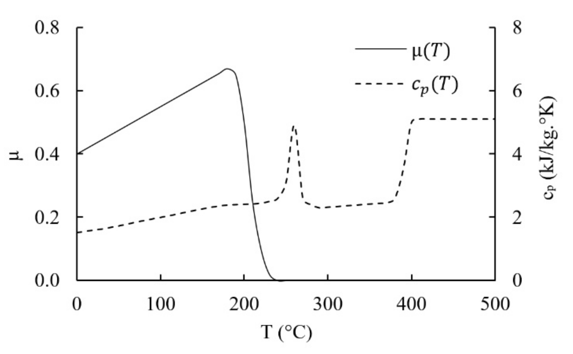
2.1. Modelling of the Heat Sources

The mechanisms governing the heating of the material during the ultrasonic welding are studied in detail by several researchers [11,12,13,19,22]. It may be summed up by two major heat generation mechanisms. The heating in the initial phase is dominated by the interface frictional heating. It can be simplified as the heat dissipation due to Coulomb damping [8,11]. The amount of friction heat ${\dot{q}}_{fric}$ generated per unit time at a unit of surface area is given in Equation (1), where $\omega$ is the angular ultrasonic frequency, $\mu$ the friction coefficient at the weld interface, $u_0$ the relative slippage at the interface [11,19], ${\sigma }_0$ is the total interfacial pressure in the transverse direction, and $\alpha$ is the coefficient for the hammering effect [23].

$${\dot{q}}_{fric}={\alpha }^2\frac{\omega \mu u_0{\sigma }_0}{\pi }$$

(1)

After the polymer at the interface heats up to the melting temperature (or glass transition temperature for amorphous polymers), the friction gradually disappears and the heat generation by the viscoelastic heating (also called intermolecular frictional heating) dominates. The viscoelastic heating is taken from literature as the dissipated strain energy by viscoelastic damping [11,12,13,19,22]. This heat is a volumetric quantity and is related to the dynamic loss modulus $E^{″}\left(T\right)$ of the viscoelastic material. The amount of heat ${\dot{q}}_{vis}$ generated by viscoelastic damping per unit time and per unit volume can be expressed by Equation (2), where ${\epsilon }_0$ is the amplitude of the cyclic strain.

$${\dot{q}}_{vis}={\alpha }^2\frac{\omega E^{″}{\epsilon }_0^2}{2}$$

(2)

It was assumed in the present study that the heat was mainly generated by the polymeric matrix. Considering the loss modulus of polymer and carbon fibre materials, the dissipated strain energy by the fibres was much smaller than the dissipation of polymers and thus was neglected. If Equation (2) was used to predict the heat generation by viscoelastic strain energy dissipation mechanisms, the calculated heat would have been underestimated compared to real welding processes. Based on the Reuss composite model [24,25], the laminate was considered as subsequent layers of matrix and fibre. When FRTP laminates are subjected to compression in the transverse thickness direction 33 the strain in each layer can be expressed by Equation (3). Assuming that ${\epsilon }_{33}$ was the transverse total strain in the composite, $E_c^{*}\left(T\right)$ was the complex modulus of the composite, the fibre and matrix volume fractions were equal $v_f=v_m=0.5$ and the Poisson’s ratio mismatch was ignored.

$${\epsilon }_{m0}.E_m^{*}\left(T\right)={\epsilon }_{f0}.E_{f,33}={\epsilon }_{33}.E_{c,33}^{*}\left(T\right)$$

(3)

In a CFRTP, the transverse elastic modulus of the fibres is much greater than the complex modulus of the polymeric matrix $E_{f,33}\gg E_m^{*}$, consequently the strain component in the matrix becomes much greater than the strain component of the fibre ${\epsilon }_m\gg {\epsilon }_f$. Therefore, the Equation (2) should be modified and the strain component in the matrix ${\epsilon }_{m0}$ and the matrix loss modulus $E_m^{″}\left(T\right)$ should be used instead, which results in the following Equation (4) for viscoelastic volumetric heating of the matrix ${\dot{q}}_m$.

$${\dot{q}}_m={\alpha }^2\frac{\omega E_m^{″}{\epsilon }_{m0}^2}{2}$$

(4)

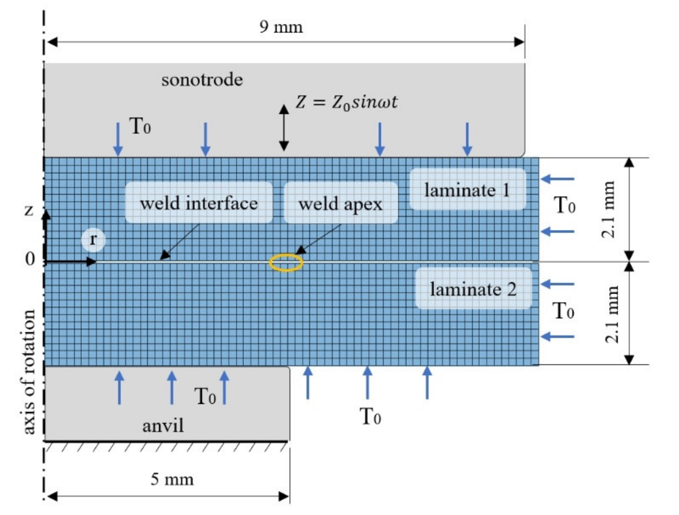
2.2. The Numerical Model

The heat generation and transfer were simulated using the eFDM in the numerical computing environment (MATLAB R2015b, Natick, MA, USA). The method used in the present study divided the weld duration into finite time increments $\delta t$. It was considered that the material properties were temperature-dependent, and they were known at the beginning of each time increment for each element based on the temperature calculated in the previous time step for that element. The generated heat due to surface friction Equation (1) and viscoelastic energy dissipation Equation (4) of the ultrasonic vibration was averaged over the time increment $\delta t$. Similarly, the heat transfer inside the volume and the heat transferred to the environment were averaged over this time increment. As a result, the temperature increase $\delta t$ at the end of each increment $\delta t$ was calculated in each element and added to the temperature $T\left(t+\delta t\right)=T\left(t\right)+\delta T$. The new temperature value was used to update the related composite properties by using interpolations of a corresponding lookup table. The time increment $\delta t=4 \mathrm{ms}$ was determined to be appropriate by means of a convergence analysis. To model the heat generation and the heat transfer, rotational symmetry was used to simplify the weld spot geometry as 2D-axysimmetric approximation and to reduce its degrees of freedom. This assumption of symmetry was valid because it was agreed by several researchers [11,12,15], which analysed the woven fabric laminates and approximated these laminates as transverse isotropic material (i.e., having equal properties in the in-plane direction and different in the out-of-plane direction).

The physical system of interest was the DUS welding of a CFRTP laminate pair (compare Figure 1 and Figure 2). The laminate type selected for the simulation models and the experimental analysis was a 2 × 2 twill woven carbon fabric reinforced polyamide (PA) 6.6. The theoretical fibre volume fraction was $v_f=50\%$. The laminates had a thickness of $h_1=h_2=2.1 \mathrm{mm}$, they were fixed in position and supported at the bottom side by means of a flat-end anvil, which had a circular contact with the lower laminate (Figure 2). The diameter of the anvil end was $D_a=10 \mathrm{mm}$ and the diameter of the sonotrode end was $D_h=18 \mathrm{mm}$. The sonotrode applied a cyclic sinusoidal longitudinal displacement $Z\left(t\right)=Z_0\sin \left(\omega t\right)$ perpendicular to the upper laminate with a frequency of $f=\omega /2\pi =30 \mathrm{kHz}$. Only, the weld zone bound inside the radius of the sonotrode was taken into consideration for the numerical analysis. The cross sections of the laminates were discretised by central node square elements with an element edge length of $\Delta r=\Delta z=0.15 \mathrm{mm}$. This resulted in a number of $m=14$ rows of elements for each laminate. For each row, a number of $n=68$ elements were used for the calculation (see Figure 2). The stacking direction of the transverse isotropic laminate was $33 \left(or zz\right)$. It was assumed that the 33 direction matched the $z$-axis of the cylindrical coordinate system and the planar direction 11 matched the radial direction $r$. Each element contained the properties of the averaged composite material based on the classical lamination theory (CLT), such as described in [26,27].

The block diagram of the calculations in a time increment is given in Figure 3. The vibration amplitude $Z_0$, static weld force $F_w$ and vibration frequency ω were used as input variables. The hammering effect coefficient $\alpha$ has a strong correlation with both the $Z_0$, $F_w$ and it has a significant influence of the heating rate [12,23]. The hammering effect coefficient was considered constant for a given value of $F_w$. The amount of slip and the interfacial pressure at each element were imported from the separately solved explicit dynamic 3D FEM analysis of the deformations, which was discussed in [8]. The amplitude distributions of the slippage $u_0$ and the interfacial pressure ${\sigma }_0$ were considered as constants for the initial stage of the process for a given value of $Z_0$. However, it was assumed that as soon as the interfaces heated up above 230 °C, the influence of the slippage diminished. The distributions of the $u_0$ and ${\sigma }_0$ along the radial direction in the weld interface for $Z_0=28 \mathsf{\mu }\mathrm{m}$ are plotted in Figure 4.

The material properties such as the transverse composite storage moduli $E_{c,33}^{\prime }\left(T\right),$ the matrix storage modulus $E_m^{\prime }\left(T\right)$, the matrix loss modulus $E_m^{″}\left(T\right)$, the friction coefficient $\mu \left(T\right)$ and the specific heat capacity of the composite $c_p\left(T\right)$ were input as functions of temperature (see Figure 5). The direction dependant thermal conduction coefficients of the composite $k_1, k_2, k_3$, and $k_h$ as well as the density of the composite ${\rho }_{comp}$ were approximated as constants for the predicted temperature range (

Table 1. Relevant thermal and mechanical properties (at room temperature) of the theoretical laminate based on a 2 × 2 twill woven carbon fabric reinforced Polyamide 6.6.

Property	Value
${\rho }_{comp}$ (density of the composite)	1515 kg/m3
$E_{c,11}^{\prime }, E_{c,22}^{\prime }$ (in-plane elasticity modulus of the composite)	55 GPa
$E_{c,33}^{\prime }$ (transverse elasticity modulus of the composite)	11.5 GPa
Tg (glass transition temperature)	53 °C
Tmi (melting point)	240 °C
Tm (melting point)	260 °C
Tdi (thermal decomposition initiation)	358 °C [35]
Td (thermal decomposition temperature)	400 °C [35]
k1, k2 (in-plane thermal conductivity)	2.6 W/(m K)
k3 (transverse thermal conductivity)	0.6 W/(m K)
$k_h$ (convective heat transfer coefficient)	1.5 W/(m2 K)

). These material properties were defined to match the real experimental laminates based on values provided by the material supplier and some values taken from literature [28,29,30,31,32,33] under the assumption of laminate transverse isotropy. However, as already stated by several researchers [13,19,22], there was no direct reliable method to measure the elastic and loss moduli against a temperature range for the given ultrasonic frequency of $f=30 \mathrm{kHz}$. Thus, in the following section, a method is discussed that allowed estimating the loss modulus from experimentally measured process curves that have a strong correlation with the temperature-dependent loss modulus.

From the available data in [29,31,34], a curve for the $\mathsf{\mu }\left(T\right)$ as a function of temperature was assumed in the present study (Figure 5). At room temperature, the friction coefficient was μ(27 °C) = 0.4 and it was assumed that $\mathsf{\mu }\left(T\right)$ increased linearly up to a temperature of $T=$ 200 °C. At this elevated temperature, the surfaces started to stick to each other and the slippage gradually decreased. Due to initiation of melting at a temperature point of $T=$ 230 °C and the frictional heating was eliminated. This phenomenon was modelled by assuming a coefficient of μ(T > 230 °C) = 0 in the friction heat generation equation (1). The heat capacity $c_p\left(T\right)$, the glass transition temperature $T_g$, the melting initiation temperature $T_{mi}$ and the melting point $T_m$ were determined through the differential scanning calorimetry (DSC). A heating rate of 20 °C/min and starting temperature of $T=$ 23 °C were used. The $c_p\left(T\right)$ values were measured from the room temperature and up to 300 °C (Figure 5). It was assumed that the heat capacity should abruptly increase as soon as the temperature of the matrix reached the decomposition initiation temperature $T_{di}=$ 358 °C. The anvil, the sonotrode, and the environment were assumed to have an infinite heat capacity and a constant temperature of $T_0=$ 27 °C (compare Figure 2). The remaining properties of these CFRTP laminates were taken from Table 1.

The in-plane elasticity modulus of the composite was determined by static tension testing. The tests were carried out according to the International Organization for Standardization ISO 527-1 and the specimens were prepared according to ISO 527-4 (type-3 specimens). The transverse elasticity modulus was determined using the ultrasonic through transmission approach [17]. In which an ultrasonic frequency of 5 MHz was used. These initial values at room temperature were used for the calculations in the 3D FEM. For the eFDM analysis, the temperature dependant mechanical properties were calculated using the rule of mixtures. From the measured composite moduli at room temperature, the initial fibre moduli were determined. Considering the fibre moduli as constant in the given temperature range of interest, the temperature dependant composite moduli were calculated based on the rule of mixtures. The remaining data were provided by the material supplier.

In Figure 6B, the components of the heat energy per unit time for an element located in the weld interface are illustrated. The elements had sizes of $\Delta r=\Delta z=0.15 \mathrm{mm}$ and an angle increment of $\theta =$ 1°. Each element had the interfacial surface area $\Delta S_z$, an element volume $\Delta V$ and a matrix volume $\Delta V_m=\Delta V{v}_m$ (Figure 6). The volume and the surface of the elements increased with increasing radial location $r$. Thus, each element based on its location and temperature was subjected to a surface heat due to friction ${\dot{Q}}_{fric}$ and it generated an internal volumetric heat due to viscoelastic dissipation ${\dot{Q}}_m$. These were given by Equations (5) and (6) respectively:

$${\dot{Q}}_{fric}\left(r,z,T\right)={\dot{q}}_{fric}\left(r,z,T\right). \Delta S_z\left(r,z\right)$$

(5)

$${\dot{Q}}_m\left(r,z,T\right)={\dot{q}}_m\left(r,z,T\right). \Delta V_m\left(r,z\right)$$

(6)

The heat conduction equation in general for a finite element subjected to an external heat flux and an internal generated heat for the cylindrical coordinate system was defined by the following Equation (7), as described by [36,37]:

$$\frac{1}{\mathrm{r}}\frac{\partial }{\partial r}\left[k_{r}r\frac{\partial T}{\partial r}\right]+\frac{1}{r^2}\frac{\partial }{\partial \theta }\left[k_{\theta }\frac{\partial T}{\partial \theta }\right]+\frac{\partial }{\partial z}\left[k_z\frac{\partial T}{\partial z}\right]+\frac{{\dot{Q}}_m}{\Delta V}+\frac{{\dot{Q}}_{fric}}{\Delta V}=\rho c_p\frac{\partial T}{\partial t}$$

(7)

For the investigated problem of heating during the ultrasonic welding of composite laminates, it was assumed that the amount of heat produced at each radial location was equal. Therefore, there was no temperature difference between the neighbouring elements located at the same radius, and thus the heat transfer in the angular direction $\phi$ was negligible due to the rotational symmetry. This yields the differential form of the balance of energy which is given in Equation (8):

$$\frac{k_r}{r}\left[\frac{\partial T}{\partial r}+r\frac{{\partial }^{2}T}{\partial r^2}\right]+k_z\frac{{\partial }^{2}T}{\partial z^2}+\frac{{\dot{Q}}_m}{\Delta V}+\frac{{\dot{Q}}_{fric}}{\Delta V}=\rho c_p\frac{\partial T}{\partial t}$$

(8)

Moreover, for elements that were not located at the interface, the friction heat flux was not present. Thus, the heat equation was rewritten as in Equation (9).

$$\frac{k_r}{r}\left[\frac{\partial T}{\partial r}+r\frac{{\partial }^{2}T}{\partial r^2}\right]+k_z\frac{{\partial }^{2}T}{\partial z^2}+\frac{{\dot{Q}}_m}{\Delta V}=\rho c_p\frac{\partial T}{\partial t}$$

(9)

The elements exchange heat with the neighbouring elements in the $z$-direction and in the radial $x$-direction. It was expressed by Equations (10), (11), and (12) using a central difference quotient for the approximation of the spatial derivatives.

$$k_z\frac{{\partial }^{2}T}{\partial z^2}=k_3\left(\frac{T_{i+1,j}-2T_{ij}+T_{i-1,j}}{\Delta z^2}\right)$$

(10)

$$k_r\frac{{\partial }^{2}T}{\partial r^2}=k_1\left(\frac{T_{i,j+1}-2T_{ij}+T_{i,j-1}}{\Delta r^2}\right)$$

(11)

$$\frac{k_r}{r}\frac{\partial T}{\partial r}=\frac{k_1}{r}\left(\frac{T_{i,j+1}-2T_{ij}+T_{i,j-1}}{\Delta r}\right)$$

(12)

In order to predict the viscoelastic heating, the strain in each element was calculated at each time step, The stiffness of each element $K{\left(T\right)}_{ij}$ was calculated from Equation (13) based on the temperature-dependent complex modulus of the composite $E_c^{*}{\left(T\right)}_{ij}$, assuming that the normal of the element surface area $\Delta S_z^{ij}$ was parallel to the $z$-direction and that the height $\Delta z$ was constant. From $K{\left(T\right)}_{ij},$ the total stiffness of each layer $i$ at each time step was calculated from Equation (14), considering that only the elements within the weld apex were being compressed. This in turn was used to calculate the displacement amplitude in each row of elements $Z_i$, with the assumption that the total amplitude of deformation (vibration displacement amplitude) $Z_0$ was constant throughout the process duration. The stain amplitude of the element ${\epsilon }_{m0, ij}$ was predicted using Equations (15)–(17) under the assumption that the matrix volume fraction was uniform throughout the elements. The strain amplitude (the strain component in the $zz$ direction) in the matrix of each element was calculated by Equation (18).

$$K{\left(T\right)}_{ij}=E_c^{*}{\left(T\right)}_{ij}.\frac{\Delta S_z^{ij}}{\Delta r}$$

(13)

$$K_l^i\left(T\right)={\displaystyle \sum _{j=1}^{n_{in}}}{K}_{ij}\left(T\right)$$

(14)

$$\frac{1}{K\left(T\right)}={\displaystyle \sum _{i=1}^m}\frac{1}{K_l^i\left(T\right)}$$

(15)

$$Z_i.K_l^i\left(T\right)=Z_0.K\left(T\right)$$

(16)

$${\epsilon }_{ij}=\frac{Z_i}{\delta r}$$

(17)

$${\epsilon }_{m0}^{ij}.E_m^{*}\left(T\right)={\epsilon }_{ij}.E_c^{*}\left(T\right)$$

(18)

2.3. Experimental Setup

2.3.1. The Laminates

The laminate type selected for the simulation models and the experimental analysis was a 2 × 2 twill woven carbon fabric (T-700 carbon fibre with 12 K filaments/roving) reinforced PA 6.6 (Evolite PA66 CF, Cytec Industrial Materials (Derby) Ltd, Heanor Derbyshire, UK). According to the material datasheet, the nominal fibre volume fraction was $v_f=50\%$ and the thickness of the laminate was $h=2.1\pm 0.1 \mathrm{mm}$. It was produced by a film-stacking process of 7 layers of 2 × 2 twill woven carbon fabric prepregs.

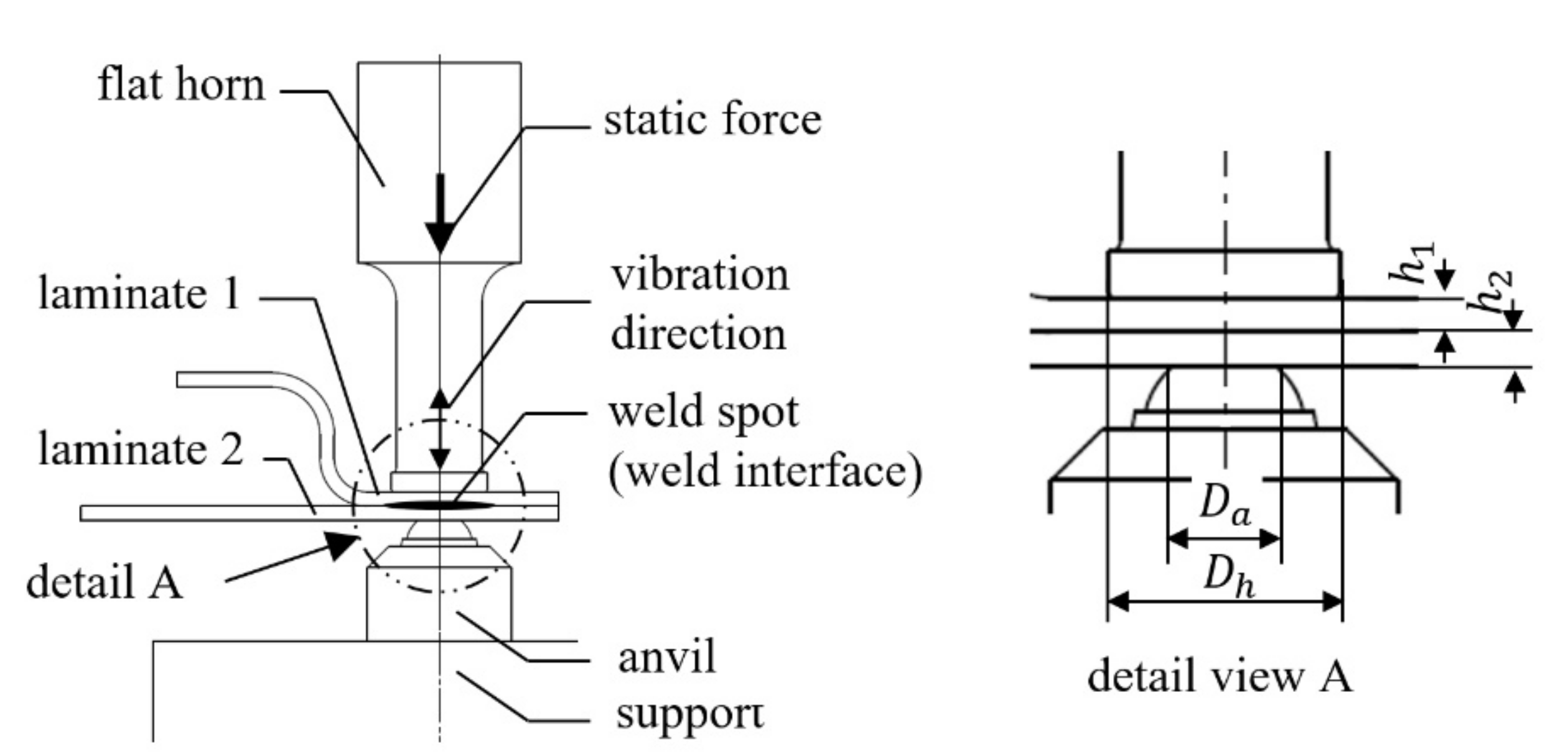
2.3.2. The Welding Apparatus

A commercial ultrasonic welder (TCS5 + MAG-W030024, TELSONIC AG, Bronschhofen, Switzerland) was used for the experimental studies. The generator was capable of outputting a nominal maximum power of 2400 W with a nominal frequency of $f=30 \mathrm{kHz}$. The ultrasonic stack consisted of a converter for a frequency of $f=30 \mathrm{kHz}$, a titanium booster with a horn gain of 5 and a steel catenoidal flat end steel horn with a horn gain of 4. According to the laser vibrometer measurements, the stack provided a maximum base to peak displacement amplitude of $Z_{max}=28 \mathsf{\mu }\mathrm{m}$ at the horn end. The ultrasonic stack was installed on a pneumatic press (Telsonic USP3000E, TELSONIC AG, Bronschhofen, Switzerland) which delivered a maximum compressing static force of $F_{max}=3000 \mathrm{N}$ on the workpieces. The horn end had a diameter of $D_h=18 \mathrm{mm}$ and the anvil had a diameter of $D_a=10 \mathrm{mm}$. This yielded a static pressure of 19.5 MPa between the two mating laminates. The anvil had its first natural frequency of about 42 kHz to avoid resonance vibrations in the rig at the operating frequency of $f=30 \mathrm{kHz}$.

2.3.3. Procedure

For the purpose of verifying the numerical model, several experiments were carried out to measure the temperature in the centre of the circular welding zone between the laminates during the ultrasonic welding process. The laminates were cut into stripes with dimensions of 48 × 98 mm. For hot-dry conditioning, the samples were placed in a convection oven maintained at an elevated temperature of 75 °C for 96 h. Afterwards, specimens were cooled down one by one to the ambient temperature and then they were used for the welding procedure. K-Type thermocouples with a wire diameter of 0.08 mm were carefully placed in the centre of one of the laminate pairs. The centre of the laminate was marked with the aid of a digital calliper. A notch was cut in the middle of the two long sides of the laminate stripe. The thermocouple was positioned in the marked centre and the wires were pulled sideways through the notches (see Figure 7B), where they were glued using a fast curing adhesive (Loctite 401, Henkel AG and Co. KGaA, Düsseldorf, Germany). The laminates were positioned on top of each other in a crosswise arrangement in a way that captured the thermocouple on their centre and on the centre axis of the ultrasonic stack using the fixture shown in Figure 7A. A 0.2 s pulse of ultrasonic vibration was applied through the horn on the top laminate to embed the thermocouple into the laminates. Using this approach, the positioning of the thermocouple was guaranteed and the effect of the strain concentration around the thermocouple was reduced. Computed tomography scans of the weld spots confirmed that the thermocouples remained unaffected after the welding process (compare [6]).

The temperature recording was undertaken using a universal amplifier and a data recorder with a sample rate of 300 Hz. A Butterworth digital filter was applied to remove the random noise of the measured signals. The temperature measurements were carried out with a vibration displacement amplitude $Z_0=23 \mathsf{\mu }\mathrm{m}$. The weld duration of $t_w=3 \mathrm{s}$ was adjusted to capture the complete heating phenomena. A number of 6 repetitions were carried out to collect statistical data for the development of temperature in the welding zone. The temperature measurement was undertaken for two static weld forces. The first set of welds (case-1) were carried out with $F_{w1}=450 \mathrm{N}$ and the second set (case-2) with $F_{w2}=650 \mathrm{N}$. The case-1 measurements were used for the loss modulus adjustment calculations and the case-2 measurements were used to validate the simulation results.

3. Results and Discussion

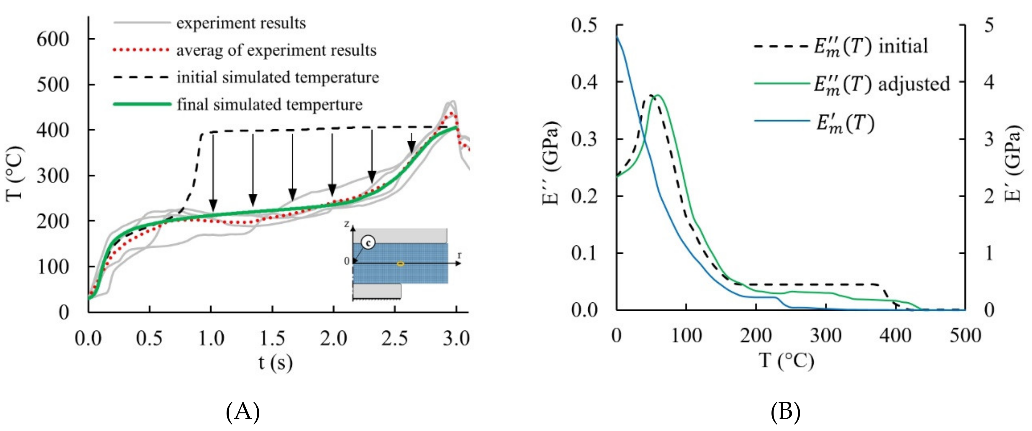
3.1. Calculation of the Matrix Loss Modulus

The adjustment of the $E_m^{″}\left(T\right)$ was carried out by an iterative optimisation algorithm. The initial $E_m^{″}\left(T\right)$ of the PA66 matrix and its $E_m^{\prime }\left(T\right)$ were extrapolated from the measured data given in [11,33,38,39]. The parameters for the simulated weld were comparable with the experimental case-1. The hammering effect for the simulated case-1 was chosen ${\alpha }^2=0.535$ as constant throughout the weld duration. These initial values of the loss and storage moduli resulted in inaccurate curves of the temperature in the weld centre (the broken black curve in Figure 8)) in comparison to the averaged measured temperature data illustrated as dotted red curve in Figure 8A. The initial simulated curve had a similar trend as the measured temperature. However, the second temperature increase occurred much earlier. The reason for this deviation between the calculated and the experimental curves was the inaccurate and overestimated $E_m^{″}\left(T\right)$ for the applied ultrasonic spot welding configuration.

The solver compared the changing rate of the calculated temperature and the measured temperature at each time step, if the measured rate was higher than the calculation then $E_m^{″}\left(T\right)$ was reduced (adjusted) and vice versa. The adjustment was done with a factor equivalent to the amount of difference between the measured and calculated rates of change. Since the temperature increase history would change by changing the $E_m^{″}\left(T\right)$, once an adjustment was done, the iteration started again from the beginning. The iterations continued until the temperature values resulting from the model were in good agreement with those from the real measurements of case-1 at each time increment. The final curve is plotted as the solid green line in Figure 8A. The adjusted and initial $E_m^{″}\left(T\right)$ curves are plotted as functions of temperature in Figure 8B. Comparing the initial curve and the adjusted curve of the loss modulus, the discrepancy between initial simulated temperature and the averaged measured temperature can be argued (compare Figure 8A,B).

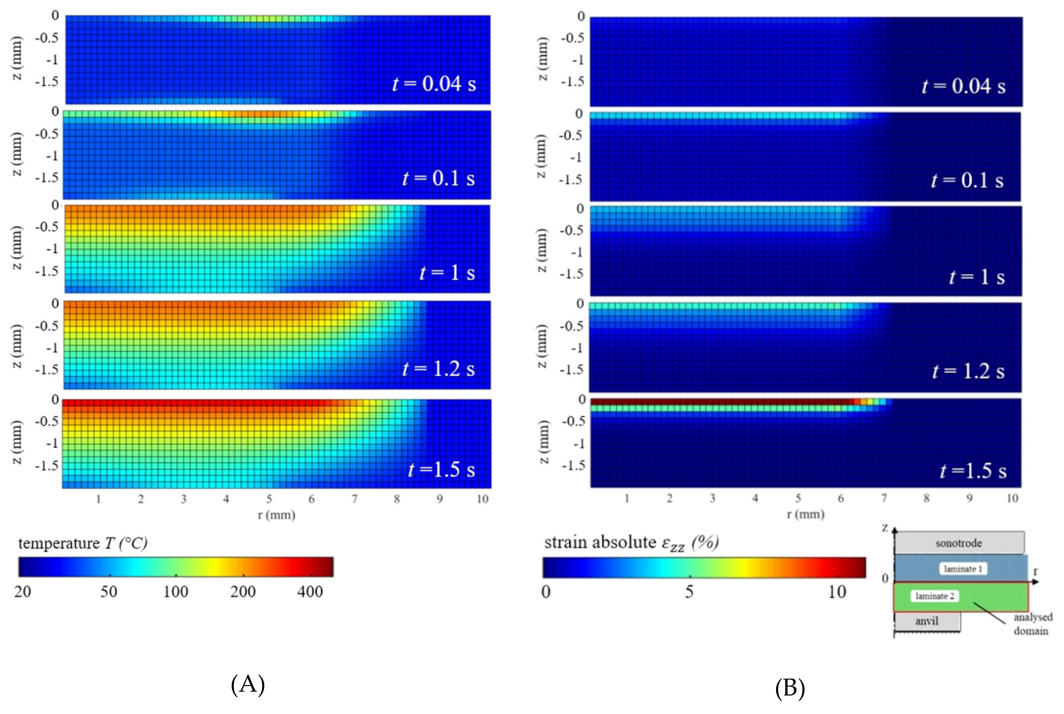
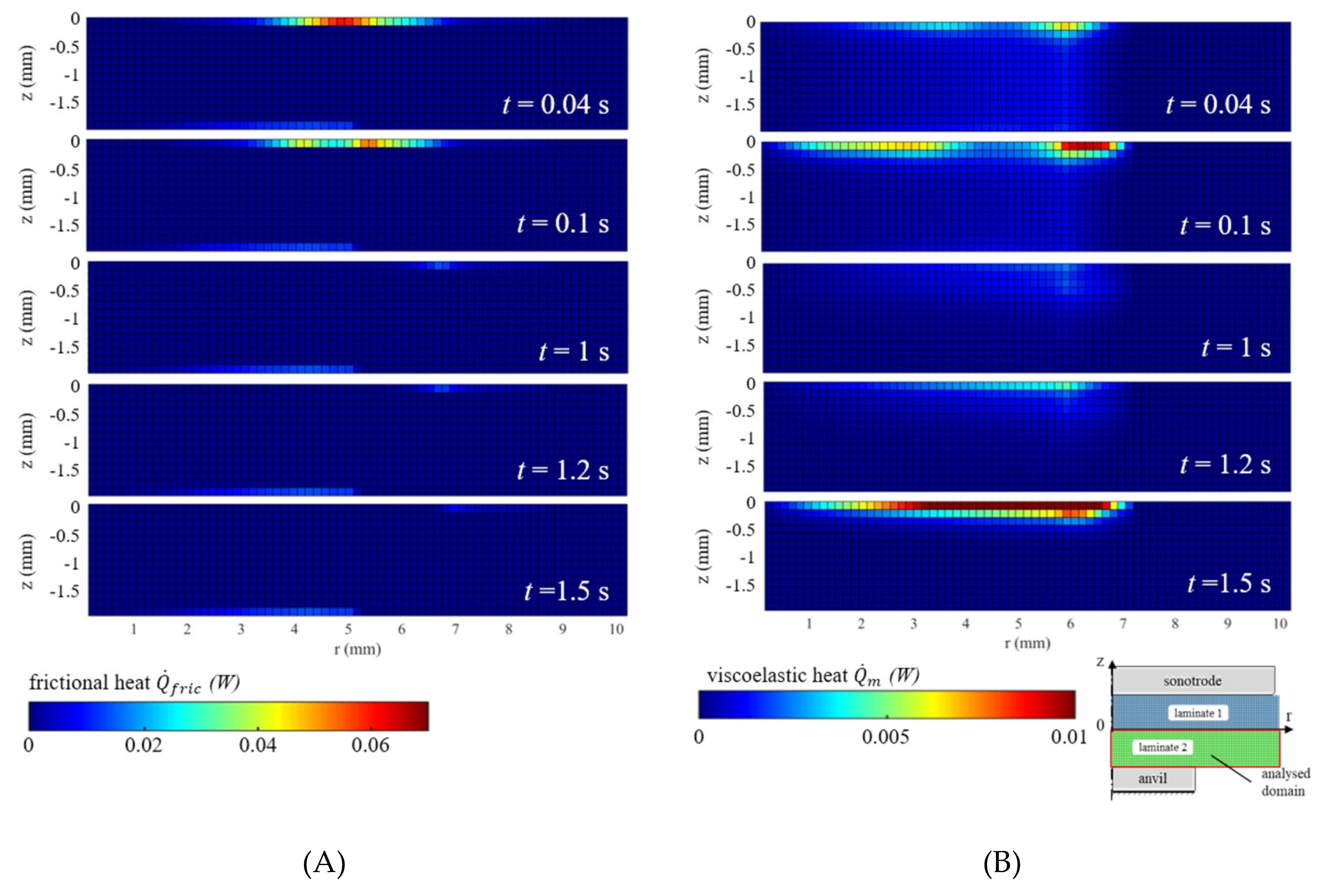
3.2. Analysis of the Thermal Problem

The temporal development of the temperature during a DUS process delivered significant information about the weld spot formation. The predicted temperature developed differently based on the spatial location within the modelled laminate. In order to validate the model, the weld parameters were set as in the experimental case-2, consequently ${\alpha }^2=0.6$ was chosen to compensate the increase of $F_w$. It can be seen in Figure 9 that the average temperature curve measured from the case-2 experiment showed a good agreement with the simulated counterpart in the weld centre (compare dotted red curve and solid curve in Figure 9A,B).

For the interfacial elements, a common trend for the temperature curves was observed (Figure 9A). The temperature rapidly increased in the initial phase, the increase rate $\frac{dT}{dt}=1780$ °C/s was calculated to be the highest at the weld apex ($a\left(r=5, \phi =0, z=0\right)$) and it gradually reduced when getting closer to the weld centre. At $t_s=1.25 \mathrm{s}$ and as soon as the temperature in the weld centre exceeded the matrix melting initiation temperature ($T_{mi}\approx$ 240 °C), an abrupt increase of the temperature with a rate of about $dT/dt=$ 650 °C/s for the entire interface was observed. This continued until the thermal decomposition temperature of the matrix was exceeded and only then was a thermal equilibrium achieved and the temperature curve stabilised. From the temperature temporal development at different positions in the thickness, it was observed that the temperature increase rate decreased as moving away from the weld interface (Figure 9B). A heating rate of $dT/dt=$ 1150 °C/s in the initial phase was observed at the interfacial element in the weld centre ($c\left(r=0, \phi =0, z=0\right)$). The temperature increase rate was much lower with a value of $dT/dt=$ 190 °C/s at the position of ($d\left(r=0, \phi =0, z=-0.6 \mathrm{mm}\right)$). The second abrupt temperature increase did not take place for the locations away from the weld interface. The elements halfway through the thickness ($e\left(r=0, \phi =0, z=-1.2 \mathrm{mm}\right)$) had an average heating rate of $dT/dt=$ 48 °C/s. the temperature at that position did not reach the melting temperature throughout the welding duration.

The temperature distribution in the laminates showed a slight correlation to the corresponding strain distribution (Figure 10A). Nevertheless, the strain distribution alone could not deliver sufficient information about the spatial heat generation (Figure 10B). Because the heat generation did not only depend on the strain distribution but also on the temperature dependant material properties (especially the loss and elastic moduli). Therefore, the spatial distribution of the heat generated by viscoelastic and frictional dissipations were observed on separate colour maps through the laminate thickness at five characteristic times (Figure 11). The analysed domain was the laminate 2, which was in contact with the anvil.

Directly after the application of the vibrations ($0 \mathrm{s}<t<0.05 \mathrm{s}$), the strain was almost uniform throughout the laminate thickness with a tendency towards strain concentration at the laminate contact with the anvil. Up to a weld time of $t\le 0.04 \mathrm{s}$, the heating was mostly dominated by the friction heating and it was most intensive around the weld apex ($3.5 \mathrm{mm}<r<6.5 \mathrm{mm}$) at the weld interface. The friction heat at the weld apex was almost eight times higher than the volumetric viscoelastic heat in the rest of the laminate volume. As soon as the temperature around the weld apex in the weld interface exceeded 200 °C, the friction coefficient became higher and the surfaces started to stick to one another. Consequently, the relative friction movement between the laminates and the resulting friction heating gradually diminished.

The local friction heating in the initial phase gave way for two interconnected phenomena to occur: it reduced the local stiffness (due to reduction of $E_m^{\prime }\left(T\right)$) of the interfacial layers between the laminates, and it heated up the composite around the weld apex through heat transfer to a temperature range at which the $E_m^{″}\left(T\right)$ was higher than at room temperature. These two phenomena led to the accelerated heating of the interface. Therefore, a high and focused viscoelastic energy dissipation occurred in the weld centre (Figure 11B) at time $t=0.1 \mathrm{s}$). However, at this specific moment, a gap in the viscoelastic heat at the weld apex was observed. This was due to the low $E_m^{″}\left(T\right)$ of the weld apex in comparison to that in the weld centre (compare Figure 8B).

In the following period (i.e., $0.3 \mathrm{s}<t<1 \mathrm{s}$), the heating was much slower in the entire interface, because the friction heating was almost completely eliminated and the interface temperature was in a range where the $E_m^{″}\left(T\right)$ was relatively small (see Figure 8B) for the loss modulus values). Although a moderate strain concentration around the interface was observed, but due to the low loss $E_m^{″}\left(T\right)$ values only a relatively small amount of heat was generated. This phase with a low heating rate was called the transition phase. During the transition phase, the remaining layers became softer and the strain distribution gradient in the interfaces became less sharp.

However, as soon as the entire interface inside the weld centre ($r\le 6 \mathrm{mm}$) reached the melting initiation temperature ($T_{mi}\approx$ 240 °C), a very sharp drop of the matrix strength occurred and most of the applied strain energy focused on the weld interface. This in turn led to an intensive local viscoelastic volumetric heat generation and thus a sharp temperature increase at the entire weld interface occurred (second temperature jump). This phenomenon can be inferred from the strain and strain energy concentrations (compare Figure 10 and Figure 11 at a time $t=1.2 \mathrm{s}$).

The second temperature jump was focused in the interface. There, the temperature continued to increase rapidly up to the matrix decomposition temperature (in this case $T_d=$ 400 °C). The mathematical model could not capture the decomposition phenomena; therefore, the loss modulus of the matrix was set to zero from this temperature and onwards. With this approach, a thermal equilibrium had been reached at the locations where the temperature exceeded $T_d$. The thermal equilibrium was observed as the stable temperature curve exceeding the time $t\ge 1.7 \mathrm{s}$ (Figure 9). Prolonged weld durations could lead to the overheating and possible thermal decomposition of the deeper layers of the laminate.

4. Conclusions

The temporal and spatial development of the temperature in the weld spot during the differential ultrasonic spot welding between two fibre-reinforced thermoplastic laminates was analysed by means of numerical models. The amount of friction at the initial phase was imported from the results of a finite element analysis. The temperature increase and heat flow were calculated by implementing an explicit finite difference method. The numerical model successfully provided an illustration of the temperature gradient in the cross section of the laminates at various time steps, and, simultaneously, provided an insight into the mechanisms governing the heating at each time step. The differential ultrasonic spot welding based on the analysis done in the present study can be divided into the following sub-steps:

• Frictional heating occurs mainly at the weld apex during the weld initiation phase.
• The focused and rapid temperature increase due to frictional heating softens the weld interface.
• The strain energy consequently focuses at the softer interfacial layers.
• This leads to a uniform focused heating in the weld interface.
• As soon as the complete interface initiates to melt, the majority of the strain energy concentrates at a very thin polymeric matrix layer.
• This leads to a further intensive focused viscoelastic heating, causing the second temperature jumps.
• The viscoelastic heating increases the temperature up to the decomposition temperature of the matrix.

For further improvement of the resulting temperature development, a more accurate and experimentally justified determination of the material’s dynamic properties as well as the improvement of temperature measurement techniques are required to achieve more realistic modelling of the thermo-mechanical effects of the welding process.

References

1. Osswald, T.A. Understanding Polymer Processing: Processes and Governing Equations, 2nd ed.; Hanser Publications: Munich, Germany, 2017. [Google Scholar]
2. Villegas, I.F. Ultrasonic Welding of Thermoplastic Composites. Front. Mater. 2019, 6, 839. [Google Scholar] [CrossRef]
3. Villegas, I.F.; Grande, B.V.; Bersee, H.; Benedictus, R. A comparative evaluation between flat and traditional energy directors for ultrasonic welding of CF/PPS thermoplastic composites. Compos. Interfaces 2015, 22, 1–13. [Google Scholar]
4. Tutunjian, S.; Eroglu, O.; Dannemann, M.; Modler, N.; Fischer, F. (Eds.) Increasing the Joint Strength of Ultrasonic Spot Welded Fiber Reinforced Laminates by an Innovative Process Control Method. In Proceedings of the 18th European Conference on Composite Materials, Athens, Greece, 24–28 June 2018. [Google Scholar]
5. Society, A.W. Single-Sided Ultrasonic Welding of CF/Nylon 6 Composite without Energy Directors. Weld. J. 2018, 97, 17–25. [Google Scholar] [CrossRef]
6. Tutunjian, S.; Dannemann, M.; Fischer, F.; Eroğlu, O.; Modler, N. A Control Method for the Ultrasonic Spot Welding of Fiber-Reinforced Thermoplastic Laminates through the Weld-Power Time Derivative. J. Manuf. Mater. Process. 2018, 3, 1. [Google Scholar]
7. Society, A.W. Online Inspection of Weld Quality in Ultrasonic Welding of Carbon Fiber/Polyamide 66 without Energy Directors. Weld. J. 2018, 97, 65–74. [Google Scholar] [CrossRef]
8. Tutunjian, S.; Eroglu, O.; Dannemann, M.; Modler, N.; Fischer, F. A numerical analysis of an energy directing method through friction heating during the ultrasonic welding of thermoplastic composites. J. Thermoplast. Compos. Mater. 2019. [Google Scholar] [CrossRef]
9. Kosloh, J.; Sackmann, J.; Šakalys, R.; Liao, S.; Gerhardy, C.; Schomburg, W.K. Heat generation and distribution in the ultrasonic hot embossing process. Microsyst. Technol. 2016, 23, 1411–1421. [Google Scholar] [CrossRef]
10. Tolunay, M.N.; Dawson, P.R.; Wang, K.K. Heating and bonding mechanisms in ultrasonic welding of thermoplastics. Polym. Eng. Sci. 1983, 23, 726–733. [Google Scholar] [CrossRef]
11. Levy, A.; Le Corre, S.; Villegas, I.F. Modeling of the heating phenomena in ultrasonic welding of thermoplastic composites with flat energy directors. J. Mater. Process. Technol. 2014, 214, 1361–1371. [Google Scholar] [CrossRef]
12. Levy, A.; Le Corre, S.; Poitou, A. Ultrasonic welding of thermoplastic composites: A numerical analysis at the mesoscopic scale relating processing parameters, flow of polymer and quality of adhesion. Int. J. Mater. Form. 2012, 7, 39–51. [Google Scholar] [CrossRef]
13. Levy, A.; Le Corre, S.; Poitou, A.; Soccard, E. Ultrasonic welding of thermoplastic composites: Modeling of the process using time homogenization. Int. J. Multiscale Comput. Eng. 2011, 9, 53–72. [Google Scholar] [CrossRef]
14. Boutin, C.; Wong, H. Study of thermosensitive heterogeneous media via space-time homogenisation. Eur. J. Mech.-A/Solids 1998, 17, 939–968. [Google Scholar] [CrossRef]
15. Wang, X.; Yan, J.; Li, R.; Yang, S. FEM Investigation of the Temperature Field of Energy Director During Ultrasonic Welding of PEEK Composites. J. Thermoplast. Compos. Mater. 2006, 19, 593–607. [Google Scholar] [CrossRef]
16. Cojocaru, D.; Karlsson, A.M. A simple numerical method of cycle jumps for cyclically loaded structures. Int. J. Fatigue 2006, 28, 1677–1689. [Google Scholar] [CrossRef] [Green Version]
17. Jedrasiak, P.; Shercliff, H.R.; Chen, Y.C.; Wang, L.; Prangnell, P.; Robson, J. Modeling of the Thermal Field in Dissimilar Alloy Ultrasonic Welding. J. Mater. Eng. Perform. 2014, 24, 799–807. [Google Scholar] [CrossRef] [Green Version]
18. McHugh, J.; Döring, J.; Stark, W.; Guey, J.L. (Eds.) Relationship between the Mechanical and Ultrasound Properties of Polymer Materials. In Proceedings of the 9th European Conference on NDT, Berlin, Germany, 25–29 September 2006. [Google Scholar]
19. Zhang, Z.; Wang, X.; Luo, Y.; Zhang, Z.; Wang, L. Study on Heating Process of Ultrasonic Welding for Thermoplastics. J. Thermoplast. Compos. Mater. 2009, 23, 647–664. [Google Scholar] [CrossRef]
20. Willis, R.L.; Wu, L.; Berthelot, Y.H. Determination of the complex Young and shear dynamic moduli of viscoelastic materials. J. Acoust. Soc. Am. 2001, 109, 611–621. [Google Scholar] [CrossRef]
21. Sands, D. Pulsed Laser Heating and Melting. In Heat Transfer—Engineering Applications; Vikhrenko, V.S., Ed.; IntechOpen: London, UK, 2011. [Google Scholar]
22. Benatar, A.; Gutowski, T.G. Ultrasonic welding of PEEK graphite APC-2 composites. Polym. Eng. Sci. 1989, 29, 1705–1721. [Google Scholar] [CrossRef]
23. Palardy, G.; Shi, H.; Levy, A.; Le Corre, S.; Villegas, I.F. A study on amplitude transmission in ultrasonic welding of thermoplastic composites. Compos. Part A Appl. Sci. Manuf. 2018, 113, 339–349. [Google Scholar] [CrossRef] [Green Version]
24. Roylance, D. “Engineering Viscoelasticity,” Cambridge, MA, USA. Available online: http://mmrl.ucsd.edu/Courses/SE251B/Z_Roylance.pdf (accessed on 13 April 2020).
25. Barbero, E.J. Finite Element Analysis of Composite Materials Using Abaqus; CRC Press: Boca Raton, FL, USA, 2013. [Google Scholar]
26. Mallick, P.K. Fiber-Reinforced Composites: Materials, Manufacturing, and Design, 3rd ed.; CRC Press: Boca Raton, FL, USA, 2008. [Google Scholar]
27. Johnson, W.; Masters, J.; Raju, I.; Wang, J. Classical Laminate Theory Models for Woven Fabric Composites. J. Compos. Technol. Res. 1994, 16, 289. [Google Scholar] [CrossRef]
28. Lakes, R.S. Viscoelastic Materials; Cambridge University Press: Cambridge, UK, 2009. [Google Scholar]
29. Lates, M.T.; Velicu, R.G.; Papuc, R. Sliding friction study of the oscillating translational motion for steel on PA66 and PA46 type materials. In IOP Conference Series: Materials Science and Engineering; IOP Publishing: Bristol, UK, 2016; Volume 147, p. 012038. [Google Scholar] [CrossRef] [Green Version]
30. Mark, J.E. Physical Properties of Polymers; Cambridge University Press: Cambridge, UK, 2004. [Google Scholar]
31. Mens, J.; De Gee, A. Friction and wear behaviour of 18 polymers in contact with steel in environments of air and water. Wear 1991, 149, 255–268. [Google Scholar] [CrossRef] [Green Version]
32. Perng, L.-H. Thermal decomposition characteristics of poly(ether imide) by TG/MS. J. Polym. Res. 2000, 7, 185–193. [Google Scholar] [CrossRef]
33. Prevorsek, D.C.; Kwon, Y.D.; Sharma, R.K. Interpretive nonlinear viscoelasticity: Dynamic properties of nylon 6, nylon 66, and nylon 12 fibers. J. Appl. Polym. Sci. 1980, 25, 2063–2104. [Google Scholar] [CrossRef]
34. Kukureka, S.; Hooke, C.; Rao, M.; Liao, P.; Chen, Y. The effect of fibre reinforcement on the friction and wear of polyamide 66 under dry rolling–sliding contact. Tribol. Int. 1999, 32, 107–116. [Google Scholar] [CrossRef]
35. Cai, Z.; Mei, S.; Lu, Y.; He, Y.; Pi, P.; Cheng, J.; Qian, Y.; Wen, X. Thermal Properties and Crystallite Morphology of Nylon 66 Modified with a Novel Biphenyl Aromatic Liquid Crystalline Epoxy Resin. Int. J. Mol. Sci. 2013, 14, 20682–20691. [Google Scholar] [CrossRef]
36. Lienhard, J.H., IV; Lienheld, V. A Heat Transfer Textbook, 3rd ed.; Phlogiston Press: Cambridge, MA, USA, 2008. [Google Scholar]
37. Lewis, R.W.; Nithiarasu, P.; Seetharamu, K.N. Fundamentals of the Finite Element Method for Heat and Fluid Flow; Wiley: Chichester, UK; Hoboken, NJ, USA, 2004. [Google Scholar]
38. Wolanov, Y. Amorphous and crystalline phase interaction during the Brill transition in nylon 66. Express Polym. Lett. 2009, 3, 452–457. [Google Scholar] [CrossRef]
39. Willett, P.R. Viscoelastic properties of tire cords. J. Appl. Polym. Sci. 1975, 19, 2005–2014. [Google Scholar] [CrossRef]
Figure 1. Schematic drawing of the differential ultrasonic spot welding configuration, the essential components and the related dimensions [6,8].
Jmmp 04 00030 g001
Figure 2. The numerical model of the laminates for the explicit finite difference method (eFDM) analysis, spatial discretisation and the applied boundary conditions.
Jmmp 04 00030 g002
Figure 3. Block diagram of the calculations within one time increment in the eFDM for the differential ultrasonic spot welding (DUS) process. ω is the angular frequency, Z 0 is the applied displacement amplitude, F w is the applied static weld pressure, u 0 interfacial slippage amplitude, σ 0 interface pressure amplitude, ε 0 the resolving strain amplitude, T is the temperature value, E m T is the matrix loss modulus, E m * T is the matrix complex modulus, E c * T is the composite complex modulus, c p T is the composite specific heat capacity, μ T is the friction coefficient, k is the thermal conductivity of the composite.
Jmmp 04 00030 g003
Figure 4. Spatial distribution along the radial direction at the weld interface of the slippage amplitude u 0 and interfacial pressure amplitude in the transverse direction σ 0 . The values are imported from the separately-solved explicit dynamic 3D FEM analysis of the deformations [8].
Jmmp 04 00030 g004
Figure 5. The theoretical friction coefficient μ T and specific heat capacity c p T as functions of temperature for the studied laminate made of carbon fibre-reinforced polyamide (PA) 6.6. μ T curve was generated based on the data available in [29,31,34].
Jmmp 04 00030 g005
Figure 6. Schematic representation of the spatial discretised rotationally symmetric numerical model: (A) illustration of a single slice of volume from the bottom laminate, (B) a finite volume and its heat components at the weld interface.
Jmmp 04 00030 g006
Figure 7. Experimental setup: (A) the tool installed on the ultrasonic press for positioning and fixing the laminates during the DUS welding, (B) thermocouple placement on one of the laminate pairs.
Jmmp 04 00030 g007
Figure 8. (A) The broken black curve is the temperature resulting from simulation using the initial loss modulus. The grey curves are the temperature measured from the experiment case-1 repetitions. The dotted red temperature curve was created by averaging the experimentally obtained temperatures. The green curve is the final simulated temperature after adjusting the loss modulus. (B) The initial loss modulus from [38], the determined adjusted loss modulus at the end iterative procedure and the storage modulus from [38] as functions of temperature.
Jmmp 04 00030 g008
Figure 9. Calculated time traces of the temperature in the bottom laminate: (A) three radial locations in the weld interface, (B) three locations in-thickness direction on the axis of symmetry. The locations are marked on the illustrative cross section of the laminates. As a reference, the temperature, measured in the weld center (point (c)), is plotted as the dotted red curve. The locations a,b,c,d,e are given in the cylindrical coordinates r mm , φ ° , z mm .
Jmmp 04 00030 g009
Figure 10. Spatial distribution of the calculated (A) temperature and (B) strain, through the thickness of the bottom laminate at five characteristic times.
Jmmp 04 00030 g010
Figure 11. Spatial distribution of the calculated (A) frictional heat per unit time and (B) viscoelastic heat per unit time for each element volume, through the thickness of the bottom laminate at five characteristic times.
Jmmp 04 00030 g011