Abstract
Users of material extrusion printers are faced with a wide range of prices. It is unknown which printer price can achieve the required part quality. However, the price and the resulting quality of a printer are decisive factors for the process, especially at small- and medium-sized companies. This study investigated the correlation between the printer price and part quality based on dimensional accuracy, surface quality, strength, and visual appearance. In this paper, 14 printers with different prices were examined. The relationship of printer price and part defects, elongation at break, and the accuracy of roundings could be identified (the regressions achieved a p-value under 0.5 and an R2 over 0.4). A relationship with surface roughness, tensile strength, or other dimensional accuracy characteristics could not be found (the regressions achieved an R2 under 0.4 or anomalies could be detected in the regression analysis). In the performed investigations, more-expensive printers were not necessarily associated with an improvement in these quality characteristics. No relationship between the printer price and the standard deviation, e.g., less variation in part quality, could be identified. This paper provides valuable insights into the relationship of part quality and printer price. The performed research improved upon the existing literature in terms of the number of investigated printers, the observed price range, and the number of tested quality characteristics. The results and approach of this paper will help users select an appropriate printer, and the findings can be used in the sourcing and technology selection phases.
1. Introduction
Additive manufacturing processes, especially material extrusion, have matured into a lucrative production alternative due to the low machine-hour rates, high flexibility, and low infrastructure requirements (no powder handling). They are increasingly used for the production of prototypes, auxiliaries, and end-use parts [1]. This paper uses the terminology of the DIN EN ISO/ASTM 52900 standard [2]. Therefore, the term Fused Layer Modeling (FLM) is used, which is related to material extrusion (MEX-TRB/P).
Several research activities have targeted the improvement of the FLM process [3,4,5,6] or the estimation of the resulting part quality [7,8,9,10]. Fewer publications have investigated the part quality in relation to the printer price. Therefore, users of FLM or those who want to become user face a wide range of printer prices, from a few hundred to several thousand euros. However, it is mostly unknown which printer price can achieve the required part quality, in particular the quality requirements beyond prototyping in a corporate environment. The printer price is of crucial importance for the implementation of the FLM process, especially at small- and medium-sized companies and for use at printer farms. However, printer farms could compensate the productivity disadvantages of alternative processes such as CNC milling or injection molding by using parallelization [11]. The usability of low-cost FLM printers could enable distributed additive manufacturing with lower investment costs. This could lead to more-resilient and less-polluting manufacturing networks [12].
Therefore, it is questionable and unanswered (1) if the printer price can be used as an indicator of part quality, (2) for which quality characteristics low-cost printers can compete with more-expensive printers, and (3) if the examined printers can be categorized by the recorded quality features beyond the common price categorization, which divides printers into low-cost printers, which sell for less than EUR 5000, and industrial printers, which sell for at least EUR 5000 [13]. This paper aimed to fill the mentioned research gaps and to identify the relationship of printer price and part quality, providing valuable insights. The printer price was used as it represents the investment costs and strongly influences the use of the FLM process, especially for parallelization approaches such as printer farms or SMEs. Printer manufacturers and users of FLM were requested to provide samples for testing. Fourteen different FLM printers were compared. This paper used the Slicer software supplied by the printer manufacturer to generate the G-codes (machine files). The investigations considered the quality characteristics of the dimensional accuracy, surface quality, strength, and visual appearance of FLM-manufactured Acrylonitrile Butadiene Styrene (ABS) parts. Three representative parts were developed, and parameter restrictions were chosen to increase the comparability. The approach of this research is visualized in Figure 1.
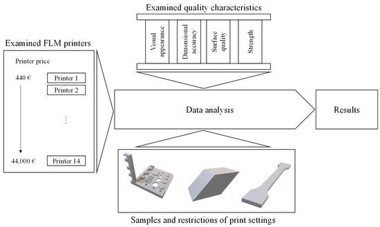
Figure 1.
Research approach.
2. Brief Literature Review
A brief literature review was performed using the words “Benchmarking”, “FLM”, “FDM”, “FFF”, “printer”, “low-cost printer”, “industrial printer”, and “desktop printer”. Publications that examined material extrusion, compared printers, considered part quality, and were published in journals or conference proceedings were considered. The evaluation was based on the title and abstract.
The current literature in the area of material extrusion has not investigated the dependence of the printer price on part quality. Related research has conducted comparisons and benchmarking of printers. Justino Netto et al. developed an approach to select an appropriate FLM printer using the analytic hierarchy process. The performed approach was used to compare three printers in the low-cost segment. The quality characteristics of the surface roughness, dimensional accuracy, and geometric accuracy were measured using a self-developed sample [14]. An adaptive benchmarking approach was developed by Spitaels et al., which was used to compare two printers [15]. Cruz Sanchez et al. performed a geometrical benchmarking of an open-source 3D printer, FoldaRap, in 2014 [16]. Karcmarcik et al. performed a comparison of the achievable accuracy of two low-cost FLM printers [17]. Galantucci et al. and Minetola et al. compared a low-cost printer and an industrial printer and found that they achieved better results with an industrial FLM printer [18,19]. The research was published in 2015, so it may be outdated, especially since the print quality in the low-cost FLM segment has improved since then.
The presented research either focuses on solely one quality characteristic, uses a highly simplified sample to examine the quality characteristics, and/or compares only a small number of printers. Accordingly, the research in this paper improved upon the existing literature in terms of (1) the number of observed printers, (2) a wider price range of compared printers, and (3) the investigation of a higher number of quality characteristics. More importantly, however, this paper (4) presents a novel investigation of the relationship between the printer price and part quality, which has not been found in the previous literature.
3. Examined Quality Characteristics and Measuring Approach
The VDI guideline 3405 defines performance criteria and associated relevant quality characteristics for additively manufactured parts [20]. This research focused on the performance criteria artistic requirements, geometric requirements, and strength requirements. The artistic requirements considered were the visual appearance and the surface roughness as representatives of the surface quality. The geometric requirement considered was the dimensional accuracy, and the strength requirements considered were the tensile strength and elongation at break. After the arrival of the samples, they were conditioned in opaque and airtight boxes for at least 24 h (see Figure 2). Firstly, the samples were inspected visually to evaluate their visual appearance. Subsequently, the samples were tested for their quality characteristics. The mean value of the quality characteristics was used for the evaluation as a measure of the average quality achieved by the printer. The standard deviation was used to evaluate the variability of the achieved quality characteristics of the printer.
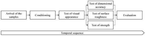
Figure 2.
Measurement procedure.
In the following, the tested quality characteristics and the restrictions to ensure the comparability of the printers are presented.
3.1. Visual Inspection
The visual appearance of the parts was verified using a direct visual inspection based on the standard DIN-EN 13018 [21]. Therefore, the samples were examined for the typical error patterns of FLM. An overview is given by the company simplify3d [22]. The occurrence of error patterns was documented after the print and conditioning phase. The recorded error patterns are visualized in Figure 3. The visual inspection was evaluated using the metric defects per unit () for all manufactured parts using the total number of defect parts and the sample size (see Equation (1)). A part was considered as defective if an error pattern was detected.
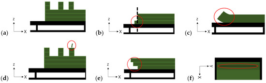
Figure 3.
Recorded error patterns via visual inspection: (a) example without error, (b) elephant foot, (c) warping, (d) stringing, (e) shifted layers and (f) gaps in thin walls.
3.2. Dimensional Accuracy
Previous publications measured the dimensional accuracy of FLM with different samples using differing characteristics and sizes [16,23,24,25,26,27,28,29]. In this paper, the dimensional accuracy was evaluated by the characteristic’s linear accuracy in the X-, Y- and Z-directions, as well as the accuracy of the holes, roundings, cylinders, and wall thicknesses in the X–Y-orientation. Therefore, a sample was developed that combined all characteristics into one sample (see Figure 4). The linear orientation was based on the linear sample of DIN EN ISO/ASTM 52902 [30]. The accuracy of the extruded cylinders was measured using five different diameters starting with 2 mm and increasing by 2 mm up to 10 mm. The same approach was used to measure the diameter of the holes. The rounding of edges was tested using a cuboid with three roundings of 2 mm, 4 mm, and 6 mm. Additionally, a 10 mm rounding was located at the outer edge of the sample. The accuracy of the walls was measured using five walls of 0.4 mm, 0.8 mm, 1.2 mm, 1.6 mm, and 2.0 mm in thickness. Some printers in the study used a nozzle diameter greater than 0.4 mm. Therefore, for the later comparison of the printers, only walls from a 1.2 mm thickness were considered. This procedure was according to VDI 3405, page 3.4, which recommends a minimum wall thickness of greater than 1 mm and twice the filament width [20].
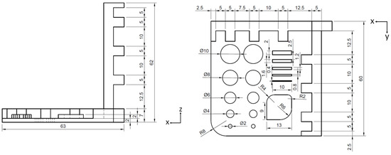
Figure 4.
Dimensional accuracy sample.
The described characteristics were measured with an optical microscope VHX-5000 from Keyence with an accuracy of 0.001 mm. The deviations from the actual dimension to the targeted dimension were measured by the length of the intervals, diameters, and radii using the software of the microscope.
The accuracy in the X- and Y-directions was measured using a chain measurement of the nine intervals. The accuracy in the Z-direction was measured with seven intervals, since the used microscope did not allow measuring the Z-bar as the required distance for optical focus was too small. The Z-bar was, therefore, gently cut with a side cutter in Interval 2 and without putting pressure on the part to prevent deformation. The evaluation of the accuracy was performed based on the percentage of absolute deviations of the targeted dimension and the actual dimension. The measuring features are marked in Figure 5.
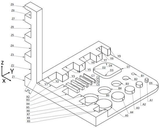
Figure 5.
Dimensional accuracy sample with marked measuring features: linear accuracy in (X, Y, and Z), cylinders (A), holes (B), wall thicknesses (C), and radii (D).
3.3. Surface Roughness
The surface roughness was measured using based on the standard DIN EN ISO 21920 [31]. The surface roughness measurement was performed orthogonal to the deposited strand (see Figure 6). The developed sample—with a parallelepiped shape—allowed measuring the surface quality of the bottom surface (Surface 3), top surface (Surface 4), two straight surfaces in the X-direction (Surfaces 2 and 5), a 45° overhang (Surface 6), and a 45° build-up (Surface 1). The sample and the naming of the surfaces are shown in Figure 7.
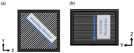
Figure 6.
Measuring direction orthogonal to the deposited strands for (a) top and bottom surface and (b) surfaces within the build direction.
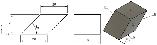
Figure 7.
Surface roughness sample and naming of the surfaces.
The surface was measured using the tactile measuring device Hommel-Etamic T8000Rc with a machine accuracy of ±0.001 mm for and ±0.003 mm for . A diamond tip with a probe tip radius of 0.005 mm was used. The achieved surface quality was compared based on the average and the scatter of these based on the standard deviation.
3.4. Strength
This paper investigated the tensile strength and elongation at break. Therefore, a flat sample of Type A1 according to DIN EN ISO 527-1 [32] and 3167 [33] was used with a length of 150 mm (see Figure 8). A horizontal orientation (XYZ-orientation) with a centered positioning was used. The samples were tested using an Inspekt 200 from Hegewald & Peschke Meß- und Prüftechnik GmbH with a load cell of 10 kN, a test speed of 3 mm/min, a break-off criterion of 75%, and a safety criterion of 8 kN. The machine has an accuracy of traversing measurement of 0.0012 μm. The samples were marked with a graphite pencil before testing (see Figure 9). The achieved tensile strength and elongation at break, as well as their scatter—measured with the standard deviation—were analyzed. The observations were performed based on Acrylonitrile Butadiene Styrene (ABS) materials. Different material manufactures could not be avoided as a result of manufacturer-related material restrictions and the different filament diameters needed. The resulting limitation and effects on the strength characteristics are discussed in Section 6.5.
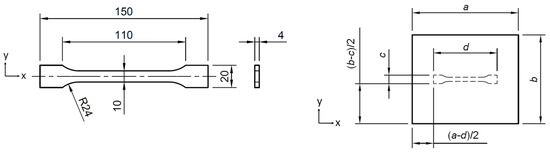
Figure 8.
Dimensions of tensile sample and top view of the positioning.
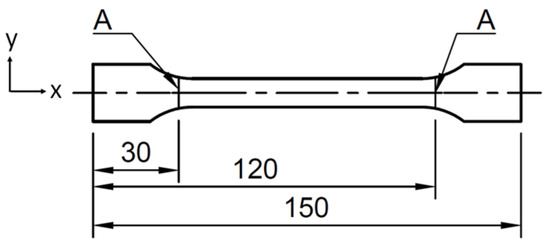
Figure 9.
Markers for the measurement of the elongation at break.
4. Methodology of Regression Analysis
A regression analysis was used to observe the correlation of the printer price and quality characteristics. For the regression approach, linear (Equation (2)), exponential (Equation (3)), and power functions (Equation (4)) were used with the constants and . The purpose of this study was to investigate if the quality of a printer can be a function of the printer price, i.e., there is a dependence. Therefore, the print quality () is the variable to be explained and the independent variable is the printer price (). In other words, the goal was to explain the print quality using the printer price.
The regression analysis was performed using RStudio. The results of the regressions are reported in a table that includes the variables, sample sizes, , adjusted , the residual standard error, and the F-statistic. This table follows the American Sociological Review standard. The goodness-of-fit was evaluated using the coefficient of determination () [34]. First, the data were analyzed visually and the achieved s were compared. For regressions with a noticeable trend, a detailed analysis was performed. The significance of the results was evaluated using the F-statistic with the corresponding p-value. The distribution of the residuals was analyzed using a Quantile–Quantile Plot (Q–Q-plot) [35]. The scatter of the residuals was evaluated by comparison of the fitted values and the residuals. Finally, outliers are detected using Cook’s distance. These characteristics were used to determine whether the quality characteristic correlated with the price of the printer. The most important regression results are discussed within this paper. The remaining results are presented in the appendices (see Appendix A).
5. Objects of Investigation and Parameter Restrictions
5.1. Investigated Printers
Table 1 provides an overview of the printers observed. The purchase price of the printers ranged from 440 to 44,000 euros. The current unnegotiated printer price of the used printer in euro provided by the printer manufacturer or a specialist retailer was used. The printers observed had build volumes ranging from 5,832,000 mm3 to 90,000,000 mm3, with more expensive printers tending to have larger build volumes. The observed printers with the respective machine manufacturer and the manufacturer of the samples are stated in Table 2. The samples were either manufactured by a printer manufacturer or specialist retailer on a machine that was used to produce test prints, or printed by a user operating the machine in its current state.

Table 1.
Comparison of the investigated printers.
Table 2.
Overview of printers sorted by price.
The observed printers differed in machine age. However, despite that care was taken that the printers were in a maintained condition, it should be mentioned that the used technical solutions of aged printers differ from current published. Printer manufacturers and special retailers printed on printers exclusively used to provide test samples. It was assumed that these printers were in the current state despite that the machine age was unknown.
5.2. Restrictions and Deviations of Print Settings
Parameter restrictions were made to ensure comparability as the process parameters affected the resulting part quality. The parameter specifications given in Table 3 were mandatory. Deviations from these were based on machine-dependent reasons. In the case of a deviation, the closest-possible parameter value the printer allowed was used. Parameters that were not classified as mandatory could be selected by the machine operator in such a way that, from their point of view, the best-possible result could be achieved. This paper used the Slicer software provided by the printer manufacturer. This ensured that the parameters used were those intended by the machine manufacturer and within the machine limits. For example, parameters such as print speed depend on the nozzle location and printer mechanics. Therefore, speed profiles were used. Restricting such parameters would result in a possible weakening of the printers that use higher speeds as a result of a faster extrusion.
Table 3.
Overview of parameter restrictions per sample.
In the following, the deviations of this study are discussed. The layer thickness of the Fortus 250 mc (0.178 mm) and Infinity F350 (0.15 mm) deviated from the targeted 0.1 mm caused by printer limitations. For each quality characteristic, five samples were tested to gain information about the repeatability of the printer. The targeted five samples for testing were met with two exceptions. For the I500, four samples, and for the EL-40, three samples were tested as no more samples were provided. However, it is not believed that these minor variations affected the findings of this study.
6. Results
6.1. Visual Appearance
By the visual inspection, 48 defective parts with at least one error were detected. Based on the five detected error patterns (see Figure 10), the visual inspection identified 74 errors. The dimensional accuracy sample resulted in the most detected errors (42). The surface roughness (28 errors) and tensile strength samples (4 errors) seemed to be less vulnerable to print errors.
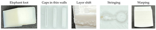
Figure 10.
Exemplary pictures of the detected error patterns.
Multiple print errors could be detected, especially for printers with a price below EUR 1000 (see Figure 11). Nevertheless, some printers below EUR 5000 had a low DPU. In the industrial printer segment (EUR > 5000), two printers resulted in a DPU higher than 0. However, one printer above EUR 10,000 had a machine age of 5 years, indicating that it might be outdated compared to the current existing printers.
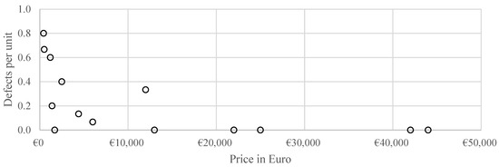
Figure 11.
Parts with a detected error in correlation with the printer price.
The regression results are shown in Table 4. In the performed investigations, the power function resulted in the highest of 0.56 with a low p-value (under 0.01). The plots for the detailed investigation of the regression are shown in Figure 12. The regression function already showed a strong negative slope at low printer prices and approached a DPU of 0 with increasing printer prices (see (a) in Figure 12). The Q–Q plot showed a nearly linear behavior, indicating that Gaussian-distributed residuals can be assumed (see (b) in Figure 12). The standardized residuals scattered around zero and had values ranging from 2 to −3, with only two outliers outside the range of 1 to −1. The data points with a high fitted value fluctuated significantly less. It can be seen that there were only a few data points above a fitted value of 0.4. This was caused by the dataset, as only three printers had a DPU higher than 0.4. Two data points had a significantly higher Cook’s distance compared to the others. This indicates that these points had a significant impact on the regression analysis. The X1-Carbon (ID 5) resulted in 0 DPU and had a printer price of EUR 1700. The printer performed better than other printers with similar prices. The EL-11 (ID 9) performed worse than the printers with similar prices (DPU of 0.33).
Table 4.
Regression results by the correlating printer price and defects per unit.
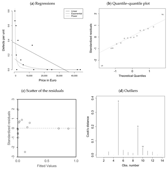
Figure 12.
Regression analysis of defects per unit by printer price with a power function.
The analysis showed that the data examined can be approximated by a power function. Therefore, it can be assumed that the DPU depends on the printer price, i.e., there is a correlation between defective parts and the printer price.
6.2. Dimensional Accuracy
The measured deviations of the lengths from the targeted value of the intervals in the X- and Y-directions had a smaller interquartile range than the intervals in the Z-direction (compare (a) and (b) to (c) in Figure 13). The difference between the equal intervals in the X- and Y-directions was on average 1.46%, indicating a low deviation between the two directions. The mean deviations of the Z-direction to X (3.79%) and Y (3.87%) were higher. The cylinders had a lower interquartile range of the percentage of deviations (2.00%) than the holes (3.68%). In the performed investigations, the mean absolute deviation between the holes and cylinders was 3.54%. The percentage deviations of the wall thicknesses had outliers with high values (see (f) in Figure 13). These were caused mainly by wall thicknesses of 0.4 mm and 0.8 mm (measuring intervals C1 and C2). As discussed, in further investigations, the wall thickness was solely evaluated by measuring distances C3, C4, and C5.
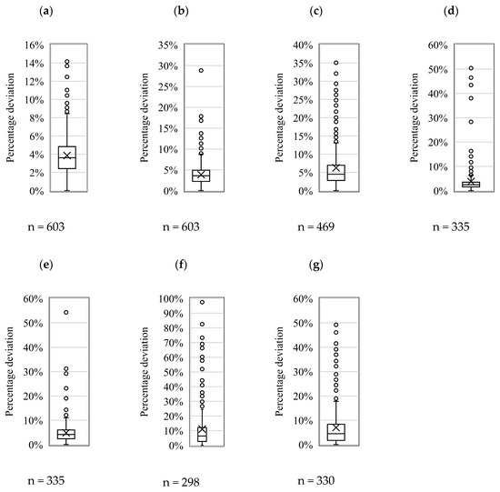
Figure 13.
Box plots of the percentage deviation of all measured samples for the (a) X-direction, (b) Y-direction, (c) Z-direction, (d) cylinders, (e) holes, (f) wall thicknesses, and (g) roundings with the number of measurements (n), outliers (circles), and mean values (crosses) marked.
The dimensional accuracy was evaluated based on the mean percentage dimensional deviation of each characteristic shown in Figure 14. For all characteristics examined, printers priced below EUR 5000 were identified that achieved similar dimensional deviations to more-expensive printers (see Figure 14). The accuracy achieved by the low-cost printers varied more for the Z-direction, cylinders, holes, wall thicknesses, and roundings (see Figure 14). For the X-direction and Y-direction, low-cost printers had mostly similar or lower percentage dimensional deviations compared to more-expensive printers (see (a) and (b) in Figure 14).
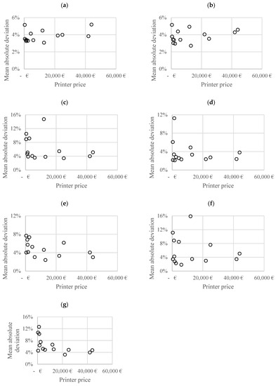
Figure 14.
Dimensional accuracy in relation to the printer price: (a) X-direction, (b) Y-direction, (c) Z-direction, (d) cylinders, (e) holes, (f) wall thicknesses, and (g) roundings.
The regression analysis of feature roundings had an R2 value of 0.46, suggesting a potential relationship worthy of further investigation. For the other features, low R2 values were achieved, indicating that the relationship between the dimensional accuracy characteristics and the printer price could not be explained well by the chosen regression method (see Table 5).
Table 5.
Best achieved goodness-of-approximation () of the dimensional accuracy measured with the mean percentage dimensional deviation.
The power function yielded a low p-value of less than 0.01, indicating the statistical significance of the results (see Table 6). The regression line had an initial slope in the low-cost range, with decreasing dimensional deviations as printer price increased (see (a) in Figure 15). However, data points were identified in the low-cost range that exhibited dimensional deviations on par with the most-expensive printers and, therefore, fell below the regression line. The Q–Q plot showed a nearly linear behavior, suggesting that the residuals could be assumed to follow a Gaussian distribution (see (b) in Figure 15). The scatter plot of the residuals showed no discernible patterns, indicating that the regression model was appropriate for the data (see (c) in Figure 15). Using Cook’s distance, ID 2 was identified as the most-influential case (see (d) in Figure 15). The low-cost printer Prusa Mini+ (ID 2) achieved significantly lower average deviations compared to other printers in the low-cost price segment, with an average dimensional deviation of 4.58%. As such, it strongly influenced the regression analysis and can be considered an outlier. In addition, ID 11 had a significant deviation below the regression curve and achieved the lowest percentage deviation, while ID 3 had a higher dimensional deviation and was an outlier. However, it is important to note that outlier ID 2 had a higher impact on the regression compared to ID 11 and ID 3.
Table 6.
Regression results by correlating the printer price and average deviation of the roundings.
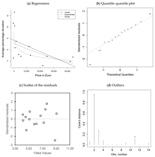
Figure 15.
Regression analysis of mean percentage deviation of the roundings with the power function.
The analysis indicated that a relationship between the average accuracy of the roundings and printer price could be identified using a power function. This suggests that the dimensional deviations of the roundings tend to decrease as the printer price increases.
In the following, the standard deviation of the dimensional deviations is investigated. In the X- and Y-directions, the standard deviations did not differ significantly with respect to the printer price, mostly below 3% (see (a) and (b) in Figure 16). In the Z-direction, larger variations were observed for printers priced below EUR 20,000 (see (c) in Figure 16). Nevertheless, low-cost printers achieved comparable or even lower standard deviations in the performed study. The standard deviations of the cylinders and holes were generally less than 4%, except for two low-cost printers (see (d) and (e) in Figure 16). The variation in the wall thickness deviated throughout the observed printer prices, suggesting that the observed variation is not influenced by the printer price (see (f) in Figure 16). However, there was a decreasing trend in the standard deviation for roundings, although some low-cost printers achieved similar or equivalent levels of variation to the more-expensive printers (see (g) in Figure 16).
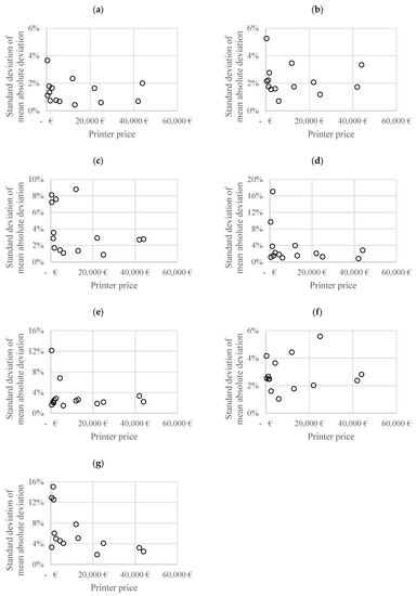
Figure 16.
Scatter of the dimensional accuracy of the features in relation to the printer price: (a) X-direction, (b) Y-direction, (c) Z-direction, (d) cylinders, (e) holes, (f) wall thicknesses, and (g) roundings.
The regression analysis of the roundings achieved an R2 value over 0.2 (see Table 7). Consequently, the regression models of the other characteristics were not further investigated, as no relationship between the printer price and quality characteristics could be assumed.
Table 7.
Best achieved goodness-of-approximation () of the scatter of the dimensional accuracy measured with the mean percentage deviation.
For the roundings, a power function achieved an R2 of 0.410, while an exponential function yielded an R2 of 0.386. Both achieved a p-value under 0.05 (see Table 8). The regression using the power function was analyzed in more detail as it achieved a higher R2. The regression line generated by the power function exhibited a low slope at lower printer prices, gradually flattening out as the prices increased ((a) in Figure 17). Low-cost printers could be identified with deviations under the regression line. The Q–Q plot deviated from the expected straight line, indicating that the residuals did not follow a Gaussian distribution ((b) in Figure 17). This suggests that either (a) the regression using the power function does not accurately reflect the relationship of standard deviation and price, (b) heteroscedasticity exists, i.e., non-constant variance of the residuals, or (c) outliers and missing data are present. However, the residuals themselves scattered around the zero line without any discernible pattern, and the standardized residuals ranged between −3 and 2 (see (c) in Figure 17). This indicates homoscedasticity, thereby excluding heteroscedasticity as a concern.
Table 8.
Regression results by correlating the printer price and standard deviation of the accuracy deviations of the roundings.
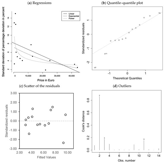
Figure 17.
Regression analysis of the standard deviation of the accuracy deviations of the roundings with the power function.
The previously identified influential cases for the regression of the average dimensional deviations—ID 2, ID 3, and ID 11—were also identified in the analysis of the standard deviations ((d) in Figure 17). ID 2 achieved a low standard deviation compared to printers of similar prices, while ID 3 exhibited a higher standard deviation. ID 11 recorded the lowest measured variation, with a standard deviation of 1.90%.
Overall, the analysis indicated that the relationship between the variation of the accuracy deviations of the roundings and printer price cannot be adequately captured through the power function. This could indicate either the absence of such a relationship or insufficient data availability. As a result, for all examined quality characteristics, no significant correlation between the variation of quality and the printer price could be identified.
6.3. Surface Roughness
The following investigations targeted the surface roughness measured in . Among the samples examined, Surfaces 1 (build-up orientation), 2 (vertical orientation), 4 (top side), and 5 (vertical orientation) achieved interquartile ranges of less than 7 μm, indicating low variation among the printers (see Figure 18). In contrast, Surfaces 3 (bottom side) and 6 (overhang) showed greater variation, with interquartile ranges of 9.17 μm and 16.58 μm, respectively. Outliers were observed for Surfaces 1, 2, and 3.
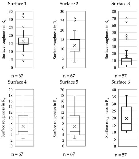
Figure 18.
Box plots of the measured surface roughness with the number of measurements (n), outliers (circles), and mean value (crosses) marked.
For the bottom surface, Printer ID 10 and ID 13 achieved significantly higher surface roughness than the other printers, exceeding 40 μm. Therefore, they could be identified as outliers (see Surface 3 in Figure 18). Printer ID 1 and ID 2 had surface roughness deviations greater than 400 μm for Surfaces 3 (bottom side) and 6 (overhang). Therefore, the peak-to-valley differences exceeded the limit of the testing machine. As a result, these printers were excluded from further analysis for these specific surfaces as no surface roughness could be measured.
In the study, some printers from the low-cost segment were able to achieve lower surface roughness across all surface orientations than more-expensive ones (see Figure 19). For Surfaces 2 and 5, which have the same orientation, the data points had minor deviations from each other (mean of 1.08 μm and standard deviation of 0.93 μm). Three printers—ID 10, ID 12, and ID 13—achieved the highest surface roughness at the bottom side (Surface 3) while five printers achieved the lowest—ID 5, ID 6, ID 7, ID 11, and ID 14. However, it should be noted that the type of build platform affected the surface roughness of Surface 3, so the differences could be caused by different types of build platforms due to the design of the printer. It is noticeable that two printers outside the low-cost segment displayed higher average surface roughness compared to the other printers.
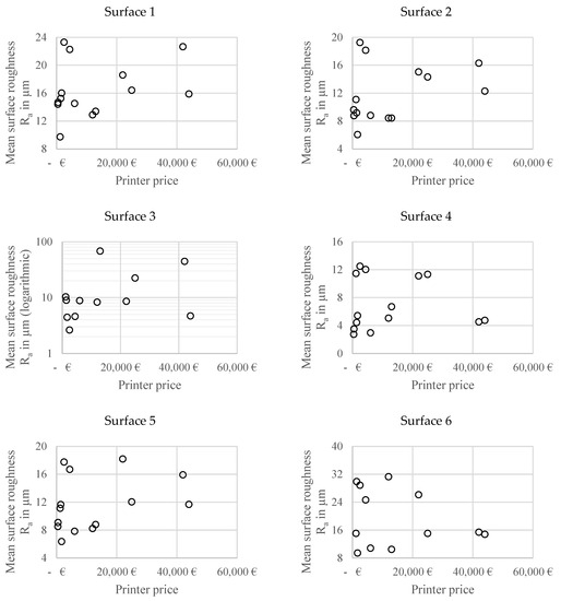
Figure 19.
Measured mean surface roughness (Surface 3 in a logarithmic visualization).
The measured mean surface roughness of each printer in Figure 19 indicates that no correlation between the average surface roughness and the printer price can be identified. This finding was supported by the regression analysis, which yielded low R2 values below 0.20 (see Table 9). As a result, a detailed regression analysis of the relationship between surface roughness and printer price was deemed not purposeful.
Table 9.
Best achieved goodness-of-approximation (R2) of the surface roughness measured with the mean Ra.
Furthermore, the standard deviation of the surface roughness and its relationship with the printer price were investigated. The measured standard deviation remained below 7 μm. Different standard deviations for similar printer prices were observed for all surfaces, regardless of whether the printer belonged to the low-cost segment or not (see Figure 20). In Figure 20, no discernible correlation between the scatter of the surface roughness and printer price could be identified. The regression analysis resulted in low R2 values, thus lacking significant explanatory power (see Table 10).
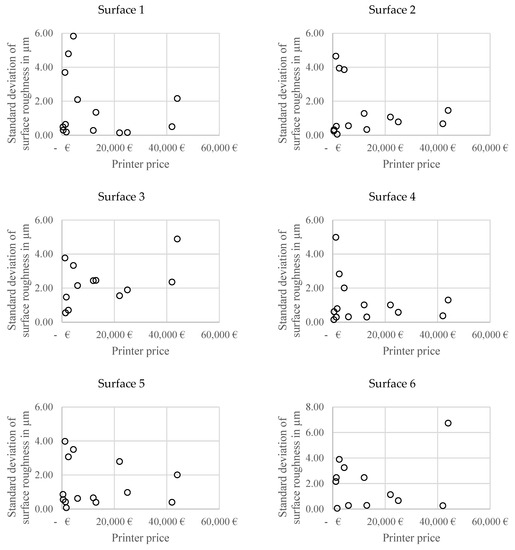
Figure 20.
Measured standard deviation of surface roughness.
Table 10.
Best achieved goodness-of-approximation (R2) of the standard deviation of surface roughness.
Overall, the findings suggested that printers from the low-cost segment were capable of achieving comparable surface roughness compared to higher-priced printers. No significant dependency between surface roughness and printer price could be identified based on the available data. It should be noted that the two printers with the lowest price could not be considered for Surfaces 3 and 6. However, it was not assumed that the consideration of these printers would have contributed to the identification of a dependency, as the values recorded were highly scattered, regardless of the printer price.
6.4. Strength
The strength samples of the observed printers had a differing breaking behavior. Most samples broke with a nearly linear (see the samples of Printer ID 2, ID 5, and ID 9 to ID 14 in Figure 21) or a nonlinear cut (see the samples of Printer ID 6 to ID 8 in Figure 21). The different breaking behavior could be recognized in the stress–strain diagram (compare (a) and (b) in Figure 22). Samples of some printers had a delamination of the infill and the surrounding perimeters while performing the strength test, although all strands were printed in the direction of pull. The delamination could be recognized especially for the low-cost printer segment (see Printer ID 1, ID 3, and ID 4 in Figure 21). This caused a change in the stress–strain curve (compare (a) and (c) in Figure 21), and the sample had higher strain values.
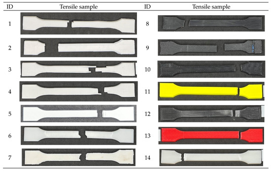
Figure 21.
Broken strength samples in descending order of the printer price marked with the printer ID.
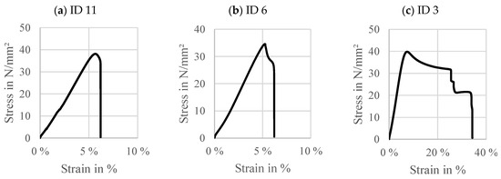
Figure 22.
Stress–strain curve of (a) a linear break, (b) a nonlinear break, and (c) a break with layer separation.
The tensile strength samples had a range of 43.19 N/mm2 with an interquartile range of 4.14 N/mm2. The maximum tensile strength achieved was 47.33 N/mm2 (see (a) in Figure 23). A noticeable variation in the mean tensile strength was observed among the printers within similar price ranges, regardless of the low-cost segment (see (a) in Figure 24). The standard deviation of the tensile strength remained below 6 N/mm2 for all printers. In particular, printers priced above EUR 20,000 showed a standard deviation below 1 N/mm2 (see (b) in Figure 24). While some lower-cost printers also achieved this level of variation, other printers below the EUR 20,000 threshold had a higher standard deviation, i.e., their samples varied to a greater extent.
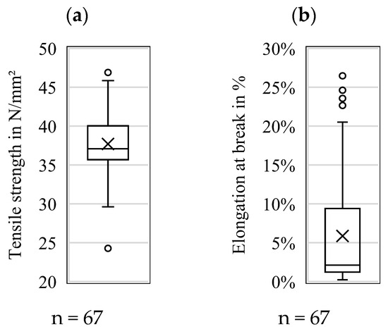
Figure 23.
Distribution of measured (a) tensile strength and (b) elongation at break of all samples.
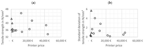
Figure 24.
Mean values of (a) tensile strength and (b) standard deviation of tensile strength in reference to the printer price with matching material (triangles) and single used materials (points) marked.
The measured elongation at break had an interquartile range of 7.4% and a range of 26.2% (see (b) in Figure 23). The highest elongations at break were measured in the low-cost segment. A decrease in elongation at break was observed with increasing printer price (see (a) in Figure 25). Overall, the standard deviation of the elongation at break was less than 7% (see (b) in Figure 25). For printers priced above EUR 10,000, the standard deviation was consistently below 1.5%, except for one printer (see (b) in Figure 25). A higher variation in the low-cost segment compared to higher-priced printers could be identified (see (b) in Figure 25).
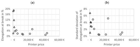
Figure 25.
Mean values of (a) elongation at break and (b) standard deviation of elongation at break with reference to the printer price with matching material (triangles) and single used materials (points) marked.
The regression analysis of the tensile strength showed low R2 values of less than 0.10%, indicating a poor fit of the regression models (see Table 11). Therefore, further investigation of this was not pursued. In contrast, the regression analysis of the elongation at break yielded an R2 value of 0.472 and, for the associated standard deviation, an R2 value of 0.321. Therefore, a more-detailed analysis was performed.
Table 11.
Best achieved goodness-of-approximation (R2) of the tensile strength and elongation at break and their standard deviations.
The elongation at break appeared to have a power function behavior (see (a) in Figure 26). The p-value was less than 0.01, indicating statistical significance (see Table 12). The residuals are nearly linearly distributed, indicating non-Gaussian-distributed residuals (see (b) in Figure 26). A relatively uniform distribution was observed, and the standardized residuals ranged between 2 and −3 (see (c) in Figure 26). Therefore, heteroscedasticity was not assumed to be present. The influential cases ID 2, 3, and 11 could be identified as outliers (see (d) in Figure 26). Among these cases, ID 2 had a significantly lower elongation at break despite its relatively low price. Outlier ID 2 had a higher influence on the regression compared to ID 3 and ID 11. With the regression analysis, a dependence of the achieved mean elongation at break and the printer price could be identified.
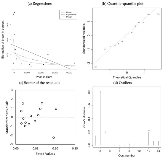
Figure 26.
Regression analysis of elongation at break.
Table 12.
Regression results by correlating the printer price and elongation at break.
The results of the regression analysis of the standard deviation of the elongation at break are shown in Table 13 with the corresponding regression functions shown in (a) in Figure 27. The power function achieved an R2 value of 0.321 and yielded a p-value below 0.05, suggesting a statistical significance of the relationship (see Table 13). The residuals were not linearly distributed, suggesting a non-Gaussian distribution (see (b) in Figure 27). Heteroscedasticity was not assumed based on the random distribution of the standardized residuals, which ranged between 2 and −2 (see (c) in Figure 27). However, with the given data, no relationship could be assumed between the standard deviation of the elongation at break and the printer price. Based on the available data, it can be assumed that either no significant relationship exists or the current dataset is insufficient to accurately capture the underlying relationship. If, contrary to the performed analysis, a relationship is suspected, additional data would need to be collected.
Table 13.
Regression results by correlating the printer price and standard deviation of elongation at break.
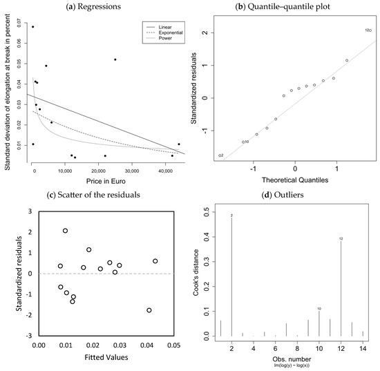
Figure 27.
Regression analysis of the standard deviation of elongation at break.
6.5. Critical Appraisal of the Results
The results of this study were limited to the ABS material. A printer comparison for materials with a differing printability, such as Polylactic Acid (PLA) or Glycol-modified Polyethylene Terephthalate (PETG), could differ from the results obtained. As mentioned, differing material manufactures could not be avoided as a result of manufacturer-related material restrictions and the different filament diameters needed. Due to different mixing ratios in the production of the ABS material and the different colors of the filaments, the behavior of the tensile strength and elongation at break may differ to a certain extent from other ABS materials. This could reduce the accuracy of the strength tests.
The investigations of this paper were based on parameter restrictions in order to be able to compare the printers with each other. Therefore, the quality reached does not represent the maximum achievable. Improvements in part quality, based on parameter tuning or ironing through a heated nozzle, were not considered.
The part quality depends on the sample complexity, which is why the findings of this paper were limited to the complexity of the described samples. Should a higher complexity be required, the printability for the particular printer would have to be proven before the results of this investigation could be used.
The performed investigations of the dependence of the part quality and the printer price were limited by the approximation functions: linear, exponential, and power function. Therefore, further tests should be performed if more-complex dependencies are suspected. However, the investigations of this research indicate that more-complex dependencies are not to be expected.
In this research, the low-cost printer segment was studied more deeply. Therefore, at high printer prices, the approximation was affected by a few printers, which could cause some inaccuracy in the approximation. The studied printers differed in price and machine age. Care was taken to ensure that the printers were in a maintained condition to reduce the influence of machine age on the print process. However, a certain extent of inaccuracy could be caused by aged printers as a result of older technical solutions in the print process. In particular, Printer ID 9 may be outdated as it lacks the DPU and dimensional accuracy of the even older Printers ID 7 and ID 11.
The investigations focused on part quality and printer price. Thus, other factors, e.g., print time, material costs, labor costs, costs for preprocessing and postprocessing, energy costs, and maintenance costs were neglected. Differences in printer manufacturer support, printer connectivity, and the effort required to connect the printer to the existing production environment were not considered. The printer price was strongly, yet not solely, influenced by the achievable part quality. Therefore, printers with higher prices based on other attributes, such as print speed or material variety, could introduce inaccuracies into the correlation approach.
The purpose of the study was to identify a relationship between the printer price and part quality characteristics. Therefore, the regressions developed were not intended for predictive use. Use for prediction would require more data to improve the R2 value.
The stated results, observed correlations, and findings are not expected to be compromised by the limitations and imprecision of the research design.
7. Conclusions
In this paper, the part quality—in detail, the visual appearance, dimensional accuracy, surface roughness, and strength—of 14 FLM printers with differing prices were examined using the ABS material and three test samples. The relationship between the printer price and part quality was investigated.
In the following, the main research questions of this paper—mentioned in the Introduction—are answered:
(1) A relationship between the printer price and part quality could be identified. However, the price of the printer cannot be used as an indicator of the part quality beyond the number of defects, the elongation at break, and the accuracy of the roundings. A relationship between the printer price and the surface roughness, tensile strength, and other dimensional accuracy characteristics could not be identified. Thus, in the performed observations, a more-expensive printer was not generally associated with an increase in all observed part quality characteristics. No improvement in the standard deviation, e.g., less variation in part quality, could be observed with a higher printer price.
(2) All of the regression lines that identified a relationship between part quality and printer price had sharp drops at low printer prices, indicating that even low-cost printers achieve satisfactory quality in these characteristics. Since the other characteristics were independent of the part quality and since some low-cost printers were found to have a similar quality as more-expensive printers, the study showed that low-cost printers under EUR 5000 can compete with more-expensive printers.
(3) Printers below EUR 1000 had a significantly higher DPU and high peak-to-valley differences in the surface roughness testing, resulting in non-measurable surfaces. The results indicated that the low-cost printer segment should be divided into printer prices below EUR 1000—indicating a part quality not suitable for industrial applications—and between EUR 1000 and 5000—indicating a part quality that could be suitable for industrial applications.
When selecting a suitable printer, it is recommended to determine a minimum printer price by using the characteristics of the defects per unit, elongation at break, and the accuracy of the roundings. Subsequently, other quality characteristics can be compared within the price range as they are independent of the printer price. The results indicated that the quality characteristics of the more-expensive printers (EUR > 40,000) were closer to each other than those of the other observed printers. This could lead to less testing in the selection process.
Future work is planned to investigate the influence of different materials such as PETG and part complexity on the study performed. Further integration of printers above EUR 20,000 and newly released printers is planned. Furthermore, predicting the quality characteristics in relation to the process parameters, printers, and materials is targeted. An accurate prediction could allow the use of low-cost printers in the business environment since the price of the printer does not necessarily correlate with a higher part quality.
Author Contributions
Conceptualization, C.S., R.G., J.T.S. and F.F.; methodology, C.S., R.G., J.T.S. and F.F.; data collection, C.S. and A.M.; analysis, C.S.; writing—original draft preparation, C.S.; writing—review and editing, R.G., F.F., J.T.S. and C.S.; visualization, C.S.; supervision, F.F. and J.T.S. All authors have read and agreed to the published version of the manuscript.
Funding
This research received no external funding.
Data Availability Statement
Data from this paper are available upon request from the authors.
Acknowledgments
The authors express their thanks to the Institute for Functional Interfaces (IFG) at the Karlsruhe Institute of Technology and the Laboratory for Materials Testing at the Karlsruhe University of Applied Sciences for granting us access to their measuring equipment.
Conflicts of Interest
The authors declare no conflict of interest.
Appendix A
Table A1.
Regression results of the average deviation in the X-direction.
Table A1.
Regression results of the average deviation in the X-direction.
| y | |||
|---|---|---|---|
| Linear | Exponential | Power | |
| a | 0.000 | 1.000 | 0.023 |
| b | 3.621 *** | 3.586 *** | 3.124 *** |
| N | 14 | 14 | 14 |
| R2 | 0.166 | 0.175 | 0.047 |
| Adjusted R2 | 0.097 | 0.106 | −0.033 |
| Residual Std. Error (df = 12) | 0.648 | 0.158 | 0.17 |
| F-Statistic (df = 1; 12) | 2.39 | 2.544 | 0.588 |
* p < 0.05; ** p < 0.01; *** p < 0.001.
Table A2.
Regression results of the average deviation in the Y-direction.
Table A2.
Regression results of the average deviation in the Y-direction.
| y | |||
|---|---|---|---|
| Linear | Exponential | Power | |
| a | 0.000 | 1.000 | 0.016 |
| b | 3.643 *** | 3.572 *** | 3.290 ** |
| N | 14 | 14 | 14 |
| R2 | 0.089 | 0.099 | 0.016 |
| Adjusted R2 | 0.013 | 0.024 | −0.066 |
| Residual Std. Error (df = 12) | 0.748 | 0.194 | 0.203 |
| F-Statistic (df = 1; 12) | 1.171 | 1.323 | 0.192 |
* p < 0.05; ** p < 0.01; *** p < 0.001.
Table A3.
Regression results of the average deviation in the Z-direction.
Table A3.
Regression results of the average deviation in the Z-direction.
| y | |||
|---|---|---|---|
| Linear | Exponential | Power | |
| a | 0.000 | 1.000 | −0.107 |
| b | 6.879 *** | 6.129 *** | 13.681 ** |
| N | 14 | 14 | 14 |
| R2 | 0.066 | 0.077 | 0.131 |
| Adjusted R2 | −0.012 | 0.000 | 0.058 |
| Residual Std. Error (df = 12) | 3.398 | 0.464 | 0.451 |
| F-Statistic (df = 1; 12) | 0.848 | 0.995 | 1.807 |
* p < 0.05; ** p < 0.01; *** p < 0.001.
Table A4.
Regression results of the average deviation of the cylinders.
Table A4.
Regression results of the average deviation of the cylinders.
| y | |||
|---|---|---|---|
| Linear | Exponential | Power | |
| a | 0.000 | 1.000 | −0.075 |
| b | 4.179 *** | 3.511 *** | 6.184 * |
| N | 14 | 14 | 14 |
| R2 | 0.050 | 0.031 | 0.061 |
| Adjusted R2 | −0.029 | −0.050 | −0.017 |
| Residual Std. Error (df = 12) | 2.483 | 0.486 | 0.478 |
| F-Statistic (df = 1; 12) | 0.635 | 0.385 | 0.784 |
* p < 0.05; ** p < 0.01; *** p < 0.001.
Table A5.
Regression results of the average deviation of the holes.
Table A5.
Regression results of the average deviation of the holes.
| y | |||
|---|---|---|---|
| Linear | Exponential | Power | |
| a | 0.000 | 1.000 | −0.122 |
| b | 5.442 *** | 5.165 *** | 12.845 *** |
| N | 14 | 14 | 14 |
| R2 | 0.191 | 0.181 | 0.278 |
| Adjusted R2 | 0.123 | 0.112 | 0.218 |
| Residual Std. Error (df = 12) | 1.598 | 0.343 | 0.322 |
| F-Statistic (df = 1; 12) | 2.824 | 2.646 | 4.616 |
* p < 0.05; ** p < 0.01; *** p < 0.001.
Table A6.
Regression results of the average deviation of the wall thicknesses.
Table A6.
Regression results of the average deviation of the wall thicknesses.
| y | |||
|---|---|---|---|
| Linear | Exponential | Power | |
| a | 0.000 | 1.000 | −0.029 |
| b | 6.168 ** | 4.835 *** | 6.098 |
| N | 14 | 14 | 14 |
| R2 | 0.011 | 0.001 | 0.005 |
| Adjusted R2 | −0.071 | −0.082 | −0.078 |
| Residual Std. Error (df = 12) | 4.206 | 0.671 | 0.670 |
| F-Statistic (df = 1; 12) | 0.133 | 0.013 | 0.061 |
* p < 0.05; ** p < 0.01; *** p < 0.001.
Table A7.
Regression results of the standard deviation of the average deviation in the X-direction.
Table A7.
Regression results of the standard deviation of the average deviation in the X-direction.
| y | |||
|---|---|---|---|
| Linear | Exponential | Power | |
| a | 0.000 | 1.000 | 0.023 |
| b | 3.621 *** | 3.586 | 3.124 |
| N | 14 | 14 | 14 |
| R2 | 0.166 | 0.175 | 0.047 |
| Adjusted R2 | 0.097 | 0.106 | −0.033 |
| Residual Std. Error (df = 12) | 0.648 | 0.158 | 0.170 |
| F-Statistic (df = 1; 12) | 2.390 | 2.544 | 0.588 |
* p < 0.05; ** p < 0.01; *** p < 0.001.
Table A8.
Regression results of the standard deviation of the average deviation in the Y-direction.
Table A8.
Regression results of the standard deviation of the average deviation in the Y-direction.
| y | |||
|---|---|---|---|
| Linear | Exponential | Power | |
| a | 0.000 | 1.000 | −0.077 |
| b | 2.290 *** | 2.008 ** | 3.873 |
| N | 14 | 14 | 14 |
| R2 | 0.002 | 0.000 | 0.060 |
| Adjusted R2 | −0.081 | −0.083 | −0.018 |
| Residual Std. Error (df = 12) | 1.195 | 0.513 | 0.497 |
| F-Statistic (df = 1; 12) | 0.021 | 0.001 | 0.766 |
* p < 0.05; ** p < 0.01; *** p < 0.001.
Table A9.
Regression results of the standard deviation of the average deviation in the Z-direction.
Table A9.
Regression results of the standard deviation of the average deviation in the Z-direction.
| y | |||
|---|---|---|---|
| Linear | Exponential | Power | |
| a | 0.000 | 1.000 | −0.216 |
| b | 4.509 *** | 3.36 *** | 18.174 * |
| N | 14 | 14 | 14 |
| R2 | 0.095 | 0.058 | 0.191 |
| Adjusted R2 | 0.019 | −0.020 | 0.124 |
| Residual Std. Error (df = 12) | 2.828 | 0.787 | 0.729 |
| F-Statistic (df = 1; 12) | 1.254 | 0.741 | 2.836 |
* p < 0.05; ** p < 0.01; *** p < 0.001.
Table A10.
Regression results of the standard deviation of the average deviation of the cylinders.
Table A10.
Regression results of the standard deviation of the average deviation of the cylinders.
| y | |||
|---|---|---|---|
| Linear | Exponential | Power | |
| a | 0.000 | 1.000 | −0.238 |
| b | 4.803 ** | 3.019 ** | 17.975 * |
| N | 14 | 14 | 14 |
| R2 | 0.101 | 0.118 | 0.190 |
| Adjusted R2 | 0.026 | 0.045 | 0.123 |
| Residual Std. Error (df = 12) | 4.413 | 0.840 | 0.805 |
| F-Statistic (df = 1; 12) | 1.347 | 1.610 | 2.817 |
* p < 0.05; ** p < 0.01; *** p < 0.001.
Table A11.
Regression results of the standard deviation of the average deviation of the holes.
Table A11.
Regression results of the standard deviation of the average deviation of the holes.
| y | |||
|---|---|---|---|
| Linear | Exponential | Power | |
| a | 0.000 | 1.000 | −0.095 |
| b | 3.825 ** | 2.897 *** | 6.073 |
| N | 14 | 14 | 14 |
| R2 | 0.049 | 0.021 | 0.069 |
| Adjusted R2 | −0.030 | −0.061 | −0.009 |
| Residual Std. Error (df = 12) | 2.904 | 0.585 | 0.570 |
| F-Statistic (df = 1; 12) | 0.618 | 0.254 | 0.890 |
* p < 0.05; ** p < 0.01; *** p < 0.001.
Table A12.
Regression results of the standard deviation of the average deviation of the wall thicknesses.
Table A12.
Regression results of the standard deviation of the average deviation of the wall thicknesses.
| y | |||
|---|---|---|---|
| Linear | Exponential | Power | |
| a | 0.000 | 1.000 | 0.002 |
| b | 2.719 *** | 2.484 *** | 2.557 |
| N | 14 | 14 | 14 |
| R2 | 0.011 | 0.013 | 0.000 |
| Adjusted R2 | −0.071 | −0.069 | −0.083 |
| Residual Std. Error (df = 12) | 1.272 | 0.454 | 0.457 |
| F-Statistic (df = 1; 12) | 0.138 | 0.162 | 0.000 |
* p < 0.05; ** p < 0.01; *** p < 0.001.
Table A13.
Regression results of the surface roughness for Surface 1.
Table A13.
Regression results of the surface roughness for Surface 1.
| y | |||
|---|---|---|---|
| Linear | Exponential | Power | |
| a | 0.000 | 1.000 | 0.048 |
| b | 15.487 *** | 15.044 *** | 10.665 *** |
| N | 14 | 14 | 14 |
| R2 | 0.082 | 0.093 | 0.097 |
| Adjusted R2 | 0.005 | 0.018 | 0.022 |
| Residual Std. Error (df = 12) | 3.951 | 0.238 | 0.238 |
| F-Statistic (df = 1; 12) | 1.065 | 1.237 | 1.289 |
* p < 0.05; ** p < 0.01; *** p < 0.001.
Table A14.
Regression results of the surface roughness for Surface 2.
Table A14.
Regression results of the surface roughness for Surface 2.
| y | |||
|---|---|---|---|
| Linear | Exponential | Power | |
| a | 0.000 | 1.000 | 0.084 |
| b | 10.712 *** | 10.044 *** | 5.490 ** |
| N | 14 | 14 | 14 |
| R2 | 0.108 | 0.145 | 0.146 |
| Adjusted R2 | 0.034 | 0.074 | 0.075 |
| Residual Std. Error (df = 12) | 4.037 | 0.332 | 0.332 |
| F-Statistic (df = 1; 12) | 1.458 | 2.041 | 2.047 |
* p < 0.05; ** p < 0.01; *** p < 0.001.
Table A15.
Regression results of the surface roughness for Surface 3.
Table A15.
Regression results of the surface roughness for Surface 3.
| y | |||
|---|---|---|---|
| Linear | Exponential | Power | |
| a | 0.000 | 1.000 | 0.327 |
| b | 10.485 | 7.156 *** | 0.5410 |
| N | 12 | 12 | 12 |
| R2 | 0.097 | 0.134 | 0.199 |
| Adjusted R2 | 0.007 | 0.047 | 0.119 |
| Residual Std. Error (df = 12) | 19.888 | 0.944 | 0.907 |
| F-Statistic (df = 1; 12) | 1.076 | 1.543 | 2.483 |
* p < 0.05; ** p < 0.01; *** p < 0.001.
Table A16.
Regression results of the surface roughness for Surface 4.
Table A16.
Regression results of the surface roughness for Surface 4.
| y | |||
|---|---|---|---|
| Linear | Exponential | Power | |
| a | 0.000 | 1.000 | 0.086 |
| b | 7.158 *** | 6.049 *** | 2.9410 |
| N | 14 | 14 | 14 |
| R2 | 0.002 | 0.001 | 0.061 |
| Adjusted R2 | −0.081 | −0.083 | −0.017 |
| Residual Std. Error (df = 12) | 3.891 | 0.571 | 0.554 |
| F-Statistic (df = 1; 12) | 0.021 | 0.009 | 0.778 |
* p < 0.05; ** p < 0.01; *** p < 0.001.
Table A17.
Regression results of the surface roughness for Surface 5.
Table A17.
Regression results of the surface roughness for Surface 5.
| y | |||
|---|---|---|---|
| Linear | Exponential | Power | |
| a | 0.000 | 1.000 | 0.076 |
| b | 10.650 *** | 10.064 *** | 5.800 ** |
| N | 14 | 14 | 14 |
| R2 | 0.102 | 0.125 | 0.128 |
| Adjusted R2 | 0.028 | 0.052 | 0.055 |
| Residual Std. Error (df = 12) | 3.897 | 0.326 | 0.326 |
| F-Statistic (df = 1; 12) | 1.370 | 1.715 | 1.759 |
* p < 0.05; ** p < 0.01; *** p < 0.001.
Table A18.
Regression results of the surface roughness for Surface 6.
Table A18.
Regression results of the surface roughness for Surface 6.
| y | |||
|---|---|---|---|
| Linear | Exponential | Power | |
| a | 0.000 | 1.000 | −0.031 |
| b | 20.992 *** | 18.746 *** | 23.453 ** |
| N | 12 | 12 | 12 |
| R2 | 0.047 | 0.019 | 0.009 |
| Adjusted R2 | −0.048 | −0.080 | −0.090 |
| Residual Std. Error (df = 12) | 8.414 | 0.457 | 0.459 |
| F-Statistic (df = 1; 12) | 0.491 | 0.189 | 0.090 |
* p < 0.05; ** p < 0.01; *** p < 0.001.
Table A19.
Regression results of the standard deviation of the surface roughness for Surface 1.
Table A19.
Regression results of the standard deviation of the surface roughness for Surface 1.
| y | |||
|---|---|---|---|
| Linear | Exponential | Power | |
| a | 0.000 | 1.000 | −0.079 |
| b | 1.969 * | 0.927 | 1.540 |
| N | 14 | 14 | 14 |
| R2 | 0.052 | 0.024 | 0.009 |
| Adjusted R2 | −0.027 | −0.058 | −0.073 |
| Residual Std. Error (df = 12) | 1.908 | 1.338 | 1.348 |
| F-Statistic (df = 1; 12) | 0.652 | 0.293 | 0.111 |
* p < 0.05; ** p < 0.01; *** p < 0.001.
Table A20.
Regression results of the standard deviation of the surface roughness for Surface 2.
Table A20.
Regression results of the standard deviation of the surface roughness for Surface 2.
| y | |||
|---|---|---|---|
| Linear | Exponential | Power | |
| a | 0.000 | 1.000 | 0.166 |
| b | 1.650 * | 0.695 | 0.1890 |
| N | 14 | 14 | 14 |
| R2 | 0.035 | 0.014 | 0.046 |
| Adjusted R2 | −0.046 | −0.069 | −0.033 |
| Residual Std. Error (df = 12) | 1.579 | 1.256 | 1.235 |
| F-Statistic (df = 1; 12) | 0.430 | 0.166 | 0.584 |
* p < 0.05; ** p < 0.01; *** p < 0.001.
Table A21.
Regression results of the standard deviation of the surface roughness for Surface 3.
Table A21.
Regression results of the standard deviation of the surface roughness for Surface 3.
| y | |||
|---|---|---|---|
| Linear | Exponential | Power | |
| a | 0.000 | 1.000 | 0.213 |
| b | 1.784 ** | 1.500 | 0.2920 |
| N | 12 | 12 | 12 |
| R2 | 0.187 | 0.186 | 0.191 |
| Adjusted R2 | 0.106 | 0.104 | 0.110 |
| Residual Std. Error (df = 12) | 1.177 | 0.607 | 0.605 |
| F-Statistic (df = 1; 12) | 2.299 | 2.281 | 2.365 |
* p < 0.05; ** p < 0.01; *** p < 0.001.
Table A22.
Regression results of the standard deviation of the surface roughness for Surface 4.
Table A22.
Regression results of the standard deviation of the surface roughness for Surface 4.
| y | |||
|---|---|---|---|
| Linear | Exponential | Power | |
| a | 0.000 | 1.000 | 0.023 |
| b | 1.421 * | 0.772 | 0.6120 |
| N | 14 | 14 | 14 |
| R2 | 0.048 | 0.003 | 0.001 |
| Adjusted R2 | −0.031 | −0.081 | −0.082 |
| Residual Std. Error (df = 12) | 1.346 | 1.021 | 1.022 |
| F-Statistic (df = 1; 12) | 0.605 | 0.031 | 0.016 |
* p < 0.05; ** p < 0.01; *** p < 0.001.
Table A23.
Regression results of the standard deviation of the surface roughness for Surface 5.
Table A23.
Regression results of the standard deviation of the surface roughness for Surface 5.
| y | |||
|---|---|---|---|
| Linear | Exponential | Power | |
| a | 0.000 | 1.000 | 0.075 |
| b | 1.528 ** | 0.836 | 0.4730 |
| N | 14 | 14 | 14 |
| R2 | 0.005 | 0.006 | 0.011 |
| Adjusted R2 | −0.078 | −0.077 | −0.071 |
| Residual Std. Error (df = 12) | 1.387 | 1.156 | 1.153 |
| F-Statistic (df = 1; 12) | 0.060 | 0.070 | 0.136 |
* p < 0.05; ** p < 0.01; *** p < 0.001.
Table A24.
Regression results of the standard deviation of the surface roughness for Surface 6.
Table A24.
Regression results of the standard deviation of the surface roughness for Surface 6.
| y | |||
|---|---|---|---|
| Linear | Exponential | Power | |
| a | 0.000 | 1.000 | −0.003 |
| b | 1.586 | 0.922 | 1.0170 |
| N | 12 | 12 | 12 |
| R2 | 0.041 | 0.003 | 0.000 |
| Adjusted R2 | −0.054 | −0.097 | −0.100 |
| Residual Std. Error (df = 12) | 2.037 | 1.507 | 1.510 |
| F-Statistic (df = 1; 12) | 0.432 | 0.029 | 0.000 |
* p < 0.05; ** p < 0.01; *** p < 0.001.
Table A25.
Regression results of the tensile strength.
Table A25.
Regression results of the tensile strength.
| y | |||
|---|---|---|---|
| Linear | Exponential | Power | |
| a | 0.000 | 1.000 | −0.004 |
| b | 37.973 *** | 37.863 *** | 38.861 *** |
| N | 14 | 14 | 14 |
| R2 | 0.005 | 0.006 | 0.005 |
| Adjusted R2 | −0.078 | −0.077 | −0.078 |
| Residual Std. Error (df = 12) | 3.555 | 0.091 | 0.091 |
| F-Statistic (df = 1; 12) | 0.057 | 0.070 | 0.055 |
* p < 0.05; ** p < 0.01; *** p < 0.001.
Table A26.
Regression results of the standard deviation of the tensile strength.
Table A26.
Regression results of the standard deviation of the tensile strength.
| y | |||
|---|---|---|---|
| Linear | Exponential | Power | |
| a | 0.000 | 1.000 | −0.018 |
| b | 1.812 ** | 1.024 | 0.9860 |
| N | 14 | 14 | 14 |
| R2 | 0.070 | 0.047 | 0.001 |
| Adjusted R2 | −0.007 | −0.033 | −0.083 |
| Residual Std. Error (df = 12) | 1.655 | 1.101 | 1.128 |
| F-Statistic (df = 1; 12) | 0.909 | 0.590 | 0.009 |
* p < 0.05; ** p < 0.01; *** p < 0.001.
References
- Wohlers, T.; Campbell, R.I.; Diegel, O.; Kowen, J.; Mostow, N.; Fidan, I. Wohlers Report 2022: 3D Printing and Additive Manufacturing: Global State of the Industry; Wohlers Associates: Fort Collins, CO, USA; Washington, DC, USA; ASTM International: West Conshohocken, PA, USA, 2022. [Google Scholar]
- DIN EN ISO/ASTM 52900; Additive Manufacturing—General Principles—Fundamentals and Vocabulary. DIN German Institute for Standardization: Berlin, Germany, 2022.
- Kechagias, J.; Chaidas, D.; Vidakis, N.; Salonitis, K.; Vaxevanidis, N.M. Key parameters controlling surface quality and dimensional accuracy: A critical review of FFF process. Mater. Manuf. Process 2022, 37, 963–984. [Google Scholar] [CrossRef]
- Dey, A.; Yodo, N. A Systematic Survey of FDM Process Parameter Optimization and Their Influence on Part Characteristics. JMMP 2019, 3, 64. [Google Scholar] [CrossRef]
- Gordelier, T.J.; Thies, P.R.; Turner, L.; Johanning, L. Optimising the FDM additive manufacturing process to achieve maximum tensile strength: A state-of-the-art review. RPJ 2019, 25, 953–971. [Google Scholar] [CrossRef]
- Mohamed, O.A.; Masood, S.H.; Bhowmik, J.L. Optimization of fused deposition modeling process parameters: A review of current research and future prospects. Adv. Manuf. 2015, 3, 42–53. [Google Scholar] [CrossRef]
- Grozav, S.D.; Sterca, A.D.; Kočiško, M.; Pollák, M.; Ceclan, V. Feasibility of Predictive Models for the Quality of Additive Manufactured Components Based on Artificial Neural Networks. Machines 2022, 10, 128. [Google Scholar] [CrossRef]
- Deshwal, S.; Kumar, A.; Chhabra, D. Exercising hybrid statistical tools GA-RSM, GA-ANN and GA-ANFIS to optimize FDM process parameters for tensile strength improvement. CIRP J. Manuf. Sci. Technol. 2020, 31, 189–199. [Google Scholar] [CrossRef]
- Bayraktar, Ö.; Uzun, G.; Çakiroğlu, R.; Guldas, A. Experimental study on the 3D-printed plastic parts and predicting the mechanical properties using artificial neural networks. Polym. Adv. Technol. 2017, 28, 1044–1051. [Google Scholar] [CrossRef]
- Vahabli, E.; Rahmati, S. Application of an RBF neural network for FDM parts’ surface roughness vol. 28, 8, 1044–1051, prediction for enhancing surface quality. Int. J. Precis. Eng. Manuf. 2016, 17, 1589–1603. [Google Scholar] [CrossRef]
- Schmidt, C.; Finsterwalder, F.; Griesbaum, R.; Sehrt, J.T. Cost Analysis of Automated Additive Printer Farms. IOP Conf. Ser. Earth Environ. Sci. 2022, 1048, 12008. [Google Scholar] [CrossRef]
- Schmidt, C.; Finsterwalder, F.; Griesbaum, R.; Sehrt, J.T. Determination of factory locations for distributed additive manufacturing, considering pollution, resilience and costs. CIRP J. Manuf. Sci. Technol. 2023, 43, 115–128. [Google Scholar] [CrossRef]
- Wohlers Associates. Wohlers Report 2017: 3D Printing and Additive Manufacturing State of the Industry: Annual Worldwide Progress Report; Wohlers Associates: Fort Collins, CO, USA, 2017. [Google Scholar]
- Netto, J.M.J.; Ragoni, I.G.; Santos, L.E.F.; Silveira, Z.C. Selecting low-cost 3D printers using the AHP method: A case study. SN Appl. Sci. 2019, 1, 4. [Google Scholar] [CrossRef]
- Spitaels, L.; Rivière-Lorphèvre, E.; Demarbaix, A.; Ducobu, F. Adaptive benchmarking design for additive manufacturing processes. Meas. Sci. Technol. 2022, 33, 64003. [Google Scholar] [CrossRef]
- Sanchez, F.A.C.; Boudaoud, H.; Muller, L.; Camargo, M. Towards a standard experimental protocol for open source additive manufacturing. Virtual Phys. Prototyp. 2014, 9, 151–167. [Google Scholar] [CrossRef]
- Kacmarcik, J.; Spahic, D.; Varda, K.; Porca, E.; Zaimovic-Uzunovic, N. An investigation of geometrical accuracy of desktop 3D printers using CMM. IOP Conf. Ser. Mater. Sci. Eng. 2018, 393, 12085. [Google Scholar] [CrossRef]
- Galantucci, L.M.; Bodi, I.; Kacani, J.; Lavecchia, F. Analysis of Dimensional Performance for a 3D Open-source Printer Based on Fused Deposition Modeling Technique. Procedia CIRP 2015, 28, 82–87. [Google Scholar] [CrossRef]
- Minetola, P.; Iuliano, L.; Marchiandi, G. Benchmarking of FDM Machines through Part Quality Using IT Grades. Procedia CIRP 2016, 41, 1027–1032. [Google Scholar] [CrossRef]
- VDI 3405 Page 3.4: Additive Manufacturing Processes—Design Rules for Part Production Using Material Extrusion Processes; Verein Deutscher Ingenieure e.V.: Harzgerode, Germany, 2021; p. 3405.
- DIN EN 13018; Non-Destructive Testing—Visual Testing—General Principles. DIN German Institute for Standardization: Berlin, Germany, 2016.
- simplify3d.com. Print Quality Troubleshooting Guide. Available online: https://www.simplify3d.com/support/print-quality-troubleshooting/ (accessed on 15 September 2022).
- Childs, T.; Juster, N.P. Linear and Geometric Accuracies from Layer Manufacturing. CIRP Ann. 1994, 43, 163–166. [Google Scholar] [CrossRef]
- Xu, F.; Wong, Y.S.; Loh, H.T. Toward generic models for comparative evaluation and process selection in rapid prototyping and manufacturing. J. Manuf. Syst. 2001, 19, 283–296. [Google Scholar] [CrossRef]
- Mahesh, M.; Wong, Y.S.; Fuh, J.; Loh, H.T. Benchmarking for comparative evaluation of RP systems and processes. Rapid Prototyp. J. 2004, 10, 123–135. [Google Scholar] [CrossRef]
- Johnson, W.M.; Rowell, M.; Deason, B.; Eubanks, M. Benchmarking Evaluation of an Open Source Fused Deposition Modeling Additive Manufacturing System; Armstrong Atlantic State University: Savannah, Georgia, 2011. [Google Scholar] [CrossRef]
- Moylan, S.; Slotwinski, J.; Cooke, A.; Jurrens, K.; Donmez, M.A. An Additive Manufacturing Test Artifact. J. Res. Natl. Inst. Stand. Technol. 2014, 119, 429–459. [Google Scholar] [CrossRef]
- Decker, N.; Yee, A. A simplified benchmarking model for the assessment of dimensional accuracy in FDM processes. IJRAPIDM 2015, 5, 73573. [Google Scholar] [CrossRef]
- Vorkapic, N.; Pjevic, M.; Popovic, M.; Slavkovic, N.; Zivanovic, S. An additive manufacturing benchmark artifact and deviation measurement method. J. Mech. Sci. Technol. 2020, 34, 3015–3026. [Google Scholar] [CrossRef]
- DIN EN ISO ASTM 52902; Additive Manufacturing—Test Artifacts—Geometric Capability Assessment of Additive Manufacturing Systems. DIN German Institute for Standardization: Berlin, Germany, 2022.
- DIN EN ISO 21920; Geometrical Product Specifications (GPS). DIN German Institute for Standardization: Berlin, Germany, 2022.
- DIN EN ISO 527-1; Determination of Tensile Properties—Part 1: General Principles. DIN German Institute for Standardization: Berlin, Germany, 2019.
- DIN EN ISO 3167; Plastics—Multipurpose Test Specimens. DIN German Institute for Standardization: Berlin, Germany, 2014.
- Writght, S. Correlation and Causation; USDA Publications: Washington, DC, USA, 1921. Available online: https://naldc.nal.usda.gov/download/IND43966364/PDF (accessed on 20 July 2023).
- Bates, D.M.; Watts, D.G. Nonlinear Regression Analysis and Its Applications; John Wiley & Sons: Hoboken, NJ, USA, 1988. [Google Scholar]
Disclaimer/Publisher’s Note: The statements, opinions and data contained in all publications are solely those of the individual author(s) and contributor(s) and not of MDPI and/or the editor(s). MDPI and/or the editor(s) disclaim responsibility for any injury to people or property resulting from any ideas, methods, instructions or products referred to in the content. |
© 2023 by the authors. Licensee MDPI, Basel, Switzerland. This article is an open access article distributed under the terms and conditions of the Creative Commons Attribution (CC BY) license (https://creativecommons.org/licenses/by/4.0/).