Theoretical-Numerical Investigation of a New Approach to Reconstruct the Temperature Field in PBF-LB/M Using Multispectral Process Monitoring

Abstract

The monitoring of additive manufacturing processes such as powder bed fusion enables the detection of several process quantities important to the quality of the built part. In this context, radiation-based monitoring techniques have been used to obtain information about the melt pool and the general temperature distribution on the surface of the powder bed. High temporal and spatial resolution have been achieved at the cost of large storage requirements. This contribution aims to offer an alternative strategy of gaining information about the powder bed’s temperature field with sufficient resolution but with an economical amount of data. The investigated measurement setup uses a spectrometer to detect the spectral radiation intensities emitted by an area enclosing the melt pool and part of its surroundings. An analytical description of this process is presented, which shows that the measured spectral entities can be reconstructed by the Ritz method. It is also shown that the corresponding weighting factors can be physically interpreted as subdomains of constant temperature within the measurement area. Two different test cases are numerically analyzed, showing that the methodology allows for an approximation of the melt pool size while further assumptions remain necessary to reconstruct the actual temperature distribution.

1. Introduction

Powder bed fusion (PBF) is an additive manufacturing (AM) process that evolved due to continuous research and enhancements from a primarily rapid prototyping technique towards an economically interesting opportunity for the serial production of complex geometries. Additional applications include the manufacture of spare parts and the production of safety-critical components, such as gas turbine blades or heat exchangers. When a laser beam is used to selectively melt thin layers of metal powder to create a part layer by layer based on a CAD model, the process is called PBF-LB/M. To date, the lack of standardized and sufficiently investigated quality assurance measures has hindered the widespread implementation of this process for series production at an industrial level, especially for safety-relevant parts [1,2]. In order to ensure high-quality additive-manufactured parts, a proper process monitoring setup is critical, as it can provide immediate and direct feedback for each layer of the part and enable process control. All entities that correlate with controllable process parameters are defined by Mani et al. [3] as process signatures. These entities influence the final product quality, specifically its geometry and its mechanical and physical properties. Here, the melt pool is especially of interest since it determines the quality and stability of the process [4]. Characteristics of the melt pool are its size, shape, maximum temperature, and temperature profile [1].

1.1. Radiation Measurement Technology

Numerous experiments have shown that radiation measurement is well suited as a contactless temperature measurement technique to monitor melt pool characteristics during the PBF-LB/M process [5,6] as well as other AM processes, e.g., direct metal deposition (DMD) [7,8,9,10]. One of the fundamental laws of radiation measurement technology is Planck’s radiation law [11], given in Equation (1). Here, the relation between the surface temperature T of an ideal or black ($\mathrm{B}$) body, also called apparent or brightness temperature, and its emitted spectral-specific radiation ${\mathrm{M}}_{\lambda ,\mathrm{B}}$ in a vacuum is described [11].

$${\mathrm{M}}_{\lambda ,\mathrm{B}}\left(\lambda ,\mathrm{T}\right)=2\pi {\mathrm{c}}_0^2\mathrm{h}/\left({\lambda }^5\right(\exp \left(\mathrm{h}{\mathrm{c}}_0/\lambda \mathrm{kT}\right)-1\left)\right)$$

(1)

With $\lambda$, ${\mathrm{c}}_0$, h and k denoting, respectively, the wavelength of the radiation, the speed of light in vacuum, Planck’s constant, and the Boltzmann constant. Planck’s law can further be expressed as:

$${\mathrm{M}}_{\lambda ,\mathrm{B}}\left(\lambda ,\mathrm{T}\right)={\mathrm{C}}_1/\left({\lambda }^5\right(\exp \left({\mathrm{C}}_2/\lambda \mathrm{T}\right)-1\left)\right),$$

(2)

where the constants in Equation (1) are summarized with ${\mathrm{C}}_1$ and ${\mathrm{C}}_2$. The values of these two units were defined as ${\mathrm{C}}_1=3.741832·{10}^{-16} \mathrm{W}{\mathrm{m}}^2$ and ${\mathrm{C}}_2=1.4388·{10}^{-2} \mathrm{mK}$ in the 1990 International Temperature Scale. Another fundamental law of radiation measurement technology is the Stefan-Boltzmann law, given in Equation (3). It describes the entire specific radiation or radiation density ${\mathrm{M}}_{\mathrm{B}}$ emitted by a black body in dependence on the body’s temperature. With $\sigma =\mathrm{f}\left(\pi , \mathrm{k}, \mathrm{h}, {\mathrm{c}}_0\right)=5.67032·{10}^{-8} \mathrm{W}/{\mathrm{m}}^2{\mathrm{K}}^4$ referring to the Stefan-Boltzmann constant [11].

$${\mathrm{M}}_{\mathrm{B}}={\int }_0^{\infty }{\mathrm{M}}_{\lambda ,\mathrm{B}}(\lambda ,\mathrm{T})\mathrm{d}\lambda =\sigma {\mathrm{T}}^4$$

(3)

Although Equations (1)–(3) allow for an explicit calculation of the surface temperature, they are only applicable for black (ideal) bodies. In contrast, a real body emits radiation with a lower intensity than a black body of the same temperature [11,12]. The difference in emitted spectral-specific radiation is described with the emissivity value $\epsilon (\lambda ,\mathrm{T})$ as:

$${\mathrm{M}}_{\lambda }(\lambda ,\mathrm{T})=\epsilon (\lambda ,\mathrm{T}) {\mathrm{M}}_{\lambda ,\mathrm{B}}(\lambda ,\mathrm{T})$$

(4)

With ${\mathrm{M}}_{\lambda }$ denoting the spectral-specific radiation emitted by a real body. It can also be referred to as the emitted spectral radiation intensity. The emissivity lies between zero and one, depending on the material composition, the surface condition, the temperature of the measurement object, and the direction and wavelength of the emitted radiation. The correct estimation of this parameter is one known difficulty in deriving absolute temperature values of surfaces with radiation measurement [13]. Other factors, such as the spectral characteristics of the transmission path and stray radiation, which are present in practical conditions, also affect the correct determination of the real object surface temperature and must therefore be taken into account. The pyrometric equation, given in Equation (5), describes the constituents of the measured radiation, categorized by their respective sources. Here, the transmission path is nonreflective and the measurement object is opaque, i.e., it has no transmittivity [12].

$${\mathrm{M}}_{\mathrm{m}}={\tau }_{\mathrm{A}}\left(\epsilon {\mathrm{M}}_{\mathrm{B}}\left(\mathrm{T}\right)+\rho \mathrm{M}\left({\mathrm{T}}_{\mathrm{E}}\right)+\left(1-{\tau }_{\mathrm{A}}\right)\mathrm{M}\left({\mathrm{T}}_{\mathrm{A}}\right)\right)$$

(5)

With ${\mathrm{M}}_{\mathrm{m}}\left(\mathrm{T}\right)$, $\mathrm{M}\left({\mathrm{T}}_{\mathrm{E}}\right)$ and $\mathrm{M}\left({\mathrm{T}}_{\mathrm{A}}\right)$ denoting, respectively, the measured specific radiation, the reflected specific stray radiation from the environment, and the specific radiation emitted from the transmission path. The parameters $\rho$ and ${\tau }_{\mathrm{A}}$ refer, respectively, to the reflectivity of the measurement object, and the ambient transmittivity. All the entities mentioned are depicted in Figure 1. After the radiation enters the measurement device, for example, a pyrometer or a thermal camera, the rays are guided through an optical channel and focused onto one or more radiation detectors. In each detector, an electric signal is produced that is proportional to the incoming radiation intensity [12]. Next, the electric signal is amplified and passed to an analog/digital converter. Based on the outcoming digital signal and calibration curves, the temperature distribution, or temporal change in the temperature inside the measurement area, is determined.

1.2. Metrological Detection of Melt Pool Quantities—State of the Art

Radiation measurement technology presents a non-intrusive means of monitoring specific areas. Therefore, it is a well-suited method to monitor AM processes like PBF-LB/M. Generally, two different measurement setups exist: on-axis and off-axis. If the optical path of the laser beam and the measurement device align, the measuring strategy is called on-axis. This configuration allows for detailed monitoring of the melt pool and heat-affected zone (HAZ), irrespective of the laser beam’s position on the powder bed. Several studies [8,14,15] have utilized this setup to establish correlations between process parameters and melt pool quantities. In contrast, an off-axis setup monitors a larger area (usually the whole build plate), and the FoV does not follow the movement of the melt. This configuration has been employed to correlate process heat evolution with imperfections [16], determine mean radiant temperature [17], and assess different measurement devices’ suitability in determining temperature profiles [18]. Depending on the measuring device used in the setup, different types of information can be obtained. Pyrometers offer high temporal resolution in radiation detection but require a uniform temperature at the monitored spot for accurate temperature determination [12]. Despite their limitations in determining temperature profiles, pyrometers can detect brightness temperature variations that correlate with process instabilities and defects [19]. Moreover, studies have utilized multi-wavelength pyrometers and infrared cameras to investigate the influence of process parameters on the brightness temperature [19], and photodiodes and thermal cameras to determine melt pool characteristics [20]. Thermal cameras excel at capturing the spatial characteristics of the temperature distribution within their field of view [21]. The choice of wavelength range and spatial resolution determines the monitoring efficiency of the area of interest, e.g., the melt pool or the HAZ [22,23,24]. Additionally, capturing melt pool dynamics at a sufficient sampling rate is crucial for the evaluation and control of the manufacturing process. Although the frames per second required for real-time monitoring can be calculated [25], a trade-off between the sampling rate, the spatial resolution, and the measurement data generated can be observed in the literature [26,27,28]. Hyperspectral and multispectral cameras offer another monitoring approach. They collect electromagnetic waves in narrow wavelength ranges, i.e., spectral bands, at several spots in the FoV to estimate emissivity and temperature values with higher accuracy [29,30,31].

As can be seen, multiple radiation-based monitoring approaches for capturing the temperature distribution are in use. They encounter limitations regarding the sufficient capture of the melt pool dynamics, the spatial resolution, or the storage capacities of the measuring device. With this work, the authors want to introduce a new measurement approach that allows for a high temporal resolution while providing an output entity that can be used for real-time feedback control and quality assessment. The measuring approach is investigated as a monitoring strategy for the PBF-LB/M process. To the authors’ knowledge, it has not previously been applied in industry or academia. In the following, the approach itself and its novelty are explained. Furthermore, the theoretical investigation of the approach and the methodology of the computational studies based on it are presented. The methodology is then applied to the numerical analysis of two different test cases and experimental uncertainties. Finally, the results are discussed, and the next steps are outlined.

2. Derivation of Methodology

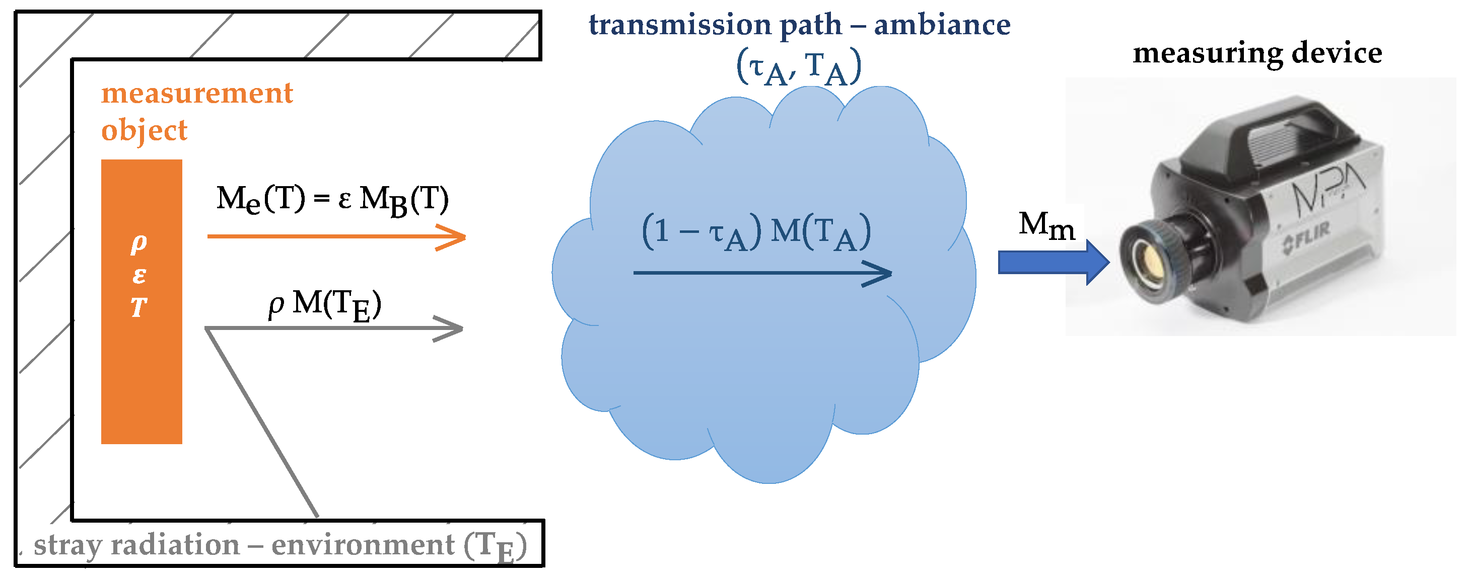
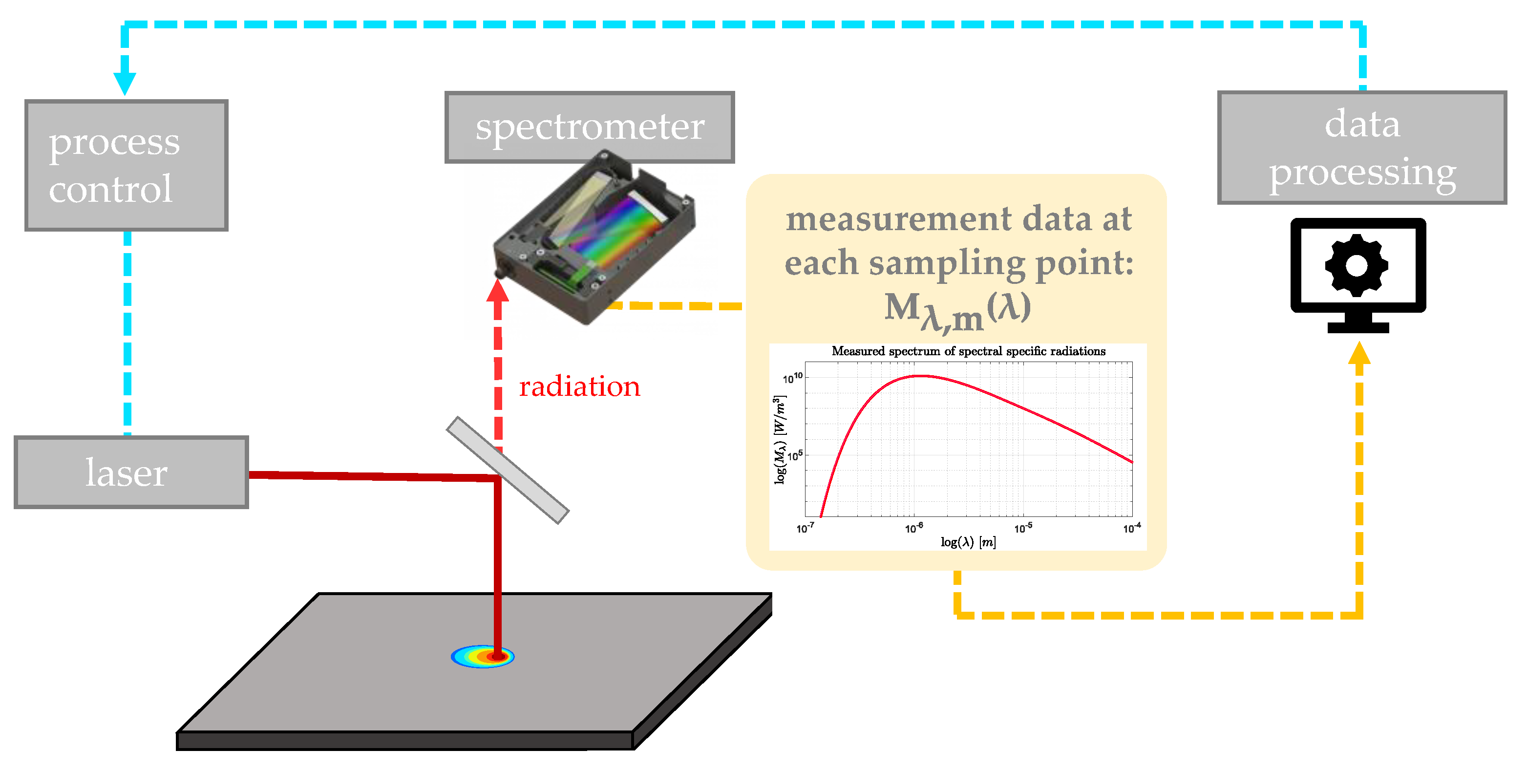
2.1. Measurement Approach

The proposed measurement setup uses a multispectral spectrometer to monitor the melt pool and its surroundings, including a part of the powder bed that is unaffected by the heat input. With that, the setup will measure the specific radiation in several spectral bands and give one intensity spectrum for each measuring period. This spectrum is then meant to be further processed in a way that allows for process control and quality assessment. The measurement approach is depicted in Figure 2. The internal design or optical channel of the spectrometer resembles a Czerny–Turner design. Here, the incoming light is first collimated by a spherical mirror. The collimated light is then diffracted by a grating. At the end, another spherical mirror focuses the diffracted light onto a one-dimensional linear detector array. More detailed descriptions of the Czerny–Turner Design can be found in [32,33,34]. This measurement approach differs from previous setups mainly in the size of the field of view and the processing of the measurement data. Until now, only thermal or multispectral cameras have been used to monitor an area of varying temperature distribution. Both allow a spatial representation of the temperature distribution directly from the measurement data.

The spectrometer’s line sensor provides a high temporal resolution of the emitted intensity spectrum. In order to use this information for process control and/or the quality assessment of the procedure itself, it needs to be processed further. This work aims to address the following questions in order to derive a suitable processing strategy for the measured data: Is it possible to gain spatial information about the temperature distribution in the measurement area if only spectral information is collected? Furthermore, would it be possible to differentiate between varying spatial distributions of temperature that might emit, by chance, similar radiation intensities in the detected wavelength spectrum? Moreover, could the spectrum of measured spectral intensities ${\mathrm{M}}_{\lambda ,\mathrm{m}}\left(\lambda \right)$ be represented with a linear superposition of several weighted Planck’s radiation spectra, i.e., the application of the Ritz method? To the author’s knowledge, the latter approach has not been used as a processing strategy for measured spectral radiation intensities. It would equal the following expression:

$${\mathrm{M}}_{\lambda ,\mathrm{m}}\left(\lambda \right)\approx {\mathrm{x}}_1{\mathrm{M}}_{\lambda ,\mathrm{B}}\left(\lambda ,{\mathrm{T}}_1\right)+{\mathrm{x}}_2{\mathrm{M}}_{\lambda ,\mathrm{B}}\left(\lambda ,{\mathrm{T}}_2\right)+\dots +{\mathrm{x}}_{\mathrm{i}}{\mathrm{M}}_{\lambda ,\mathrm{B}}\left(\lambda ,{\mathrm{T}}_{\mathrm{i}}\right)$$

(6)

The above questions are answered in this work from a theoretical (physical-mathematical) point of view. For this, the following assumptions are made: (a) ideal measurement conditions, i.e., no losses during the transmission, detection, or processing of the radiation intensity, (b) no stray radiation, (c) the monitored measurement object behaves like a black body, and (d) the radiation is detected for discrete wavelengths instead of spectral bands.

2.2. Theoretical Considerations

In order to better understand the relation between the emitted and detected spectral-specific radiation intensities of the measurement setup, the operating principle of a radiation quantum detector is further examined. Using a quantum detector, the energy of the incoming radiation, specifically the energy of each photon, is absorbed by the material of the semiconductor, causing a photoelectric current proportional to the radiation intensity. Thus, the connection between the spectral energy quantities and the spectral photon quantities is determined using the definition of spectrometric entities from the literature [12]:

$${\mathrm{M}}_{\lambda }=\frac{\mathrm{dM}}{\mathrm{d}\lambda }=\frac{{\mathrm{d}}^2\varphi }{\mathrm{d}\lambda \mathrm{d}{\mathrm{A}}_{\mathrm{e}}}=\frac{{\mathrm{d}}^3\mathrm{Q}}{\mathrm{d}\lambda \mathrm{d}{\mathrm{A}}_{\mathrm{e}} \mathrm{dt}}=\frac{{\mathrm{d}}^2{\mathrm{Q}}_{\lambda }}{\mathrm{d}{\mathrm{A}}_{\mathrm{e}} \mathrm{dt}}=\frac{{\mathrm{d}}^2}{\mathrm{d}{\mathrm{A}}_{\mathrm{e}} \mathrm{dt}}\left({\mathrm{W}}_{\mathrm{P},\lambda }·{\mathrm{N}}_{\mathrm{P},\lambda }\right)$$

(7)

where ${\mathrm{M}}_{\lambda }$ represents the radiation intensity that the quantum detector absorbs for a specific wavelength $\lambda$. The spectrometric entities $\varphi$, $\mathrm{Q}$, ${\mathrm{Q}}_{\lambda }$, ${\mathrm{W}}_{\mathrm{P},\lambda }$ and ${\mathrm{N}}_{\mathrm{P},\lambda }$ denote, respectively, the radiation power, the radiation energy, the spectral intensity of the radiation energy, the energy of a photon with wavelength $\lambda$, and the number of photons with wavelength $\lambda$. The parameter ${\mathrm{A}}_{\mathrm{e}}$ describes the emitting radiation surface. Next, Equation (7) is compared to Planck’s radiation law (Equation (2)), yielding the following expression:

$$\frac{{\mathrm{d}}^2}{\mathrm{d}{\mathrm{A}}_{\mathrm{e}} \mathrm{dt}}\left({\mathrm{W}}_{\mathrm{P},\lambda } · {\mathrm{N}}_{\mathrm{P},\lambda }\right)=\frac{{\mathrm{C}}_1}{{\lambda }^5 (\exp \left({\mathrm{C}}_2/\lambda \mathrm{T}\right)-1)}$$

$${\mathrm{W}}_{\mathrm{P},\lambda } · {\mathrm{N}}_{\mathrm{P},\lambda }=\int \int \frac{{\mathrm{C}}_1}{{\lambda }^5 (\exp \left({\mathrm{C}}_2/\lambda \mathrm{T}\right)-1)}\mathrm{d}{\mathrm{A}}_{\mathrm{e}} \mathrm{dt}$$

(8)

In general, it is $\mathrm{T}=\mathrm{f}(\mathrm{x},\mathrm{y},\mathrm{t})$. Here, a stationary temperature distribution during each measuring period $\Delta \mathrm{t}$ is assumed. This is valid if the melt pool dynamic is monitored in real-time, as described in [25]. Additionally, it is assumed that the sampling frequency does not change during the process and depends on the maximum scanning speed of the laser. Those assumptions lead to the following equation:

$${\mathrm{W}}_{\mathrm{P},\lambda } · {\mathrm{N}}_{\mathrm{P},\lambda }=\int \frac{{\mathrm{C}}_1}{{\lambda }^5 (\exp \left({\mathrm{C}}_2/\lambda \mathrm{T}(\mathrm{x},\mathrm{y})\right)-1)}\Delta \mathrm{t} \mathrm{d}{\mathrm{A}}_{\mathrm{e}}$$

(9)

The measurement area ${\mathrm{A}}_{\mathrm{e}}$ can be represented by an assemblage of k subareas ${\mathrm{A}}_{\mathrm{i}}$. Now, if the subareas are sufficiently small, yielding a constant temperature ${\mathrm{T}}_{\mathrm{i}}$, Equation (9) can be converted into:

$$\frac{{\mathrm{W}}_{\mathrm{P},\lambda } · {\mathrm{N}}_{\mathrm{P},\lambda }}{ \Delta \mathrm{t}}=\sum _{\mathrm{i}=1}^{\mathrm{k}}\frac{{\mathrm{C}}_1}{{\lambda }^5 (\exp \left({\mathrm{C}}_2/\lambda { \mathrm{T}}_{\mathrm{i}}\right)-1)}{\mathrm{A}}_{\mathrm{i}}$$

(10)

Considering normalized subareas with ${\mathrm{a}}_{\mathrm{i}}={\mathrm{A}}_{\mathrm{i}}/{\mathrm{A}}_{\mathrm{e}}$, yields:

$$\frac{{\mathrm{W}}_{\mathrm{P},\lambda } · {\mathrm{N}}_{\mathrm{P},\lambda }}{{\mathrm{A}}_{\mathrm{e}} \Delta \mathrm{t}}=\sum _{\mathrm{i}=1}^{\mathrm{k}}\frac{{\mathrm{C}}_1}{{\lambda }^5 (\exp \left({\mathrm{C}}_2/\lambda { \mathrm{T}}_{\mathrm{i}}\right)-1)}{\mathrm{a}}_{\mathrm{i}}={\mathrm{a}}_1{\mathrm{M}}_{\lambda ,\mathrm{B}}\left(\lambda ,{\mathrm{T}}_1\right)+\dots +{\mathrm{a}}_{\mathrm{k}}{\mathrm{M}}_{\lambda ,\mathrm{B}}\left(\lambda ,{\mathrm{T}}_{\mathrm{k}}\right)$$

(11)

This means, the detected spectral radiation energy emitted by the measurement area during each measuring period equals the areal average of all intensity spectra emitted by subareas of constant temperature inside the FoV. The right-hand side of Equation (11) resembles a linear superposition where each summand is weighted with its respective normalized subarea. With this, a physical foundation of the problem statement is found, since considering $\mathrm{n} \ll \mathrm{k}$ areas in Equation (11) leads back to Equation (6):

$${\mathrm{M}}_{\lambda ,\mathrm{m}}\left(\lambda \right)={\mathrm{a}}_1{\mathrm{M}}_{\lambda ,\mathrm{B}}\left(\lambda ,{\mathrm{T}}_1\right)+\dots +{\mathrm{a}}_{\mathrm{k}}{\mathrm{M}}_{\lambda ,\mathrm{B}}\left(\lambda ,{\mathrm{T}}_{\mathrm{k}}\right)$$

$$\approx {\mathrm{x}}_1{\mathrm{M}}_{\lambda ,\mathrm{B}}\left(\lambda ,{\mathrm{T}}_1\right)+\dots +{\mathrm{x}}_{\mathrm{n}}{\mathrm{M}}_{\lambda ,\mathrm{B}}\left(\lambda ,{\mathrm{T}}_{\mathrm{n}}\right)={\widehat{\mathrm{M}}}_{\lambda }\left(\lambda \right)$$

(12)

The interpretation of the weighting factors ${\mathrm{x}}_{\mathrm{i}}$ from Equation (6) as normalized areas of constant temperature ${\mathrm{T}}_{\mathrm{i}}$ imposes the following conditions:

$${\sum }_{\mathrm{i}=1}^{\mathrm{n}}{\mathrm{x}}_{\mathrm{i}}=1$$

(13)

$$0\le {\mathrm{x}}_{\mathrm{i}}\le 1$$

(14)

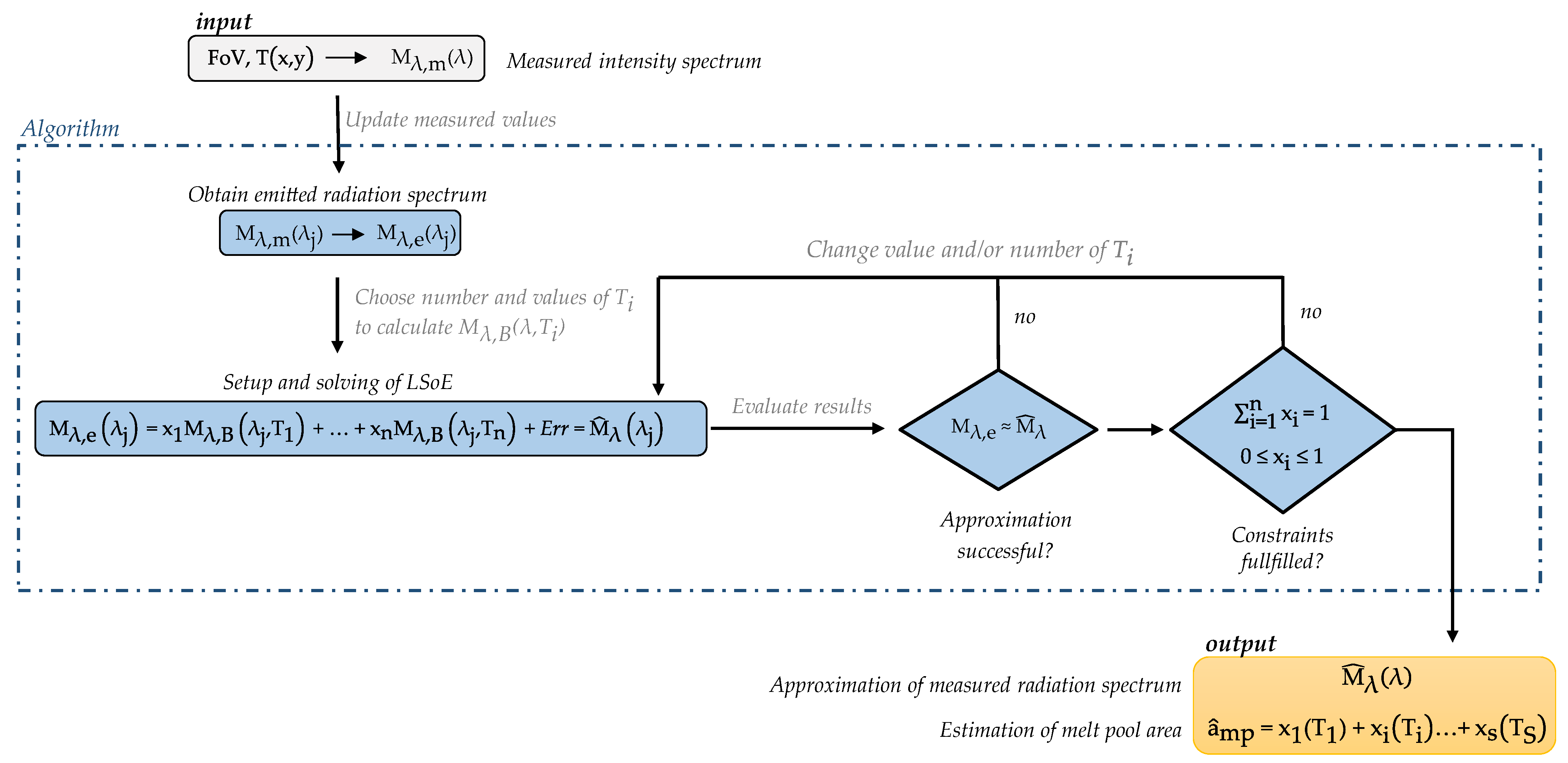
2.3. Methodology of Computational Studies

Computational studies represent the processing of the measurement data in Figure 2. The proposed strategy is to approximate the emitted spectrum of radiation intensity ${\mathrm{M}}_{\lambda ,\mathrm{e}}\left(\lambda \right)$ with a linear superposition of n radiation spectra ${\mathrm{M}}_{\lambda ,\mathrm{B}}\left(\lambda ,{\mathrm{T}}_{\mathrm{i}}\right)$—calculated after Planck’s law for the temperatures ${\mathrm{T}}_{\mathrm{i}}$ as described in Equation (2). To obtain suitable weighting factors ${\mathrm{x}}_{\mathrm{i}}$, the approximated spectrum ${\widehat{\mathrm{M}}}_{\lambda }\left(\lambda \right)$ must resemble the spectrum ${\mathrm{M}}_{\lambda ,\mathrm{e}}\left(\lambda \right)$ emitted by the measurement area at certain wavelengths ${\lambda }_{\mathrm{j}}$ with a sufficiently small error $\mathrm{Err}$. Those wavelengths ${\lambda }_{\mathrm{j}}$ correspond to the detectable wavelengths from the measurement setup in Figure 2. Due to the assumption listed in Section 2.1, the emitted spectral radiation intensities equal the measured spectral intensities.

$${\mathrm{M}}_{\lambda ,\mathrm{e}}\left({\lambda }_{\mathrm{j}}\right)={\mathrm{M}}_{\lambda ,\mathrm{m}}\left({\lambda }_{\mathrm{j}}\right)={\widehat{\mathrm{M}}}_{\lambda }\left({\lambda }_{\mathrm{j}}\right)+\mathrm{Err}$$

(15)

Furthermore, it is intended that each weighting factor ${\mathrm{x}}_{\mathrm{i}}$ can be interpreted as the surface area of a subdomain of constant temperature within the measurement field. This would allow estimating the melt pool area ${\widehat{\mathrm{a}}}_{\mathrm{mp}}$ by adding all weighting factors that represent a subdomain with a temperature equal to or greater than the solidification temperature ${\mathrm{T}}_{\mathrm{S}}$ of the processed material. This means that the proposed processing strategy for the measured data would generate a physically interpretable output entity. This entity could be further used for process control or quality assessment.

$${\widehat{\mathrm{a}}}_{\mathrm{mp}}={\mathrm{x}}_1\left({\mathrm{T}}_1\right)+\dots +{\mathrm{x}}_{\mathrm{i}}\left({\mathrm{T}}_{\mathrm{i}}\right)+\dots +{\mathrm{x}}_{\mathrm{S}}\left({\mathrm{T}}_{\mathrm{S}}\right)$$

(16)

The analytical representation of the considered measurement setup, given in Equation (15), is transferred into an algorithm to numerically obtain the approximation of the measured intensity spectrum ${\widehat{\mathrm{M}}}_{\lambda }\left(\lambda \right)$ for different test cases, i.e., temperature distributions in the measurement field. For this, a linear system of equations (LSoE) based on Equation (15) is defined and solved for a user-defined number of superimposed Planck’s radiation spectra. Afterwards, the success of the approximation and the fulfillment of Equation (13) and Inequality (14) are checked. A graphical representation of the described methodology is given in Figure 3. The illustrated process is repeated for each measuring period $\Delta \mathrm{t}$.

In this work, the spectral response range of the radiation detectors is assumed to be as follows:

$$500 \mathrm{nm}\le \lambda \le 5 \mu \mathrm{m}$$

(17)

For the setup of the LSoE, the values of the temperatures ${\mathrm{T}}_{\mathrm{i}}$ required to calculate Planck’s radiation spectra ${\mathrm{M}}_{\lambda ,\mathrm{B}}\left(\lambda ,{\mathrm{T}}_{\mathrm{i}}\right)$ must be chosen as a next step. It seems reasonable to select only values ranging between the minimum and maximum temperature that can possibly occur during the monitored PBF-LB/M process. Here, the minimum could be as high as the ambient temperature, and the maximum could be derived from the process parameters (laser power, scanning speed), and the material properties, either with an analytical function or a numerical simulation. In this work, a preheated building chamber is assumed for all numerical analyses, and the maximum temperature is chosen to be slightly less than the boiling temperature of 3153 K for SS 316L (after [29]).

Table 1. Important temperature values used in all investigations.

${\mathbf{T}}_{\mathbf{min}}\left[\mathbf{K}\right]$	${\mathbf{T}}_{\mathbf{S}}\left[\mathbf{K}\right]$	${\mathbf{T}}_{\mathbf{m}\mathbf{ax}}\left[\mathbf{K}\right]$
323.15	1660 [23]	3100

summarizes the most important temperature values considered in the investigated test cases, with ${\mathrm{T}}_{\mathrm{S}}$ denoting the solidification temperature.

The values and/or number of the temperatures ${\mathrm{T}}_{\mathrm{i}}$ considered in the LSoE are changed iteratively until the error $\mathrm{Err}$, see Equation (15), is small enough and the constraints for the weighting factors, see Equation (13) and Inequality (14), are fulfilled. If the error $\mathrm{Err}$ is small enough, the approximation is considered successful. In the following computational studies, the success of the approximation is evaluated according to the following criteria:

$$\begin{array}{l}{\mathrm{c}}_1=\frac{1}{\mathrm{w}}{\sum }_{\mathrm{j}}{\left(\frac{{\mathrm{M}}_{\lambda ,\mathrm{e}}\left({\lambda }_{\mathrm{j}}\right)-{\widehat{\mathrm{M}}}_{\lambda }\left({\lambda }_{\mathrm{j}}\right)}{{\mathrm{M}}_{\lambda ,\mathrm{e},\max }}\right)}^2\\ {\mathrm{c}}_2=\frac{\left|{\mathrm{M}}_{\lambda ,\mathrm{e},\max }-{\widehat{\mathrm{M}}}_{\lambda ,\max }\right|}{{\mathrm{M}}_{\lambda ,\mathrm{e},\max }}\\ {\mathrm{c}}_3=\frac{\left|\lambda \left({\mathrm{M}}_{\lambda ,\mathrm{e},\max }\right)-\lambda \left({\widehat{\mathrm{M}}}_{\lambda ,\max }\right)\right|}{\lambda \left({\mathrm{M}}_{\lambda ,\mathrm{e},\max }\right)}\end{array}\}\le 0.5\%$$

(18)

With ${\mathrm{c}}_1$ representing the mean-squared error between the reconstructed and the emitted spectral-specific radiation, respectively, normalized with the highest emitted spectral-specific radiation ${\mathrm{M}}_{\lambda ,\mathrm{e},\max }$. The number of considered wavelengths in the measurement range is denoted by the parameter w. The second and third criteria correspond to the relative deviation between the maximum intensities and their associated wavelengths.

2.4. Surrogate Reference Data

Since the investigation of the spectroscopic measurement setup in Figure 2 is carried out under several simplifications, calculated values of ${\mathrm{M}}_{\lambda ,\mathrm{m}}\left({\lambda }_{\mathrm{j}}\right)$ are used as surrogate measurement values for the computational studies. To obtain these values, the size of the field of view or measurement area (${\mathrm{A}}_{\mathrm{e}}$ or ${\mathrm{A}}_{\mathrm{FoV}}$) must first be defined. Then, an analytical formulation of the temperature distribution, denoted as ${\mathrm{T}}_{\mathrm{FoV}}(\mathrm{x},\mathrm{y})$, is chosen, which specifies the temperature at each point of the FoV. Afterwards, the FoV is discretized into smaller areas of equal size $\Delta {\mathrm{A}}_{\mathrm{e}}$. Note that this discretization inherently includes the discretization of the temperature distribution. For each subarea $\Delta {\mathrm{A}}_{\mathrm{e}}$ the spectral radiation intensities ${\mathrm{M}}_{\lambda ,\mathrm{m}}\left(\lambda \right)$ are calculated based on Equation (11). The spatial discretization is refined until the mean squared deviation of the spectral distribution of the surrogate measurement spectrum ${\mathrm{M}}_{\lambda ,\mathrm{m}}\left(\lambda \right)$ between two discretization levels is less than 0.5%. This spectrum is then used as input to the algorithm. Further, the surrogate size of the melt pool area can be determined by adding up all subareas $\Delta {\mathrm{A}}_{\mathrm{e}}$ with an assigned temperature equal to or greater than the solidification temperature. This value is referred to as the reference melt pool area ${\mathrm{a}}_{\mathrm{mp},\mathrm{FoV}}$ in the following.

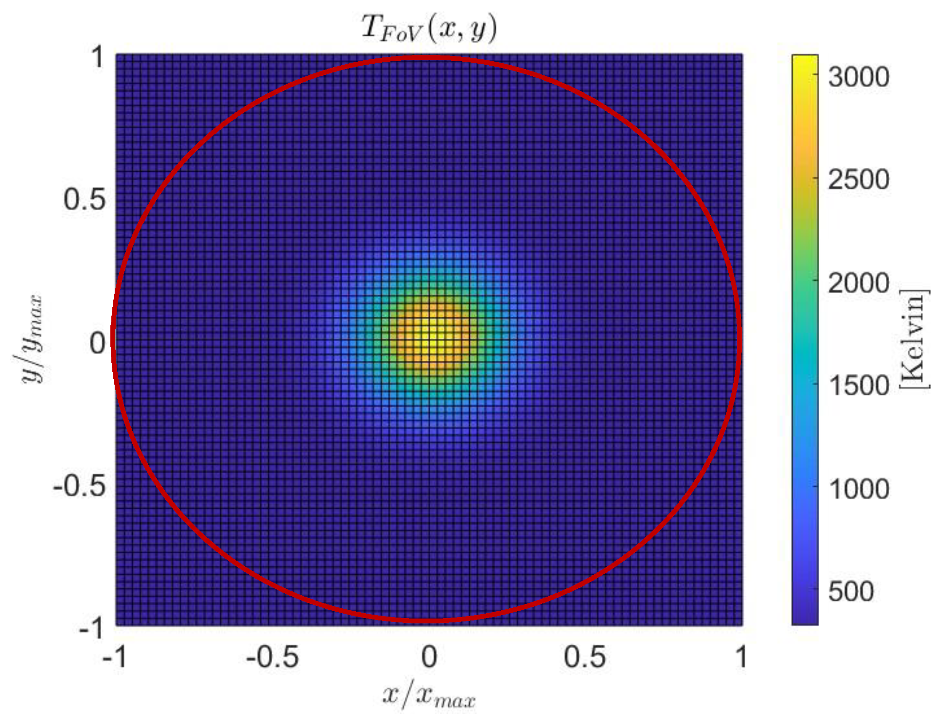
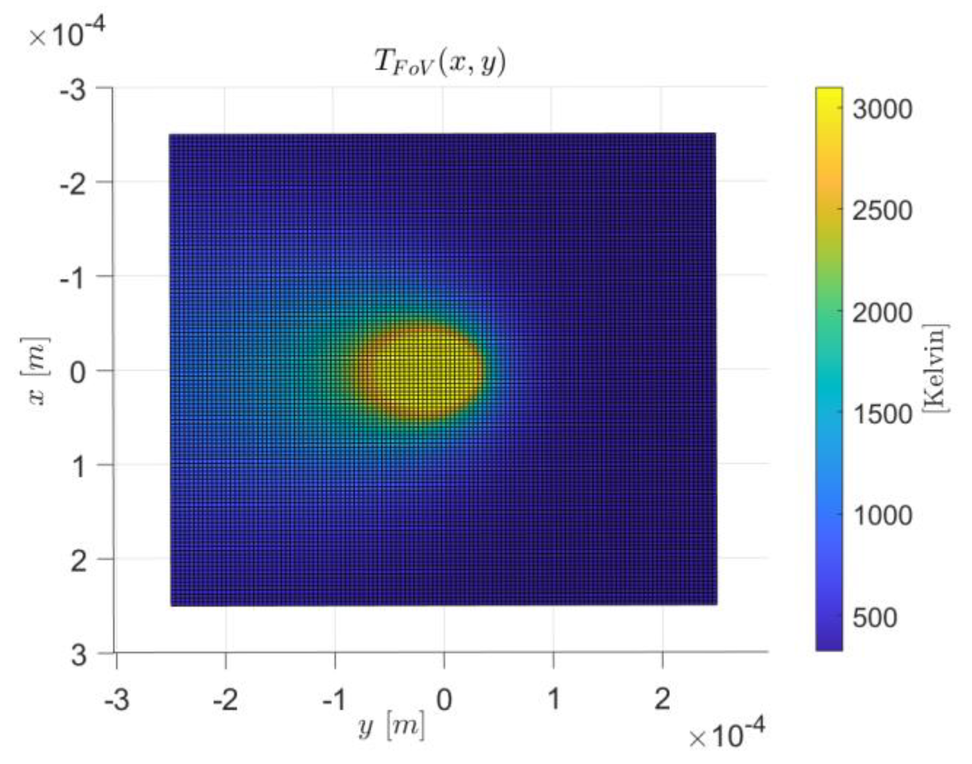
3. Computational Studies

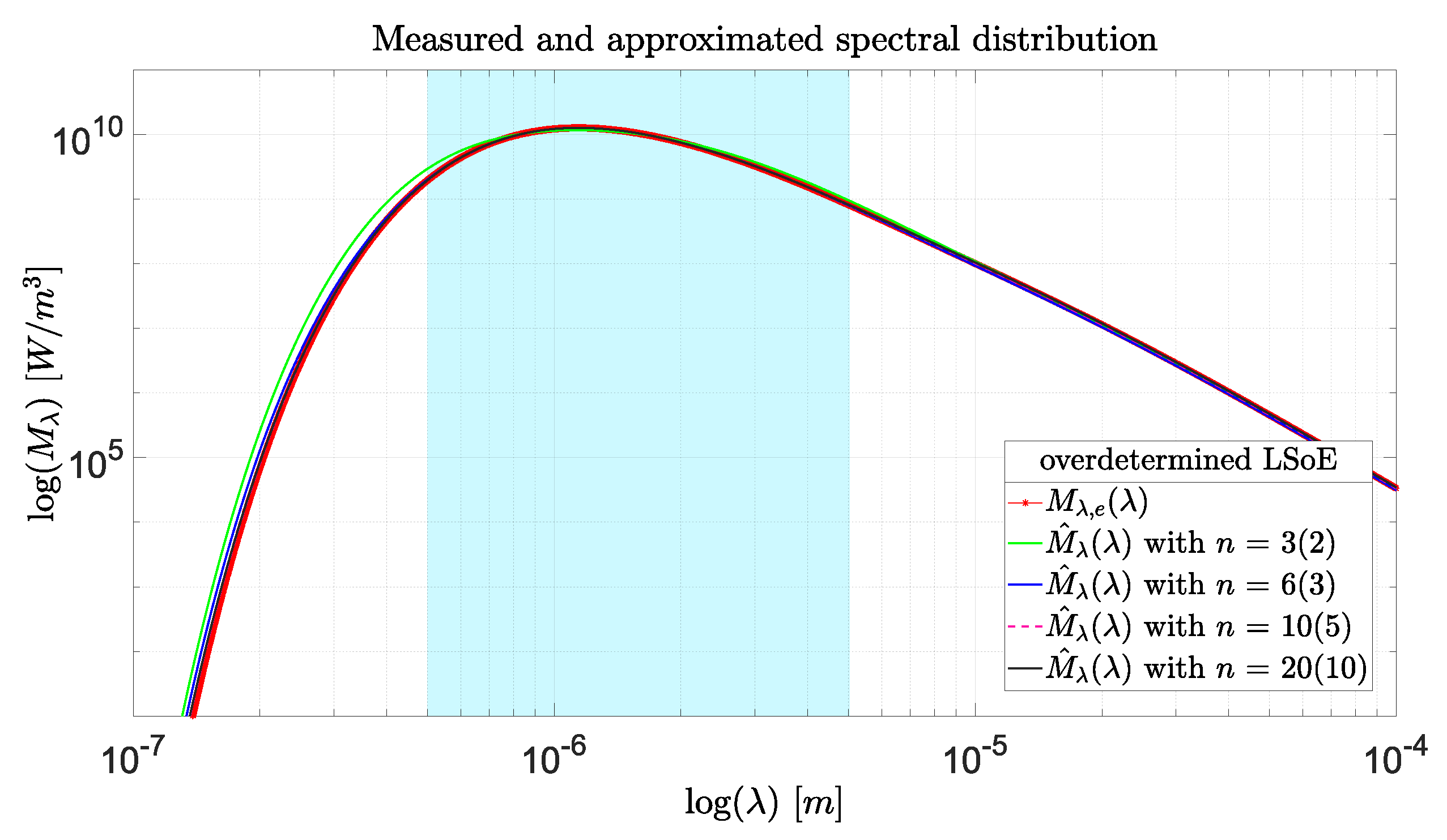
3.1. Load Case of a Pulse Laser

For the first investigation, a temperature profile resulting from the energy input of a pulse laser is chosen. The temperature distribution complies with a bell-shaped curve where the peak of the curve equals the highest temperature occurring in the FoV, that is, at the center of the laser beam. The analytical representation is given in Equation (19) and is based on a Gaussian normal distribution.

$${\mathrm{T}}_{\mathrm{FoV}}\left(\mathrm{x},\mathrm{y}\right)=\mu {\mathrm{e}}^{-\sigma \sqrt{{\mathrm{x}}^2+{\mathrm{y}}^2}}+{\mathrm{T}}_{\min }$$

$$\mu ={\mathrm{T}}_{\max }-{\mathrm{T}}_{\min }, \sigma =-\log ({(\mathrm{T}}_{\mathrm{S}}-{\mathrm{T}}_{\min })/({\mathrm{T}}_{\max }-{\mathrm{T}}_{\min }\left)\right)/{\mathrm{r}}_{\mathrm{mp}}^2$$

(19)

The melt pool is defined as a circular area with the same dimensions as the incoming laser beam. The radius of the latter is chosen as: ${\mathrm{r}}_{\mathrm{mp}}=50 \mu \mathrm{m}$. The measurement area is defined as a circular area with a radius of ${\mathrm{r}}_{\mathrm{FoV}}=250 \mu \mathrm{m}$. The corresponding temperature distribution is depicted in Figure 4. The spatial discretization is determined in analogy to Section 2.4.

As one of the desired results of solving the LSoE with the presented methodology is to approximate the melt pool size, the physical interpretability of the weighting factors ${\mathrm{x}}_{\mathrm{i}}$ as areas of surface subdomains must be maintained. Therefore, the first constraint given in Equation (13) is included in the LSoE, yielding the analytical expression given in Equation (20) to solve. Furthermore, to ensure that all weighting factors ${\mathrm{x}}_{\mathrm{i}}$ lie within the range of zero to one, Inequality (14) needs to be considered while solving the LSoE. This is possible by solving Equation (20) as an overdetermined LSoE with $\mathrm{w}>\mathrm{n}+1$ and including Inequality (14) as an additional constraint. For this, the solver for constrained linear least-squares problems “lsqlin” in MATLAB R2023a is used. This solver allows the definition of a lower and an upper boundary for the variable to be solved. With this, Inequality (14) can be considered. Furthermore, the LSoE is pre-conditioned in order to guarantee the fulfillment of the first row, i.e., the sum of all weighting factors equals one.

$$\begin{gathered} \left[\begin{array}{ccc}\begin{array}{c}1\\ {\mathrm{M}}_{\lambda ,\mathrm{B}}\left({\lambda }_1,{\mathrm{T}}_1\right)\end{array}& \cdots & \begin{array}{c}1\\ {\mathrm{M}}_{\lambda ,\mathrm{B}}\left({\lambda }_1,{\mathrm{T}}_{\mathrm{n}}\right)\end{array}\\ ⋮& \ddots & ⋮\\ {\mathrm{M}}_{\lambda ,\mathrm{B}}\left({\lambda }_{\mathrm{w}},{\mathrm{T}}_1\right)& \cdots & {\mathrm{M}}_{\lambda ,\mathrm{B}}\left({\lambda }_{\mathrm{w}},{\mathrm{T}}_{\mathrm{n}}\right)\end{array}\right]\left[\begin{array}{c}\begin{array}{c}{\mathrm{x}}_1\\ {\mathrm{x}}_2\end{array}\\ ⋮\\ {\mathrm{x}}_{\mathrm{n}}\end{array}\right]=\left[\begin{array}{c}\begin{array}{c}1\\ {\mathrm{M}}_{\lambda ,\mathrm{e}}\left({\lambda }_1\right)\end{array}\\ ⋮\\ {\mathrm{M}}_{\lambda ,\mathrm{e}}\left({\lambda }_{\mathrm{w}}\right)\end{array}\right] \\ ⟺\hspace{1em}\hspace{1em}\hspace{1em}\hspace{1em}\mathbf{A}\hspace{1em}\hspace{1em}\hspace{1em}\hspace{1em}\hspace{1em}\hspace{1em}\hspace{1em}\mathbf{x}\hspace{1em}\hspace{1em}=\hspace{1em}\hspace{1em}\mathbf{b} \end{gathered}$$

(20)

For the investigation of the load case, the LSoE is set up using n = 3(2), n = 6(3), n = 10(5), and n = 20(10) temperatures or Planck’s spectra to reconstruct the measured intensity spectrum. Here, the number of temperature values that are above the solidification temperature is given in parentheses. For example, n = 10(5) means that five temperature values are defined as ${\mathrm{T}}_{\mathrm{i}}\ge {\mathrm{T}}_{\mathrm{S}}$. In specific, the considered temperature values ${\mathrm{T}}_{\mathrm{i}}$ are chosen with a constant temperature increment ${\Delta \mathrm{T}}_1$ ranging from the maximum to the solidification temperature. The remaining part of the temperature is chosen with a constant temperature increment ${\Delta \mathrm{T}}_2$ from the solidification to the minimum temperature in the building chamber. The corresponding results using $\mathrm{w}=\mathrm{n}+20$ wavelengths are showcased in Figure 5. The outcome reveals that all criteria and constraints from the methodology given in Figure 3 are satisfied except in the case of n = 3, for which the criteria ${\mathrm{c}}_2=7.6\%$ and ${\mathrm{c}}_3=0.97\%$ are above the threshold of $0.5\%$.

Defining the LSoE as overdetermined and solving it accordingly enables the approximation of the measured spectral distribution with any number larger than three of Planck’s spectra while ensuring the physical interpretability of the weighting factors as normalized areas of constant temperature in the FoV of the spectrometer. A comparison between the approximated melt pool area ${\widehat{\mathrm{a}}}_{\mathrm{mp}}$ and the reference melt pool area ${\mathrm{a}}_{\mathrm{mp},\mathrm{FoV}}$ is determined with

$$∆{\mathrm{a}}_{\mathrm{mp}}=({\mathrm{a}}_{\mathrm{mp},\mathrm{FoV}}-{\widehat{\mathrm{a}}}_{\mathrm{mp}})/{\mathrm{a}}_{\mathrm{mp},\mathrm{FoV}}$$

(21)

$${\mathrm{a}}_{\mathrm{mp},\mathrm{FoV}}=0.04$$

(22)

The methodology yields for n = {6, 20} very good results with $∆{\mathrm{a}}_{\mathrm{mp}}=\left\{4.3, 2.9\right\}\%$, respectively. For n = 10, the deviation was larger, with $∆{\mathrm{a}}_{\mathrm{mp}}=$ 14.7%.

3.2. Load Case of a Moving Laser

In this subsection, the proposed methodology and the findings from the previous section are applied to investigate a different temperature field in order to evaluate the applicability of the methodology. The temperature distribution resembles a moving laser beam and is calculated after [36] with the following equation:

$${\mathrm{T}}_{\mathrm{FoV}}\left(\mathrm{x},\mathrm{y}\right)={\mathrm{T}}_{\min }+\frac{{\mathrm{P}}_0^{\prime }}{4 \pi \mathrm{K} \sqrt{{\mathrm{x}}^2+{\mathrm{y}}^2}}\exp \left(-{\mathrm{v}}_{\mathrm{laser}}(\sqrt{{\mathrm{x}}^2+{\mathrm{y}}^2 }+\mathrm{x}/2 \mathsf{\kappa }\right)$$

(23)

This represents the analytical solution for a point heat source in uniform motion on a semi-infinite plane. It allows the inclusion of material properties such as thermal diffusivity $\mathsf{\kappa }$ and thermal conductivity $\mathrm{K}$ and process parameters like the scanning speed of the laser ${\mathrm{v}}_{\mathrm{laser}}$ and the laser power ${\mathrm{P}}_0^{\prime }$ of the point source. Technically, Equation (23) is only valid up to the melting temperature of the considered material [36]. However, it is used here nonetheless to describe the whole temperature distribution in the measurement area, since it is assumed to sufficiently resemble real circumstances. Here, the FoV of the spectrometer is defined as a square area with an edge length of $2{\mathrm{r}}_{\mathrm{FoV}}=500 \mu \mathrm{m}$. The spatial discretization is determined in analogy to Section 2.4. Figure 6 displays the investigated temperature distribution. The setting of the algorithm, i.e., the values of n, w, and ${\mathrm{T}}_{\mathrm{i}}$, used for the approximation of the emitted spectral intensity distribution and the melt pool size, is the same as in Section 3.1. Considering $\mathrm{w}=\mathrm{n}+20$ wavelengths, an overdetermined LSoE is solved. For all but one parameter settings, i.e., n = {6, 10, 20}, the emitted spectral distribution is approximated successfully, and the weighting factor constraints in Equation (13) and Inequality (14) are satisfied. For the case of n = 3, the approximation is not considered successful since the values of ${\mathrm{c}}_2=1.9\%$ and ${\mathrm{c}}_3=1.4\%$ are above the threshold of 0.5%.

The numerical estimates of the normalized melt pool area ${\widehat{\mathrm{a}}}_{\mathrm{mp}}$ are summarized in

Table 2. Comparison of the reference melt pool area with the approximated melt pool area gained by solving an overdetermined LSoE.

${\mathbf{a}}_{\mathbf{mp},\mathbf{FoV}}$	n	w	${\widehat{\mathbf{a}}}_{\mathbf{mp}}$	$∆{\mathbf{a}}_{\mathbf{mp}}[\%]$
0.0689	6(3)	26	0.0852	−23.055
	10(5)	30	0.0804	−15.3055
	20(10)	40	0.0740	−5.1974

and compared to the reference melt pool area ${\mathrm{a}}_{\mathrm{mp},\mathrm{FoV}}$. The deviation of the melt pool area $∆{\mathrm{a}}_{\mathrm{mp}}$, calculated with Equation (21), is additionally listed. For the investigated parameter settings, the size of the melt pool area is overestimated. Further, it seems that the overestimation decreases, the more Planck’s spectra are linearly superimposed to approximate the measured intensity spectrum.

Next, the influence of increasing the size of the LSoE by considering more wavelengths, e.g., up to 320, is analyzed. It yields a very good approximation of the measured spectral radiation intensities with a higher number of wavelengths. Additionally, the deviation of the melt pool area is reduced. For example, it is reduced down to $∆{\mathrm{a}}_{\mathrm{mp}}=-2.46\%$ for the test case of n = 20. The success of the melt pool approximation varies depending on the number of temperature values greater than the solidification temperature. Exemplary results for approximating the emitted intensity spectrum for n = 20 Planck’s spectra and w = 40 wavelengths are given in part (a) of

Table 3. Comparison of the melt pool deviations resulting from varying the LSoE setting.

(a)			(b)
n	w	$∆{\mathbf{a}}_{\mathbf{mp}} [\%]$	n	w	$∆{\mathbf{a}}_{\mathbf{mp}} [\%]$
20(3)	40	20.48	50(25)	70	0.47
20(5)		−4.80	100(50)	120	1.09
20(8)		−1.73	200(100)	220	−2.88
20(15)		−19.12	500(250)	520	−7.70

. Increasing the number of temperature subdomains used to approximate the measured data does not necessarily lead to a better approximation of the reference melt pool area (refer to part (b) of Table 3). Both investigations show that the overestimation or underestimation of the size of the melt pool area depends on the setup of the LSoE.

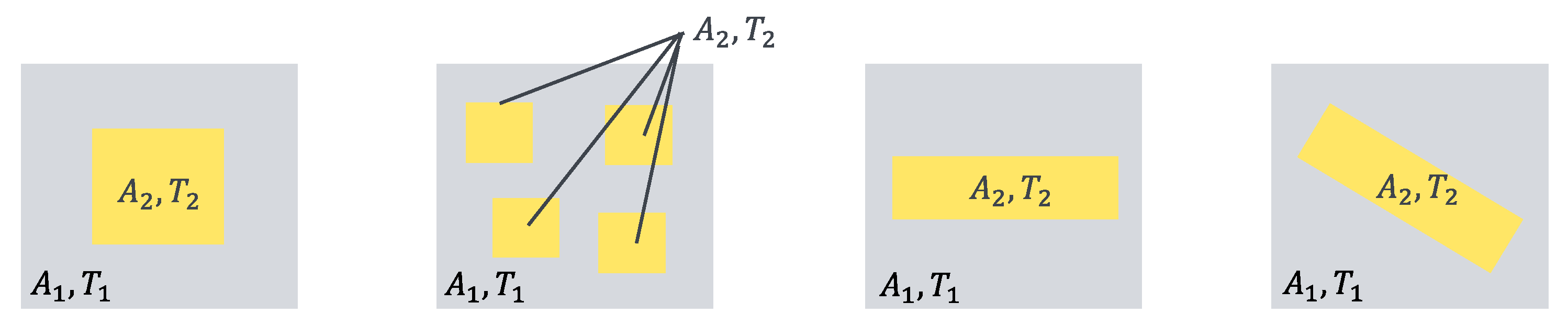
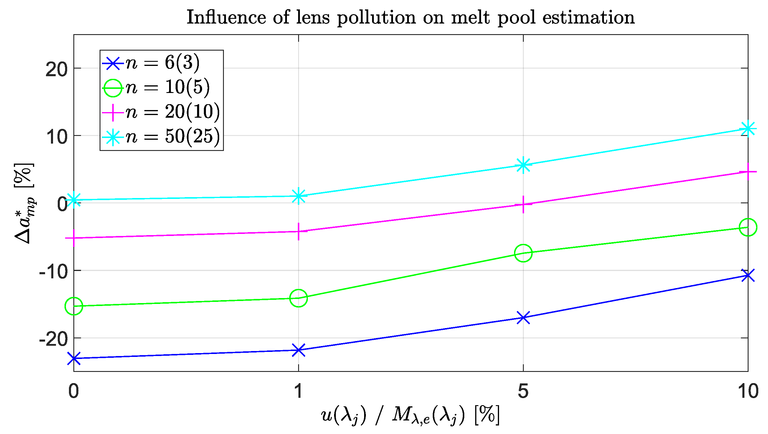
3.3. Numerical Modeling of Experimental Uncertainties

The assumptions made for an initial investigation of the problem statement and for testing the applicability of the methodology will not hold up once experimental data is fed into the algorithm. Therefore, this subsection intends to analyze the influence of some of the changes that are likely to be caused by a real physical measurement setup and real measurement circumstances on the outcome of the methodology. For this, the following test cases are examined: (a) mitigated radiation intensity due to a polluted lens, and (b) adjusted wavelength range based on the sensor sensitivity. Both test cases change the input to the algorithm in Figure 3. Analyzing the first test case of a polluted lens, the incoming radiation detected by the spectrometer is reduced. This decrease in spectral radiation intensity is represented in an adapted analytical representation of the measurement setup with the parameter $\mathrm{u}\left({\lambda }_{\mathrm{j}}\right)$ based on Equation (15), yielding:

$${\mathrm{M}}_{\lambda ,\mathrm{e}}^{\ast }\left({\lambda }_{\mathrm{j}}\right)={{\widehat{\mathrm{M}}}^{\ast }}_{\lambda }\left({\lambda }_{\mathrm{j}}\right)+\mathrm{Err}$$

$${\mathrm{M}}_{\lambda ,\mathrm{e}}\left({\lambda }_{\mathrm{j}}\right)-\mathrm{u}\left({\lambda }_{\mathrm{j}}\right)\approx {\mathrm{x}}_1^{\ast } {\mathrm{M}}_{\lambda ,\mathrm{B}}\left({\lambda }_{\mathrm{j}},{\mathrm{T}}_1\right)+\dots +{\mathrm{x}}_{\mathrm{n}}^{\ast } {\mathrm{M}}_{\lambda ,\mathrm{B}}\left({\lambda }_{\mathrm{j}},{\mathrm{T}}_{\mathrm{n}}\right)$$

(24)

Here, the asterisks are used to designate the LSoE used for investigating the effect of lens pollution. The corresponding analysis is conducted for the load case of the moving heat source with $\mathrm{n}=\{6,10,20,50\}$ and $\mathrm{w}=\mathrm{n}+20$. The pollution of the lens depends on the process itself (material, laser power, component volume, etc.) and is estimated in this work with: $\mathrm{u}\left({\lambda }_{\mathrm{j}}\right)=\left\{1\%, 5\%, 10\%\right\}{\mathrm{M}}_{\lambda ,\mathrm{e}}\left({\lambda }_{\mathrm{j}}\right)$. It shows that the algorithm approximates the mitigated spectral distribution very well. Moreover, the physical interpretability of the weighing factors is maintained for all three investigated pollution degrees. Figure 7 shows the influence on the melt pool approximation. Here, the melt pool area ${\widehat{\mathrm{a}}}_{\mathrm{mp}}^{\ast }={\mathrm{x}}_1^{\ast }+\dots +{\mathrm{x}}_{\mathrm{S}}^{\ast }$ is compared to ${\mathrm{a}}_{\mathrm{mp},\mathrm{FoV}}$ from Table 2.

It can be seen that the approximated melt pool area ${\widehat{\mathrm{a}}}_{\mathrm{mp}}^{\ast }$ decreases the more the lens is polluted and the measured radiation intensity is mitigated. Depending on the setting of the LSoE, this can reduce the deviation $\Delta {\mathrm{a}}_{\mathrm{mp}}^{\ast }$ regarding the reference melt pool area in the FoV. Additionally, the outcome of the numerical model using $\mathrm{n}=50$ Planck’s spectra for the reconstruction of the emitted spectral intensities is displayed. Here, the numerical model underestimates, in general, the size of the melt pool area.

For the second test case of an adjusted wavelength range based on the sensor sensitivity, the load case of a moving heat source with n = 20 is examined for two different sensor types. First, an InGaAs linear image sensor is assumed to be implemented in the spectroscopic measurement arrangement. This sensor is sensitive in the wavelength range of $900–1750\mathrm{nm}$ [35]. Further, it is assumed that, due to filters, only radiation in the range of $1100–1750\mathrm{nm}$ enters the spectrometer. Based on a potential spectral resolution of $2 \mathrm{nm}$ [37], leading to a total amount of $170$ spectral bands, the LSoE (Equation (20)) is solved for $\mathrm{w}=\left\{20, 170\right\}$ wavelengths. Second, the measurement arrangement is assumed to utilize InSb sensors, which are sensitive in the range of $3000–5000 \mathrm{nm}$ [38]. This analyzed setup detects radiation in $154$ wavelengths following [39]. Therefore, the LSoE is solved for $\mathrm{w}=\left\{20, 154\right\}$. The results are given in

Table 4. Outcome of solving the overdetermined LSoE considering two sensor sensitivity ranges.

n	w	$\lambda \left[\mathbf{nm}\right]$	Sensor Type	$∆{\mathbf{a}}_{\mathbf{mp}}[\%]$
20(10)	40	1100–1750	InGaAs	−3.58
	170			−5.31
	40	3000–5000	InSb	−5.19
	154			−8.82

. In all four setups, the emitted spectral radiation intensities are approximated well ($\left\{{\mathrm{c}}_1,{\mathrm{c}}_2,{\mathrm{c}}_3\right\}<0.5\%$) with the proposed methodology, and the constraint for the weighting factors is fulfilled. Moreover, the estimated melt pool area with respect to the reference has a deviation $\Delta {\widehat{\mathrm{a}}}_{\mathrm{mp}}$ of less than 10% in an acceptable range.

4. Discussion

The proposed methodology approximates the radiation intensity spectrum emitted by the measurement area, i.e., an area of varying temperature. This is achieved by superimposing the radiation intensity spectra emitted by a multitude of smaller areas of constant temperature. The sum of these smaller isothermal areas represents the FoV of the measurement setup. The number of subdomains applied to approximate the FoV is determined with the user defined number (n) and the values (${\mathrm{T}}_{\mathrm{i}}$) of the temperatures used to calculate the spectral intensities on the left-hand side of the LSoE. Further, a reasonable configuration of the LSoE allows an estimation of the melt pool area. However, neither the choice of an arbitrarily higher number of superimposed radiation spectra nor considering all detected spectral intensities guarantees a melt pool area approximation with a negligible deviation. Additionally, no information about the shape or the expansion in any direction of the subdomains can be derived with this method. For example, the temperature distributions shown in Figure 8 consist of two isothermal subdomains and emit the same amount of radiation intensity in the measured wavelength range. It would be possible to derive the size (${\mathrm{A}}_1, {\mathrm{A}}_2$) of each subdomain with the method examined in this work, but not the arrangement of each subdomain inside the measurement area. For this, further assumptions are necessary if they can be defined for the monitored process. This is one major difference to monitoring strategies utilizing thermal or multispectral cameras, as no graphical display of the temperature distribution in the FoV can be directly obtained.

Another difference is the small amount of data that needs to be stored and transmitted per measurement period. Offering the possibility of storing the processed measurement data over a longer period of time. For example, Hooper et al. [26] captured the melt pool characteristics at 100 kHz for a spatial resolution of 20 $\mu \mathrm{m}/\mathrm{pixel}$. With that, Hooper et al. sufficiently detected the melt pool dynamics but reached full storage after 3 s. In contrast, the computational investigation of the moving laser, using n = 10(5) Planck’s spectra and 30 wavelengths to set up the LSoE, took on average 0.15 s. The computations were performed on a Fujitsu computer, equipped with an Intel^® Core™ i5-8500 CPU and 32 GB of RAM. Note that the time needed for the processing of the measurement data can be decreased by optimizing the code as well as upgrading the hardware. To compare storage requirements and data transferability, for each measurement period only the weighting factors, e.g., 10, and the approximated melt pool area need to be stored. A total of 11 double precision floating-point numbers of 704 bits are required. Using Hooper’s settings with a sampling rate of 100 kHz [26], 26.4 MB of data would need to be saved after 3 s of the process. In addition, if only the approximate melt pool area is used for process control, 64 bits of data must be transferred.

The results of the different investigations conducted in Section 3 show that the outcome of the algorithm depends on the parameters of the LSoE, i.e., n, w, and ${\mathrm{T}}_{\mathrm{i}}$. Therefore, a preliminary study needs to be performed for each load case to identify the most appropriate model parameters before applying the proposed methodology in a manufacturing setup. Another important influence on the measured data is emissivity; see Equation (4). A possible approach to approximate the reduced radiation intensity due to the wavelength and temperature-dependent emissivity is to include the emissivity for each of the superimposed Planck’s radiation spectra. The expanded LSoE could be given by:

$${\mathrm{M}}_{\lambda ,\mathrm{m}}\left(\lambda \right)={\mathrm{a}}_1{\epsilon }_1\left(\lambda ,{\mathrm{T}}_1\right){\mathrm{M}}_{\lambda ,\mathrm{B}}\left(\lambda ,{\mathrm{T}}_1\right)+\dots +{\mathrm{a}}_{\mathrm{k}}{\epsilon }_{\mathrm{k}}\left(\lambda ,{\mathrm{T}}_{\mathrm{k}}\right) {\mathrm{M}}_{\lambda ,\mathrm{B}}\left(\lambda ,{\mathrm{T}}_{\mathrm{k}}\right)$$

$$\approx {\mathrm{x}}_1{\epsilon }_1\left(\lambda ,{\mathrm{T}}_1\right){ \mathrm{M}}_{\lambda ,\mathrm{B}}\left(\lambda ,{\mathrm{T}}_1\right)+\dots +{\mathrm{x}}_{\mathrm{n}}{\epsilon }_{\mathrm{n}}\left(\lambda ,{\mathrm{T}}_{\mathrm{n}}\right){ \mathrm{M}}_{\lambda ,\mathrm{B}}\left(\lambda ,{\mathrm{T}}_{\mathrm{n}}\right)={\widehat{\mathrm{M}}}_{\lambda }\left(\lambda \right)$$

(25)

This way, only a limited number of emissivity values matching the wavelengths and temperatures used to solve the linear system of equations need to be separately determined. Based on the reviewed literature regarding the monitoring of AM processes, only monitoring strategies using hyper- or multispectral cameras take the wavelength dependency of the emissivity for each monitored spot into account; see [29,30,31]. This means that for each spot, a constant temperature is assumed, which might resemble real circumstances if the spot is small enough. In other measurement setups, emissivity is assumed to be independent of wavelength and temperature. Therefore, only one value is determined and then applied to the entire intensity spectrum detected. Usually, the emissivity value corresponding to the solidification temperature is taken [6,21,22,23,24]. This assumption leads to a known error in the determination of absolute temperature values. The proposed measurement setup and data processing strategy offer the opportunity to include a fitting emissivity value for at least each considered Planck’s spectra on the right-hand side of the LSoE.

5. Conclusions and Outlook

In this work, a novel measurement approach to the powder bed fusion process was presented. In contrast to existing monitoring strategies, the presented setup approximates the size of the melt pool area with high temporal resolution but without generating a large amount of data. Thus, offering the opportunity of real-time process control and quality assessment with one process entity important to the performance of the manufacturing process. An initial analysis of the proposed measurement setup was conducted under several assumptions. It was shown that the measured radiation intensity spectrum can be approximated with a linear superposition of weighted Planck’s radiation spectra using the Ritz method. To the best of the author’s knowledge, this type of data processing has not previously been used in the context of production monitoring. Further, the theoretical considerations revealed that the weighting factors of the superimposed spectra can be interpreted as normalized areas of constant temperature if certain constraints are fulfilled, thus allowing an approximation of the melt pool area. The measurement approach was applied to different load cases resembling a pulse laser and a moving laser. For both load cases, the results using 3, 6, 5, and 10 Planck’s spectra for the reconstruction of the emitted intensity spectrum were compared. The mean squared error between the reconstructed and emitted spectra was less than 0.5% in all cases using more than three Planck’s spectra. For all test cases but the latter, the approximation of the melt pool area was calculated and compared to the reference melt pool area. For the load case of a pulse laser, the deviation between the approximated and reference melt pool area was 4.3%, 14.7%, and 2.9%. Showing a tendency to underestimate the melt pool area. For the second load case of a moving laser, the deviation was −23%, −15.3%, and −5.2% meaning that the size of the melt pool area was generally overestimated. It showed that the setting of the computational studies has a strong influence on the results.

In future works, the experimental implementation of the investigated spectroscopic arrangement to control the results of this work would be reasonable to pursue. In that context, factors like the proper determination of emissivity values or the influence of spatter, as well as partially higher radiation intensities due to oxide inclusions on the output of the numerical model, need further consideration. Moreover, the computational model could be adapted in order to consider the collection of radiation in spectral bands instead of discrete wavelengths. Also, studies need to be conducted to apply the information about the melt pool area and/or its temporal change as reasonable feedback to optimize process control.

References

1. Grasso, M.; Colosimo, B.M. Process defects and in situ monitoring methods in metal powder bed fusion: A review. Meas. Sci. Technol. 2017, 28, 44005. [Google Scholar] [CrossRef]
2. McCann, R.; Obeidi, M.A.; Hughes, C.; McCarthy, É.; Egan, D.S.; Vijayaraghavan, R.K.; Joshi, A.M.; Acinas Garzon, V.; Dowling, D.P.; McNally, P.J.; et al. In-situ sensing, process monitoring and machine control in Laser Powder Bed Fusion: A review. Addit. Manuf. 2021, 45, 102058. [Google Scholar] [CrossRef]
3. Mani, M.; Lane, B.; Donmez, A.; Feng, S.; Moylan, S.; Fesperman, R. Measurement Science Needs for Real-Time Control of Additive Manufacturing Powder Bed Fusion Processes; US Dept. of Commerce, National Institute of Standards and Technology: Gaithersburg, MD, USA, 2015. [Google Scholar] [CrossRef]
4. Thijs, L.; Verhaeghe, F.; Craeghs, T.; van Humbeeck, J.; Kruth, J.-P. A study of the microstructural evolution during selective laser melting of Ti–6Al–4V. Acta Mater. 2010, 58, 3303–3312. [Google Scholar] [CrossRef]
5. Lough, C.S.; Escano, L.I.; Qu, M.; Smith, C.C.; Landers, R.G.; Bristow, D.A.; Chen, L.; Kinzel, E.C. In-situ optical emission spectroscopy of selective laser melting. J. Manuf. Process. 2020, 53, 336–341. [Google Scholar] [CrossRef]
6. Doubenskaia, M.A.; Zhirnov, I.V.; Teleshevskiy, V.I.; Bertrand, P.; Smurov, I.Y. Determination of True Temperature in Selective Laser Melting of Metal Powder Using Infrared Camera. Mater. Sci. Forum 2015, 834, 93–102. [Google Scholar] [CrossRef]
7. Chen, L.; Yao, X.; Ng, N.; Moon, S.K. In-situ Melt Pool Monitoring of Laser Aided Additive Manufacturing using Infrared Thermal Imaging. In Proceedings of the IEEE International Conference on Industrial Engineering and Engineering Management, Kuala Lumpur, Malaysia, 7–10 December 2022; pp. 1478–1482. [Google Scholar] [CrossRef]
8. Ocylok, S.; Alexeev, E.; Mann, S.; Weisheit, A.; Wissenbach, K.; Kelbassa, I. Correlations of Melt Pool Geometry and Process Parameters During Laser Metal Deposition by Coaxial Process Monitoring. Phys. Procedia 2014, 56, 228–238. [Google Scholar] [CrossRef]
9. Schmidt, M.; Gorny, S.; Rüssmeier, N.; Partes, K. Investigation of Direct Metal Deposition Processes Using High-Resolution In-line Atomic Emission Spectroscopy. J. Therm. Spray Technol. 2023, 32, 586–598. [Google Scholar] [CrossRef]
10. Liu, Y.; Wang, L.; Brandt, M. An accurate and real-time melt pool dimension measurement method for laser direct metal deposition. Int. J. Adv. Manuf. Technol. 2021, 114, 2421–2432. [Google Scholar] [CrossRef]
11. Bernhard, F. Handbuch der Technischen Temperaturmessung; Springer: Berlin/Heidelberg, Germany, 2014. [Google Scholar]
12. Rahne, E. Thermografie: Theorie, Messtechnik, Praxis; 1. Auflage; Wiley-VCH GmbH: Weinheim, Germany, 2022; ISBN 352782071X. [Google Scholar]
13. Grujić, K. A Review of Thermal Spectral Imaging Methods for Monitoring High-Temperature Molten Material Streams. Sensors 2023, 23, 1130. [Google Scholar] [CrossRef]
14. Kulchin, Y.N.; Gribova, V.V.; Timchenko, V.A.; Basakin, A.A.; Nikiforov, P.A.; Yatsko, D.S.; Zhevtun, I.G.; Subbotin, E.P.; Nikitin, A.I. Melt Pool Temperature Control in Laser Additive Process. Bull. Russ. Acad. Sci. Phys. 2022, 86, S108–S113. [Google Scholar] [CrossRef]
15. Kolb, T.; Gebhardt, P.; Schmidt, O.; Tremel, J.; Schmidt, M. Melt pool monitoring for laser beam melting of metals: Assistance for material qualification for the stainless steel 1.4057. Procedia CIRP 2018, 74, 116–121. [Google Scholar] [CrossRef]
16. Krauss, H.; Zeugner, T.; Zaeh, M.F. Layerwise Monitoring of the Selective Laser Melting Process by Thermography. Phys. Procedia 2014, 56, 64–71. [Google Scholar] [CrossRef]
17. Rodriguez, E.; Mireles, J.; Terrazas, C.A.; Espalin, D.; Perez, M.A.; Wicker, R.B. Approximation of absolute surface temperature measurements of powder bed fusion additive manufacturing technology using in situ infrared thermography. Addit. Manuf. 2015, 5, 31–39. [Google Scholar] [CrossRef]
18. Scheuschner, N.; Altenburg, S.J.; Pignatelli, G.; Maierhofer, C.; Straße, A.; Gornushkin, I.B.; Gumenyuk, A. Vergleich der Messungen der Schmelzbadtemperatur bei der Additiven Fertigung von Metallen mittels IR-Spektroskopie und Thermografie. Tm Tech. Mess. 2021, 88, 626–632. [Google Scholar] [CrossRef]
19. Doubenskaia, M.; Smurov, I.; Grigoriev, S.; Pavlov, M.; Tikhonova, E. Optical Monitoring in Elaboration of Metal Matrix Composites by Direct Metal Deposition. Phys. Procedia 2012, 39, 767–775. [Google Scholar] [CrossRef]
20. Clijsters, S.; Craeghs, T.; Buls, S.; Kempen, K.; Kruth, J.-P. In situ quality control of the selective laser melting process using a high-speed, real-time melt pool monitoring system. Int. J. Adv. Manuf. Technol. 2014, 75, 1089–1101. [Google Scholar] [CrossRef]
21. Doubenskaia, M.; Pavlov, M.; Grigoriev, S.; Smurov, I. Definition of brightness temperature and restoration of true temperature in laser cladding using infrared camera. Surf. Coat. Technol. 2013, 220, 244–247. [Google Scholar] [CrossRef]
22. Altenburg, S.J.; Maierhofer, C.; Straße, A.; Gumenyuk, A. Comparison of MWIR thermography and high-speed NIR thermography in a laser metal deposition (LMD) process. In Proceedings of the 2018 International Conference on Quantitative InfraRed Thermography, Berlin, Germany, 25–29 June 2018. [Google Scholar]
23. Altenburg, S.J.; Straße, A.; Gumenyuk, A.; Maierhofer, C. In-situ monitoring of a laser metal deposition (LMD) process: Comparison of MWIR, SWIR and high-speed NIR thermography. Quant. InfraRed Thermogr. J. 2022, 19, 97–114. [Google Scholar] [CrossRef]
24. Lane, B.; Heigel, J.; Ricker, R.; Zhirnov, I.; Khromschenko, V.; Weaver, J.; Phan, T.; Stoudt, M.; Mekhontsev, S.; Levine, L. Measurements of melt pool geometry and cooling rates of individual laser traces on IN625 bare plates. Integr. Mater. Manuf. Innov. 2020, 9, 16–30. [Google Scholar] [CrossRef]
25. Berumen, S.; Bechmann, F.; Lindner, S.; Kruth, J.-P.; Craeghs, T. Quality control of laser- and powder bed-based Additive Manufacturing (AM) technologies. Phys. Procedia 2010, 5, 617–622. [Google Scholar] [CrossRef]
26. Hooper, P.A. Melt pool temperature and cooling rates in laser powder bed fusion. Addit. Manuf. 2018, 22, 548–559. [Google Scholar] [CrossRef]
27. Dörfert, R.; Tyralla, D. In-situ-Messung der Schmelzbadbreite beim pulverbettbasierten Laserstrahlschmelzen. In laf-Flashtalk Proceedings; BIAS—Bremer Institut für angewandte Strahltechnik GmbH: Bremen, Germany, 2020. [Google Scholar]
28. Lane, B.; Moylan, S.; Whitenton, E.; Ma, L. Thermographic Measurements of the Commercial Laser Powder Bed Fusion Process at NIST. Rapid Prototyp. J. 2016, 22, 778–787. [Google Scholar] [CrossRef]
29. Devesse, W.; de Baere, D.; Guillaume, P. High Resolution Temperature Measurement of Liquid Stainless Steel Using Hyperspectral Imaging. Sensors 2017, 17, 91. [Google Scholar] [CrossRef]
30. Gerdes, N.; Hoff, C.; Hermsdorf, J.; Kaierle, S.; Overmeyer, L. Hyperspectral imaging for prediction of surface roughness in laser powder bed fusion. Int. J. Adv. Manuf. Technol. 2021, 115, 1249–1258. [Google Scholar] [CrossRef]
31. Qu, D.-X.; Berry, J.; Calta, N.P.; Crumb, M.F.; Guss, G.; Matthews, M.J. Temperature Measurement of Laser-Irradiated Metals Using Hyperspectral Imaging. Phys. Rev. Appl. 2020, 14, 014031. [Google Scholar] [CrossRef]
32. O’Byrne, R.P.; Sergeyev, S.V.; Flavin, D.A.; Slattery, S.A.; Nikogosyan, D.N.; Jones, J.D.C. Anisotropic Fiber Bragg Gratings Inscribed by High-Intensity Femtosecond-UV Pulses: Manufacturing Technology and Strain Characterization for Sensing Applications. IEEE Sens. J. 2008, 8, 1256–1263. [Google Scholar] [CrossRef]
33. Shafer, A.B.; Megill, L.R.; Droppleman, L. Optimization of the Czerny–Turner Spectrometer. J. Opt. Soc. Am. 1964, 54, 879. [Google Scholar] [CrossRef]
34. Feng, Z.; Xia, G.; Lu, R.; Cai, X.; Cui, H.; Hu, M. High-Performance Ultra-Thin Spectrometer Optical Design Based on Coddington’s Equations. Sensors 2021, 21, 323. [Google Scholar] [CrossRef]
35. AVANTES. Optical Spectrometers Introduction—Must Read—Avantes. Available online: https://www.avantes.com/support/theoretical-background/introduction-to-spectrometers/ (accessed on 21 September 2023).
36. Angelastro, A.; Campanelli, S.L. An integrated analytical model for the forecasting of the molten pool dimensions in Selective Laser Melting. Laser Phys. 2022, 32, 26001. [Google Scholar] [CrossRef]
37. AVANTES. AvaSpec-NIR256/512-1.7-EVO—Avantes. Available online: https://www.avantes.com/products/spectrometers/nirline/avaspec-nir256-512-1-7-evo/ (accessed on 6 October 2023).
38. Infiniti Electro-Optics. InSb (Indium Antimonide). Available online: https://www.infinitioptics.com/glossary/insb (accessed on 21 September 2023).
39. Quantum Design, Inc. MWIR Spectral Camera Specim. Quantum Design. Available online: https://qd-europe.com/ro/en/product/mwir-spectral-camera/ (accessed on 6 October 2023).
Figure 1. Schematic visualization of the measurement section (picture of the measuring device in courtesy of MPA, University Stuttgart).
Jmmp 08 00073 g001
Figure 2. Illustration of the measurement approach analyzed in this work. The illustration of the spectrometer is from [35].
Jmmp 08 00073 g002
Figure 3. Methodology to approximate the measured intensity spectrum and the melt pool area.
Jmmp 08 00073 g003
Figure 4. Visualization of the investigated temperature distribution in the FoV (red circle).
Jmmp 08 00073 g004
Figure 5. Comparison of the surrogate measurement spectrum (red) M λ , e ( λ ) and its approximation M ^ λ ( λ ) , solving an overdetermined LSoE with T i ϵ   [ T max : T S : T min ] for i = 1:n and w = n + 20. The sensor’s spectral response range of the measurement setup is highlighted in blue.
Jmmp 08 00073 g005
Figure 6. Visualization of the investigated temperature distribution of a moving heat source.
Jmmp 08 00073 g006
Figure 7. Effects on the approximation of the melt pool area due to mitigated incoming radiation intensity.
Jmmp 08 00073 g007
Figure 8. Different explementary temperature distributions that would emit the same radiation spectrum.
Jmmp 08 00073 g008