Theoretical Assessment of the Environmental Impact of the Preheating Stage in Thermoplastic Composite Processing: A Step toward Sustainable Manufacturing

Abstract

Manufacturing processes have always played a pivotal role in the life cycle assessment of products, necessitating focused efforts to minimize their impact on the environment. Thermoplastic composite manufacturing is no exception to this concern. Within thermoplastic composite manufacturing, the preheating process stands out as one of the most energy-intensive stages, significantly affecting the environment. In this study, a theoretical analysis is conducted to compare three modes of preheating: conductive, radiative, and convective modes, considering their energy consumption and environmental impact. The analysis reveals the potential for substantial energy savings and emissions reduction through the selection of a proper preheating mode. Since the analysis used in this study is theoretical, it facilitates a parametric study of different modes of preheating to assess how process parameters impact the environment. Moreover, this study includes a comparison between emissions from material production and the preheating process, highlighting the substantial contribution of the preheating process to the overall product life cycle assessment.

1. Introduction

Even though many countries around the globe have been striving to pass legislation to move toward net-zero emissions to control global warming, there is no indication that this ambitious objective has been achieved [1]. To elaborate, emissions from the industry and energy production sectors have increased by 60% since the establishment of the United Nations Framework Convention on Climate Change in 1992 [2]. This trend has concerned researchers and industrial leaders to take action to reduce emissions. Manufacturing-related industries are among the largest contributors to harmful gas emissions, accounting for 30% of greenhouse gas emissions [3]. As such, developing sustainable manufacturing processes with reduced environmental impacts is extremely beneficial to address the concerning trend in industrial emissions [4]. Per the US Department of Commerce [5], sustainable manufacturing is “the creation of manufactured products that use processes that are nonpolluting, conserve energy and natural resources, and are economically sound and safe for employees, communities, and consumers”. One of the most effective ways in this direction is to integrate environmental impact indicators into the design process of products and their associated manufacturing processes. This strategy is referred to as Design For Environment (DfE), which can be implemented through life cycle assessment methods [6].

Life Cycle Assessment (LCA) is a technique to quantitatively evaluate the consumption of all resources and their corresponding emissions in a defined system [6]. It consists of four stages, namely goal and scope, inventory analysis, impact analysis, and interpretation of the results [7,8,9]. Two main techniques are employed for conducting LCAs: process-level analysis and economic input–output analysis. Although the economic input–output analysis method provides a great insight to the environmental impacts of products and processes, most LCAs conducted in the literature are based on the process-level analysis techniques, in which the resource uses, environmental releases from the production process, and some important contributions from suppliers are assessed in detail [7].

The composite manufacturing industry has been using life cycle analysis techniques for many years [10,11,12,13,14]. Al-Lami et al. [15] developed an eco-efficiency assessment model for the manufacturing of Carbon Fiber-Reinforced Polymer (CFRP) composite parts based on life cycle assessment and life cycle cost analysis. In their work, they introduced an activity-based, bottom-up decision-making tool, through which the energy consumption and the cost associated with the manufacturing of carbon fiber composite parts were optimized. Khalil [16] performed a comparative impact assessment for the production of conventional aluminum alloy (AlMg3), used in aircraft fuselages, and its lighter counterpart, i.e., carbon fiber-reinforced polymer composites. Moreover, they demonstrated that the type of polymer used in the CFRP composite materials affects mid-point impact categories. To elucidate, it is shown that replacing the epoxy resin used in the CFRP polymeric phase with polypropylene polymer could result in a notable reduction in the energy intensity and mid-point impact categories associated with CFRP production. They concluded that the production of CFRP material with a polypropylene matrix leads to lower impact categories compared to those associated with AlMg3 production. Song et al. [7] analyzed the environmental impact of fiber-reinforced polymer composites made by the pultrusion process using a hybrid life cycle assessment technique, in which both process-level and economic input–output analysis techniques were employed. The intention behind this hybrid method was to make the life cycle assessment more efficient and accurate by minimizing the disadvantages of each method.

Despite the existence of many research works in the field of composite material LCA, research focused on the parametric study of the environmental impact assessment of composite manufacturing processes is modest. Hybrid analytical–numerical methods have proven to be useful tools that allow researchers to study manufacturing processes efficiently [17]. The analysis of energy consumption, as an output of the manufacturing processes, is not an exception to this matter. In other words, hybrid analytical–numerical methods can be used to parametrically calculate the energy consumption of each manufacturing process. Doing so will pave the way to optimize manufacturing processes by controlling the process parameters to minimize their environmental impact. It is worth mentioning that most of the LCA research works reported in the literature heavily rely on published data or LCA databases, where the manufacturing processes are modeled as an aggregated unit [18]. This limits researchers’ ability to analyze how manufacturing process parameters can impact the LCA of a product.

In view of the extent of the literature, this research is presented to showcase the implementation of the hybrid analytical–numerical methods to parametrically study the effect of manufacturing processes and their process parameters on environmental impacts. For this study, the preheating stage of the thermoforming process for fiber-reinforced thermoplastic polymer composites is analyzed because of the high energy consumption associated with this stage of thermoplastic composite processing. The heating stage of thermoforming processes has been extensively investigated in the literature [19,20,21]. Längauer et al. [19] developed an enhanced model for the infrared heating of thermoplastic composites, highlighting that the accuracy of simulation results can be improved by incorporating anisotropic thermal conductivity and temperature and pressure dependencies of specific heat capacity. Other related studies have also addressed the modeling of anisotropic thermal conductivity in thermoplastic composites and its impact on material processing. For instance, a novel model was developed in [22] to analytically determine the anisotropic thermal conductivity of thermoplastic composites.

The current research is structured as follows: first, the goal and scope of this study are discussed. Subsequently, inventory analysis will be conducted, in which the hybrid analytical–numerical method is put into practice to determine the energy consumption of the preheating stage of the thermoforming process. Three different modes of preheating are studied and compared from an energy consumption perspective. Afterward, the environmental impact of each mode of the preheating stage is calculated. The results are discussed subsequently, and some important conclusions are drawn.

2. Goal and Scope

The intended application of this study is to support composite manufacturing teams. The purpose for conducting this study is to help guide the selection of preheating processes towards reducing production environmental impact through energy consumption savings and emissions reduction.

The function of this stage in the thermoforming process is to heat the composite part to make it deformable. The significance of this particular stage of the process surpasses that of other stages in thermoplastic composite manufacturing. Hence, it must be analyzed to shed light on its environmental impacts.

In this study, the functional unit is defined as the thermal processing of a flat thermoplastic composite with dimensions of 1 × 1 × 0.001 $\mathrm{m}$ within a 10 s timeframe. This choice is made as a reasonable reference point to which the inventory data are related to ensure all modes of preheating are compared on a common basis.

The reference flow considered in this research is the amount of energy required to fulfill the functional unit. This study utilizes the engineering analysis method to determine the life cycle inventory for each mode of preheating. Therefore, the reference flow in this study is established through theoretical calculations. As part of the scope determination in the LCA, the identification of the initial system boundaries is another important step. For this study, a partial gate-to-gate LCA is adopted, as illustrated in Figure 1.

It is assumed that the preheating process is the dominant unit in the thermoplastic composite processing affecting the environmental impact, and thus, the contributions of other processes are not taken into account at this stage. As previously mentioned, the sole input considered in this analysis is the energy required to heat a single composite laminate with dimensions of 1 × 1 × 0.001 $\mathrm{m}$, which represents the process output. Please note that the energy needed to produce the composite material is not factored into this analysis to isolate the environmental impact of the preheating mode. While sixteen impact categories associated with the preheating process are reported in Section 4, the primary focus is on climate change. This analysis employs a midpoint impact analysis.

3. Inventory Analysis

As explained in the Goal and Scope section of the paper, the life cycle inventory analysis in this study relies on the engineering analysis method, in which theoretical calculations are employed. To this end, the theoretical modeling of the preheating modes is first carried out. Subsequently, the theoretical results are validated using the published data. Finally, the energy consumption for each mode of preheating is calculated.

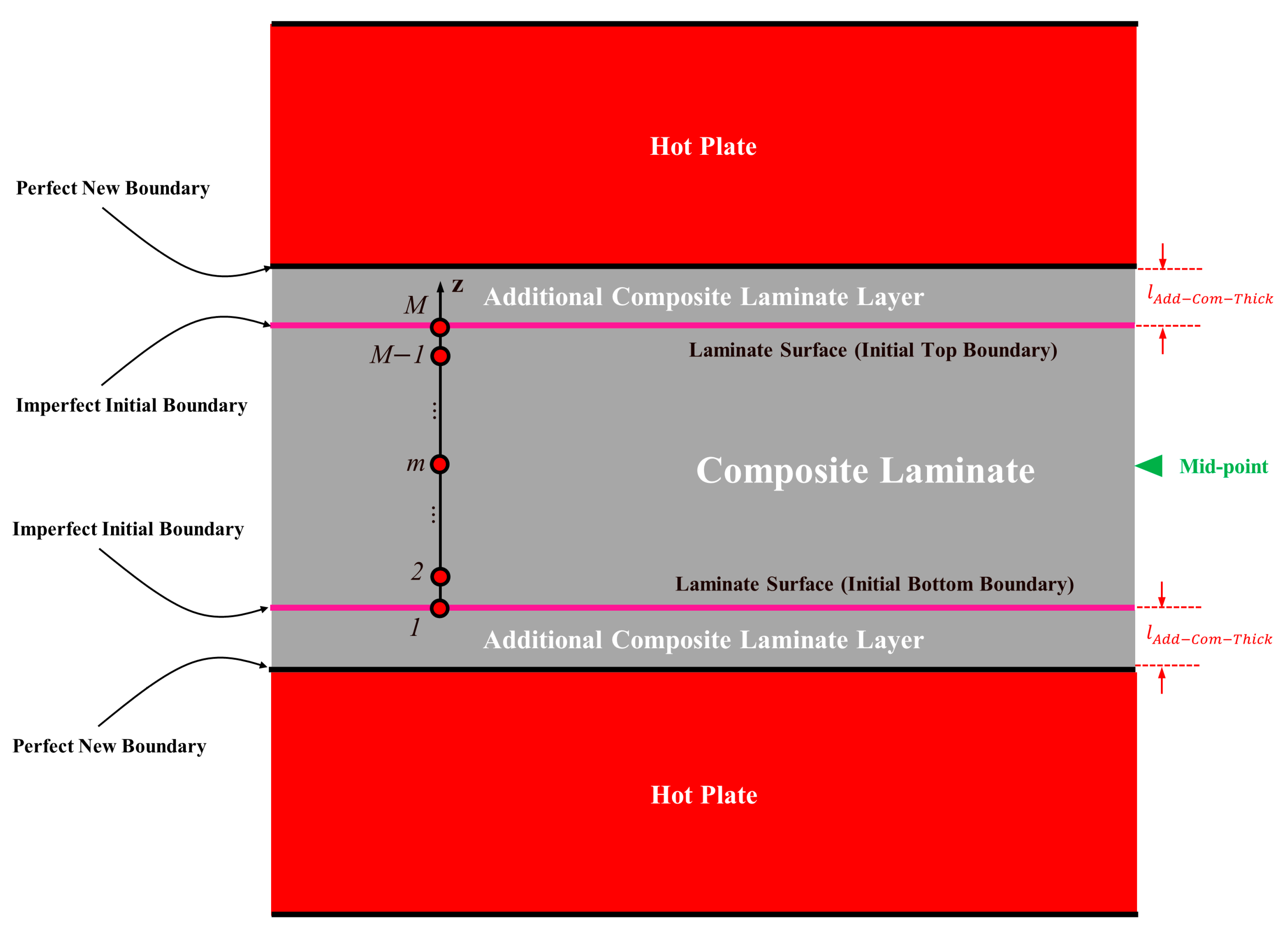
3.1. Thermal Simulation of Preheating Stage

The analysis presented in this section focuses on the thermal simulation of the preheating stage of the thermoforming process by employing the Finite Difference (FD) method with MATLAB implementation. The investigation aims to gain insights into the temperature distribution within the composite part during the preheating process. Three distinct preheating modes are studied, namely, the conductive, convective, and radiative modes. Figure 2 illustrates the schematic representation of the preheating process for each mode. While heat transfer within the composite part mainly occurs through conduction, the method by which heat is supplied to the composite part varies based on the selected preheating mode, necessitating a comprehensive analysis of each scenario.

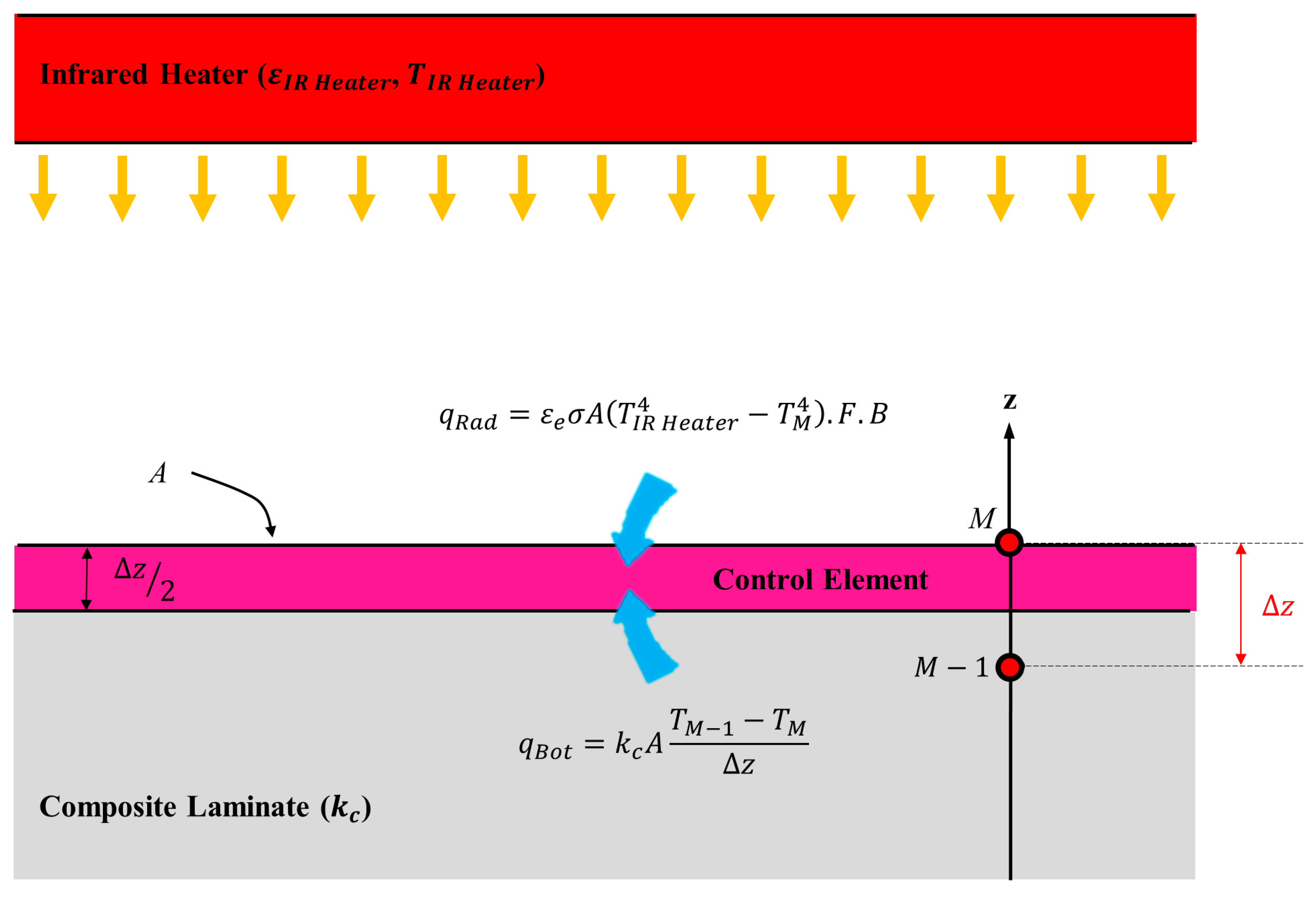
3.1.1. Analysis of Boundary Nodes

The preheating process can be conducted through different modes of heat transfer, each characterized by distinct formulations. This section explores the various preheating modes and provides a detailed explanation of their corresponding boundary conditions. Additionally, explicit finite difference (FD) formulations for these preheating modes are derived to aid in accurate and efficient numerical simulations. The explicit method is selected because it is easier to use, especially in computer coding [23,24]. To facilitate the analyses presented in the subsequent sections, an essential assumption is made, suggesting a uniform temperature distribution across the surfaces (boundaries) of the composite laminate. This assumption is considered reasonable, particularly when the thermal elements of the preheating stage have been activated for a sufficient duration, leading to the attainment of a steady-state temperature throughout the boundaries. Therefore, no temperature gradients are induced in-plane within the composite laminate. As a result, the analysis simplifies to the calculation of a 1-D temperature distribution solely through the laminate thickness. While this assumption may impact the accuracy of the results, the comparative nature of this study, which focuses on evaluating the relative performance of different preheating modes, would further justify its use.

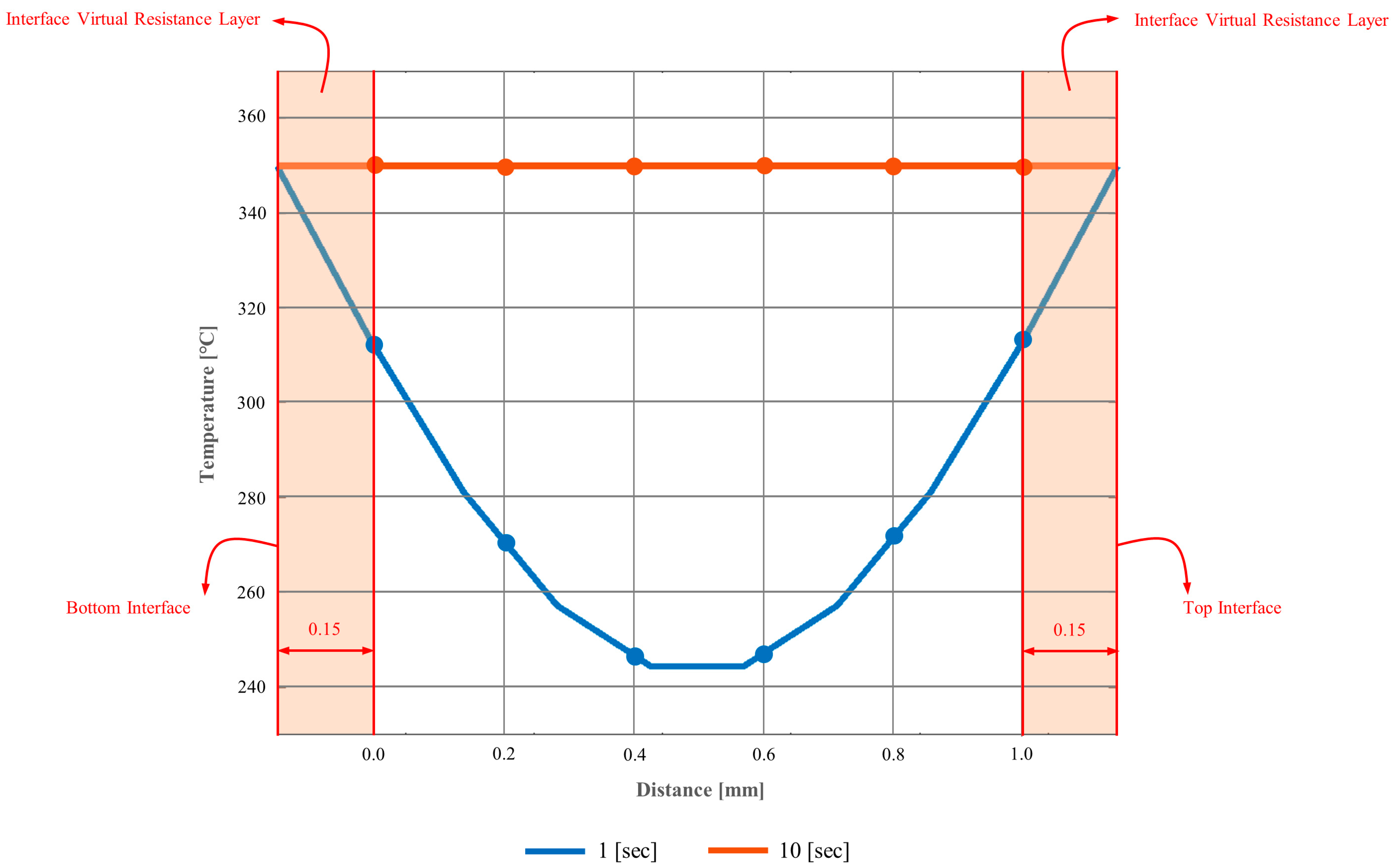
Boundary Nodes of the Conductive Mode of Preheating

To develop the formulation of the interface boundary condition for this mode of preheating, a control element, as illustrated in Figure 3, is introduced around the upper interface of the laminate and the hot plate. The relationship of the heat transfer rates entering the element and the rate of energy generated and stored within the element is achieved by following the framework outlined in Equation (1).

$$q_{Top}+q_{Bot}+\dot{q}={(\rho }_c{C_p}_c+{\rho }_{HP-Top}{C_p}_{HP-Top})∆V\frac{T_M^{i+1}-T_M^i}{∆t}$$

(1)

where $q_{Top}$, $q_{Bot}$, $\dot{q}$, ${\rho }_c$, ${C_p}_c$, ${\rho }_{HP-Top}$, ${C_p}_{HP-Top}$, $∆t$, $T$, $i$, and $∆V(=A∆z)$ arethe rate of heat transfer from the top hot plate to the control element, the rate of heat transfer from the composite laminate to the control element, the rate of heat generated in the control element, the density of the composite laminate, the specific heat capacity of the composite laminate, the density of the hot plate, the specific heat capacity of the hot plate, the time interval, the nodal temperature, the time step counter, and the volume of the control element (i.e., the surface area of the interface multiplied by the space interval), respectively.

Expanding Equation (1) further using an explicit finite difference formulation and considering the thermoplastic nature of the polymer matrix in the composite laminate (resulting in $\dot{q}=0$) leads to a relationship described in Equation (2):

$$k_{HP-Top}A\frac{T_{M+1}^i-T_M^i}{∆z}+k_{c}A\frac{T_{M-1}^i-T_M^i}{∆z}={(\rho }_c{C_p}_c+{\rho }_{HP-Top}{C_p}_{HP-Top})A ∆z \frac{T_M^{i+1}-T_M^i}{∆t}$$

(2)

here, $k_{HP-Top}$ and $k_c$ denote thermal conductivity of the hot plate and composite laminate, respectively. Let us assume ${\rho }_c{C_p}_c+{\rho }_{HP-Top}{C_p}_{HP-Top}=\beta$, $\acute{\alpha }=\frac{k_c}{\beta }$, and $\acute{\tau }=\frac{\acute{\alpha } ∆t}{{∆z}^2}$. By isolating $T_M^{i+1}$, we obtain an expression elucidating the temperature at the interface node:

$$T_M^{i+1}=\left(1-\acute{\tau }-\frac{k_{HP-Top} \acute{\tau }}{k_c}\right)T_M^i+\left(\acute{\tau }\right) T_{M-1}^i+\left(\frac{k_{HP-Top} \acute{\tau }}{k_c}\right)T_{M+1 or HP-Top}^i$$

(3)

Similarly, an analogous equation is derived for the lower interface:

$$T_1^{i+1}=\left(1-\acute{\tau }-\frac{k_{HP-Bot} \acute{\tau }}{k_c}\right)T_1^i+\left(\acute{\tau }\right) T_2^i+\left(\frac{k_{HP-Bot} \acute{\tau }}{k_c}\right)T_{HP-Bot}^i$$

(4)

The aforementioned equations were derived based on the assumption of having a perfect interface, which does not hold true in the conductive preheating stage. To take this imperfection into account, a thermal contact resistance is introduced, defined as follows:

$$R_{Contact}=\frac{1}{h_{Contact}}$$

(5)

where $R_{Contact}$ and $h_{Contact}$ are thermal contact resistance and thermal contact conductance, respectively. To incorporate this thermal contact resistance into our analysis, an approach involving an additional equivalent composite laminate thickness is adopted [25]. This involves the introduction of an additional composite laminate thickness ($l_{Add-Com-Thick}$) at each interface, the magnitude of which is determined by Equation (6):

$$l_{Add-Com-Thick}=R_{Contact}{k}_c$$

(6)

This consideration accounts for the imperfect nature of the interface between the hot plates and the composite laminate [26]. Figure 4 shows the added layer of composite which accounts for the contact resistance at the hot plate and composite laminate interface.

While the explicit method offers simplicity in comparison to the implicit method, its applicability is constrained by inherent time stability issues. Consequently, an upper threshold for the time step ($∆t$) must be established to ensure stability. To determine this upper limit, the stability criterion is put into practice, requiring that all coefficients of $T_m^i$ in the $T_m^{i+1}$ equation exceed or equal zero [25]. This criterion for the conductive mode of preheating leads to:

$$∆t\le \frac{{∆z}^2\beta }{k_c+\mathrm{m}\mathrm{a}\mathrm{x}(k_{HP-Top},k_{HP-Bot})}$$

(7)

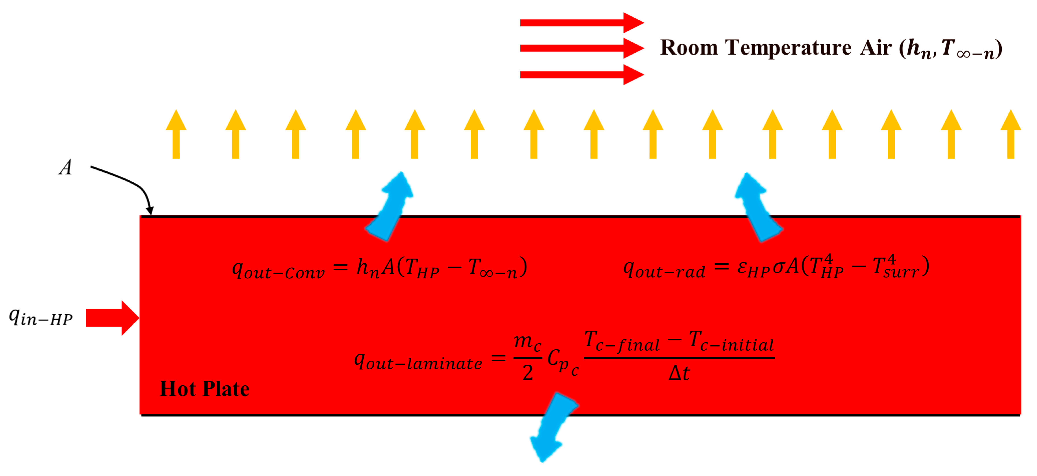
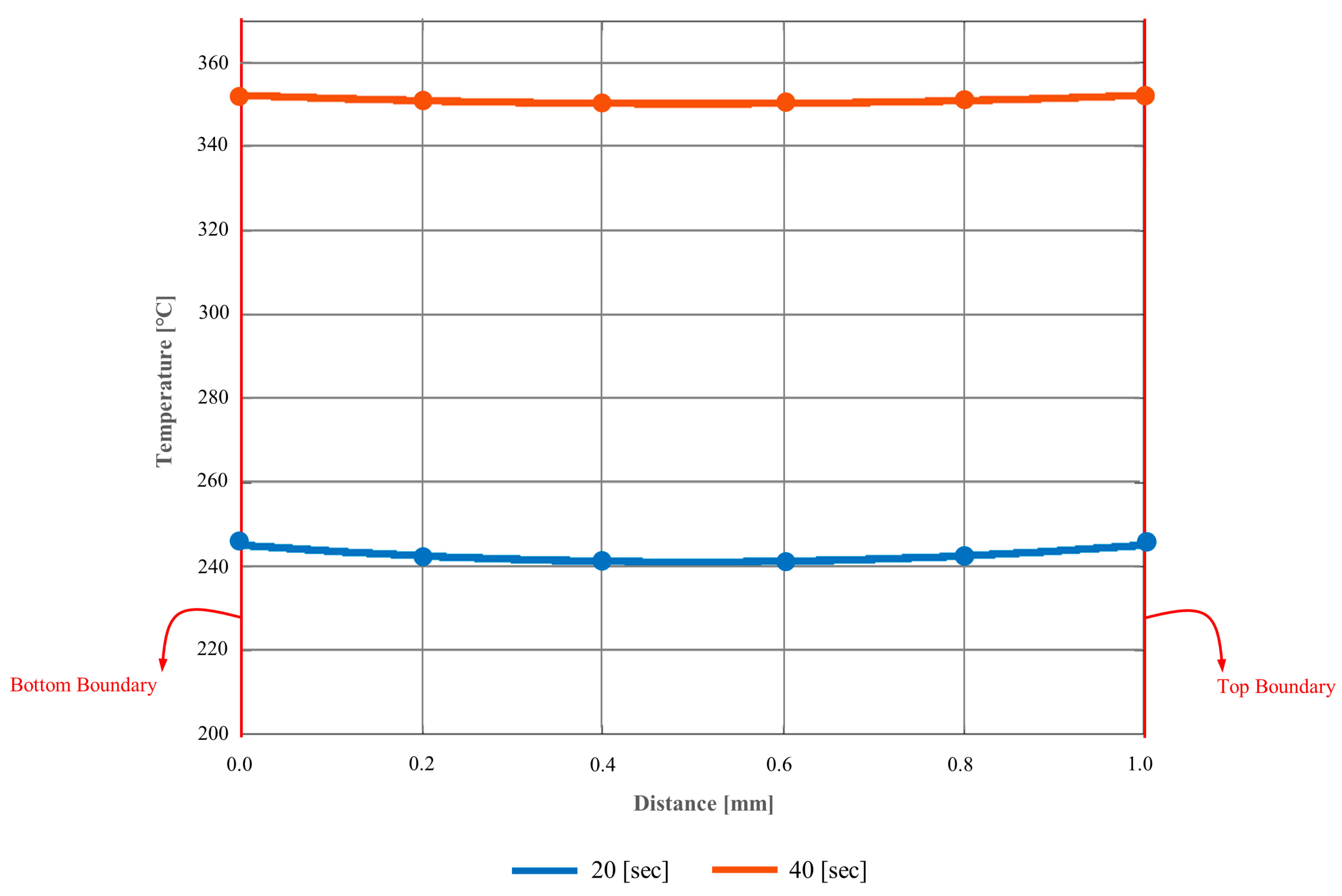
Boundary Nodes of the Convective Mode of Preheating

To model this boundary condition, a control element, as illustrated in Figure 5, is introduced at the upper boundary of the laminate. The formulation of the heat transfer rates entering the element and the rate of energy stored within the element is achieved by following the framework outlined in Equation (8).

$$q_{Bot}+q_{Conv}={\rho }_c{C_p}_c∆V\frac{T_M^{i+1}-T_M^i}{∆t}$$

(8)

In this context, $q_{Bot}$, $q_{Conv}$, and $∆V(=A\raisebox{1ex}{$∆z$}\!\left/ \!\raisebox{-1ex}{$2$}\right.)$ correspond to the rate of heat transfer from the composite laminate to the control element, the rate of heat transfer from the free stream to the control element, and the volume of the control element (i.e., the laminate’s surface area multiplied by half of the space interval), respectively.

Employing an explicit finite difference formulation to expand Equation (8) leads to the derivation of a resulting relationship, as shown in Equation (9):

$$k_{c}A\frac{T_{M-1}^i-T_M^i}{∆z}+hA\left(T_{\infty }-T_M\right)={\rho }_c{C_p}_c\frac{A∆z}{2}\frac{T_M^{i+1}-T_M^i}{∆t}$$

(9)

where $h$ and $T_{\infty }$ denote convective heat transfer coefficient and the temperature of the free stream, respectively. Let us assume $\alpha =\frac{k_c}{{\rho }_c{C_p}_c}$ and $\tau =\frac{\alpha ∆t}{{∆z}^2}$. Solving for $T_M^{i+1}$ yields the following expression for the temperature at the uppermost node:

$$T_M^{i+1}=\left(1-2\tau -2\tau \frac{h∆z}{k_c}\right)T_M^i+\left(2\tau \right)T_{M-1}^i+2\tau \frac{h∆z}{k_c}{T}_{\infty }$$

(10)

Similarly, an analogous equation is derived for the lowermost node:

$$T_1^{i+1}=\left(1-2\tau -2\tau \frac{h∆z}{k_c}\right)T_1^i+\left(2\tau \right)T_2^i+2\tau \frac{h∆z}{k_c}{T}_{\infty }$$

(11)

Note that in this scenario, we assume the laminate’s periphery is secured within a frame-style blank holder system, ensuring that both surfaces of the laminate remain exposed to hot air. To establish the upper threshold of the time step suitable for this particular setup, we again employ the stability criterion, the result of which is summarized in Equation (12).

$$∆t\le \frac{{∆z}^2{k}_c}{2\alpha \left(k_c+h∆z\right)}$$

(12)

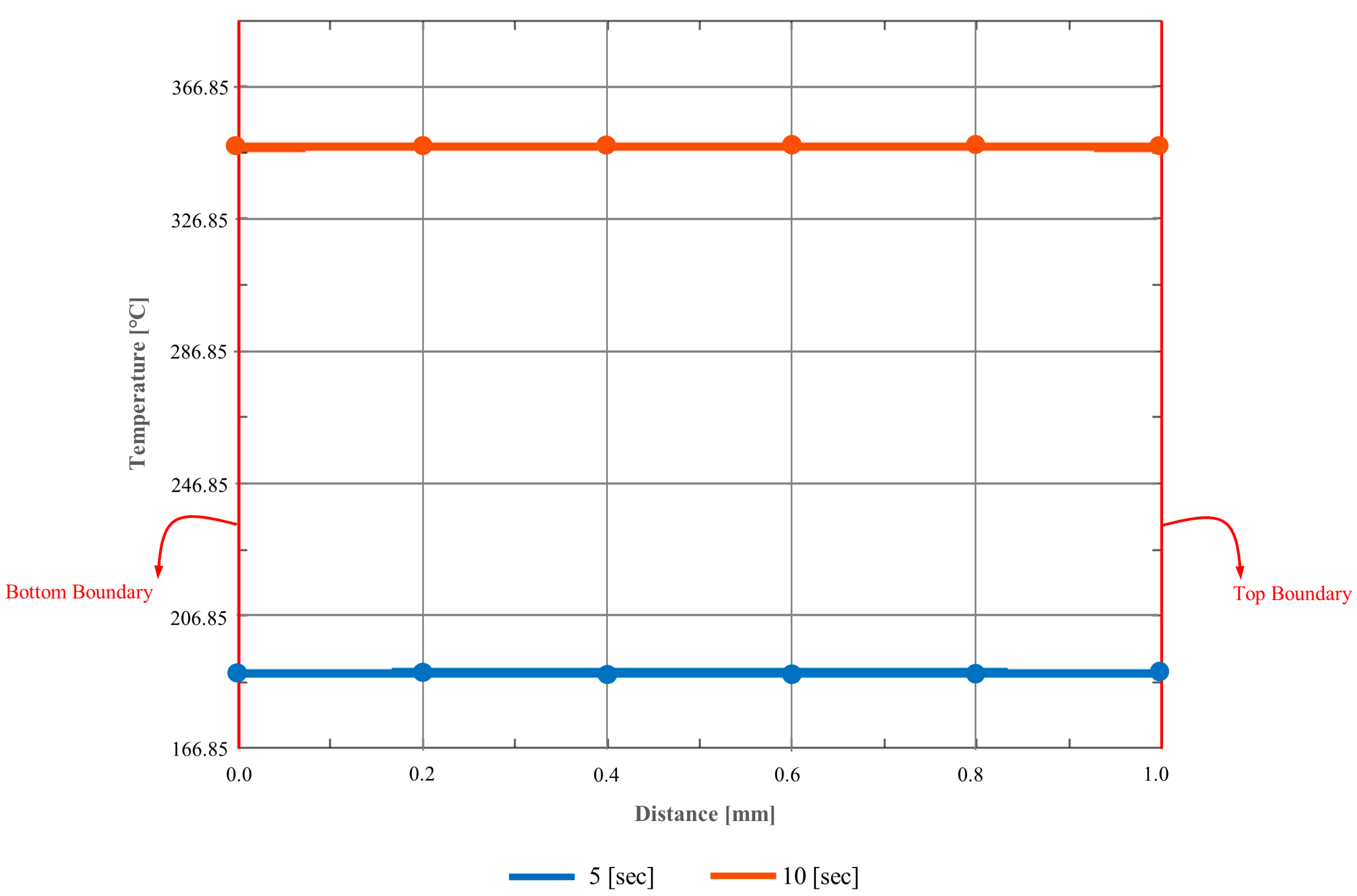
Boundary Nodes of the Radiative Mode of Preheating

To determine the temperature profile within the composite laminate during the radiative mode, a control element, depicted in Figure 6, is introduced at the upper boundary of the laminate, allowing us to formulate a heat transfer rate balance equation, as detailed in Equation (13).

$$q_{Bot}+q_{Rad-Abs-ex}={\rho }_c{C_p}_c∆V\frac{T_M^{i+1}-T_M^i}{∆t}$$

(13)

here, $q_{Bot}$, $q_{Rad-Abs-ex}$, and $∆V(=A\raisebox{1ex}{$∆z$}\!\left/ \!\raisebox{-1ex}{$2$}\right.)$ represent the rate of heat transfer from the composite laminate to the control element, the rate of absorbed heat transfer from the radiative source to the boundary control element, and the volume of the control element (i.e., the laminate’s surface area multiplied by half of the space interval), respectively.

Utilizing an explicit finite difference formulation to expand Equation (13) yields a resultant relationship, as described in Equation (14):

$$k_{c}A\frac{T_{M-1}^i-T_M^i}{∆z}+{\epsilon }_e\sigma A\left(T_{IR Heater}^4-{T_M^i}^4\right)·F·B_{ex}={\rho }_c{C_p}_c\frac{A∆z}{2}\frac{T_M^{i+1}-T_M^i}{∆t}$$

(14)

where ${\epsilon }_e$, $\sigma$, $F$, and $B_{ex}$ denote, in turn, effective emissivity, Stefan–Boltzmann constant, view factor, and the absorbed fraction of the radiation striking the boundary layer of the composite laminate. Effective emissivity in Equation (14) is calculated as follows:

$${\epsilon }_e=\frac{1}{\frac{1}{{\epsilon }_{IR Heater}}+\frac{1}{{\epsilon }_c}-1}$$

(15)

where ${\epsilon }_{IR Heater}$ and ${\epsilon }_c$ are the emissivity of the infrared heater and the composite laminate, respectively [27]. The absorbed fraction of the radiation striking the boundary layer of the composite laminate is calculated using the Beer–Lambert law [28]:

$$B_{ex}=1-e^{\left(\frac{-\acute{A}∆z}{2}\right)}$$

(16)

where $\acute{A}$ is the absorption coefficient of the material. By isolating $T_M^{i+1}$, we obtain an expression elucidating the temperature at the uppermost node:

$$T_M^{i+1}=\left(1-2\tau \right)T_M^i-\left(\frac{2{\epsilon }_e\sigma B_{ex}∆z \tau }{k_c}\right){T_M^i}^4+\left(2\tau \right)T_{M-1}^i+\left(\frac{2{\epsilon }_e\sigma B_{ex}∆z \tau }{k_c}\right)T_{IR Heater}^4$$

(17)

Similarly, an analogous equation is derived for the lowermost node:

$$T_1^{i+1}=\left(1-2\tau \right)T_1^i-\left(\frac{2{\epsilon }_e\sigma B_{ex}∆z \tau }{k_c}\right){T_1^i}^4+\left(2\tau \right)T_2^i+\left(\frac{2{\epsilon }_e\sigma B_{ex}∆z \tau }{k_c}\right)T_{IR Heater}^4$$

(18)

Applying the Beer–Lambert law to fiber-reinforced polymer composites is more complex than applying it to pure polymers. This complexity arises from the heterogenous nature of composites, which consist of fibers and polymer matrix. To use the Beer–Lambert law in composites, special considerations or assumptions shall be made. One such assumption is the homogeneity of the composite material, which allows for the definition of an effective absorption coefficient. This coefficient represents an average value that accounts for the combined effects of both the polymer and fiber. Due to intricate structure of composites, this effective absorption coefficient is typically determined empirically.

The determination of the upper limit for the time step ($∆t$) within this specific boundary condition mode relies on an iterative trial-and-error process to ensure the stability of the finite difference model. While in other modes of preheating, the interior nodes may not be directly affected by the boundary conditions, the dynamics of radiative heat transfer make it distinct. Radiative heat transfer stands apart from other mechanisms due to its unique ability to transmit through boundary layers and penetrate into lower levels, thus influencing the nodal temperatures of the interior nodes directly. Consequently, when computing the temperature profile of these interior nodes, it is important to account for the radiation energy transferred via the boundary layers. This concept will be elaborated upon in subsequent sections.

3.1.2. Analysis of Interior Nodes

While heat transfer from the environment to the composite laminate could occur through one or a combination of the mechanisms elucidated in Section 3.1, the primary mode of heat transfer within the laminate is through conduction. This statement holds true for both conductive and convective boundary conditions. However, in the case of radiation, an additional mechanism of heat transfer emerges within the composite laminate that needs to be considered in our analysis. Subsequent sections delve into a comprehensive explanation of heat transfer mechanisms pertaining to the interior nodes.

Interior Nodes of the Conductive and Convective Modes of Preheating

The primary mechanism of heat transfer within the composite laminate is conduction, which is governed by the partial differential equation, described in Equation (19).

$$k_c\left(\frac{{\partial }^{2}T}{\partial z^2}\right)={\rho }_c{C_p}_c\frac{\partial T}{\partial t}$$

(19)

Similarly to the boundary cases, we use an explicit finite difference formulation to solve this particular partial differential equation. Equation (20) outlines the explicit finite difference formulation applicable to the interior nodes of the composite laminate during the conductive and convective modes of preheating:

$$T_m^{i+1}=\tau \left(T_{m-1}^i+T_{m+1}^i\right)+\left(1-2\tau \right)T_m^i$$

(20)

Interior Nodes of the Radiative Modes of Preheating

When analyzing the temperature profile of the interior nodes within the composite laminate under the radiative preheating mode, an additional energy transfer term comes into play. This term accounts for the rate of radiation transmitted from the boundary layers to the interior layers. In the radiative preheating mode, as the heating element emits energy towards the composite surface, the majority of this energy is absorbed by the laminate (typically around 95% for a standard composite sheet [28]), with a smaller fraction being reflected. Among this non-reflected energy, a portion is absorbed by the laminate itself, while the remainder transmits through the material.

As previously detailed in Section 3.1.3, a fraction of the radiative energy gets absorbed by the boundary layer, characterized by its absorption rate $q_{Rad-Abs-ex}$. The rest of the energy is conveyed to the interior layers, where a fraction is absorbed by these layers. Additionally, a portion of the radiative energy, unabsorbed by either the boundary or interior layers, exits the laminate. By considering this energy transfer narrative, the heat transfer rate balance equation for the interior nodes can be expressed as follows (see Figure 7):

$$q_{Top}+q_{Bot}+q_{Rad-Abs-Top-in}+q_{Rad-Abs-Bot-in}={\rho }_c{C_p}_c∆V\frac{T_m^{i+1}-T_m^i}{∆t}$$

(21)

In the equation, $q_{Top}$, $q_{Bot}$, $q_{Rad-Abs-Top-in}$, $q_{Rad-Abs-Bot-in}$ denote the respective rates of conductive heat transfer from node $m+1$ to the control element and from node $m-1$ to the control element, and the respective radiative heat transfer rates from the top boundary layer to the control element and from the bottom boundary layer to the control element.

The expansion of Equation (21) using an explicit finite difference formulation leads to the derivation of a resultant relationship, as elaborated upon in Equation (22).

$$k_{c}A\frac{T_{m+1}^i-T_m^i}{∆z}+k_{c}A\frac{T_{m-1}^i-T_m^i}{∆z}+{q_{Rad-Abs-Top-in}}_m+{q_{Rad-Abs-Bot-in}}_m={\rho }_c{C_p}_c∆V\frac{T_m^{i+1}-T_m^i}{∆t}$$

(22)

${q_{Rad-Abs-Top-in}}_m$ and ${q_{Rad-Abs-Bot-in}}_m$ are calculated as follows:

$${q_{Rad-Abs-Top-in}}_m={\epsilon }_e\sigma A\left(T_{IR Heater}^4-{T_M^i}^4\right)·F·B_{m-Top}$$

(23)

$${q_{Rad-Abs-Bot-in}}_m={\epsilon }_e\sigma A\left(T_{IR Heater}^4-{T_1^i}^4\right)·F·B_{m-Bot}$$

(24)

Using the Beer–Lambert law [28], the nodal absorbed fraction of the radiation striking the composite laminate by the interior layers is calculated as follows:

$$B_{m-Top}=B_{in}{\left(1-B_{in}\right)}^{\left(M-m+1\right)-2}(1-B_{ex})$$

(25)

$$B_{m-Bot}=B_{in}{\left(1-B_{in}\right)}^{m-2}(1-B_{ex})$$

(26)

where $B_{in}=1-e^{(-\acute{A}∆z)}$. Let us assume that $B_{m-Total}=B_{m-Top}+B_{m-Bot}$. By isolating $T_m^{i+1}$ in Equation (22), we obtain an expression elucidating the temperature at the interior nodes of the composite laminate exposed to the radiative boundary condition:

$$T_m^{i+1}=\left(1-2\tau \right)T_m^i+\left(\tau \right)\left(T_{m+1}^i+T_{m-1}^i\right)+\left(\frac{\tau ∆z}{k_c}\right)\left(B_{m-Total}\right){\epsilon }_e\sigma F\left(T_{IR HEater}^4-{T_{M or 1}^i}^4\right)$$

(27)

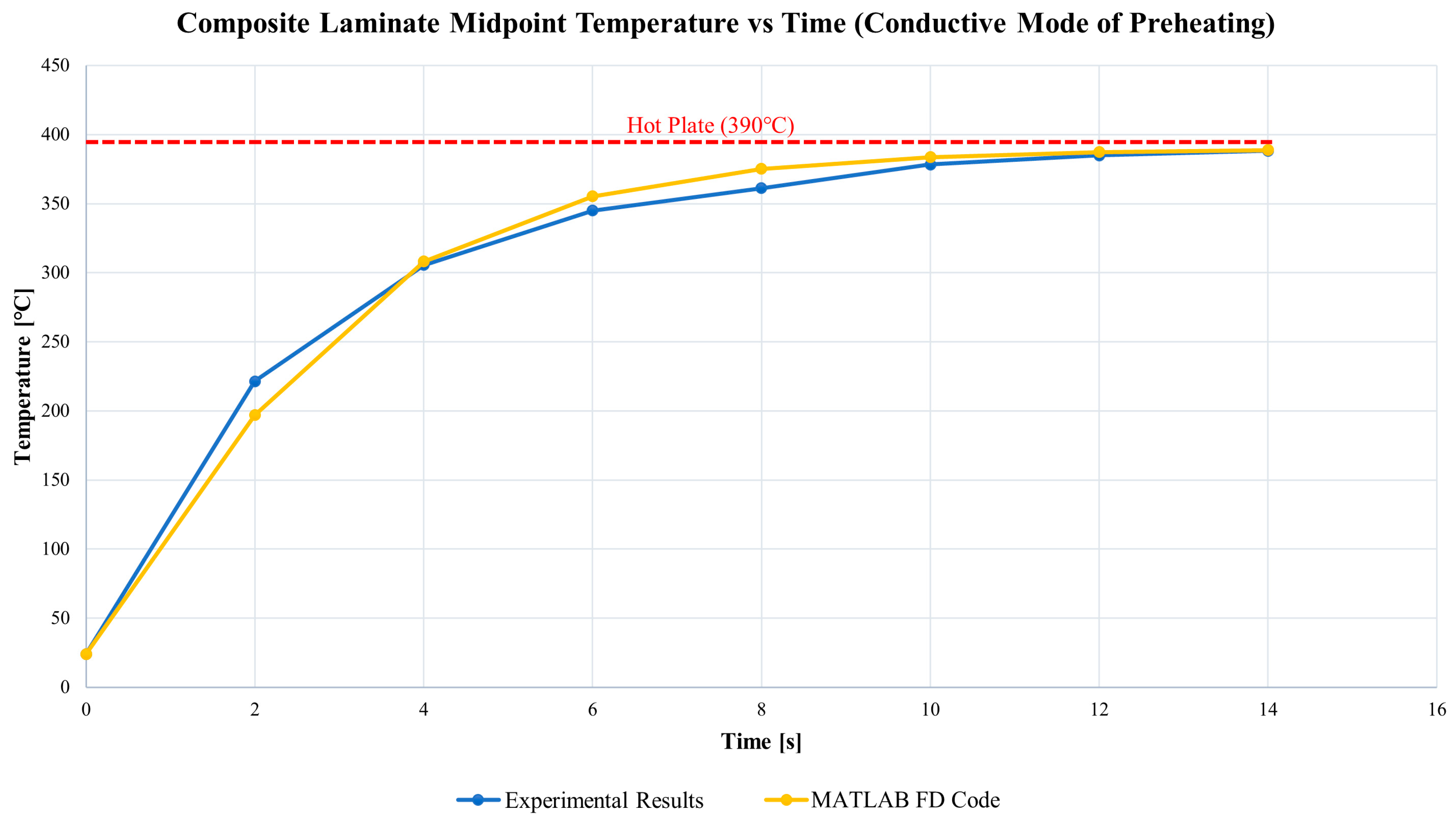
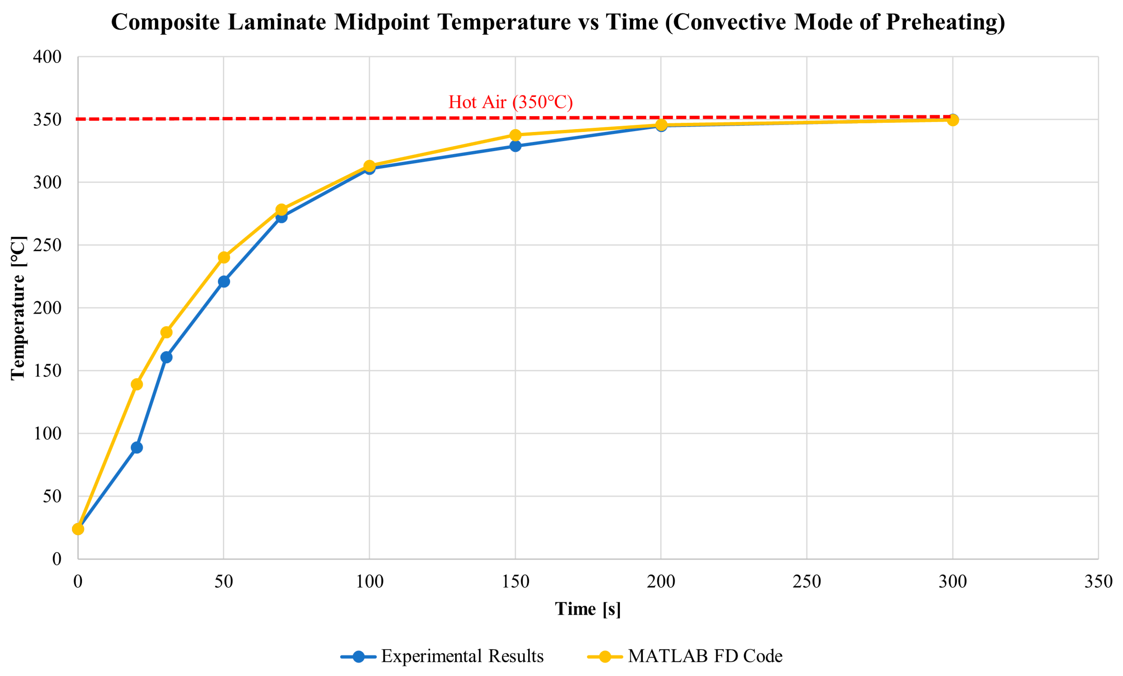
3.1.3. Finite Difference Model Validation

In the process of validating the finite difference formulations developed for the preheating modes, the support of experimental data from existing literature was leveraged [24,29]. MATLAB software (R2023a) was employed to simulate thermal phenomena during the preheating stage by using the finite difference formulations derived in this study. The validation process was first carried out for both the conductive and convective preheating modes through a comparison of results with those previously presented in [24]. The similarity in configurations between our study and the referenced results facilitated this validation.

Table 1. Key parameters and corresponding values utilized for the modeling of the conductive heat transfer mode.

Parameters	Simulation		Hot Plate (Mold)						Composite Laminate
	Number of Nodes	Initial Temperature of Laminate	Material	Conductive Heat Transfer Coefficient $({\mathit{k}}_{\mathit{H}\mathit{P}}$)	Temperature $({\mathit{T}}_{\mathit{H}\mathit{P}}$)	Density $({\mathit{\rho }}_{\mathit{H}\mathit{P}}$)	Specific Heat Capacity $({{\mathit{C}}_{\mathit{p}}}_{\mathit{H}\mathit{P}}$)	Steel-Composite Laminate Interface Conductance	Material	Thickness	Thermal Conductivity $({\mathit{k}}_{\mathit{c}}$)	Density$({\mathit{\rho }}_{\mathit{c}}$)	Specific Heat $({{\mathit{C}}_{\mathit{p}}}_{\mathit{c}}$)
Values	10	24	Steel	45	390	7850	490	650	APC-2/S4	0.0009	0.36	1615	1288
Units	N.A.	[$°\mathrm{C}$]	N.A.	$\left[\raisebox{1ex}{$\mathrm{W}$}\!\left/ \!\raisebox{-1ex}{$\mathrm{m}·°\mathrm{C}$}\right.\right]$	[$°\mathrm{C}$]	$\left[\raisebox{1ex}{$\mathrm{k}\mathrm{g}$}\!\left/ \!\raisebox{-1ex}{${\mathrm{m}}^3$}\right.\right]$	$\left[\raisebox{1ex}{$\mathrm{J}$}\!\left/ \!\raisebox{-1ex}{$\mathrm{k}\mathrm{g}·°\mathrm{C}$}\right.\right]$	$\left[\raisebox{1ex}{$\mathrm{W}$}\!\left/ \!\raisebox{-1ex}{${\mathrm{m}}^2·°\mathrm{C}$}\right.\right]$	N.A.	[$\mathrm{m}$]	$\left[\raisebox{1ex}{$\mathrm{W}$}\!\left/ \!\raisebox{-1ex}{$\mathrm{m}·°\mathrm{C}$}\right.\right]$	$\left[\raisebox{1ex}{$\mathrm{k}\mathrm{g}$}\!\left/ \!\raisebox{-1ex}{${\mathrm{m}}^3$}\right.\right]$	$\left[\raisebox{1ex}{$\mathrm{J}$}\!\left/ \!\raisebox{-1ex}{$\mathrm{k}\mathrm{g}·°\mathrm{C}$}\right.\right]$

summarizes the key parameters and their corresponding values (extracted from the reference data) used for modeling the conductive heat transfer mode of APC-2/S4 (PEEK-Carbon Fiber Reinforced Prepreg). Figure 8 presents a comparison between the simulation results and the experimental data as presented in [24]. The figure demonstrates a reasonable alignment between the experimental data and the numerical results derived from the finite difference model developed in MATLAB for the midpoint of the composite laminate.

An identical approach was undertaken to validate the MATLAB results pertaining to the convective preheating mode.

Table 2. Parameters and corresponding values adopted for modeling the convective heat transfer mode.

Parameters	Simulation		Free Stream (Hot Air)		Composite Laminate
	Number of Nodes	Initial Temperature of Laminate	Convective Heat Transfer Coefficient $(\mathit{h}$)	Temperature $({\mathit{T}}_{\mathit{\infty }}$)	Material	Thickness	Thermal Conductivity $({\mathit{k}}_{\mathit{c}}$)	Density $({\mathit{\rho }}_{\mathit{c}}$)	Specific Heat Capacity $({{\mathit{C}}_{\mathit{p}}}_{\mathit{c}}$)
Values	10	24	20	350	APC-2/S4	0.0009	0.36	1615	1288
Units	N.A.	[$°\mathrm{C}$]	$\left[\raisebox{1ex}{$\mathrm{W}$}\!\left/ \!\raisebox{-1ex}{${\mathrm{m}}^2·°\mathrm{C}$}\right.\right]$	[$°\mathrm{C}$]	N.A.	[$\mathrm{m}$]	$\left[\raisebox{1ex}{$\mathrm{W}$}\!\left/ \!\raisebox{-1ex}{$\mathrm{m}·°\mathrm{C}$}\right.\right]$	$\left[\raisebox{1ex}{$\mathrm{k}\mathrm{g}$}\!\left/ \!\raisebox{-1ex}{${\mathrm{m}}^3$}\right.\right]$	$\left[\raisebox{1ex}{$\mathrm{J}$}\!\left/ \!\raisebox{-1ex}{$\mathrm{k}\mathrm{g}·°\mathrm{C}$}\right.\right]$

provides an overview of the parameters and corresponding values adopted for modeling the convective heat transfer mode. Displayed in Figure 9 is a juxtaposition of simulation results and experimental data presented in [24] for the convective preheating mode. This figure highlights a favorable agreement between the experimental data and the numerical results derived through the MATLAB finite difference model for the midpoint of the composite laminate.

While [24] provided a reasonable basis for the experimental investigations of the conductive and convective preheating modes, the research presented in [29] is notable for its depth and comprehensiveness in studying the radiative preheating mode. Thus, the experimental investigation presented in [29] is selected to validate the MATLAB finite difference code.

Table 3. Parameters and corresponding values employed for the modeling of the radiative heat transfer mode.

Parameters	Simulation				Infrared Heater		Composite Laminate
	Number of Nodes	Initial Temperature of Laminate	Effective Emissivity $({\mathit{\epsilon }}_{\mathit{e}}$)	Stefan–Boltzmann Constant $(\mathit{\sigma }$)	View Factor $(\mathit{F}$)	Surface Temperature $({\mathit{T}}_{\mathit{I}\mathit{R} \mathit{H}\mathit{e}\mathit{a}\mathit{t}\mathit{e}\mathit{r}}$)	Material	Thickness	Thermal Conductivity $({\mathit{k}}_{\mathit{c}}$)	Density $({\mathit{\rho }}_{\mathit{c}}$)	Specific Heat Capacity $({{\mathit{C}}_{\mathit{p}}}_{\mathit{c}}$)	Absorption Coefficient ($\acute{\mathit{A}}$)
Values	10	297.15	0.81	5.67 $\times {10}^{-8}$	0.60	773.15	GF/PEI	0.0005	0.40	1910	890	980
Units	N.A.	[$\mathrm{K}$]	N.A.	$\left[\raisebox{1ex}{$\mathrm{W}$}\!\left/ \!\raisebox{-1ex}{${\mathrm{m}}^2$}\right.\right]$	N.A.	[$\mathrm{K}$]	N.A.	[$\mathrm{m}$]	$\left[\raisebox{1ex}{$\mathrm{W}$}\!\left/ \!\raisebox{-1ex}{$\mathrm{m}·\mathrm{K}$}\right.\right]$	$\left[\raisebox{1ex}{$\mathrm{k}\mathrm{g}$}\!\left/ \!\raisebox{-1ex}{${\mathrm{m}}^3$}\right.\right]$	$\left[\raisebox{1ex}{$\mathrm{J}$}\!\left/ \!\raisebox{-1ex}{$\mathrm{k}\mathrm{g}·\mathrm{K}$}\right.\right]$	$\left[\raisebox{1ex}{$1$}\!\left/ \!\raisebox{-1ex}{$\mathrm{m}$}\right.\right]$

outlines the parameters and their corresponding values (extracted from the reference data) employed for modeling the radiative heat transfer mode. As depicted in Figure 10, the numerical model’s temperature predictions for the surface point show a satisfactory alignment with the measured experimental data reported in [29], for the time interval after 25 s. A possible rationale for the discrepancy between numerical and experimental results during the first 25 s could be attributed to an assumption made in the MATLAB simulation—namely, the assumption of a steady radiation source right from the beginning of the process. In practice, this may not hold true, as the radiative heater might require a certain duration to attain a stable energy emission towards the composite laminate.

3.2. Consumed Energy of the Preheating Stage

3.2.1. Material

Analyzing the environmental impact of each preheating mode necessitates the calculations of the energy consumption. This study considers a flat 8-harness satin woven glass-fiber-reinforced polyetherimide (GF/PEI) composite produced by Toray with dimensions of 1 × 1 × 0.001 $\mathrm{m}$. The properties and the processing temperature of this material were reported in [29]. This specific composite laminate is chosen to serve as a representative for the blanks employed in composite thermoforming processes. The properties of the GF/PEI composite laminate used to calculate the energy consumption during the preheating phase are summarized in

Table 4. The properties of the GF/PEI composite laminate used to calculate the energy consumption during preheating.

Parameters	Constituents	Dimensions	Thermal Conductivity $({\mathit{k}}_{\mathit{c}}$)	Density $({\mathit{\rho }}_{\mathit{c}}$)	Specific Heat $({{\mathit{C}}_{\mathit{p}}}_{\mathit{c}}$)	Absorption Coefficient $\left(\acute{\mathit{A}}\right)$
Values	GF/PEI	1 × 1 × 0.001	0.40	1910	890	980
Units	N.A.	[$\mathrm{m}$]	$\left[\raisebox{1ex}{$\mathrm{W}$}\!\left/ \!\raisebox{-1ex}{$\mathrm{m}·°\mathrm{C}$}\right.\right]$	$\left[\raisebox{1ex}{$\mathrm{k}\mathrm{g}$}\!\left/ \!\raisebox{-1ex}{${\mathrm{m}}^3$}\right.\right]$	$\left[\raisebox{1ex}{$\mathrm{J}$}\!\left/ \!\raisebox{-1ex}{$\mathrm{k}\mathrm{g}·°\mathrm{C}$}\right.\right]$	$\left[\raisebox{1ex}{$1$}\!\left/ \!\raisebox{-1ex}{$\mathrm{m}$}\right.\right]$

.

3.2.2. Analysis of Energy Consumption of Modes of Preheating

The analysis of energy consumption for the preheating modes requires us to adjust their process parameters to ensure all modes of preheating are compared on the same grounds. To elucidate, the processing parameters for each preheating mode were adjusted to align their production rates. With a processing temperature of 350 $°\mathrm{C}$ for the GF/PEI composite laminate, MATLAB model parameters were tuned to achieve a midpoint temperature of 350 $°\mathrm{C}$ within 10 s. This 10 s interval solely accounts for the net heating time, excluding process setup.

Energy Consumption of the Conductive Mode of Preheating

The simulation parameters to obtain a midpoint temperature of 350 $°\mathrm{C}$ in 10 s were tailored in the MATLAB finite difference code as detailed in

Table 5. Simulation parameters to obtain a midpoint temperature of 350 °C in 10 s through the conductive mode of preheating.

Parameters	Simulation		Hot Plate (Mold)
	Number of Nodes	Initial Temperature of Laminate	Material	Conductive Heat Transfer Coefficient $({\mathit{k}}_{\mathit{H}\mathit{P}}$)	Temperature $({\mathit{T}}_{\mathit{H}\mathit{P}}$)	Density $({\mathit{\rho }}_{\mathit{H}\mathit{P}}$)	Specific Heat Capacity $({{\mathit{C}}_{\mathit{p}}}_{\mathit{H}\mathit{P}}$)	Aluminum-Composite Laminate Interface Conductance
Values	10	24	Aluminum	237	350	2700	897	2600
Units	N.A.	[$°\mathrm{C}$]	N.A.	$\left[\raisebox{1ex}{$\mathrm{W}$}\!\left/ \!\raisebox{-1ex}{$\mathrm{m}·°\mathrm{C}$}\right.\right]$	[$°\mathrm{C}$]	$\left[\raisebox{1ex}{$\mathrm{k}\mathrm{g}$}\!\left/ \!\raisebox{-1ex}{${\mathrm{m}}^3$}\right.\right]$	$\left[\raisebox{1ex}{$\mathrm{J}$}\!\left/ \!\raisebox{-1ex}{$\mathrm{k}\mathrm{g}·°\mathrm{C}$}\right.\right]$	$\left[\raisebox{1ex}{$\mathrm{W}$}\!\left/ \!\raisebox{-1ex}{${\mathrm{m}}^2·°\mathrm{C}$}\right.\right]$

. Figure 11 represents the temperature profile of the composite laminate corresponding to the conductive preheating mode with the tailored parameters.

These parameters are used to calculate the energy required to fulfill one functional unit. To determine this energy, the following relationship is used based on the heat transfer mechanisms shown in Figure 12:

$$q_{in-HP}=q_{out-Conv}+q_{out-Rad}+q_{out-Laminate}$$

(28)

where $q_{in-HP}$, $q_{out-Conv}$, $q_{out-Rad}$, and $q_{out-Laminate}$ are, in turn, the rate of heat transfer entering the hot plate, the rate of heat transfer existing the hot plate due to natural convection, the rate of heat transfer existing the hot plate due to radiation, and the rate of heat transfer exiting the hot plate to heat up the composite laminate.

This analysis assumes that the hot plates’ temperature remains constant during preheating. Equation (28) can be further expanded to:

$$q_{in-HP}=h_{n}A\left({T_{HP}-T}_{\infty -n}\right)+{\epsilon }_{HP}\sigma A(T_{HP}^4-T_{surr}^4)+\frac{m_c}{2}{C_p}_c\left(\frac{T_{c-Final}-T_{c-Initial}}{∆t}\right)$$

(29)

here, $h_n$, $T_{\infty -n}$, ${\epsilon }_{HP}$, $T_{c-Final}$, and $T_{c-Initial}$ denote the coefficient of natural convection heat transfer, the ambient temperature, the coefficient of emissivity of the aluminum hot plate, the final temperature of the laminate, and the initial temperature of the laminate, respectively. Note that in this analysis, the startup energy required to heat up the plates has been disregarded, as this energy, when divided by the considerable number of parts processed daily, becomes negligible.

For calculating the energy required per functional unit, $q_{in-HP}$ is multiplied by $∆t$ (10 s) and then by 2 to account for two hot plates in the conductive preheating mode. Using the summarized values in

Table 6. Parameters used in the conductive mode of preheating to calculate energy consumption per functional unit.

Parameters	Environment		Hot Plate (Mold)
	Temperature $({\mathit{T}}_{\mathit{\infty }-\mathit{n}} \mathbf{o}\mathbf{r} {\mathit{T}}_{\mathit{s}\mathit{u}\mathit{r}\mathit{r}}$)	Natural Convective Heat Transfer Coefficient $({\mathit{h}}_{\mathit{n}}$)	Material	Dimensions	Temperature $({\mathit{T}}_{\mathit{H}\mathit{P}}$)	Density $({\mathit{\rho }}_{\mathit{H}\mathit{P}}$)	Specific Heat Capacity $({{\mathit{C}}_{\mathit{p}}}_{\mathit{H}\mathit{P}}$)	Emissivity $({\mathit{\epsilon }}_{\mathit{H}\mathit{P}}$)
Values	24 or 297.15	5	Aluminum	1 × 1 × 0.010	350	2700	897	0.1
Units	[$°\mathrm{C}$] or [K]	$\left[\raisebox{1ex}{$\mathrm{W}$}\!\left/ \!\raisebox{-1ex}{${\mathrm{m}}^2·°\mathrm{C}$}\right.\right]$	N.A.	$\left[\mathrm{m}\right]$	[$°\mathrm{C}$]	$\left[\raisebox{1ex}{$\mathrm{k}\mathrm{g}$}\!\left/ \!\raisebox{-1ex}{${\mathrm{m}}^3$}\right.\right]$	$\left[\raisebox{1ex}{$\mathrm{J}$}\!\left/ \!\raisebox{-1ex}{$\mathrm{k}\mathrm{g}·°\mathrm{C}$}\right.\right]$	N.A.

, the energy consumption per functional unit is 0.17 kWh.

Energy Consumption of the Convective Mode of Preheating

The approach for determining the energy consumption of the convective preheating mode closely mirrors that of conductive preheating. Parameters derived from MATLAB are summarized in

Table 7. Simulation parameters to obtain a midpoint temperature of 350 °C in 10 s through the convective mode of preheating.

Parameters	Simulation		Free Stream (Hot Air)
	Number of Nodes	Initial Temperature of Laminate	Convective Heat Transfer Coefficient $(\mathit{h}$)	Temperature $({\mathit{T}}_{\mathit{\infty }}$)
Values	10	24	30	459
Units	N.A.	[$°\mathrm{C}$]	$\left[\raisebox{1ex}{$\mathrm{W}$}\!\left/ \!\raisebox{-1ex}{${\mathrm{m}}^2·°\mathrm{C}$}\right.\right]$	[$°\mathrm{C}$]

, achieving a 350 $°\mathrm{C}$ midpoint temperature within 40 s. For analysis, it is assumed that four parts are processed simultaneously in the oven, rendering an average processing time of 10 s for each laminate, consistent with other preheating modes. Figure 13 demonstrates the temperature profile of the composite laminate in convective preheating mode using the parameters summarized in Table 7.

To determine the energy required to fulfill one functional unit in a convection oven ($Q_{in-Oven}$), the following terms of energy are considered in the analysis:

$$Q_{in-Oven}=Q_{out-Laminate}+Q_{out-Loss}+Q_{out-Fan}$$

(30)

where $Q_{out-Laminate}$, $Q_{out-Loss}$, and $Q_{out-Fan}$ represent the energy needed to heat up the laminate, the heat (energy) loss occurring in the oven during the process, and the energy required by the fans to generate the necessary air velocity for the hot air ($T_{\infty }=459 ℃$) to obtain $h=30 \raisebox{1ex}{$\mathrm{W}$}\!\left/ \!\raisebox{-1ex}{${\mathrm{m}}^2·°\mathrm{C}$}\right.$, respectively. Generally, the average air velocity governs the heat transfer capability of the convective oven [30]. Heat transfer correlations have been formulated and can be employed to estimate the range of convective heat transfer coefficient as a function of the average air velocity and pressure [31,32]. For turbulent flow over a flat plate, the subsequent correlation has been proposed:

$$h=0.037{Re}^{4/5}{Pr}^{1/3}\frac{k_{Air}}{l_c}$$

(31)

here, $l_c$ is a characteristic flow length, $k_{Air}$ is the thermal conductivity of hot air, and $Re$ and $Pr$ are the Reynolds number and Prandtl number, respectively. The latter two dimensionless numbers are defined as follows:

$$Re=\frac{{\rho }_{Air}{v}_{Air}{l}_c}{{\mu }_{Air}}$$

(32)

$$Pr=\frac{{C_p}_{Air}{\mu }_{Air}}{k_{Air}}$$

(33)

where ${\rho }_{Air}$, $v_{Air}$, and ${\mu }_{Air}$ denote the density of hot air, the hot air velocity, and the viscosity of hot air, respectively. By employing Equations (31)–(33), the average velocity of the hot air ($v_{Air}$) required to obtain a specific convective heat transfer coefficient ($h$) is determined using the following equation:

$$v_{air}={\left(27.03 h {\left(\frac{{\mu }_{Air}}{{\rho }_{Air}{l}_c}\right)}^{4/5}{\left(\frac{k_{Air}}{{C_p}_{Air}{\mu }_{Air}}\right)}^{1/3}\left(\frac{l_c}{k_{Air}}\right)\right)}^{5/4}$$

(34)

On the other hand, the airflow velocity generated by an axial fan, $v_{Fan}$, can be calculated using the equation below [30]:

$$v_{Fan}=\sqrt[3]{\frac{2P_{Fan}}{{\rho }_{Air}{A}_{Fan}}}$$

(35)

where $P_{Fan}$ and $A_{Fan}$ are, in turn, the power of the fan’s motor and the cross-sectional flow area of the fan. Using the continuity equation, where $v_{Air}{A}_{Oven}=v_{Fan}{A}_{Fan}$, the following equation is derived:

$$P_{Fan}=\frac{1}{2}{v}_{Air}^3{\left(\frac{A_{Oven}}{A_{Fan}}\right)}^2{{\rho }_{Air} A}_{Oven}$$

(36)

here, $A_{Oven}$ is the cross-sectional area of the oven. Now, we can expand Equation (30) further to calculate the energy required to fulfill one functional unit in the convective mode of preheating:

$$Q_{in-Oven}=\frac{m_c}{2}{C_p}_c\left(\frac{T_{c-Final}-T_{c-Initial}}{∆t}\right)+Q_{out-Loss}+\frac{1}{4}.\left(\frac{1}{2}{v}_{Air}^3{\left(\frac{A_{Oven}}{A_{Fan}}\right)}^2{{\rho }_{Air} A}_{Oven} ∆t\right)$$

(37)

Similarly, in these calculations, the start-up energy required to raise the oven temperature to the processing level is neglected, as this energy, when divided by the large number of parts processed per day, becomes negligible. The energy needed to fulfill one functional unit is calculated using the values outlined in

Table 8. Parameters used in the convective mode of preheating to calculate energy consumption per functional unit.

Parameters	Convective Oven
	Heat Loss	Hot Air Viscosity $({\mathit{\mu }}_{\mathit{A}\mathit{i}\mathit{r}}$)	Hot Air Density $({\mathit{\rho }}_{\mathit{A}\mathit{i}\mathit{r}}$)	Oven-to-Fan Area Ratio $(\raisebox{1ex}{${\mathit{A}}_{\mathit{O}\mathit{v}\mathit{e}\mathit{n}}$}\!\left/ \!\raisebox{-1ex}{${\mathit{A}}_{\mathit{F}\mathit{a}\mathit{n}}$}\right.$)	Characteristic Flow Length $({\mathit{l}}_{\mathit{c}}$)	Hot Air Thermal Conductivity $({\mathit{k}}_{\mathit{A}\mathit{i}\mathit{r}}$)	Cross-Sectional Area of Oven $({\mathit{A}}_{\mathit{O}\mathit{v}\mathit{e}\mathit{n}}$)	Hot Air Specific Heat Capacity $({{\mathit{C}}_{\mathit{p}}}_{\mathit{A}\mathit{i}\mathit{r}}$)
Values	5	34.2 $\times {10}^{-6}$	0.4822	30	1	0.054	1	1082
Units	[%]	[kg/m·s]	$\left[\raisebox{1ex}{$\mathrm{k}\mathrm{g}$}\!\left/ \!\raisebox{-1ex}{${\mathrm{m}}^3$}\right.\right]$	N.A.	$\left[\mathrm{m}\right]$	$\left[\raisebox{1ex}{$\mathrm{W}$}\!\left/ \!\raisebox{-1ex}{$\mathrm{m}·°\mathrm{C}$}\right.\right]$	$\left[{\mathrm{m}}^2\right]$	$\left[\raisebox{1ex}{$\mathrm{J}$}\!\left/ \!\raisebox{-1ex}{$\mathrm{k}\mathrm{g}·°\mathrm{C}$}\right.\right]$

, resulting in a total of 1.79 kWh.

Energy Consumption of the Radiative Mode of Preheating

The simulated parameters for the radiative mode of preheating, required to attain a midpoint temperature of 350 $°\mathrm{C}$ within 10 s, are determined using MATLAB, as tabulated in

Table 9. Simulation parameters to obtain a midpoint temperature of 350 °C in 10 s through the radiative mode of preheating.

Parameters	Simulation				Infrared Heater
	Number of Nodes	Initial Temperature of Laminate	Effective Emissivity $({\mathit{\epsilon }}_{\mathit{e}}$)	Stefan–Boltzmann Constant $(\mathit{\sigma }$)	View Factor $(\mathit{F}$)	Surface Temperature $({\mathit{T}}_{\mathit{I}\mathit{R} \mathit{H}\mathit{e}\mathit{a}\mathit{t}\mathit{e}\mathit{r}}$)
Values	10	297.15	0.81	5.67 $\times {10}^{-8}$	0.60	1143.15
Units	N.A.	[$\mathrm{K}$]	N.A.	$\left[\raisebox{1ex}{$\mathrm{W}$}\!\left/ \!\raisebox{-1ex}{${\mathrm{m}}^2·{\mathrm{K}}^4$}\right.\right]$	N.A.	[$\mathrm{K}$]

. Figure 14 displays the temperature profile of the laminate as it undergoes heating through the radiative preheating mode, utilizing the parameters specified in Table 9.

To ascertain the energy consumption of the radiative energy source, the heat transfer balance for a unit of the radiation source fulfilling one functional unit is determined using the following equation:

$$q_{in-Rad}={\epsilon }_{IR Heater}\sigma A_{IR Heater}\left(T_{IR Heater}^4-T_{c-Initial}^4\right)+h_n{A}_{IR Heater}\left({T_{IR Hetaer}-T}_{\infty -n}\right)$$

(38)

where $A_{IR Heater}$ represents the surface area of the infrared heater and ${\epsilon }_{IR Heater}$ is the coefficient of emissivity of the infrared heater. The energy required to fulfill a single functional unit can be calculated by multiplying $q_{in-Rad}$ by the processing time ($∆t$), which is 10 s. Then, this product is multiplied by 2 due to the presence of two infrared heaters in the radiative preheating mode. Utilizing the values summarized in

Table 10. Parameters used in the radiative mode of preheating to calculate energy consumption per functional unit.

Parameters	Radiative Heater			Environment
	Infrared Heater Emissivity $({\mathit{\epsilon }}_{\mathit{I}\mathit{R} \mathit{H}\mathit{e}\mathit{a}\mathit{t}\mathit{e}\mathit{r}}$)	Surface Area of Infrared Heater $({\mathit{A}}_{\mathit{I}\mathit{R} \mathit{H}\mathit{e}\mathit{a}\mathit{t}\mathit{e}\mathit{r}}$)	Temperature of Infrared Heater $({\mathit{T}}_{\mathit{I}\mathit{R} \mathit{H}\mathit{E}\mathit{a}\mathit{t}\mathit{e}\mathit{r}}$)	Initial Temperature of Composite Laminate $({\mathit{T}}_{\mathit{c}-\mathit{I}\mathit{n}\mathit{i}\mathit{t}\mathit{i}\mathit{a}\mathit{l}}$)	Convective Heat Transfer Coefficient $({\mathit{h}}_{\mathit{n}}$)	Temperature $({\mathit{T}}_{\mathit{\infty }-\mathit{n}}$)
Values	0.85	1.00	1143.15	297.15	5	24
Units	N.A.	$\left[{\mathrm{m}}^2\right]$	$\left[\mathrm{K}\right]$	$\left[\mathrm{K}\right]$	$\left[\raisebox{1ex}{$\mathrm{W}$}\!\left/ \!\raisebox{-1ex}{${\mathrm{m}}^2·°\mathrm{C}$}\right.\right]$	[$°\mathrm{C}$]

, the energy needed to fulfill one functional unit amounts to 0.46 kWh.

4. Impact Assessment of Modes of Preheating

Life Cycle Impact Assessment (LCIA) is a critical step in evaluating the environmental impact of the preheating modes based on the theoretical energy consumption results obtained in Section 3.2. OpenLCA 2.0.2 software, integrated with the Product Environmental Footprints (PEF) database, is employed in this study to determine how the amount of energy required to fulfill one functional unit using different modes of preheating impacts the environment. Environmental footprints originated from the European Commission’s Single Market for Green Products initiative, which aims to develop a common methodology for the quantitative assessment of environmental impacts of products and processes to support their assessment and labeling [33].

The impact assessment method employed in this database relies on the PEF Mid-Point Indicator methodology [34]. As outlined in

Table 11. Impact categories of different modes of preheating at the midpoint level.

Preheating Modes		Conduction	Radiation	Convection
Reference Flow: Electrical Energy Required to Fulfill One Functional Unit $\left[\mathrm{k}\mathrm{W}-\mathrm{h}\right]$		0.17	0.46	1.79
Impact Categories	Climate Change $\left[\mathrm{k}\mathrm{g} {\mathrm{C}\mathrm{O}}_2 \mathrm{e}\mathrm{q}\right]$	1.525 $\times {10}^{-1}$	4.126 $\times {10}^{-1}$	1.606 $\times {10}^0$
	Ozon Depletion $\left[\mathrm{k}\mathrm{g} \mathrm{C}\mathrm{F}\mathrm{C}11 \mathrm{e}\mathrm{q}\right]$	5.603 $\times {10}^{-11}$	1.516 $\times {10}^{-10}$	5.900 $\times {10}^{-10}$
	Acidification $\left[\mathrm{m}\mathrm{o}\mathrm{l} \mathrm{H}+\mathrm{e}\mathrm{q}\right]$	3.959 $\times {10}^{-4}$	1.071 $\times {10}^{-3}$	4.169 $\times {10}^{-3}$
	Ecotoxicity—Freshwater $\left[\mathrm{C}\mathrm{T}\mathrm{U}\mathrm{e}\right]$	5.440 $\times {10}^{-3}$	1.472 $\times {10}^{-2}$	5.728 $\times {10}^{-2}$
	Eutrophication—Marine $\left[\mathrm{k}\mathrm{g} \mathrm{N} \mathrm{e}\mathrm{q}\right]$	8.427 $\times {10}^{-5}$	2.280 $\times {10}^{-4}$	8.873 $\times {10}^{-4}$
	Eutrophication—Freshwater $\left[\mathrm{k}\mathrm{g} \mathrm{P} \mathrm{e}\mathrm{q}\right]$	3.454 $\times {10}^{-7}$	9.346 $\times {10}^{-7}$	3.637 $\times {10}^{-6}$
	Eutrophication—Terrestrial $\left[\mathrm{m}\mathrm{o}\mathrm{l} \mathrm{N} \mathrm{e}\mathrm{q}\right]$	8.911 $\times {10}^{-4}$	2.411 $\times {10}^{-3}$	9.383 $\times {10}^{-3}$
	Human Toxicity—Cancer $\left[\mathrm{C}\mathrm{T}\mathrm{U}\mathrm{h}\right]$	1.196 $\times {10}^{-10}$	3.237 $\times {10}^{-10}$	1.259 $\times {10}^{-9}$
	Human Toxicity—Non-Cancer $\left[\mathrm{C}\mathrm{T}\mathrm{U}\mathrm{h}\right]$	2.663 $\times {10}^{-9}$	7.206 $\times {10}^{-9}$	2.804 $\times {10}^{-8}$
	Land Use $\left[\mathrm{P}\mathrm{t}\right]$	1.362 $\times {10}^0$	3.686 $\times {10}^0$	1.435 $\times {10}^{+1}$
	Water Use $\left[{\mathrm{m}}^3\right]$	1.955 $\times {10}^{-2}$	5.290 $\times {10}^{-2}$	2.059 $\times {10}^{-1}$
	Ionizing Radiation—Human Health $\left[\mathrm{k}\mathrm{B}\mathrm{q} \mathrm{U}235 \mathrm{e}\mathrm{q}\right]$	6.324 $\times {10}^{-2}$	1.711 $\times {10}^{-1}$	6.659 $\times {10}^{-1}$
	Particulate Matter $\left[\mathrm{d}\mathrm{i}\mathrm{s}\mathrm{e}\mathrm{a}\mathrm{s}\mathrm{e} \mathrm{i}\mathrm{n}\mathrm{c}.\right]$	3.733 $\times {10}^{-9}$	1.010 $\times {10}^{-8}$	3.930 $\times {10}^{-8}$
	Photochemical Ozone Formation—Human Health $\left[\mathrm{k}\mathrm{g} \mathrm{N}\mathrm{M}\mathrm{V}\mathrm{O}\mathrm{C} \mathrm{e}\mathrm{q}\right]$	2.349 $\times {10}^{-4}$	6.356 $\times {10}^{-4}$	2.473 $\times {10}^{-3}$
	Resource Use—Fossils $\left[\mathrm{M}\mathrm{J}\right]$	2.595 $\times {10}^0$	7.022 $\times {10}^0$	2.732 $\times {10}^{+1}$
	Resource Use—Minerals and Metals $\left[\mathrm{k}\mathrm{g} \mathrm{S}\mathrm{b} \mathrm{e}\mathrm{q}\right]$	5.064 $\times {10}^{-8}$	1.370 $\times {10}^{-7}$	5.332 $\times {10}^{-7}$

, PEF includes sixteen impact categories at the midpoint level, which are determined for the different modes of preheating based on their corresponding energy consumptions. Note that for this study, the impact assessment of each preheating mode is conducted by considering two basic processes to generate the reference flow: the medium voltage grid-mix electricity generation and delivery process (1–60 kV), as well as the conservation from medium voltage to low voltage process (240–600 V) that is commonly used by the majority of the industry sectors employing the thermoforming process.

5. Results and Discussion

The global market size of thermoplastic composites was estimated at USD 32.21 billion in 2021 and is expected to increase to USD 62.62 billion in 2030 [35]. The demand for thermoplastic composites is on the rise on account of their high impact resistance, unique processing possibilities, lightweight properties, strength, and environmental advantages [36]. When converting the estimated dollar value to the estimated volume of thermoplastic composites used in the market, it is projected that over 1 million cubic meters of thermoplastic composites will be used annually. This volume can be hypothetically equated to 1 billion units of the relatively thin 1 × 1 × 0.001 m laminates investigated in this study.

Since thermal processing is the dominant method used for thermoplastic composites before shaping, a straightforward upper–lower bound calculation suggests that a potential reduction of 1.45 billion kg of CO₂ per year is achievable if conductive preheating is chosen over the convective mode of preheating for relatively thin laminates in the global thermoplastic composite industry. This type of theoretical analysis underscores the importance of the decisions made by manufacturing leaders in incorporating environmental impacts into the design of products and their manufacturing processes.

While the radiative mode of preheating is the most-commonly employed technique for heating thermoplastic composites [37], a comparison of energy consumption between the radiative and conductive modes reveals room for improvement, with a well-considered choice between these two preheating methods. According to Hertwich [38], “Sustainable solutions, even if they do not achieve universal market penetration, are important because they indicate a development alternative, influence the development of conventional products, and may be adopted in situations of crisis”. Therefore, it is evident that even small improvements in the manufacturing processes of thermoplastic composites can be significant steps toward creating a more sustainable world. This is further emphasized when considering Figure 15, which schematically illustrates the relationship between effects and emissions.

As depicted in the graph, the impact on the environment varies depending on the amount of emissions. When emissions are minimal, the effect on the environment may be negligible. However, as the accumulated emissions increase over several decades or centuries, the adverse impact becomes substantially larger [39]. Hence, regardless of our current level of emissions, we should strive to minimize the emissions from our processes to delay the significant adverse environmental consequences of our actions. This study demonstrates the potential for notable reductions in environmental impacts through the thermal processing of thermoplastic composites.

In light of the preceding discussion, it is of utmost importance to develop practical techniques that harness the benefit of conductive preheating in thermoplastic composite processing, particularly for relatively thin to medium-thickness laminates. Although there are limitations associated with thermal processing using the conductive preheating method [40], such as the risk of composite material sticking to hot plates, the substantial difference in environmental impact between these methods justifies further research to address these challenges. Companies engaged in thermal processing of thermoplastic composites are strongly encouraged to proactively explore and address the technical challenges associated with adopting the conductive preheating mode, particularly when processing relatively thin to medium-thickness composite laminates.

On another note, when comparing the environmental impact of material production for thermoplastic composites, specifically PEI and fiberglass in this case, with the various preheating methods, it becomes evident that the preheating process can consume energy equivalent to as much as 13 percent of the material production (i.e., 14.17 kg of CO₂ emissions for material production [33] compared to 1.79 kg of CO₂ emissions when using convective preheating for the relatively thin laminate cases). This comparison also highlights the significant role of the preheating process throughout the entire life cycle of thermoplastic composite parts, which must be taken into serious consideration.

Viewing this study from another perspective helps us recognize how process parameters can be adjusted to reduce the environmental impacts of each process. Historically, most optimization efforts have been primarily focused on enhancing process productivity, reducing production cost, and improving final product quality [41]. The environmental impact perspective received comparatively less attention or was often overlooked.

An analysis of the conductive preheating process reveals the interrelation between energy consumption and, consequently, the environmental impact with various process parameters. Figure 16a presents a spider diagram that illustrates the influence of process parameters on energy consumption of the conductive preheating mode. The graph shows the sensitivity of energy consumption, and consequently, environmental impact, to changes in process parameters.

In this study, One-Factor-At-A-Time (OFAT) sensitivity analysis is employed, in which a Sensitivity Index (SI) is defined as follows:

$$SI=\frac{\raisebox{1ex}{$∆\mathsf{\Gamma }$}\!\left/ \!\raisebox{-1ex}{$\mathsf{\Gamma }$}\right.}{\raisebox{1ex}{$∆\varrho $}\!\left/ \!\raisebox{-1ex}{$\varrho $}\right.}$$

(39)

where $\mathsf{\Gamma }$, $∆\mathsf{\Gamma }$, $\varrho$, and $∆\varrho$ are the output parameter at the base value of the input, the change in the output parameter, the base value of the input parameter, and the change in the input parameter from the base value, respectively. This approach is a straightforward method for assessing the impact of individual input parameters on process output.

As demonstrated in Figure 16a, the most influential process parameters in the conductive mode of preheating are the temperature of the hot plate and the interface surface property. This highlights the importance of optimizing these process parameters to minimize energy consumption and environmental impacts in this preheating mode.

The same analysis was conducted for the convective mode of preheating, as illustrated in Figure 16b. The sensitivity analysis reveals that the velocity of the hot fluid and its viscosity have the most significant influence on energy consumption. While other parameters do affect energy consumption, these two parameters have a notably greater impact. It is worth noting that these process parameters are interrelated with the temperature of the oven; therefore, an integrated process parameter optimization approach should be considered for realistic and practical results.

In the sensitivity analysis of the radiative mode of preheating as shown in Figure 16c, it is evident that the view factor has the most pronounced impact on energy consumption in this mode. Hence, to reduce energy consumption in this process, the radiation set-up should be designed to maximize the view factor, bringing it close to unity. This theoretical study lays the foundation for a parametric optimization process with the primary goal of minimizing energy consumption at this stage of the manufacturing process and its associated environmental impacts.

While this theoretical investigation highlights the importance of selecting the conductive mode of preheating for relatively thin composite laminates, it is crucial to note that the choice of the most efficient preheating method also depends on the thickness of the laminate. As shown in Figure 17a, the trend of energy consumption for different preheating modes would vary with changes in laminate thickness. The analysis of this trend reveals that the conductive mode is the most efficient method for preheating composite laminates within a relatively thin to medium-thickness range (i.e., 1–10 mm thick laminates). However, as the laminate thickness increases, the convective and radiative modes of preheating become more competitive and even more efficient, as depicted in Figure 17b, where the normalized energy consumption for laminates with different thicknesses referenced to the conductive mode is shown. Therefore, it is imperative to determine the most efficient mode of preheating for thermoplastic composite laminates based on their material and geometrical properties to ensure minimal environmental impacts associated with the manufacturing process selection.

6. Conclusions

In the current study, the preheating stage of the thermoforming process for thermoplastic composites was theoretically modeled to investigate its environmental impact. The analysis revealed that the preheating process significantly contributes to the life cycle assessment of thermoplastic composite parts. To elucidate, the environmental impact of the preheating process using the convection method for relatively thin laminates amounts to as much as 13 percent of the composite material production. Furthermore, the study demonstrated that conductive preheating has the lowest energy consumption (i.e., 0.17 $\mathrm{k}\mathrm{W}\mathrm{h}$) and environmental impact for relatively thin laminates, while the convective preheating mode exhibits the highest (i.e., 1.79 $\mathrm{k}\mathrm{W}\mathrm{h}$). This substantial difference underscores the importance of considering the environmental impact of these manufacturing methods when designing manufacturing processes for the thermoplastic composites. The radiative mode of preheating, which is the most common technique in thermal processing of thermoplastic composites, falls in the middle position in terms of energy consumption and environmental impact for relatively thin laminates. However, the difference with the conductive preheating method remains significant (i.e., 2.7 times larger). Additionally, a sensitivity analysis was conducted, revealing how sensitive energy consumption and environmental impact are to the manufacturing process parameters. For conductive preheating, the temperature of the hot plates and their interface properties with the composite laminate were found to have the highest impact. In the case of convection preheating, fluid velocity and viscosity had the most significant impact. In radiative preheating, the view factor emerged as one of the most influential factors. It was also discussed that laminate thickness impacts the energy consumption trend in different modes of preheating, making the convective and radiative modes of preheating more competitive or even more efficient as laminate thickness increases.

References

1. Arockiam, N.J.; Jawaid, M.; Saba, N. Sustainable bio composites for aircraft components. In Sustainable Composites for Aerospace Applications; Woodhead Publishing: Sawston, UK, 2018; pp. 109–123. [Google Scholar]
2. Sun, X.; Wang, P.; Ferris, T.; Lin, H.; Dreyfus, G.; Gu, B.; Zaelke, D.; Wang, Y. Fast action on short-lived climate pollutants and nature-based solutions to help countries meet carbon neutrality goals. Adv. Clim. Chang. Res. 2022, 13, 564–577. [Google Scholar] [CrossRef]
3. Liu, N.; Wang, Y.; Bai, Q.; Liu, Y.; Wang, P.S.; Xue, S.; Yu, Q.; Li, Q. Road life-cycle carbon dioxide emissions and emission reduction technologies: A review. J. Traffic Transp. Eng. 2022, 9, 532–555. [Google Scholar] [CrossRef]
4. Narayanan, R.G.; Gunasekera, J.S. Sustainable Manufacturing Processes; Elsevier: Amsterdam, The Netherlands, 2023. [Google Scholar]
5. Singh, M.; Ohji, T.; Asthana, R. Progress and Prospect. In Green and Sustainable Manufacturing of Advanced Materials; Elsevier: Amsterdam, The Netherlands, 2016; pp. 3–10. [Google Scholar]
6. Choi, A.C.K.; Kaebernick, H.; Lai, W.H. Manufacturing processes modelling for environmental impact assessment. J. Mater. Process. Technol. 1997, 70, 231–238. [Google Scholar] [CrossRef]
7. Song, Y.S.; Youn, J.R.; Gutowski, T.G. Life cycle energy analysis of fiber-reinforced composites. Compos. Part A 2009, 40, 1257–1265. [Google Scholar] [CrossRef]
8. Francioso, V.; Lopez-Arias, M.; Moro, C.; Jung, N.; Velay-Lizancos, M. Impact of curing temperature on the life cycle assessment of sugarcane bagasse ash as a partial replacement of cement in mortars. Sustainability 2023, 15, 142. [Google Scholar] [CrossRef]
9. Parameswaranpillai, J.; Vijayan, D. Life Cycle Assessment (LCA) of Epoxy-Based Materials. In Micro- and Nanostructured Epoxy/Rubber Blends; Wiley: Hoboken, NJ, USA, 2014; pp. 421–432. [Google Scholar]
10. Chatzipanagiotou, K.R.; Antypa, D.; Petrakli, F.; Karatza, A.; Pik, K.; Bogacka, M.; Poranek, N.; Werle, S.; Amanatides, E.; Mataras, D.; et al. Life Cycle Assessment of Composites Additive Manufacturing Using Recycled Materials. Sustainability 2023, 15, 12843. [Google Scholar] [CrossRef]
11. Zhao, M.; Dong, Y.; Guo, H. Comparative life cycle assessment of composite structures incorporating uncertainty and global sensitivity analysis. Eng. Struct. 2021, 242, 112394. [Google Scholar] [CrossRef]
12. Bachmann, J.; Hidalgo, C.; Bricout, S. Environmental analysis of innovative sustainable composites with potential use in aviation sector—A life cycle assessment review. Sci. China-Technol. Sci. 2017, 60, 1301–1317. [Google Scholar] [CrossRef]
13. Richard, D.; Hong, T.; Hastak, M.; Mirmiran, A.; Salem, O. Life-cycle performance model for composites in construction. Compos. Part B 2007, 38, 236–246. [Google Scholar] [CrossRef]
14. Ramachandran, K.; Constance, L.; Gnanasagaran, A.V. Life cycle assessment of carbon fiber and bio-fiber composites prepared via vacuum bagging technique. J. Manuf. Process. 2023, 89, 124–131. [Google Scholar] [CrossRef]
15. Al-Lami, A.; Hilmer, P.; Sinapius, M. Eco-efficiency assessment of manufacturing carbon fiber reinforced polymers (CFRP) in aerospace industry. Aerosp. Sci. Technol. 2018, 79, 669–678. [Google Scholar] [CrossRef]
16. Khalil, Y.F. Eco-efficient lightweight carbon-fiber reinforced polymer for environmentally greener commercial aviation industry. Sustain. Prod. Consum. 2017, 12, 16–26. [Google Scholar] [CrossRef]
17. Hosseini, A.; Kashani, M.H.; Sassani, F.; Milani, A.; Ko, F.K. A mesoscopic analytical model to predict the onset of wrinkling in plain woven preforms under bias extension shear deformation. Materials 2017, 10, 1184. [Google Scholar] [CrossRef] [PubMed]
18. Kumar, K.; Zindani, D.; Davim, J.P. Sustainable Manufacturing and Design; Woodhead Publishing: Sawston, UK, 2021. [Google Scholar]
19. Längauer, M.; Zitzenbacher, G.; Stadler, H.; Hochenauer, C. Enhanced simulation of infrared heating of thermoplastic composites prior to forming under consideration of anisotropic thermal conductivity and deconsolidation by means of novel physical material models. Polymers 2022, 14, 3331. [Google Scholar] [CrossRef] [PubMed]
20. Kirby, M.; Naderi, A.; Palardy, G. Predictive thermal modeling and characterization of ultrasonic consolidation process for thermoplastic composites. J. Manuf. Sci. Eng. 2023, 145, 031009. [Google Scholar] [CrossRef]
21. Koerdt, M.; Koerdt, M.; Grobrug, T.; Skowronek, M.; Herrmann, A. Modelling and analysis of the thermal characteristic of thermoplastic composites from hybrid textiles during compression moulding. J. Thermoplast. Compos. Mater. 2022, 35, 127–146. [Google Scholar] [CrossRef]
22. Längauer, M.; Brunnthaller, F.; Zitzenbacher, G.; Burgstaller, C.; Hochenauer, C. Modeling of the anisotropic thermal conductivity of fabrics embedded in a thermoplastic matrix system. Polym. Compos. 2021, 42, 2050–2060. [Google Scholar] [CrossRef]
23. Moghadamazad, M.; Hoa, S.V. Models for heat transfer in thermoplastic composites made by automated fiber placement using hot gas torch. Compos. Part C Open Access 2022, 7, 100214. [Google Scholar] [CrossRef]
24. Cunningham, J.E.; Monaghan, P.F.; Brogan, M.T.; Cassidy, S.F. Modelling of pre-heating of flat panels prior to press forming. Compos. Part A 1997, 28, 17–24. [Google Scholar] [CrossRef]
25. Cengel, Y.A.; Ghajar, A.J. Heat and Mass Transfer: Fundamentals & Applications; McGraw-Hill Education: New York, NY, USA, 2015. [Google Scholar]
26. Gibbins, J. Thermal Contact Resistance of Polymer Interfaces. Master’s Thesis, University of Waterloo, Waterloo, ON, Canada, 2006. [Google Scholar]
27. Watlow Electric Manufacturing Company. Radiant Heating with Infrared: A Technical Guide to Understanding and Applying Infrared Heaters; Watlow Electric Manufacturing Company: Saint Louis, MO, USA, 1997. [Google Scholar]
28. Ajersch, M. Modeling and Real-Time Control of Sheet Reheat Phase in Thermoforming. Master’s Thesis, McGill University, Montreal, QC, USA, 2004. [Google Scholar]
29. Nardi, D.; Sinke, J. Design analysis for thermoforming of thermoplastic composites: Prediction and machine learning-based optimization. Compos. Part C Open Access 2021, 5, 100126. [Google Scholar] [CrossRef]
30. Fernlund, G.; Mobuchon, C.; Zobeiry, N. Autoclave Processing. In Comprehensive Composite Materials II; Elsevier Ltd.: Amsterdam, The Netherlands, 2018; pp. 42–62. [Google Scholar]
31. Young, W.C.; Budynas, R.G.; Sadegh, A.M. Roark’s Formulas for Stress and Strain; McGraw-Hill: New York, NY, USA, 2012. [Google Scholar]
32. Bergman, T.L.; Lavine, A.S.; Incropera, F.P.; DeWitt, D.P. Fundamentals of Heat and Mass Transfer; John Wiley & Sons: New York, NY, USA, 2007. [Google Scholar]
33. OpenLCA Nexus. OpenLCA Nexus. [Online]. Available online: https://nexus.openlca.org/database/Environmental%20Footprints (accessed on 13 October 2023).
34. Fazio, S.; Zampori, L.; Schryver, A.D. Guide for EF Compliant Data Sets; Joint Research Centre (JRC) of the European Commission’s Science and Knowledge Service: Luxembourg, 2020. [Google Scholar]
35. Thermoplastic Composites Market Size, Share & Trends Analysis Report By Resin (PA, PP), By Fiber (Carbon, Glass), By Product (SFT, LFT), By End-Use (Transportation, Aerospace & Defense), By Region, and Segment Forecasts, 2022–2030. Grand View Research. 2022. Available online: https://www.gii.tw/report/grvi1133334-thermoplastic-composites-market-size-share-trends.html (accessed on 1 February 2024).
36. Biron, M. Thermoplastics and Thermoplastic Composites. In Thermoplastic Composites; Elsevier Ltd.: Amsterdam, The Netherlands, 2018; pp. 821–882. [Google Scholar]
37. Schmidt, F.; Maoult, Y.; Monteix, S. Modelling of infrared heating of thermoplastic sheet used in thermoforming process. J. Mater. Process. Technol. 2003, 143–144, 225–231. [Google Scholar] [CrossRef]
38. Hertwich, E. The seeds of sustainable consumption patterns. In Proceedings of the 1st International Workshop on Sustainable Consumption, Tokyo, Japan, 19–20 May 2003. [Google Scholar]
39. Pennington, D.W.; Potting, J.; Finnveden, G.; Lindeijer, E.; Jolliet, O.; Rydberg, T.; Rebitzer, G. Life cycle assessment Part 2: Current impact assessment practice. Environ. Int. 2004, 30, 721–739. [Google Scholar] [CrossRef] [PubMed]
40. Sweeney, G.; Monaghan, P.; Brogan, M.; Cassidy, S. Reduction of infra-red heating cycle time in processing of thermoplastic composites using computer modelling. Compos. Manuf. 1995, 6, 255–262. [Google Scholar] [CrossRef]
41. Cachon, G.; Terwiesch, C. Matching Supply with Demand: An Introduction to Operations Management; McGraw Hill: New York, NY, USA, 2024. [Google Scholar]
Figure 1. Identification of the initial system boundaries, representing a partial gate-to-gate LCA.
Jmmp 08 00120 g001
Figure 2. Schematic representation of the preheating process, illustrating different modes of heat transfer (conductive, radiative, and convective) in a composite laminate. The space domain of the laminate has been discretized, and a space interval of ∆z is considered.
Jmmp 08 00120 g002
Figure 3. Schematic representation of the interface between the hot plate and the composite laminate. An assumption is introduced, where the temperatures of nodes M + 1 and M − 1 are higher than that of node M, facilitating heat transfer solely to the control element.
Jmmp 08 00120 g003
Figure 4. Schematic representation of the equivalent additional contact resistance layer.
Jmmp 08 00120 g004
Figure 5. Schematic representation of the boundary layer in the convective mode of heat transfer. An assumption is introduced, where the temperatures of nodes M + 1 and M − 1 are higher than that of node M, facilitating heat transfer solely to the control element.
Jmmp 08 00120 g005
Figure 6. Schematic representation of the infrared heater and composite laminate configuration.
Jmmp 08 00120 g006
Figure 7. Schematic representation of the infrared heater and composite laminate configuration for the calculation of interior nodal temperature profile. An assumption is made in which heat only flows toward the control element.
Jmmp 08 00120 g007
Figure 8. MATLAB finite difference simulation results vs. experimental results for the conductive mode of preheating. Experimental results reprinted from Compos. Part A, 28, Cunningham, J.E.; Monaghan, P.F.; Brogan, M.T.; Cassidy, S.F., Modelling of pre-heating of flat panels prior to press forming, 17–24, 1997, with permission from Elsevier.
Jmmp 08 00120 g008
Figure 9. MATLAB finite difference simulation results vs. experimental results for the convective mode of preheating. Experimental results reprinted from Compos. Part A, 28, Cunningham, J.E.; Monaghan, P.F.; Brogan, M.T.; Cassidy, S.F., Modelling of pre-heating of flat panels prior to press forming, 17–24, 1997, with permission from Elsevier.
Jmmp 08 00120 g009
Figure 10. MATLAB finite difference simulation results vs. experimental results for the radiative mode of preheating. Experimental results reprinted from Composites Part C: Open Access, 5, Nardi, D.; Sinke, J., Design analysis for thermoforming of thermoplastic composites: prediction and machine learning-based optimization, 100126, 2021.
Jmmp 08 00120 g010
Figure 11. MATLAB temperature profile prediction of the composite laminate using the parameters listed in Table 5 (Conductive mode of preheating).
Jmmp 08 00120 g011
Figure 12. The mechanism of heat transfer in the hot plate mold.
Jmmp 08 00120 g012
Figure 13. MATLAB temperature profile prediction of the composite laminate using the parameters listed in Table 7 (Convective mode of preheating).
Jmmp 08 00120 g013
Figure 14. MATLAB temperature profile prediction of the composite laminate using the parameters listed in Table 9 (Radiative mode of preheating).
Jmmp 08 00120 g014
Figure 15. Schematic demonstration of effect-to-emission relationship.
Jmmp 08 00120 g015
Figure 16. Process parameter sensitivity analysis: (a) Conductive, (b) Convective, and (c) Radiative mode of preheating. Please note that to better illustrate the sensitivity of the preheating process to each parameter, the graphs are drawn based on a logarithmic modified sensitivity index approach. That is, the shown SI for each parameter is equal to Log (SI + A small positive constant offset). However, the SI values reported for each parameter on the axes of the graphs are the actual sensitivity indices.
Jmmp 08 00120 g016
Figure 17. Laminate thickness analysis: (a) The trend of energy consumption for different preheating modes versus laminate thickness, (b) Normalized energy consumption for laminates with different thicknesses referenced to the conductive mode.
Jmmp 08 00120 g017