
Basic Properties of High-Dynamic Beam Shaping with Coherent Combining of High-Power Laser Beams for Materials Processing

 , , ,
, , ,
Abstract
:1. Introduction
1.1. Ultra-Fast Dynamic Beam Lasers
1.2. Basic Properties of Dynamic CBC
1.3. Implication of Process Time Constants on Beam Shaping
- (1)
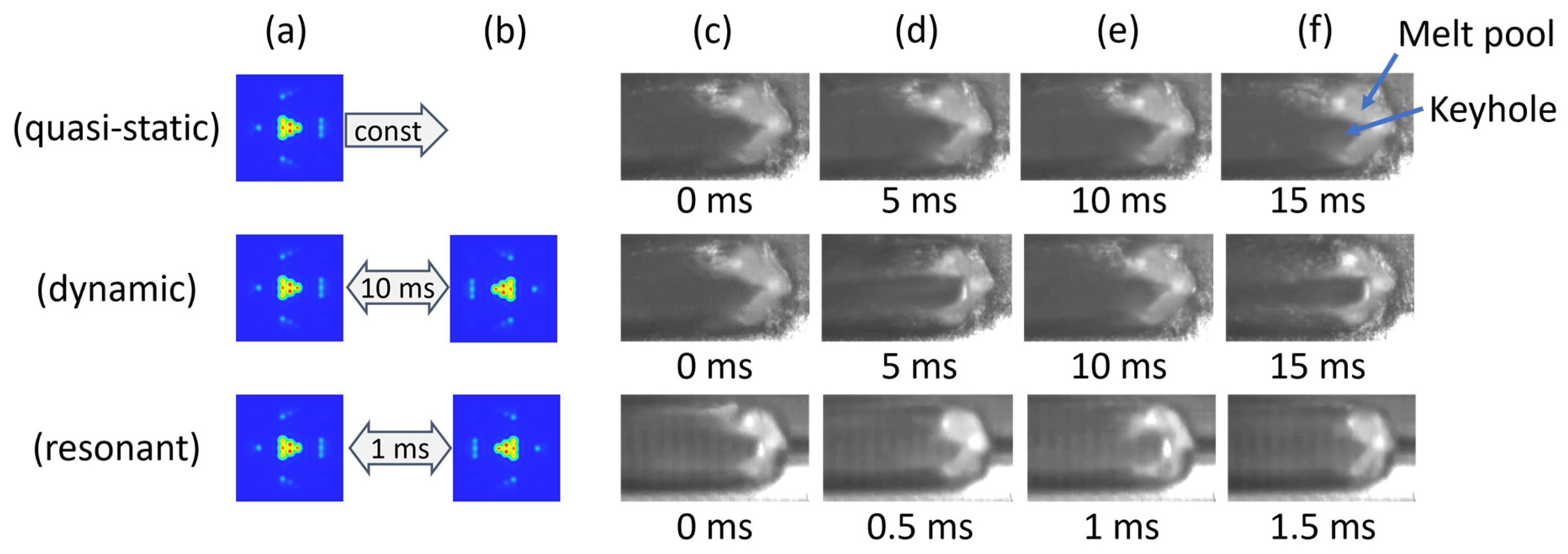
- Quasi-static beam shaping is achieved when the movement of the beam within a shape or a sequence of shapes is created in a time, which is much shorter than the relevant process time constant. In this case, the process cannot follow the movement of the laser beam or each single shape of the sequence and “sees” a temporally and spatially averaged beam shape. For the same example of keyhole welding of steel with a beam shape, which is created by a beam moving on a circle, if the circle is created in a time < 1 ms, the keyhole has about the width of the circle.
- (2)
- Dynamic beam shaping is achieved when the movement of the beam within a shape or a sequence of shapes takes place in a time that is much longer than the relevant process time constant. In this case, the process follows the movement of the laser beam or adapts to each shape of the sequence. For the example of keyhole welding of steel with a beam shape, which is created by a beam that is moving on a circle, if the circle is created in a time >1 ms, the width of the keyhole is about the width of the beam and follows the movement of the beam along the circumference of the circle. This situation is often called wobbling.
- (3)
- Resonant beam shaping is achieved when the movement of the beam within a shape or a sequence of shapes is created in a time, which is about the same as the relevant process time constant. In this case, the process might be excited by the movement of the laser beam or each single shape of the sequence.
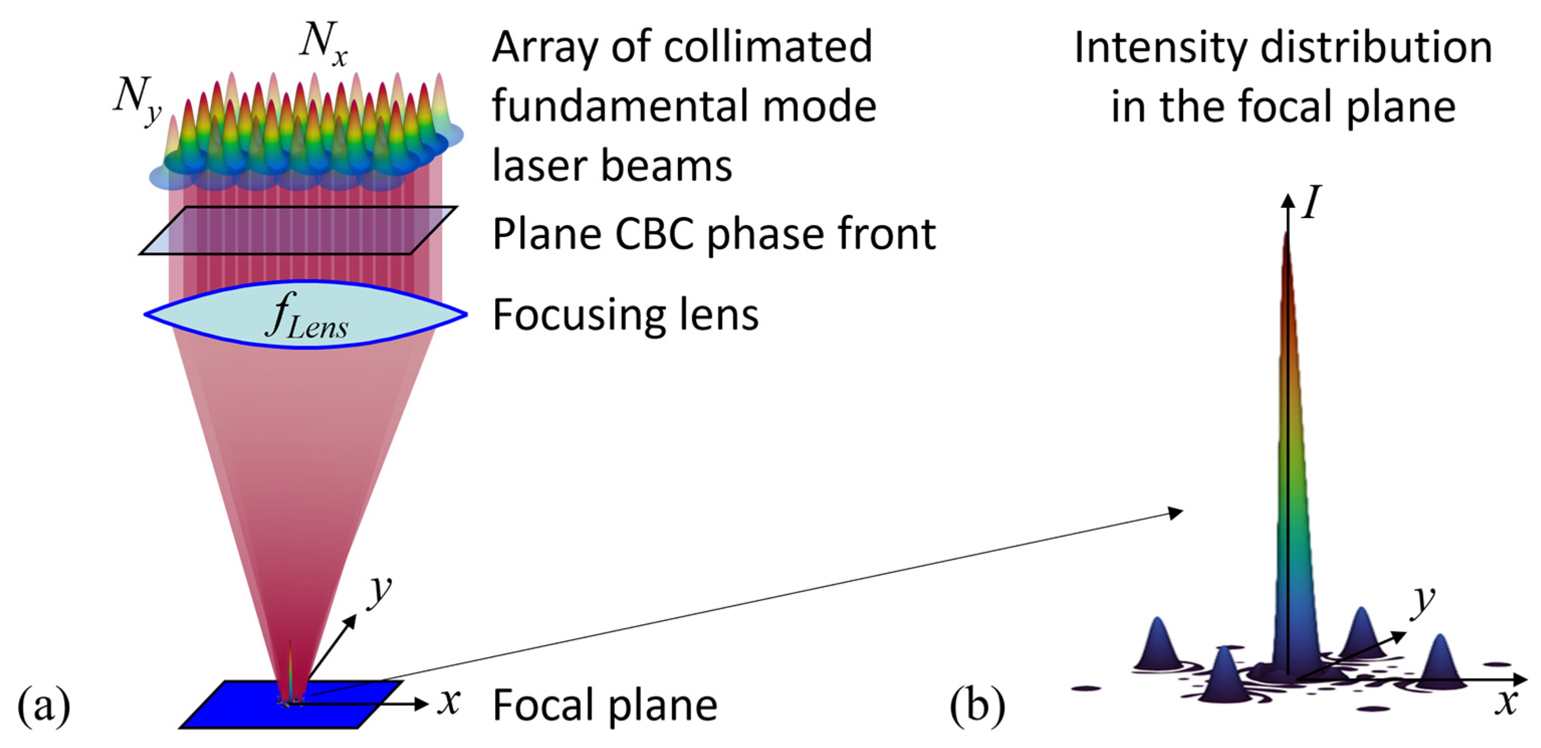
2. CBC Points
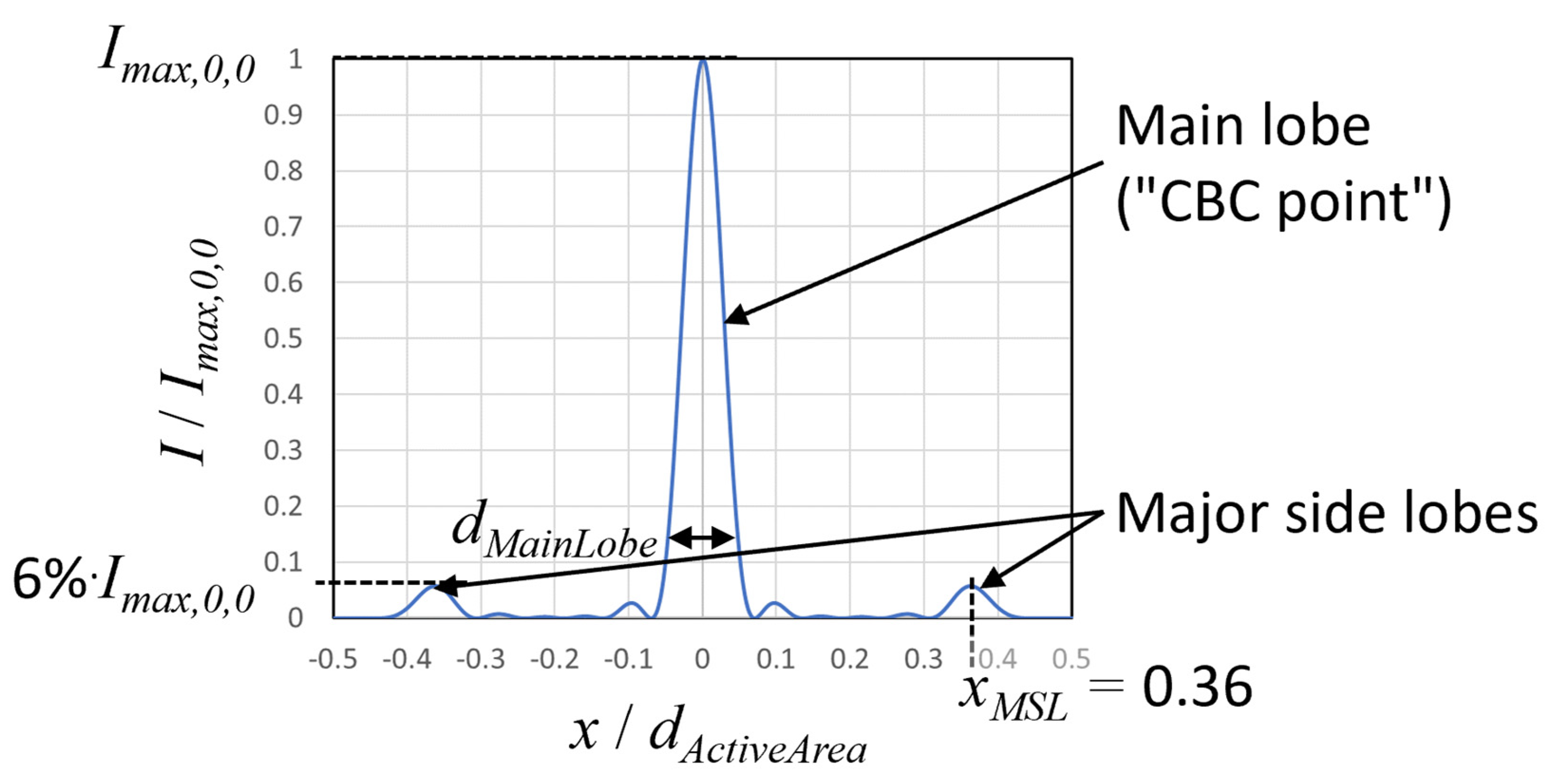
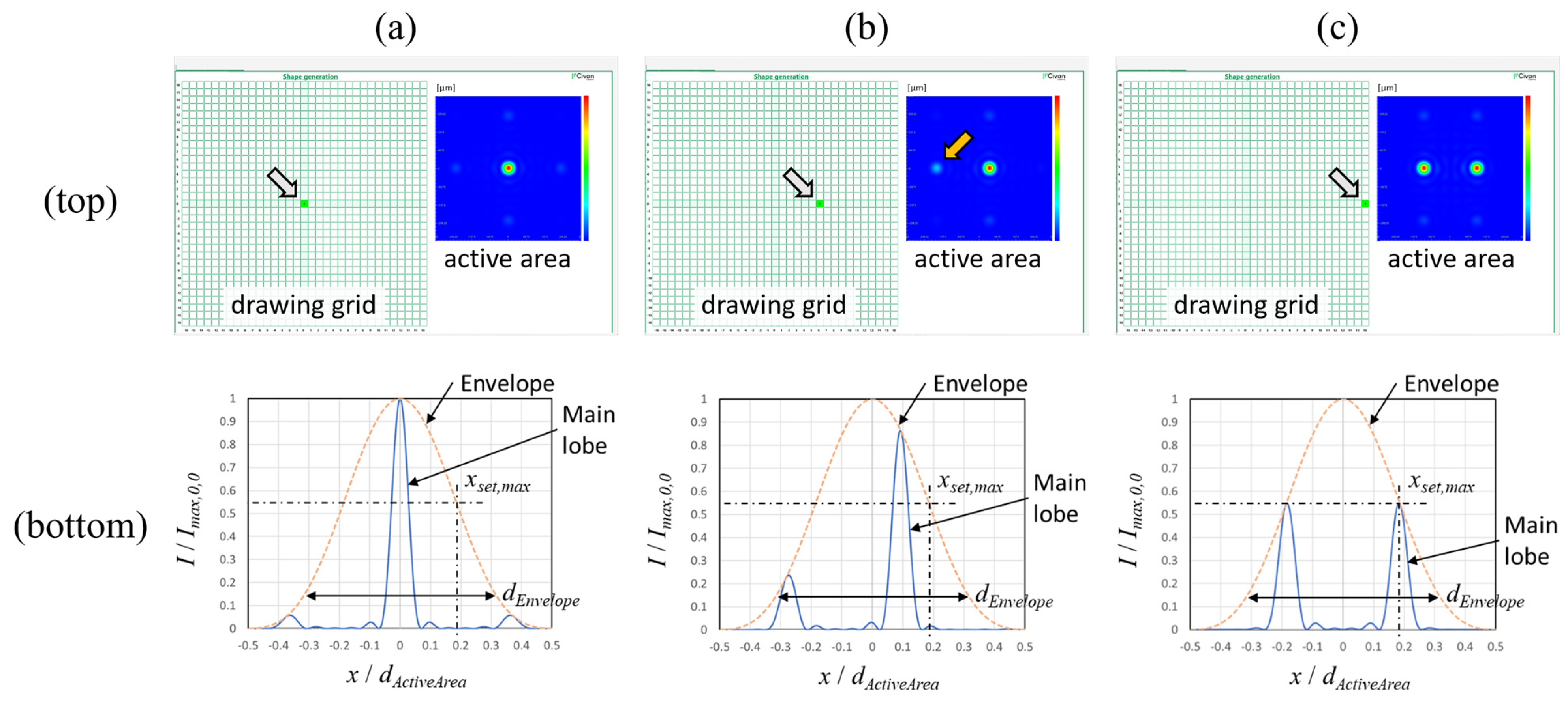
2.1. Intensity Distribution in the Focal Plane
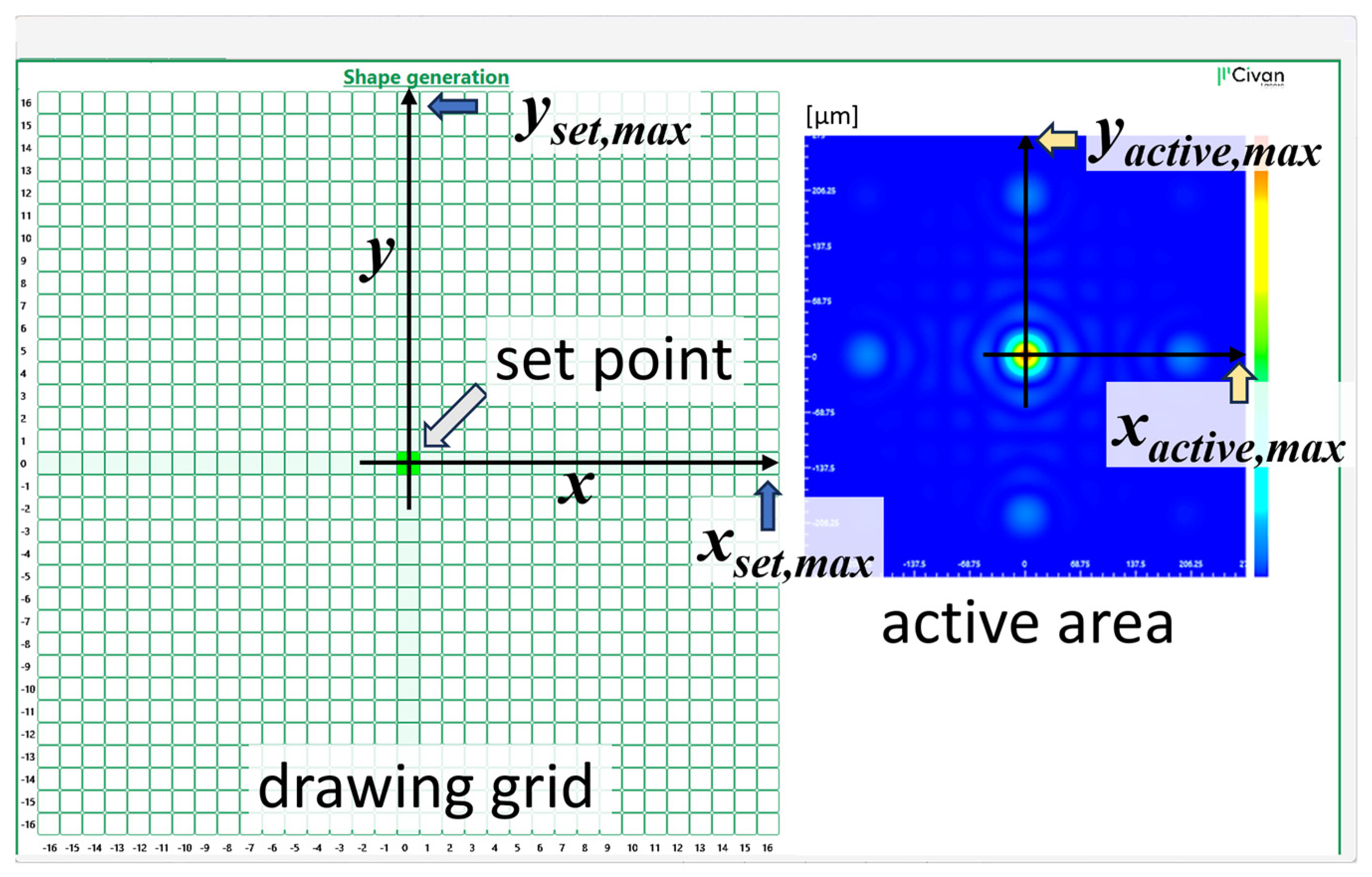
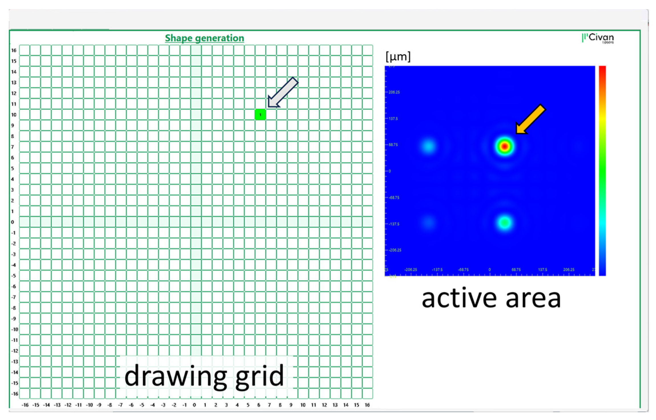
2.2. Setting Points at Arbitrary Positions
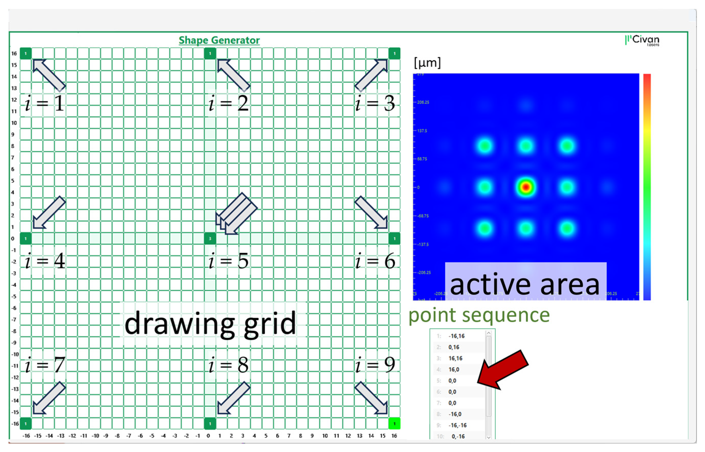
3. A Sequence of CBC Points Results in a Shape
3.1. The Principle of Shapes
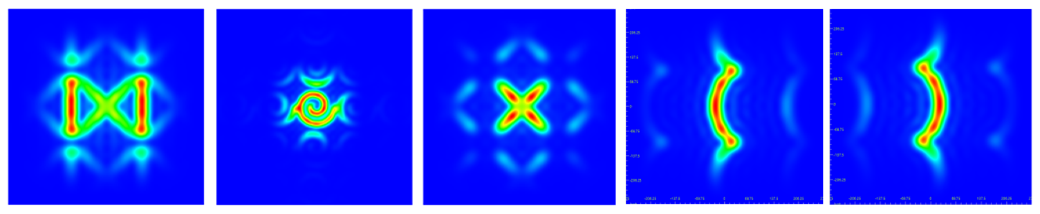
3.2. Sequences of Shapes
3.3. Depth of Focus and Active Focus Steering in z-Direction
4. Time Constants
4.1. Number of Set Positions and Number of Set Points
4.2. Shape Refresh Frequency
4.3. Shape Duration
5. Summary of the Relevant Shape Parameters
5.1. System Constraints
5.2. Definable and Resulting Shape Parameters
5.3. Comparison with Process Time Constants
- The shape refresh time of tSR = 2 μs is much shorter than the process time constant of tProc = 1 ms (tSR ≪ tProc(a)). Therefore, this is a quasi-static beam shape. The keyhole cannot follow the movement of the CBC point and adapts its shape to the beam shape.
- The shape duration of tSD =10 ms is much larger than the process time constant of tProc = 1 ms (tSD ≫ tProc(b)). This means that the process has time to dynamically adapt to each shape in the sequence of quasi-static shapes.
6. Conclusions
Author Contributions
Funding
Data Availability Statement
Conflicts of Interest
Abbreviations
| CBC | Coherent beam combining |
| OPA | Optical phased array |
| DBL | Dynamic beam laser |
| SLM | Spatial light modulator |
| DED | Directed energy deposition |
| LPBF | Laser powder bed fusion |
References
- Hügel, H.; Graf, T. Laser in der Fertigung, 5th ed.; Springer Fachmedien: Wiesbaden, Germany, 2023; ISBN 978-3-658-41122-0. [Google Scholar]
- Bocksrocker, O.; Berger, P.; Fetzer, F.; Rominger, V.; Graf, T. Local Vaporization at the Cut Front at High Laser Cutting Speeds. Lasers Manuf. Mater. Process. 2018, 24, 52006. [Google Scholar] [CrossRef]
- Hirano, K.; Fabbro, R. Possible explanations for different surface quality in laser cutting with 1 and 10 μm beams. J. Laser Appl. 2012, 24, 12006. [Google Scholar] [CrossRef]
- Eriksson, I.; Powell, J.; Kaplan, A.F.H. Melt flow measurement inside the keyhole during laser welding. In Proceedings of the 13th NOLAMP Conference: 13th Conference on Laser Materials Proce Nordic Countries, Trondheim, Norway, 27–29 June 2011. [Google Scholar]
- Fabbro, R.; Slimani, S.; Coste, F.; Briand, F. Study of keyhole behaviour for full penetration Nd–Yag CW laser welding. J. Phys. D Appl. Phys. 2005, 38, 1881–1887. [Google Scholar] [CrossRef]
- Hagenlocher, C.; Fetzer, F.; Weber, R.; Graf, T. Benefits of very high feed rates for laser beam welding of AlMgSi aluminum alloys. J. Laser Appl. 2018, 30, 012015. [Google Scholar] [CrossRef]
- Shibata, K.; Iwase, T.; Sakamoto, H.; Seto, N. Process stabilization by dual focus laser welding of aluminum alloys for car body. In Laser Processing of Advanced Materials and Laser Microtechnologies; SPIE: St. Bellingham, WA, USA, 2003. [Google Scholar] [CrossRef]
- Li, J.; Sun, Q.; Liu, Y.; Zhen, Z.; Sun, Q.; Feng, J. Melt flow and microstructural characteristics in beam oscillation superimposed laser welding of 304 stainless steel. J. Manuf. Process. 2020, 50, 629–637. [Google Scholar] [CrossRef]
- Nagel, F.; Simon, F.; Kümmel, B.; Bergmann, J.P.; Hildebrand, J. Optimization Strategies for Laser Welding High Alloy Steel Sheets. Phys. Procedia 2014, 56, 1242–1251. [Google Scholar] [CrossRef]
- Feuchtenbeiner, S.; Dubitzky, W.; Hesse, T.; Speker, N.; Haug, P.; Seebach, J.; Hermani, J.-P.; Havrilla, D. Beam shaping BrightLine Weld: Latest application results. In Proceedings Volume 10911, High-Power Laser Materials Processing: Applications, Diagnostics, and Systems VIII; 109110X; SPIE: St. Bellingham, WA, USA, 2019. [Google Scholar] [CrossRef]
- Cho, J.; Farson, D.F.; Reiter, M. Analysis of penetration depth fluctuations in single-mode fibre laser welds. J. Phys. D Appl. Phys. 2009, 42, 115501. [Google Scholar] [CrossRef]
- Heider, A.; Weber, R.; Graf, T.; Herrmann, D.; Herzog, P. Power Modulation to Stabilize Laser Welding of Copper. J. Laser Appl. 2015, 27, 022003. [Google Scholar] [CrossRef]
- Bakhtari, A.R.; Sezer, H.K.; Canyurt, O.E.; Eren, O.; Shah, M.; Marimuthu, S. A Review on Laser Beam Shaping Application in Laser-Powder Bed Fusion. Adv. Eng. Mater. 2024, 26, 2302013. [Google Scholar] [CrossRef]
- Bayat, M.; Rothfelder, R.; Schwarzkopf, K.; Zinoviev, A.; Zinovieva, O.; Spurk, C.; Hummel, M.; Olowinsky, A.; Beckmann, F.; Schmidt, J.M.M.; et al. Exploring spatial beam shaping in laser powder bed fusion: High-fidelity simulation and in-situ monitoring. Addit. Manuf. 2024, 93, 104420. [Google Scholar] [CrossRef]
- Schmidt, M.; Cvecek, K.; Duflou, J.; Vollertsen, F.; Arnold, C.B.; Matthews, M.J. Dynamic beam shaping—Improving laser materials processing via feature synchronous energy coupling. CIRP Ann. 2024, 73, 533–559. [Google Scholar] [CrossRef]
- Cronin-Golomb, M.; Yariv, A.; Ury, I. Coherent coupling of diode lasers by phase conjugation. Appl. Phys. Lett. 1986, 48, 1240. [Google Scholar] [CrossRef]
- Müller, M.; Aleshire, C.; Klenke, A.; Haddad, E.; Légaré, F.; Tünnermann, A.; Limpert, J. 3.5 kW coherently combined ultrafast fiber laser. Opt. Lett. 2018, 43, 6037–6040. [Google Scholar] [CrossRef] [PubMed]
- Müller, M.; Klenke, A.; Steinkopff, A.; Stark, H.; Tünnermann, A.; Limpert, J. 10.4 kW coherently combined ultrafast fiber laser. Opt. Lett. 2020, 45, 3083–3086. [Google Scholar] [CrossRef] [PubMed]
- Fan, T.Y. Laser beam combining for high-power, high-radiance sources. IEEE J. Sel. Top. Quantum Electron. 2005, 11, 567–577. [Google Scholar] [CrossRef]
- Shekel, E.; Vidne, Y.; Urbach, B. 16 kW single mode CW laser with dynamic beam for material processing. In Fiber Lasers XVII: Technology and Systems; SPIE: St. Bellingham, WA, USA, 2020; p. 73. [Google Scholar] [CrossRef]
- Nissenbaum, A.; Armon, N.; Shekel, E. Dynamic beam lasers based on coherent beam combining. In Proceedings Volume 11981, Fiber Lasers XIX: Technology and Systems; 119810B; SPIE: St. Bellingham, WA, USA, 2022. [Google Scholar] [CrossRef]
- Kuang, Z.; Li, J.; Edwardson, S.; Perrie, W.; Liu, D.; Dearden, G. Ultrafast laser beam shaping for material processing at imaging plane by geometric masks using a spatial light modulator. Opt. Lasers Eng. 2015, 70, 1–5. [Google Scholar] [CrossRef]
- Wagner, J.; Heider, A.; Ramsayer, R.; Weber, R.; Faure, F.; Leis, A.; Armon, N.; Susi, R.; Tsiony, O.; Shekel, E.; et al. Influence of dynamic beam shaping on the geometry of the keyhole during. In Proceedings of the LANE 2022, Fürth, Germany, 4–8 September 2022. [Google Scholar]
- Sawannia, M.; Wagner, J.; Stritt, P.; Ramsayer, R.; Hagenlocher, C.; Graf, T. Response of the melt pool and vapour capillary on dynamic beam shaping in the kHz regime during laser welding. In Proceedings of the LANE 2024, Fürth, Germany, 15–19 September 2024. [Google Scholar]
- Zhao, C.; Parab, N.D.; Li, X.; Fezza, K.; Tan, W.; Rollett, A.D.; Sun, T. Critical instability at moving keyhole tip generates porosity in laser melting. Science 2020, 370, 1080–1086. [Google Scholar] [CrossRef] [PubMed]
- Bernhard, R.; Assa, R.; Armon, N.; Shekel, E. Tailored beamshape sequences for welding using a Dynamic Beam Laser. Procedia CIRP 2024, 124, 730–732. [Google Scholar] [CrossRef]

| fLens (m) | dMainLobe (μm) | Imax,0,0 (W/cm2) | xset,max (μm) | xactive,max (μm) | dActiveArea (μm) |
|---|---|---|---|---|---|
| 0.75 | 68 | 3.9 × 10⁸ | 130 | 356 | 712 |
| 1.0 | 91 | 2.2 × 10⁸ | 173 | 474 | 949 |
| 1.5 | 136 | 9.8 × 10⁷ | 259 | 712 | 1423 |
| 3.0 | 273 | 2.5 × 10⁷ | 518 | 1423 | 2847 |
| fLens (m) | Depth of Focus ∆zFocus (mm) | Active Focus Steering ∆zSteering (mm) |
|---|---|---|
| 0.75 | ±2.9 | ±7.2 |
| 1.0 | ±5.1 | ±12.8 |
| 1.5 | ±11.5 | ±28.9 |
| 3.0 | ±45.9 | ±115.4 |
| Item | Symbol | Example Limits DBL 6–14 kW |
|---|---|---|
| Maximum OPA modulation frequency | fOPA,max | 80 MHz |
| ⇨ Shortest possible lifetime of one point | tSP,min = 1/fOPA,max | 12.5 ns |
| Maximum total number of points in a shape | NSP,max | 1024 |
| Maximum number of shapes in a sequence | NShapes,max | 14 |
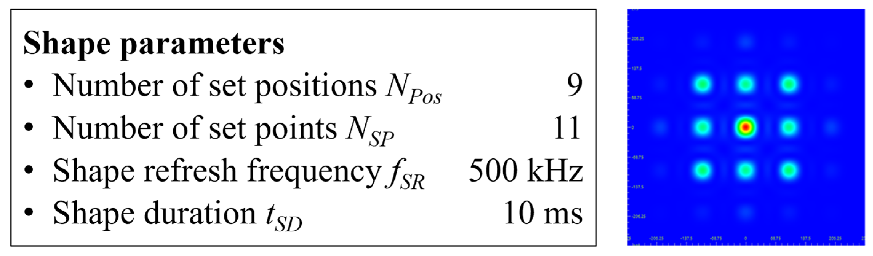
| Item | Symbol | Example 7 |
|---|---|---|
| Total number of positions in the shape | NPos | 9 |
| Number of set points at the ith position | NC,i | 1 (i ≠ 5) 3 (i = 5) |
| Total number of points in the shape | 11 | |
| Shape refresh frequency | fSR | 500 kHz |
| ⇨ Duration for drawing the complete shape | tSR = 1/fSR | 2 μs |
| ⇨ Lifetime of one single CBC point | tSP = tSR/NSP | 181.8 ns |
| ⇨ Point frequency in the shape | fP = 1/tSP = NSP/tSR = NSP × fSR | 5.5 MHz |
| ⇨ Dwell time at the ith position | tDwell,i = NC,i × tSP | 181.8 ns (i ≠ 5) 545.4 ns (i = 5) |
| Duration of the shape (persistence) | tSD | 10 ms |
| ⇨ Shape duration frequency | fSD = 1/tSD | 100 Hz |
| ⇨ The shape is drawn NS times per duration | NS = tSD × fSR | 5000 |
| Quasi-Static Beam Shaping | |||
|---|---|---|---|
| Shape Parameter | Frequency | Time | Resulting Effect in the Process |
| Shape refresh | fSR ≫ fProc | tSR ≪ tProc (a) | The process adapts to the shape (required for each shape in a sequence) |
| Shape duration | fSD ≫ fProc | tSD ≪ tProc | The process adapts to an average of all shapes in the sequence (“average shape”) |
| Dynamic beam shaping | |||
| Shape parameter | Frequency | Time | Resulting effect in the process |
| Shape refresh | fSR ≪ fProc | tSR ≫ tProc | The process follows the diffraction pattern (“moving beam”, “wobbling”) |
| Shape duration | fSD ≪ fProc | tSD ≫ tProc (b) | The process adapts to each shape in a sequence (the shapes must be quasi-static) |
| Resonant beam shaping | |||
| Shape parameter | Frequency | Time | Resulting effect in the process |
| Shape refresh | fSR ≈ fProc | tSR ≈ tProc | The beam excites the process resonantly (“resonant stirring”) |
| Shape duration | fSD ≈ fProc | tSD ≈ tProc | The shape sequence excites the process resonantly (“resonant shaking”) |
Disclaimer/Publisher’s Note: The statements, opinions and data contained in all publications are solely those of the individual author(s) and contributor(s) and not of MDPI and/or the editor(s). MDPI and/or the editor(s) disclaim responsibility for any injury to people or property resulting from any ideas, methods, instructions or products referred to in the content. |
© 2025 by the authors. Licensee MDPI, Basel, Switzerland. This article is an open access article distributed under the terms and conditions of the Creative Commons Attribution (CC BY) license (https://creativecommons.org/licenses/by/4.0/).
Share and Cite
Weber, R.; Wagner, J.; Peter, A.; Hagenlocher, C.; Spira, A.; Urbach, B.; Shekel, E.; Vidne, Y. Basic Properties of High-Dynamic Beam Shaping with Coherent Combining of High-Power Laser Beams for Materials Processing. J. Manuf. Mater. Process. 2025, 9, 85. https://doi.org/10.3390/jmmp9030085
Weber R, Wagner J, Peter A, Hagenlocher C, Spira A, Urbach B, Shekel E, Vidne Y. Basic Properties of High-Dynamic Beam Shaping with Coherent Combining of High-Power Laser Beams for Materials Processing. Journal of Manufacturing and Materials Processing. 2025; 9(3):85. https://doi.org/10.3390/jmmp9030085
Chicago/Turabian StyleWeber, Rudolf, Jonas Wagner, Alexander Peter, Christian Hagenlocher, Ami Spira, Benayahu Urbach, Eyal Shekel, and Yaniv Vidne. 2025. "Basic Properties of High-Dynamic Beam Shaping with Coherent Combining of High-Power Laser Beams for Materials Processing" Journal of Manufacturing and Materials Processing 9, no. 3: 85. https://doi.org/10.3390/jmmp9030085
APA StyleWeber, R., Wagner, J., Peter, A., Hagenlocher, C., Spira, A., Urbach, B., Shekel, E., & Vidne, Y. (2025). Basic Properties of High-Dynamic Beam Shaping with Coherent Combining of High-Power Laser Beams for Materials Processing. Journal of Manufacturing and Materials Processing, 9(3), 85. https://doi.org/10.3390/jmmp9030085