Abstract
Short fiber reinforced thermoplastics (SFT) are extensively used due to their excellent mechanical properties and low processing costs. Long fiber reinforced thermoplastics (LFT) show an even more interesting property profile and are increasingly used for structural parts. However, their processing by injection molding is not as simple as for SFT, and their anisotropic properties resulting from the fiber microstructure (fiber orientation, length, and concentration) pose a challenge with regard to the engineering design process. To reliably predict the structural mechanical properties of fiber reinforced thermoplastics by means of micromechanical models, it is also necessary to reliable predict the fiber microstructure. Therefore, it is crucial to calibrate the underlying prediction models, such as the fiber orientation model, within the process simulation. In general, these models may be adjusted manually, but this is usually ineffective and time-consuming. To overcome this challenge, a new calibration method was developed to automatically calibrate the fiber orientation model parameters of the injection molding simulation by means of optimization methods. This optimization routine is based on experimentally determined fiber orientation distributions and leads to optimized parameters for the fiber orientation prediction model within a few minutes. To better understand the influence of the model parameters, different versions of the fiber orientation model, as well as process and material influences on the resulting fiber orientation distribution, were investigated. Finally, the developed approach to calibrate the fiber orientation model was compared with a classical approach, a direct optimization of the whole process simulation. Thereby, the new optimization approach shows a calculation time reduced by the factor 15 with comparable error variance.
1. Introduction
Due to the ever-decreasing development times and the steady progress of digitization, numerical methods for predicting unknown target and design variables are gaining in importance. This also applies to the processing of plastics and the resulting part properties in general. Especially in the case of fiber-reinforced plastics, the strongly varying part properties directly depend on the fiber microstructure and must be taken into account during the design process [1,2,3,4]. In the following, the fiber microstructure is used as a generic term for fiber orientation, fiber length, and fiber concentration.
A reliable prediction of the process-induced fiber microstructure, especially for long fiber reinforced thermoplastics (LFT), still poses a considerable challenge today [5,6,7]. In contrast to short fiber reinforced thermoplastics (SFT), not only the fiber orientation must be taken into account in the prediction of the mechanical properties of LFTs, but effects such as fiber breakage and the migration of fibers during processing also play a significant role. In order to predict these properties correctly, suitable calculation models are required on the one hand, and correspondingly well-calibrated model parameters on the other hand.
However, the reliable prediction of fiber orientation in general, but especially for LFTs, is still the subject of current research and requires further improvement in the achievable prediction quality. Current commercial software environments that calculate the injection molding process do not allow a purposeful and fast optimization of the resulting fiber orientation distribution. Only a manual adaptation of model parameters with a subsequent recalculation of the entire flow field is possible. Due to the lack of automation and the necessary recalculations, the calibration of the model parameters becomes remarkably inefficient and time-consuming. Therefore, a new calibration method was developed to automatically adjust the resulting fiber orientation distribution.
1.1. State of the Art
During the processing of discontinuous fiber reinforced plastics, a specific fiber microstructure (fiber orientation, fiber length and fiber concentration) is formed within the part cavity that depends on the material, the geometry of the molded part, and the process settings. This microstructure determines the parts main properties. With suitable accuracy of the predicted fiber microstructure the resulting anisotropic mechanical properties can be reliably calculated [8,9,10,11,12]. Thus, the part’s behavior can also be determined in structural simulations.
1.1.1. Fiber Microstructure
The resulting part properties of fiber reinforced materials are mainly determined by process induced fiber microstructure and its properties (Figure 1), such as:

Figure 1.
Influence of fiber orientation, length, and concentration on the resulting mechanical properties (schematically) according to [16,26,29].
- fiber orientation [13,14,15,16,17,18,19,20,21,22],
- fiber length and diameter [10,20,23,24,25,26,27,28],
- fiber concentration [10,23,29], and
- fiber matrix adhesion [29,30].
The increase in the respective fiber microstructure properties (orientation, length, and concentration) also leads to an increase in mechanical properties of the composite material, such as stiffness, strength, and impact strength [23]. Only at high fiber concentrations can a decrease in strength and impact strength be observed. With regard to an entire fiber reinforced part, the local distribution of these properties along the flow path as well as along the cavity height (part thickness) must also be taken into account [31]. Even if in some cases a classification cannot be clearly distinguished, fiber reinforced materials are categorized into three classes according to their initial or resulting fiber length [32]: short fiber reinforced plastics (0.1–1 mm), long fiber reinforced plastics (1–50 mm), and continuous fiber reinforced plastics (>50 mm).
1.1.2. Process Induced Microstructure
The properties of the fiber microstructure (orientation, length, and concentration), especially in the case of discontinuously reinforced plastics such as SFT or LFT, can usually only be influenced to a very limited extent by its constituent properties and compound constitution (initial fiber orientation, initial fiber length and initial fiber concentration). However, these properties are rather a result of the processing [13,26,33,34,35,36,37]. One of the most widely used processing methods is injection molding, in which even complex parts can be produced in large quantities [32,37].
The materials used are subjected to special stresses during the injection molding process. This can be seen in the orientation of the fibers as well as in the migration and fracture phenomena. During the filling of a part with molten plastic by injection molding, a flow field is formed inside the cavity that depends on the material, the part geometry, and the process settings. This varies not only along the flow direction, for example through cooling effects, but also along the part’s thickness or the cavity height, as shown in Figure 2. Due to this velocity profile and the resulting shear stresses, characteristic layers are formed along the part thickness (Figure 3) in which the fibers
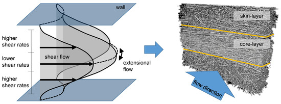
Figure 2.
Velocity profile and the resulting fiber orientation distribution according to [51].

Figure 3.
Locally varying fiber microstructure along the normalized part thickness (schematically).
- are aligned differently (fiber orientation) [31,38,39,40,41,42,43,44,45],
- break more frequently (fiber length) [43,46,47,48], or
- migrate unevenly (fiber concentration) [5,14,45,49,50].
These individual microstructure properties also affect each other. Due to the interaction of the fibers, the fiber orientation depends on the fiber length and concentration [5], which also applies to interchanged dependencies. The fiber length depends on the fiber orientation and concentration while the distribution of fibers depends inversely on the fiber orientation and length [36]. Due to wall adhesion and mold cooling, high shear rates are present in the skin or shear layers, and lower shear rates are found in the core layer in the middle of the cavity. A characteristic profile for each property is created inside a part, which can be subdivided into different layers [38,41,52] as shown in Figure 3.
According to the crystalline structure [34,53] or the fiber orientation distribution [46,54], the flow profile can be divided into at least a core layer and two shear or skin layers. This three-layer model is shown schematically in Figure 2 (right), and the individual microstructure properties are shown in Figure 3. The specific characteristic ratio of the layers is determined by the quotient of the individual layer thicknesses and is generally referred to as the skin core layer ratio.
The influence of the velocity field on the resulting fiber orientation distribution is a complex interrelation. The flow field changes in response to many different influencing factors. Important parameters are, for example, the injection speed and the processing temperature, as well as the material’s viscosity [14]. Figure 4 shows the correlation of the shear rate and injection speed [55] along the cavity height.

Figure 4.
Influence of the injection speed on the velocity profile according to [55].
At high injection speeds (Figure 4b), the maximum shear rate shifts towards the mold wall, and the core layer width increases [39]. Whereas, for lower injection speeds (Figure 4a) the maximum of the shear rate profile shifts towards the cavity core, the range of the high shear rates generally increases, and the core layer width decreases. Depending on the shear and extensional flow inside the cavity, individual layers are formed with their associated fiber orientation distribution [19].
Furthermore, the viscosity of the melt changes with the type of matrix polymer and the reinforcing filler material (material, geometry, concentration, length, diameter, orientation, adhesion etc.) [42] as shown in Figure 5a. For example, a higher fiber concentration results in a higher viscosity, which leads to a different velocity and shear rate profile, as shown in Figure 5b,c [32,56]. In areas of low shear rates in particular, the viscosity of filled polymers differs strongly from that of unfilled polymers. Higher fiber concentrations mostly result in smaller skin layers due to their shear thinning behavior [19,39,57,58]. For this reason, different viscosity models are required to describe specific material behavior at low shear rates for reinforced or filled polymers (Figure 5b). For injection molding simulation, a frequently used model was developed by Herschel and Bulkley. A detailed description of the Herschel–Bulkley model is given in Section 1.1.7.
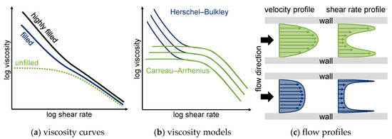
Figure 5.
Influence of the viscosity to the velocity profile according to [59].
1.1.3. Fiber Orientation Distribution of Short and Long Fiber Reinforced Thermoplastics
As mentioned before, the properties of the reinforcement itself and the fiber microstructure properties also affect each other. In this context, the resulting fiber length inside a part plays a crucial role in the resulting fiber orientation [1]. The fiber length in particular causes a varying layer ratio, which can be seen in the fiber orientation distribution of short and long fiber reinforced plastic parts [39,44]. Even if the fiber breakage and the resulting fiber length are also determined by its orientation inside the flow, the resulting fiber orientation is more dominated by the fiber length. As Figure 6 schematically demonstrates, the degree of orientation in the skin layer decreases and the core layer width increases with increased fiber length [39,44,47,54]. Furthermore, in some cases, the degree of fiber orientation perpendicular to the flow direction () in the core layer can also exceed the degree of fiber orientation parallel to the flow direction (), as shown in Figure 6b, for a long fiber reinforced plastic. In that special case, the mechanical properties perpendicular to the flow can also exceed the mechanical properties in the direction of flow.
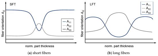
Figure 6.
Characteristic fiber orientation distributions along the parts thickness in discontinuous fiber reinforced plastics.
1.1.4. Tensorial Description of the Fiber Orientation
The fiber orientation is usually described as a 2nd order orientation tensor according to Advani and Tucker [60]. The tensor describes the orientation of all fibers in a defined volume or element where is a probability density function, which is a statistical description of orientation states. The orientation tensor is calculated as an integral over all possible fiber orientations from the distribution function of the fibers and the dyadic product of the unit vectors . The first entry describes the orientation of the fibers in the flow direction and is represented in Figure 7a. The eigenvectors of the tensor indicate the principal direction of fiber orientation, while the eigenvalues indicate the degree of fiber orientation, i.e., the statistical proportion of fibers in the respective principal direction.
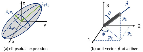
Figure 7.
Tensorial Description of the Fiber Orientation.
The calculation of fiber orientation is based on a previously computed flow field. The velocity gradient tensor and the shear rate are required as input variables. The result is a tensor that describes the orientation of the fibers in the melt or flow channel in three dimensions [60].
The diagonal entries , and describe the orientation in the three spatial directions.
1.1.5. Experimental Determination of the Fiber Orientation
Several methods have been developed to analyze the fiber microstructure, such as ultrasound methods [61,62], optical methods like grinding pattern analysis [35,40,60,63,64,65,66,67,68,69,70], electron microscopy [14], Radiography [45,71,72] and X-ray computed tomography (CT) [73,74,75,76,77,78]. However, all methods are usually associated with high effort and are therefore used infrequently. To determine the spatial fiber orientation by means of cross section analysis, each fiber ellipsis, as shown in Figure 8a, has to be measured by its major and minor axis according to Figure 8b. With the trigonometric functions depicted in Figure 8c, the fiber orientation tensor components can be calculated for each fiber [40,60]. In addition, the reduced cutting probabilities of the inclined fibers can be considered by applying a weighting function according to [40,79].

Figure 8.
Cross section analysis to experimentally determine fiber orientation.
1.1.6. Injection Molding Simulation
For the simulation of the unsteady, non-Newtonian and non-isothermal injection molding process, the three-dimensional basic Equations for fluid mechanics are usually solved using the finite volume method (FVM). The basic equations for conservation of mass (2), conservation of linear momentum (3), and energy (4), are solved by FVM numerically [16,80].
conservation of mass:
conservation of momentum:
conservation of energy:
Based on these three equations, flow velocities and their gradients are calculated, which represent the major determining variables for the subsequent fiber orientation calculation. The velocity gradient tensor describes the change of velocity in the three spatial directions of a stationary flow and can be split into a symmetrical and a rotational component (Equation (5)). From the deformation velocity tensor , the shear rate can be derived (Equation (6)). However, for a detailed description of the FVM for injection molding simulation, refer to [80].
1.1.7. Viscosity Models
To describe the flow behavior of plastic melts [81], several different viscosity models were developed. The Herschel–Bulkley model is frequently used to accurately represent the viscosity of long fiber reinforced thermoplastics especially in the range of low shear rates. In this model, on the one hand, the yield stress viscosity at low shear rates is considered, which can be determined experimentally by rotational rheometry [82,83]. On the other hand, the range of high shear rates is precisely covered where so-called shear thinning [84] is present. This range can experimentally be determined by means of capillary rheometry. The model is composed of the Herschel–Bulkley yield stress (first term) and the Cross-WLF viscosity (second term), as shown in Equation (7) with power-law index , temperature , pressure , and zero shear viscosity η0.
The model consists of seven parameters , , , , , , and in order to approximate the shear rate distribution of the materials viscosity.
1.1.8. Fiber Orientation Models
To calculate fiber orientation distributions, the tensorial description developed by Advani and Tucker [60] is usually used. The corresponding calculation models are mostly based on the extension of the Jeffery model [85] made by Folgar and Tucker [86]. Current commercial injection molding solvers also use combined model extensions, such as the RPR (retarding principal rate) and ARD or iARD (improved anisotropy rotary diffusion) models. The iARD-RPR model is a combination of Jeffery’s hydrodynamic model (HD), the extension of the IRD model (isotropic rotary diffusion) from Folgar–Tucker to the iARD model and the RPR model (Equation (12)), according to Tseng et al. [87,88,89]. With (fiber–fiber interaction coefficient), (fiber–matrix interaction coefficient), and (slow-down parameter), a changing of the fiber orientation based on the existing flow field can be calculated. The influencing factors of the calculated fiber orientation are in this case the gradient tensor and the shear rate of the flow field.
This leaves three model parameters , , and , which can be used to adjust or calibrate the fiber orientation distribution. The first part is defined as iARD (Equation (9)) [87].
In addition to the second order orientation tensor, the fourth order orientation tensor is required for the calculation, and is solved with invariant-based closure approximation (IBOF5) according to Chung and Kwon [90], which is a model that offers a good compromise of a precise approximation and computation effort.
The rotary diffusion tensor (Equation (11)) is determined by the scalar (Equation (10)) of the square of the symmetrical part from the velocity gradient tensor .
The second part describes the retarded principal rate (Equation (12))
with ΛIOK (Intrinsic Orientation Kinetics), as the substantial derivative of a certain diagonal tensor. In general, an eigenvalue calculation of both the orientation tensor and its change is coupled here. This is realized as follows (Equations (13) and (14)):
where represents the eigenvalues of the orientation tensor and the rotation matrix, which is composed of the eigenvectors of the change in the orientation tensor. This relationship is extended as follows (Equation (15))
with an additional parameter β, which is defined as a time constant.
In order to determine the different influences of the velocity field more precisely, the parameters and were calculated depending on the shear rate according to Tseng et al. [91]. Figure 9 shows that was adjusted in the core layers, which damps this parameter at lower shear rates, while the opposite is true for , which is damped at higher shear rates.

Figure 9.
Shear rate-dependent adaption of the parameters and [91].
For this purpose, the parameters are changed as follows (Equations (16) and (17)) [91].
The and input values are given by the user and then changed to a specific value for each element of the simulation model. With , a critical shear rate is defined, which has to be determined empirically. In commercial simulation tools like Moldex3D® R17 this variable is implemented as a constant determined by experience of the developers.
1.1.9. Calibration of Fiber Orientation Models
The model parameters play a crucial role in the use of fiber orientation models, because only with an appropriately calibrated model the fiber orientation can be reliably predicted [7,40,88,92,93,94]. The main challenge here is that the model parameters are not exclusively material-dependent, but may even depend on the process and part geometry [94,95]. Therefore, standard parameters can only be used rarely or only for a few specific cases. Especially for LFTs, a reliable prediction with current models is not possible when using standard parameters.
Most publications concerning the prediction of fiber orientation either use standard parameters [2] or simply adjust or fine tune them manually by trial and error [1,96]. Sometimes there is a so-called fit, but no algorithm for the parameter identification is described [8,88,92,97,98]. Independently of the geometry, objective fitting methods has been described for simple shear flows of short fiber [99] and also long fiber [100] reinforced plastics. Some of the necessary model parameters like the fiber-fiber interaction coefficient were extensively analyzed and associated approximation functions [95,101,102] were developed, respectively. The influence of the parameters of recent fiber orientation models [87,92,103,104] or viscosity [6,105] has been investigated in some publications, but basic correlations to the material or approximated functions to evaluate the model parameters are still missing.
Several methods are available to optimize the necessary parameters of the prediction models for the microstructure of fiber reinforced plastics. In a first step, however, the properties of the microstructure must be determined, or methods as described in Section 3.2 must be developed in order to compare certain properties with each other directly [106]. Scalar values, such as the spatial fiber concentration, are less problematic than the fiber orientation and length, which are subject to a certain distribution even in local areas. If these requirements are satisfied, the parameters of the respective prediction models can be optimized by means of a reverse engineering procedure, as shown in Figure 10. However, even though it is possible to automatically optimize the parameters of the fiber orientation model, only a few algorithms are described in the literature [94,106,107,108,109].

Figure 10.
Reverse engineering of fiber microstructure properties at a specific position.
1.1.10. Optimization Methods
The aim of this study is to predict the experimentally determined fiber orientation with minimum error variance by optimizing the parameters of the fiber orientation model (, , and for example for the iARD model, see Section 1.1.8). According to the previous Section 1.1.9, the most suitable calibration of the fiber orientation model should be identified. Since the intention of this work is not the invention of an improved optimization algorithm, the basics of optimization methods will only be described in principle. A detailed description and a comparison of different approaches to optimization will be omitted and reference will be made to further literature [110,111].
In general, parameter optimization deals with the problem of finding a parameter vector for which a given target function is minimized. Non-linear variation methods of the form are solved. This function can be approximated by quadratic Taylor series approximation Equation (18).
where represents the gradient of , and represents the Hessian matrix of . The gradient of is calculated as follows by finding the minimum of the gradient (Equation (19))
For the use of the Newton method for problems with constraints, an additional state variable is added to the original Equation, which leads to the following variation Equation (20).
In order to determine , various line search techniques or methods can be used to directly satisfy the decisive variable constraints. In addition, the Hessian matrix can be approximated by a diagonal matrix This simplifies the optimization to a quasi-Newton method [112,113].
1.2. Objectives and Hypotheses
According to the major challenge to reliably predict the behavior of discontinuously fiber reinforced parts produced by injection molding, a holistic approach to predict all considerable properties of the fiber microstructure is desirable. In a first step, the following hypotheses are drawn and investigated to improve the predicted fiber orientation. In the future, these investigations can be extended to the remaining microstructural properties such as fiber length and fiber concentration.
On the one hand, the prediction accuracy of the fiber orientation distribution can be significantly improved by using optimization methods. On the other hand, the required optimization time can be significantly reduced with a new calibration approach.
In order to optimize the parameters of the fiber orientation model to predict the experimentally determined fiber orientation with a minimum error variance, two different calibration approaches are investigated. However, since there have been several further developments of the iARD fiber orientation model in the last few years; the most suitable version is initially identified. In the first calibration approach, a commercial simulation software is used to calculate the fiber orientation model, and only the parameters of the fiber orientation model are externally optimized in another tool to obtain the most accurate prediction for the fiber orientation distribution. As second approach, a new method is developed to calibrate the fiber orientation model. The aim of the new approach is to achieve the optimization goal as quickly and efficiently as possible. Therefore, in contrast to the first approach, which requires a time-consuming recalculation of the entire flow field with each optimization step, the new approach is based on only one initial calculation of the flow field. The subsequent parameter optimization of the fiber orientation model is performed without any further calculation of the flow field. With this approach, a suitable calibration of the fiber orientation model should be achieved within a few minutes.
Even though the new approach focuses on the calibration of the fiber orientation model, the method should be designed in a way that it can be easily transferred to other models to predict microstructural properties. For example, in the future, this approach should also be used to calibrate the models to predict fiber length and fiber concentration.
2. Experimental Setup
2.1. Materials, Parts, and Processing
The fiber orientation distribution was experimentally determined for injection molded plates according to ISO 294-5 with dimensions of 80 × 80 × 4 mm, as shown in Figure 11a.
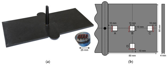
Figure 11.
Injection molded plates (a) and scheme of evaluation points along one side of the plate (b).
A long fiber reinforced polypropylene (PP-LGF) from TechnoCompound GmbH, Bad Sobernheim, Germany was chosen, because it is the most frequently used LFT material [114]. The granules are 10 mm long, rod-shaped pellets with fiber mass fractions of 20%, 40%, and 60% of the product type TechnoFiber. The plates were injection molded with two constant injection speeds of 30 cm3/s (low) and 100 cm3/s (high), a melt temperature of 230 °C and a mold temperature of 80 °C on an injection molding machine, Allrounder 520S 1600–400 from Arburg, Lossburg, Germany.
For the experimental determination of the fiber orientation distribution, small samples (10 mm × 10 mm) were taken at the beginning (A), middle (B), end (C) and aside (D) of the flow path according to Figure 11b. These samples were analyzed by inspecting the cross sections highlighted with red in Figure 11, using optical reflection microscopy as described in the following section.
2.2. Experimental Determination of the Fiber Orientation Distribution
With the image processing program FIJI (ImageJ), developed by Wayne Rasband, in combination with MATLAB® by MathWorks®, Natick, USA, spatial fiber orientation for the individual cross section were determined using the fiber orientation tensor as explained in Section 1.1.5. First of all the high-resolution subsection images (1.920 × 1.200 px) of each cross section (ca. 150) were stitched together and converted to a binary image by means of different image processing algorithms (image stitching, background subtraction, local threshold, watershed) as shown in Figure 12a before and b after digital image processing. Based on these binary images a particle analysis is performed in ImageJ. By means of the second order central moment to fit the best ellipse, the major and minor axis of each particle is determined. Afterwards, the fiber orientation tensor of each ellipsis was calculated in a MATLAB® tool by using the equations given in Figure 8c, developed by [60], and corrected with the weighting function according to [40]. In order to analyze the fiber orientation distribution along the thickness with sufficient accuracy, the whole cross section was discretized along the z-direction into a structured grid with at least twenty individual fibers per cell. Subsequently, the fiber orientation tensors of all fibers within a discretized cell were averaged according to the cells marked with red in Figure 12.
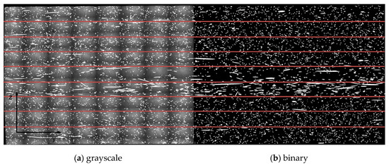
Figure 12.
Different states of image processing to determine the fiber orientation.
The fiber orientation distribution along the sample thickness (z-direction) of each individual sample is obtained from overall 15 grid points by the calculated cell averages. In Addition, two cross sections of each material and process setting were analyzed and averaged to eliminate measurement and processing deviations. For example, Figure 13a shows the fiber orientation results for two samples and the averaged curve.
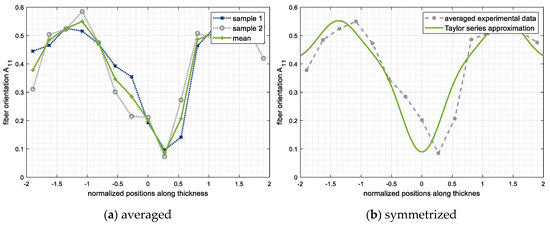
Figure 13.
Processing of the fiber orientation results for objective comparison (PP-LGF20 v30).
Even though two samples were averaged, an objective calibration of the fiber orientation model on the basis of only few measuring points is usually not reasonable. Furthermore, the experimentally determined fiber orientation shows a slightly off-center position of the core layer, which is caused by an uneven mold cooling as already observed in [101]. To obtain comparable results for experiment and simulation, the measuring points are symmetrized towards the center and smoothed by approximation. However, the characteristic properties of the curve progression regarding the fiber properties in the core and shear layer should be retained. For this purpose, the measuring points are represented by a fifth-order Taylor series approximation, as shown in Figure 13b for the orientation tensor entry . This method allows an objective comparison between simulation and experiment, independently of the number of measured data points. In addition, the curves are symmetrized without a significant change in their characteristic shape.
2.3. Process Simulation
The process simulation was performed with Moldex3D® of CoreTech System, Chupei City, Taiwan, which numerically solves the governing Equations (2)–(4). The calculated geometry is a complete model of the injection molded plate as shown in Figure 11a. The mesh was made by Rhinozeros 5 from Robert McNeel & Associates, Seattle, USA, and is shown in Figure 14a. The plates were meshed with a structured grid consisting of 21 hexahedral elements along the thickness of 4 mm, whereas tetrahedral elements were used for the runner system and sprue. A constant velocity according to the injection speed was set at the Inlet. The viscosities of the individual materials PP-LGF20, PP-LGF40, and PP-LGF60 were determined by means of a high-pressure capillary rheometer in the range of high shear rates, and a rotational rheometry for low shear rates. The experimental data was fitted by the Herschel–Bulkley viscosity model as shown in Figure 14b.
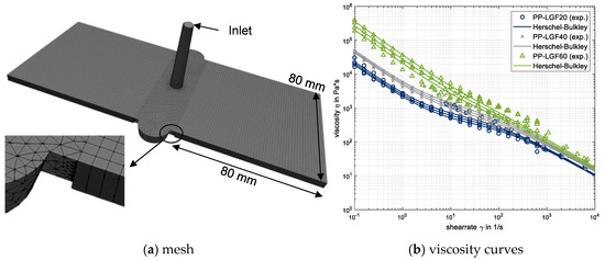
Figure 14.
Geometry and material setup of the simulation model.
The results of the viscosity determination show the expected rise of the viscosity with higher fiber content, especially for relatively low shear rates. The respective model parameters for the prediction of the fiber orientation model are determined by different iterative optimization methods described in the following sections, which compare the simulation results to the experimental measured data. The pvT-model for the thermodynamic state relations according to [115] was used to describe the density of the fluid as a function of temperature and pressure. All other necessary boundary conditions, such as injection speed as well as melt and mold temperatures, were defined according to the injection molding processing conditions described in Section 2.1.
In order to investigate the influence of the different versions of the iARD fiber orientation model as explained in Section 1.1.8 on the resulting fiber orientation distribution the following software versions of Moldex3D® with the different fiber orientation model versions
- basic iARD model in version R13,
- enhanced iARD model with shear rate dependency in version R16,
- and enhanced iARD model with shear rate dependency and fiber coupled viscosity in R17 were used.
Because fiber length is significantly reduced within the plastification unit, and this is not part of the simulation, the number averaged fiber length (see Table 1) was experimentally measured as described in [36] at the sprue and specified as a boundary condition in the respective process simulations. As expected, the results show that, with an increasing fiber content, the probability of fiber–fiber interaction increases significantly, and fiber breakage occur more frequently.

Table 1.
Experimentally determined number average fiber length at the sprue.
2.4. Adjustment of the Fiber Orientation Model within Process Simulation
2.4.1. Comparison of Simulation and Experimental Data
In order to objectively compare the predicted fiber orientation distribution along the thickness with the experimentally determined data, the least square error is calculated by Equation (21) at all positions of a sample according to Figure 11b.
To reduce the optimization problem, only the three orientation tensor components , , and were added as least square functions. Furthermore, the minimum square error functions can be weighted differently if the adaptation to a certain orientation direction takes priority.
2.4.2. Influence of the Fiber Orientation Model Parameters
Another considerable factor is the accurate calibration of the model parameters , , and , which can influence the core-layer thickness (mainly ) as well as the degree of orientation in the skin layers (mainly and ). In comparison of different fiber orientation model versions implemented in Moldex3D® as described in Section 2.3 the influence of the three parameters changes significantly. As shown in Figure 15a change of and within the basic iARD model mainly result in a different degree of orientation inside the skin layers, whereas α leads to a change in the core layer thickness. With more recent enhancements of the orientation model iARD with shear rate dependency in R16 and also with fiber coupled viscosity in R17, the parameter α shows hardly any change in the core layer thickness Figure 15b,c. This also leads to a very small transition zone between the core and skin layers.
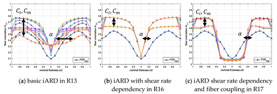
Figure 15.
Influence of fiber orientation model parameters on different software versions.
Even though the basic iARD fiber orientation model implemented in Moldex3D® version R13 is considerably older than the other versions, only this version allows to adjust the core layer thickness by means of the corresponding fiber orientation model parameters. According to this study, the basic iARD model has the most individual configuration parameters to represent the experimentally determined fiber orientation as accurately as possible.
2.5. Calibration of Fiber Orientation Model
Based on the calibration and optimization methods explained in Section 1.1.9 and Section 1.1.10, a detailed description of the methods used in this article is given below.
2.5.1. Direct Optimization
In order to directly optimize the results of the fiber orientation model iARD, the respective model parameters , Cm and have to be adjusted until the defined optimization objective is reached. However, the optimization algorithms require input variables as well as output variables, which can be described by the functions or directly adjusted. Therefore, a specific routine is needed, which changes the fiber orientation model parameters inside the simulation environment, starts the simulation run with the defined parameters, waits until the simulation is successfully calculated, reads out the defined results (i.e., fiber orientation tensor component along the thickness at a specified location of the part), and transfers these results as input parameters to the optimization algorithm, and compares the results with a defined optimization objective. Finally, depending on the optimization objective and the associated accuracy, the optimization procedure must be terminated or the routine must be restarted. In this work, the described optimization approach was implemented in a MATLAB® script, which directly accesses the input data of Moldex3D®, and thus creates new runs and triggers their calculation.
2.5.2. A New Calibration Method
In a new method, the fiber orientation calculation and its optimization were performed with a MATLAB® script according to the process scheme shown in Figure 16.

Figure 16.
Process scheme of the fiber orientation optimization tool.
To obtain the necessary flow field for the injection molding process, the results (velocity gradient tensor ) of a single initial injection molding simulation in Moldex3D® were exported and used in MATLAB® to calculate the corresponding fiber orientation model by means of Equations (5)–(15) (basic iARD model). Based on the initial calculation of the flow field, the whole parameter optimization of the fiber orientation model was carried out within a few minutes.
The main intention of this method was not the development a new optimization algorithm, but the removal of the time-consuming recalculation of the entire flow field for each optimization step (in contrast to the direct optimization described in Section 2.5.1). By using the flow field of an initial injection molding simulation, the computation is reduced to the calculation of the fiber orientation model.
The goal of the optimization was to minimize the objective function, consisting of the error sum of squares between simulative calculated and experimental determined fiber orientations at pre-defined positions. A gradient-based algorithm according to Section 1.1.10 was used for this purpose. This means that at the current point of the optimization, the first derivative for the direction of the optimization step and second derivatives for the length of the iteration step for each variable are used.
Because this case is a multi-parameter optimization, a system of Equations (22) is required to solve a variation step. This is as follows for the three parameters of the fiber orientation model.
In this form, only the main diagonals of the matrix are filled, which changes the optimization to a quasi-Newtonian method. In this form, fewer derivatives are needed to calculate the variation vector, which makes the calculation much more timesaving. Furthermore, the addition of scaling is also simplified. The Hessian matrix is positive definite, and thus the correct direction of the variation step is determined. Additionally, all three parameters are assigned to limits.
For this reason, an additional line search method is introduced to guarantee that these limits are observed. To prevent the optimization from getting stuck at these limits, a damping factor ∝D is introduced in Equation (23) in addition to the line search factor .
From all restrictions, the value is determined. Furthermore, a line search factor is used to prevent oscillation. For this purpose, it is verified whether the target function value increases contrary to the expectation during the optimization. In this case, the optimization step is shortened greatly with to allow only a small deterioration. For this purpose, the factor is specified if . Because the optimization problem can be dominated by the restrictions, the following is suggested for the damping factor:
- if is active
- without active constraint
This is to prevent the optimizer from getting stuck at the given variable boundaries. This problem is further improved by the introduction of scaling for the Hessian matrix (Equation (24)).
With the damping factor , the barrier is approached more slowly, and the other two parameters are weighted more heavily.
3. Results
In this Section, the influences of different material and process settings are evaluated. Based on the experimental data, the optimization results for the simulation are shown, and the two different optimization methods are compared.
3.1. Experimental Results
3.1.1. Fiber Orientation at Different Positions
The following Figure 17a shows the fiber orientation distribution along the plate thickness at three different positions (according to Figure 13, Pos. A, B, and C) along the flow path. In addition, the experimental results were smoothed and symmetrized according to Section 3.2 in order to be compared with the simulated results, Figure 17b.
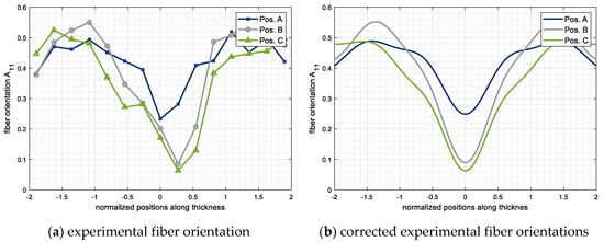
Figure 17.
Experimentally determined fiber orientations along the flow path for PP-LGF20 v30.
The analysis of the fiber orientation distribution along the flow path (position A–C) shows an increasing core layer, which also means that more fibers are oriented perpendicular to the flow direction. This also leads to enhancement of the mechanical properties in this direction, while the properties in the flow direction are diminished. However, the increase in shear layer thickness along the flow path has often been observed and is not a particular phenomenon of long fiber reinforced plastics.
3.1.2. Fiber Orientation of Different Materials and Process Conditions
In the following section, the influence of fiber concentration and injection speed is analyzed. In general, it can be observed (Figure 18) that all fiber concentrations and processing conditions of the injection-molded long glass fiber reinforced polypropylene lead to a low degree of fiber orientation in the shear layers, and a wide core layer with a high degree of orientation.
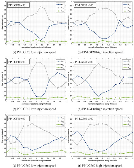
Figure 18.
Resulting fiber orientation along the thickness of different fiber concentrations (20, 40 and 60% mass fraction long glass fiber) and different injection speeds (low = 30 cm3/s, high = 100 cm3/s).
All the analyzed specimens show a higher degree of orientation perpendicular to the flow () than parallel to the flow direction () in the core layer region, whereas in the shear layers, the degree of orientation is nearly the same in both directions (parallel and perpendicular to the flow ). This effect changes only imperceptibly, even with a variation in fiber concentration and injection speed. In contrast to short fiber reinforced plastics, the wide core layer with its high degree of fiber orientation in the long fiber reinforced material also leads to higher mechanical properties (e.g., stiffness, strengthm and impact resistance as shown in Figure 1) perpendicular to the flow. A unique detail of the analyzed parts can be observed in the shifted core layers, which are not completely centered. This effect is caused by a different cooling performance (comparable to [101]) of the mold halves and has no influence on the interpretation of the results.
The analysis of the three different fiber concentrations (fiber mass fractions 20%, 40%, and 60%) of the long glass fiber reinforced polypropylene also show that an increase in fiber concentration results in a more distinct core layer Figure 18a,c,e. This means that a more concentrated suspension leads to an increased number of fibers that are oriented perpendicular to the flow direction . The same effect can also be seen in the variation of the injection speed. With increasing flow velocity, a wider core layer can be observed for all analyzed fiber concentrations.
In order to compare the skin core layer ratio systematically, two different methods were developed and used in this study. As a first method, the entry of the fiber orientation tensor is approximated by a function, and the transition from skin to core layer (green line) is determined by the mean value of the two inflection points of its derivative as shown in Figure 19a. The determined threshold lines are also depicted in the grinded pattern of the cross section as shown in Figure 19b. Subsequently, the skin layer ratio can be calculated by the ratio of the associated thickness values. As a second method, the two intersections between the fiber orientation curves and are determined and their mean value is defined as the transition from skin to core.
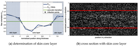
Figure 19.
Method to determine the skin core layer ratio of a reinforced material by objective criteria.
For the different materials and injection speeds the resulting skin core layer ratios showed only slight differences between the two described methods. Therefore, only the results of the intersection method of and were chosen and shown in Table 2.

Table 2.
Skin core layer ratio for different fiber concentrations and injection speeds of PP-LGF.
The results for the calculated skin-to-core layer ratios show an increase in the core-layer thickness with increasing fiber content. Thus, the previously recognized tendency of increase in core layer thickness can be proven objectively. The effect can be seen in general for low as well as for high injection speeds, except the outlying value for a very thin core layer thickness with 36% for PP-LGF40 at a low injection speed. No reason has been found to explain this effect.
3.2. Results of the Parameter Optimization
As shown in Figure 15, the resulting fiber orientation distribution varies very strongly, depending on the chosen fiber orientation model parameters. Figure 20 shows the results of direct parameter optimization, as explained in Section 2.5.1, by coupling MATLAB® and Moldex3D® with different fiber orientation models, (a) basic iARD and (b) iARD with shear rate dependency.
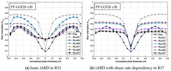
Figure 20.
Results of the direct parameter optimization by coupling MATLAB® and Moldex3D®.
To prove the functionality of the optimization routine, deviant values were chosen as initial parameters for the corresponding fiber orientation model (Run 1), which did not match the experiments. The experimentally determined fiber orientation is depicted as blue line with triangular markers. For a clearer presentation of the optimization progress, only some selected optimization steps are shown. However, the run numbers still correspond to the respective iteration step. The results obviously show a better agreement to the experiment with increasing iterations. In the skin layer, the optimization result of the basic iARD model shows very good accordance with the experimental data, whereas in the core layer, the simulation result does not represent the low degree of orientation determined by the experiment. However, this cannot be further improved by optimizing the model parameters, as there is no parameter set that can represent the entire orientation distribution from the experiment. This means that the best possible parameter set was found after 37 optimization steps for the basic iARD fiber orientation model.
For the optimization of the iARD model with shear rate dependency in version R17, the adjustment of the parameters has only a very one-dimensional influence on the change of the fiber orientation. Because the change from core to shear layer is very abrupt, no real transition zone is formed. Therefore, the degree of orientation in the skin layers can only be adjusted by varying the parameters and . All the other areas remain largely constant despite the parameter variation.
3.3. Influence of Parameters and Viscosity
In addition to the model parameters, the defined shear rate-dependent viscosity also has a significant influence on the resulting velocity profile as already explained in Section 1.1.2 as well as the results of the fiber orientation model. For this reason, the parameters of the defined viscosity model (Herschel–Bulkley) were varied and the influence on the fiber orientation distribution was investigated. Figure 21 shows the analyzed viscosity curves, which are moved slightly towards higher and lower viscosities (deviating from experimental data).
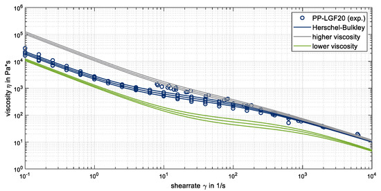
Figure 21.
Shear rate and temperature dependent viscosity and analyzed viscosity curves.
In Figure 22 the influence of the viscosity on the resulting fiber orientation distribution is investigated for different fiber orientation model versions and parameters (comparable to Figure 15). On the left side of Figure 22a,c,e, the fiber orientation was calculated with the experimentally determined viscosity for PP-LGF20 (blue curve in Figure 21), and on the right side of the Figure 22b,d,f, a higher viscosity, especially in the area of low shear rates (grey curve in Figure 21), is used. In the first row (a, b) the basic iARD model in Moldex3D® version R13, and in the second row (c, d) the iARD model with shear rate dependency in version R16, and the last row (e, f) the iARD model with shear rate dependency and fiber coupling in version R17 is used. For the comparison of the three fiber orientation model versions, the same variation of fiber orientation model parameters was used. The parameter was varied in the range of 0–0.99 for high and also low and values.
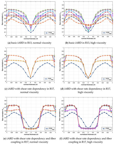
Figure 22.
Influence of the viscosity for different fiber orientation model versions for PP-LGF20v30.
First of all, all results show a change of the fiber orientation distribution within the core layer due to the change in viscosity. However, the fiber orientation distribution in the shear layers remains almost unchanged for all settings (viscosity models, fiber orientation models and parameters) due to the same viscosity in the range of high shear rates (blue and grey curve in Figure 21). The viscosity change mainly only affects the thickness of the core layer. The core layer is widened with a higher viscosity curve, which corresponds more closely to the experimental determined fiber orientation distribution. However, even if the adjustment of the viscosity curve improves the thickness of the core layer, a deviation between the predicted and measured fiber orientation still remains for all analyzed fiber orientation models, as well as for the viscosity models and their respective parameters.
3.4. Validation and Results of the New Calibration Approach
In order to ensure the correct implementation of the new optimization routine, a test case was chosen from literature [87]. Thus, the different parts of the implemented orientation model were tested for performance and verified by reference values [87]. The investigated test case is a simple shear flow within a single element. Two different versions of the fiber orientation models explained in Section 1.1.8, the basic iARD model (Equation (9)) and the iARD-RPR model (Equation (12)), were tested. The parameters of the fiber orientation model are chosen to make the iARD model ( and ) correspond to the standard model of Folgar-Tucker (FT) [86]. In Figure 23 the reference values are shown as points and the calculated fiber orientation as lines.
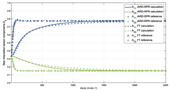
Figure 23.
Validation of the implemented fiber orientation calculation within the calibration tool.
The results of the fiber orientation calculation with the new calibration tool in Figure 23 show quite good agreement with the results from literature. Thus, a correct implementation of the fiber orientation model is assumed. A further validation can be obtained by comparing the calculation of the fiber orientation by Moldex3D® with the fiber orientation calculated by the new calibration tool in MATLAB® on the basis of the same flow field exported from Moldex3D®. The results of the calculated fiber orientation distribution are almost identical, as shown in Figure 24a.
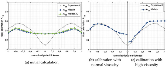
Figure 24.
Calculation and calibration results of the fiber orientation calibration tool.
Based on this initial calculation, a parameter optimization was performed with the calibration tool in MATLAB®. The calibration results of the parameter optimization are shown in Figure 24b for the experimentally measured viscosity, and in (c) for the increased viscosity according to the gray curve in Figure 21. Even if the fiber orientation model does not represent the entire orientation distribution, the adjusted viscosity curve (high viscosity) leads to a significant improvement in the resulting fiber orientation distribution in the core layer.
Compared with direct optimization by Moldex3D® (Section 2.5.1), the new calibration approach (Section 2.5.2) fully implemented in MATLAB® is significantly faster, as the entire calculation is based on only one initial calculation of the flow field without any necessary recalculation. The following Figure 25 clearly demonstrates that a significant amount (approximately factor 15) of the required calculation time can be saved by the new approach. Because the calculation of the fiber orientation is performed as an independent post-processing step, the calculation of the flow field is independent of the fiber orientation calculation and remains the same for each optimization step.
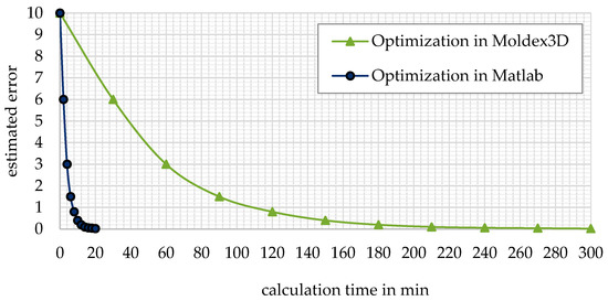
Figure 25.
Comparison of calculation time of direct optimization method and the new optimization approach implemented in the fiber orientation optimization tool.
4. Conclusions and Outlook
A novel method for the objective comparison of experimentally determined and by process simulation predicted fiber orientation was developed. As a first step, a new standardized method for the objective comparison of experimentally determined and simulation predicted fiber orientation based on the error deviation was defined. Furthermore, a corresponding validation of the method showed that the fiber orientation model has successfully been implemented in the novel calibration tool, and that the developed problem-specific optimization algorithm can adjust the model parameters simultaneously in order to minimize the objective function.
After only a few iteration loops and within a few minutes, the automated method shows an optimized fiber orientation distribution for long fiber reinforced materials based on the calculated flow field. Thus, the model parameters for the fiber orientation model are determined in the most accurate way and can be used for further predictions. This also allows for calculating the structural mechanics of fiber reinforced parts with high prediction accuracy. These results clearly confirm the scientific hypotheses stated at the beginning of this study.
The investigation also showed that there is further optimization potential which should be investigated and considered in the future. The parameter optimization is currently only implemented for the fiber orientation model, but can easily be extended to the prediction of fiber length distribution and fiber concentration. Further development of this method also allows a transfer of the calculated properties to structural mechanics with high quality predictions.
Author Contributions
Conceptualization, F.W. and P.R.; methodology, F.W. and P.R.; software, F.W. and P.R.; validation, F.W. and P.R.; formal analysis, F.W. and P.R.; investigation, F.W. and P.R.; resources, F.W. and P.R.; data curation, F.W. and P.R.; writing—original draft preparation, F.W. and P.R.; writing—review and editing, F.W., P.R. and C.B.; visualization, F.W. and P.R.; supervision, C.B.; project administration, F.W.; funding acquisition, C.B. All authors have read and agreed to the published version of the manuscript.
Funding
This research was funded by the German Federal Ministry of Economics and Energy (BMWi) within the Central Innovation Program for SMEs (ZIM). Grant number [ZF4041122BL7].
Conflicts of Interest
The authors declare no conflict of interest.
References
- Tseng, H.-C.; Chang, R.-Y.; Hsu, C.-H. Numerical prediction of fiber orientation and mechanical performance for short/long glass and carbon fiber-reinforced composites. Compos. Sci. Technol. 2017, 144, 51–56. [Google Scholar] [CrossRef]
- Mu, Y.; Chen, A.; Zhao, G.; Cui, Y.; Feng, J.; Ren, F. Prediction for the mechanical property of short fiber-reinforced polymer composites through process modeling method. J. Thermoplast. Compos. Mater. 2019, 32, 1525–1546. [Google Scholar] [CrossRef]
- Fu, S.-Y.; Lauke, B.; Mai, Y.W. Science and engineering of short fibre reinforced polymers composites. In Woodhead Publishing in Materials; Woodhead Publishing: Cambridge, UK; Boca Raton, FL, USA, 2009. [Google Scholar]
- Folkes, M.J. Short fibre reinforced thermoplastics. In Polymer Engineering Research Studies Series; Research Studies Press: Chichester, UK, 1985; Volume 1. [Google Scholar]
- Goris, S.; Osswald, T.A. Process-induced fiber matrix separation in long fiber-reinforced thermoplastics. Compos. Part A Appl. Sci. Manuf. 2018, 105, 321–333. [Google Scholar] [CrossRef]
- Tseng, H.-C.; Chang, R.-Y.; Hsu, C.-H. Improved fiber orientation predictions for injection molded fiber composites. Compos. Part A Appl. Sci. Manuf. 2017, 99, 65–75. [Google Scholar] [CrossRef]
- Willems, F.; Bonten, C. The use of micromechanical models to predict fiber reinforced plastics. In Proceedings of the Europe/Africa Conference Dresden 2017—Polymer Processing Society PPS, Dresden, Germany, 27–29 June 2017. [Google Scholar] [CrossRef]
- Nguyen, B.N.; Bapanapalli, S.K.; Holbery, J.D.; Smith, M.T.; Kunc, V.; Frame, B.J.; Phelps, J.H.; Tucker, C.L. Fiber Length and Orientation in Long-Fiber Injection-Molded Thermoplastics—Part I: Modeling of Microstructure and Elastic Properties. J. Compos. Mater. 2008, 42, 1003–1029. [Google Scholar] [CrossRef]
- Tseng, H.-C.; Goto, M.; Chang, R.-Y.; Hsu, C.-H. Accurate predictions of fiber orientation and mechanical properties in long-fiber-reinforced composite with experimental validation. Polym. Compos. 2018, 39, 3434–3445. [Google Scholar] [CrossRef]
- Willems, F.; Bonten, C. Prediction of Fiber-Reinforced Plastics Considering Local Fiber Length and Orientation. W05-495. In Society of Plastics Engineers, (SPE), Proceedings of the SPE ANTEC 2018, Orlando, FL, USA, 7–10 May 2018; Curran Associates, Inc.: Red Hook, NY, USA, 2018; pp. 2649–2656. [Google Scholar]
- Garesci, F.; Fliegener, S. Young’s modulus prediction of long fiber reinforced thermoplastics. Compos. Sci. Technol. 2013, 85, 142–147. [Google Scholar] [CrossRef]
- van Haag, J.; Hopmann, C. Simulate “Longer”. A New Calculation Model Allows the Prediction of Strength of Long Fiber-Reinforced Thermoplastics by means of Integrative Simulation. Kunstst. Int. 2016, 2, 42–45. [Google Scholar]
- Kardos, J.L. Critical issues in achieving desirable mechanical properties for short fiber composites. Pure Appl. Chem. 1985, 57, 1651–1657. [Google Scholar] [CrossRef]
- Akay, M.; Barkley, D. Fibre orientation and mechanical behaviour in reinforced thermoplastic injection mouldings. J. Mater. Sci. 1991, 26, 2731–2742. [Google Scholar] [CrossRef]
- Mortazavian, S.; Fatemi, A. Effects of fiber orientation and anisotropy on tensile strength and elastic modulus of short fiber reinforced polymer composites. Compos. Part B Eng. 2015, 72, 116–129. [Google Scholar] [CrossRef]
- Osswald, T.A. Understanding polymer processing. In Processes and Governing Equations, 2nd ed.; Hanser Publishers: Cincinnati, OH, USA; Munich, Germany, 2017. [Google Scholar]
- Lees, J.K. A study of the tensile modulus of short fiber reinforced plastics. Polym. Eng. Sci. 1968, 8, 186–194. [Google Scholar] [CrossRef]
- Lees, J.K. A study of the tensile strength of short fiber reinforced plastics. Polym. Eng. Sci. 1968, 8, 195–201. [Google Scholar] [CrossRef]
- De Monte, M.; Moosbrugger, E.; Quaresimin, M. Influence of temperature and thickness on the off-axis behaviour of short glass fibre reinforced polyamide 6.6—Quasi-static loading. Compos. Part A Appl. Sci. Manuf. 2010, 41, 859–871. [Google Scholar] [CrossRef]
- Fu, S.-Y.; Lauke, B. Effects of fiber length and fiber orientation distributions on the tensile strength of short-fiber-reinforced polymers. Compos. Sci. Technol. 1996, 56, 1179–1190. [Google Scholar] [CrossRef]
- Fu, S.-Y.; Lauke, B. The elastic modulus of misaligned short-fiber-reinforced polymers. Compos. Sci. Technol. 1998, 58, 389–400. [Google Scholar] [CrossRef]
- Lauke, B.; Fu, S.-Y. Strength anisotropy of misaligned short-fibre-reinforced polymers. Compos. Sci. Technol. 1999, 59, 699–708. [Google Scholar] [CrossRef]
- Thomason, J.L.; Vlug, M.A. Influence of fibre length and concentration on the properties of glass fibre-reinforced polypropylene: 1. Tensile and flexural modulus. Compos. Part A Appl. Sci. Manuf. 1996, 27, 477–484. [Google Scholar] [CrossRef]
- Thomason, J.L. Structure–property relationships in glass reinforced polyamide, part 2: The effects of average fiber diameter and diameter distribution. Polym. Compos. 2007, 28, 331–343. [Google Scholar] [CrossRef] [Green Version]
- Thomason, J.L.; Vlug, M.A. Influence of fibre length and concentration on the properties of glass fibre-reinforced polypropylene: 4. Impact properties. Compos. Part A Appl. Sci. Manuf. 1997, 28, 277–288. [Google Scholar] [CrossRef]
- Thomason, J.L. The influence of fibre length and concentration on the properties of glass fibre reinforced polypropylene: 5. Injection moulded long and short fibre PP. Compos. Part A Appl. Sci. Manuf. 2002, 33, 1641–1652. [Google Scholar] [CrossRef]
- Toll, S.; Aronsson, C.-G. Notched strength of long- and short-fibre reinforced polyamide. Compos. Sci. Technol. 1992, 45, 43–54. [Google Scholar] [CrossRef]
- Vu-Khanh, T.; Denault, J. Toughness of Reinforced Ductile Thermoplastics. J. Compos. Mater. 1992, 26, 2262–2277. [Google Scholar] [CrossRef]
- Thomason, J.L. The influence of fibre length and concentration on the properties of glass fibre reinforced polypropylene: 7. Interface strength and fibre strain in injection moulded long fibre PP at high fibre content. Compos. Part A Appl. Sci. Manuf. 2007, 38, 210–216. [Google Scholar] [CrossRef] [Green Version]
- Kumar, K.S.; Bhatnagar, N.; Ghosh, A.K. Development of Long Glass Fiber Reinforced Polypropylene Composites: Mechanical and Morphological Characteristics. J. Reinf. Plast. Compos. 2007, 26, 239–249. [Google Scholar] [CrossRef]
- Gupta, M.; Wang, K.K. Fiber orientation and mechanical properties of short-fiber-reinforced injection-molded composites: Simulated and experimental results. Polym. Compos. 1993, 14, 367–382. [Google Scholar] [CrossRef]
- Bonten, C. Plastics Technology. In Introduction and Fundamentals; Carl Hanser Verlag GmbH & Co. KG: München, Germany, 2019. [Google Scholar]
- Barbosa, S.E.; Kenny, J.M. Analysis of the Relationship between Processing Conditions-Fiber Orientation-Final Properties in Short Fiber Reinforced Polypropylene. J. Reinf. Plast. Compos. 1999, 18, 413–420. [Google Scholar] [CrossRef]
- Singh, P.; Kamal, M.R. The effect of processing variables on microstructure of injection molded short fiber reinforced polypropylene composites. Polym. Compos. 1989, 10, 344–351. [Google Scholar] [CrossRef]
- Sharma, B.N.; Naragani, D.; Nguyen, B.N.; Tucker, C.L.; Sangid, M.D. Uncertainty quantification of fiber orientation distribution measurements for long-fiber-reinforced thermoplastic composites. J. Compos. Mater. 2018, 52, 1781–1797. [Google Scholar] [CrossRef]
- Willems, F.; Bonten, C. Influence of processing on the fiber length degradation in fiber reinforced plastic parts. In Proceedings of the Regional Conference Graz 2015—Polymer Processing Society PPS: Conference Papers, Graz, Austria, 21–25 September 2015; p. 20003. [Google Scholar] [CrossRef] [Green Version]
- Gandhi, U.N.; Goris, S.; Osswald, T.A.; Song, Y.-Y. Discontinuous fiber-reinforced composites. In Fundamentals and Applications; Hanser Publishers: Munich, Germany; Cincinnati, OH, USA, 2020. [Google Scholar]
- Hegler, R.P. Faserorientierung beim Verarbeiten kurzfaserverstärkter Thermoplaste. Kunststoffe 1984, 74, 271–277. [Google Scholar]
- Bailey, R.; Rzepka, B. Fibre Orientation Mechanisms for Injection Molding of Long Fibre Composites. Int. Polym. Process. 1991, 6, 35–41. [Google Scholar] [CrossRef]
- Bay, R.S.; Tucker, C.L. Fiber orientation in simple injection moldings. Part II: Experimental results. Polym. Compos. 1992, 13, 332–341. [Google Scholar] [CrossRef]
- Folkes, M.J.; Russell, D.A.M. Orientation effects during the flow of short-fibre reinforced thermoplastics. Polymer 1980, 21, 1252–1258. [Google Scholar] [CrossRef]
- Karger-Kocsis, J. Microstructure and Fracture Mechanical Performance of Short-Fibre Reinforced Thermoplastics. In Application of Fracture Mechanics to Composite Materials; Composite Materials Series; Elsevier: Amsterdam, The Netherlands, 1989; Volume 6, pp. 189–247. [Google Scholar]
- Toll, S.; Andersson, P.-O. Microstructure of long- and short-fiber reinforced injection molded polyamide. Polym. Compos. 1993, 14, 116–125. [Google Scholar] [CrossRef]
- Spahr, D.E.; Friedrich, K.; Schultz, J.M.; Bailey, R.S. Microstructure and fracture behaviour of short and long fibre-reinforced polypropylene composites. J. Mater. Sci. 1990, 25, 4427–4439. [Google Scholar] [CrossRef]
- Bright, P.F.; Crowson, R.J.; Folkes, M.J. A study of the effect of injection speed on fibre orientation in simple mouldings of short glass fibre-filled polypropylene. J. Mater. Sci. 1978, 13, 2497–2506. [Google Scholar] [CrossRef]
- Bailey, R.; Kraft, H. A Study of Fibre Attrition in the Processing of Long Fibre Reinforced Thermoplastics. Int. Polym. Process. 1987, 2, 94–101. [Google Scholar] [CrossRef]
- Karger-Kocsis, J.; Friedrich, K. Fracture behavior of injection-molded short and long glass fiber—Polyamide 6.6 composites. Compos. Sci. Technol. 1988, 32, 293–325. [Google Scholar] [CrossRef]
- O’Regan, D.; Akay, M. The distribution of fibre lengths in injection moulded polyamide composite components. J. Mater. Process. Technol. 1996, 56, 282–291. [Google Scholar] [CrossRef]
- Mondy, L.A.; Brenner, H.; Altobelli, S.A.; Abbott, J.R.; Graham, A.L. Shear-induced particle migration in suspensions of rods. J. Rheol. 1994, 38, 444–452. [Google Scholar] [CrossRef]
- Lafranche, E.; Krawczak, P.; Ciolczyk, J.P.; Maugey, J. Injection moulding of long glass fibre reinforced polyamide 6-6: Guidelines to improve flexural properties. Express Polym. Lett. 2007, 1, 456–466. [Google Scholar] [CrossRef]
- Gruber, G.; Wartzack, S. Evaluierung der orientierungsbezogenen Leichtbaugüte. Lightweight Des. 2013, 6, 18–23. [Google Scholar] [CrossRef]
- Kenig, S. Fiber orientation development in molding of polymer composites. Polym. Compos. 1986, 7, 50–55. [Google Scholar] [CrossRef]
- Katti, S.S.; Schultz, M. The microstructure of injection-molded semicrystalline polymers: A review. Polym. Eng. Sci. 1982, 22, 1001–1017. [Google Scholar] [CrossRef]
- Friedrich, K. Microstructural efficiency and fracture toughness of short fiber/thermoplastic matrix composites. Compos. Sci. Technol. 1985, 22, 43–74. [Google Scholar] [CrossRef]
- Jiang, J.; Wang, S.; Hou, J.; Zhang, K.; Wang, X.; Li, Q.; Liu, G. Effect of injection velocity on the structure and mechanical properties of micro injection molded polycarbonate/poly(ethylene terephthalate) blends. Mater. Des. 2018, 141, 132–141. [Google Scholar] [CrossRef]
- Osswald, T.A.; Rudolph, N. Polymer rheology. In Fundamentals and Applications; Hanser Publications: Cincinnati, OH, USA, 2014. [Google Scholar]
- Guell, D.C.; Papathanasiou, T.D. Flow-Induced Alignment in Composite Materials; Woodhead: Cambridge, UK, 1997. [Google Scholar]
- Stommel, M.; Stojek, M.; Korte, W. FEM Zur Berechnung von Kunststoff- und Elastomerbauteilen, 2nd ed.; Hanser: München, Germany, 2018. [Google Scholar]
- Sigmasoft: 3D Moulding Simulation—The ‘Whole Process’ Approach. Met. Powder Rep. 2013, 68, 30–32. Available online: https://www.sciencedirect.com/science/article/abs/pii/S0026065713700948?via%3Dihub (accessed on 29 October 2020). [CrossRef]
- Advani, S.G.; Tucker, C.L. The Use of Tensors to Describe and Predict Fiber Orientation in Short Fiber Composites. J. Rheol. 1987, 31, 751–784. [Google Scholar] [CrossRef]
- Predak, S.; Solodov, I.Y.; Busse, G.; Bister, V.H.; Vöhringer, M.C.; Haberstroh, E.; Ehbing, H. Faserorientierungsmessung an kurzfaserverstärkten PUR-RIM-Bauteilen: Kombination zerstörungsfreier Prüfmethoden zur Optimierung von Simulation und Herstellungsprozess, (Fiber Orientation Measurement on Short Fiber Reinforced PUR-RIM Components: Combination of Nondestructive Testing Methods for Optimization of Simulation and Production Process). TM Tech. Mess. 2006, 73, 3. [Google Scholar] [CrossRef]
- Predak, S. Mikrowellen-Orientierungsmessungen zur Zerstörungsfreien Charakterisierung Kurzfaserverstärkter Kunststoffe; Publication Server of the University of Stuttgart: Stuttgart, Germany, 2007. [Google Scholar]
- Toll, S.; Andersson, P.-O. Microstructural characterization of injection moulded composites using image analysis. Composites 1991, 22, 298–306. [Google Scholar] [CrossRef]
- Hine, P.J.; Davidson, N.; Duckett, R.A.; Ward, I.M. Measuring the fibre orientation and modelling the elastic properties of injection-moulded long-glass-fibre-reinforced nylon. Compos. Sci. Technol. 1995, 53, 125–131. [Google Scholar] [CrossRef]
- McGee, S.H.; McCullough, R.L. An Optical Technique for Measuring Fiber Orientation in Short Fiber Composites. In The Role of the Polymeric Matrix in the Processing and Structural Properties Composite Materials; Seferis, J.C., Nicolais, L., Eds.; Springer: Boston, MA, USA, 1983; Volume 64, pp. 425–436. [Google Scholar]
- Mlekusch, B. Fibre orientation in short-fibre-reinforced thermoplastics II. Quantitative measurements by image analysis. Compos. Sci. Technol. 1999, 59, 547–560. [Google Scholar] [CrossRef]
- Fakirov, S.; Fakirova, C. Direct determination of the orientation of short glass fibers in an injection-molded poly(ethylene terephthalate) system. Polym. Compos. 1985, 6, 41–46. [Google Scholar] [CrossRef]
- Eberhardt, C.; Clarke, A. Fibre-orientation measurements in short-glass-fibre composites. Part I: Automated, high-angular-resolution measurement by confocal microscopy. Compos. Sci. Technol. 2001, 61, 1389–1400. [Google Scholar] [CrossRef]
- Vélez-García, G.M.; Wapperom, P.; Baird, D.G.; Aning, A.O.; Kunc, V. Unambiguous orientation in short fiber composites over small sampling area in a center-gated disk. Compos. Part A Appl. Sci. Manuf. 2012, 43, 104–113. [Google Scholar] [CrossRef]
- Willems, F.; Beerlink, A.; Metayer, J.-F.; Kreutzbruck, M.; Bonten, C. Bestimmung der Faserorientierung langglasfaserverstärkter Thermoplaste mittels Bildoptischer Analyse und Computertomografie; Deutsche Gesellschaft für Zerstörungsfreie Prüfung e.V, Ed.; DGZfP Jahrestagung: Leipzig, Germany, 7–9 May 2018.
- Kim, E.G.; Park, J.K.; Jo, S.H. A study on fiber orientation during the injection molding of fiber-reinforced polymeric composites. J. Mater. Process. Technol. 2001, 111, 225–232. [Google Scholar] [CrossRef]
- Darlington, M.W.; McGinley, P.L.; Smith, G.R. Structure and anisotropy of stiffness in glass fibre-reinforced thermoplastics. J. Mater. Sci. 1976, 11, 877–886. [Google Scholar] [CrossRef]
- Grote, F. Schaumstoffe mit CT charakterisieren. Kunstst. Plast Eur. 1999, 89, 110–111. [Google Scholar]
- Bernasconi, A.; Cosmi, F.; Hine, P.J. Analysis of fibre orientation distribution in short fibre reinforced polymers: A comparison between optical and tomographic methods. Compos. Sci. Technol. 2012, 72, 2002–2008. [Google Scholar] [CrossRef]
- Shen, H.; Nutt, S.; Hull, D. Direct observation and measurement of fiber architecture in short fiber-polymer composite foam through micro-CT imaging. Compos. Sci. Technol. 2004, 64, 2113–2120. [Google Scholar] [CrossRef]
- Maisl, M.; Scherer, T.; Reiter, H.; Hirsekorn, S. Nondestructive Investigation of Fibre Reinforced Composites by X-Ray Computed Tomography. In Nondestructive Characterization of Materials; Höller, P., Hauk, V., Dobmann, G., Ruud, C.O., Green, R.E., Eds.; Springer: Berlin/Heidelberg, Germany, 1989; pp. 147–154. [Google Scholar]
- Robb, K.; Wirjadi, O.; Schladitz, K. Fiber Orientation Estimation from 3D Image Data: Practical Algorithms, Visualization, and Interpretation. In Proceedings of the 7th International Conference on Hybrid Intelligent Systems, (HIS 2007), Kaiserslautern, Germany, 17–19 September 2007; pp. 320–325. [Google Scholar] [CrossRef]
- Sun, X.; Lasecki, J.; Zeng, D.; Gan, Y.; Su, X.; Tao, J. Measurement and quantitative analysis of fiber orientation distribution in long fiber reinforced part by injection molding. Polym. Test. 2015, 42, 168–174. [Google Scholar] [CrossRef]
- Fischer, G.; Eyerer, P. Measuring spatial orientation of short fiber reinforced thermoplastics by image analysis. Polym. Compos. 1988, 9, 297–304. [Google Scholar] [CrossRef]
- Kennedy, P.; Zheng, R. Flow Analysis of Injection Molds, 2nd ed.; Hanser Publishers: Munich, Germany; Cincinnati, OH, USA, 2013. [Google Scholar]
- Advani, S.G. (Ed.) Flow and rheology in polymer composites manufacturing. In Composite Materials Series, Vol. 10; Elsevier: Amsterdam, The Netherlands, 1994. [Google Scholar]
- Papanastasiou, T.C. Flows of Materials with Yield. J. Rheol. 1987, 31, 385–404. [Google Scholar] [CrossRef]
- Han, S.; Wang, K.K.; Hieber, C.A.; Cohen, C. Characterization of the rheological properties of a fast-curing epoxy-molding compound. J. Rheol. 1997, 41, 177–195. [Google Scholar] [CrossRef]
- Cross, M.M. Relation between viscoelasticity and shear-thinning behaviour in liquids. Rheol. Acta 1979, 18, 609–614. [Google Scholar] [CrossRef]
- Jeffery, G.B. The motion of ellipsoidal particles immersed in a viscous fluid. Proc. R. Soc. Lond. A 1922, 102, 161–179. [Google Scholar] [CrossRef] [Green Version]
- Phelps, J.H.; Tucker, C.L. An anisotropic rotary diffusion model for fiber orientation in short- and long-fiber thermoplastics. J. Non-Newton. Fluid Mech. 2009, 156, 165–176. [Google Scholar] [CrossRef]
- Tseng, H.-C.; Chang, R.-Y.; Hsu, C.-H. Method and computer readable media for determining orientation of fibers in a fluid. U.S. Patent 8,571,828, 29 October 2013. [Google Scholar]
- Tseng, H.-C.; Chang, R.-Y.; Hsu, C.-H. Phenomenological improvements to predictive models of fiber orientation in concentrated suspensions. J. Rheol. 2013, 57, 1597–1631. [Google Scholar] [CrossRef]
- Tseng, H.-C.; Chang, R.-Y.; Hsu, C.-H. An objective tensor to predict anisotropic fiber orientation in concentrated suspensions. J. Rheol. 2016, 60, 215–224. [Google Scholar] [CrossRef]
- Du Chung, H.; Kwon, T.H. Invariant-based optimal fitting closure approximation for the numerical prediction of flow-induced fiber orientation. J. Rheol. 2002, 46, 169–194. [Google Scholar] [CrossRef] [Green Version]
- Tseng, H.-C.; Chang, R.-Y.; Hsu, C.-H. The use of shear-rate-dependent parameters to improve fiber orientation predictions for injection molded fiber composites. Compos. Part A Appl. Sci. Manuf. 2018, 104, 81–88. [Google Scholar] [CrossRef]
- Tseng, H.-C.; Chang, R.-Y.; Hsu, C.-H. Comparison of recent fiber orientation models in injection molding simulation of fiber-reinforced composites. J. Thermoplast. Compos. Mater. 2020, 33, 35–52. [Google Scholar] [CrossRef]
- Willems, F.; Bonten, C. Structural prediction of injection molded long fiber reinforced plastics based on process induced fiber microstructure. In Proceedings of the International Conference on Composite Materials, 22nd, Melbourne, Australia, 11–16 August 2019; ICCM22. ICCM 22 2019. Engineers Australia, Ed.; Engineers Australia: Barton, Australia, 2019; pp. 4822–4831. [Google Scholar]
- Morak, M.; Tscharnuter, D.; Lucyshyn, T.; Hahn, W.; Göttlinger, M.; Kummer, M.; Steinberger, R.; Gross, T. Optimization of fiber prediction model coefficients in injection molding simulation based on micro computed tomography. Polym. Eng. Sci. 2019, 59, E152–E160. [Google Scholar] [CrossRef]
- Meyer, K.J.; Hofmann, J.T.; Baird, D.G. Prediction of short glass fiber orientation in the filling of an end-gated plaque. Compos. Part A Appl. Sci. Manuf. 2014, 62, 77–86. [Google Scholar] [CrossRef]
- Nguyen, B.N.; Jin, X.; Wang, J.; Phelps, J.; Tucker III, C.L.; Kunc, V.; Bapanapalli, S.K.; Smith, M.T. Implementation of New Process Models for Tailored Polymer Composite Structures into Processing Software Packages; Pacific Northwest National Lab. (PNNL): Richland, WA, USA, 2010. [Google Scholar]
- Foss, P.H.; Tseng, H.-C.; Snawerdt, J.; Chang, Y.-J.; Yang, W.-H.; Hsu, C.-H. Prediction of fiber orientation distribution in injection molded parts using Moldex3D simulation. Polym. Compos. 2014, 35, 671–680. [Google Scholar] [CrossRef]
- Phelps, J.H. Processing-Microstructure Models for Short- and Long-Fiber Thermoplastic Composites. Ph.D. Thesis, University of Illinois at Urbana-Champaign, Champaign, IL, USA. Available online: https://search.proquest.com/docview/304896821?accountid=14133 (accessed on 16 September 2017).
- Eberle, A.P.R.; Vélez-García, G.M.; Baird, D.G.; Wapperom, P. Fiber orientation kinetics of a concentrated short glass fiber suspension in startup of simple shear flow. J. Non-Newton. Fluid Mech. 2010, 165, 110–119. [Google Scholar] [CrossRef]
- Ortman, K.; Baird, D.; Wapperom, P.; Whittington, A. Using startup of steady shear flow in a sliding plate rheometer to determine material parameters for the purpose of predicting long fiber orientation. J. Rheol. 2012, 56, 955–981. [Google Scholar] [CrossRef] [Green Version]
- Bay, R.S. Fiber Orientation in Injection-Molded Composites: A Comparison of Theory and Experiment. Ph.D. Thesis, University of Illinois at Urbana-Champaign, Champaign, IL, USA, 1991. [Google Scholar]
- Phan-Thien, N.; Fan, X.-J.; Tanner, R.I.; Zheng, R. Folgar–Tucker constant for a fibre suspension in a Newtonian fluid. J. Non Newton. Fluid Mech. 2002, 103, 251–260. [Google Scholar] [CrossRef]
- Favaloro, A.J.; Tucker, C.L. Analysis of anisotropic rotary diffusion models for fiber orientation. Compos. Part A Appl. Sci. Manuf. 2019, 126, 105605. [Google Scholar] [CrossRef]
- Kugler, S.K.; Kech, A.; Cruz, C.; Osswald, T. Fiber Orientation Predictions—A Review of Existing Models. J. Compos. Sci. 2020, 4, 69. [Google Scholar] [CrossRef]
- Willems, F.; Bonten, C. Prediction of the Mechanical Properties of Long Fiber Reinforced Thermoplastics. In Proceedings of the PPS2019—PPS Europe-Africa Regional Conference, Pretoria, South Africa, 18–21 November 2019. [Google Scholar]
- Wonisch, A.; Wüst, A. More Precise Part Design. Accurate Simulation of Fiber Orientation of Glass Fiber-Reinforced Plastics. Kunstst. Int. 2014, 9, 80–83. [Google Scholar]
- Li, T.; Luyé, J.-F. Optimization of Fiber Orientation Model Parameters in the Presence of Flow-Fiber Coupling. J. Compos. Sci. 2018, 2, 73. [Google Scholar] [CrossRef] [Green Version]
- Kugler, S.K.; Lambert, G.M.; Cruz, C.; Kech, A.; Osswald, T.A.; Baird, D.G. Efficient parameter identification for macroscopic fiber orientation models with experimental data and a mechanistic fiber simulation. In Proceedings of the 35th International Conference of the Polymer Processing Society, (PPS-35), Cesme-Izmir, Turkey, 26–30 May 2019; AIP Publishing: Melville, NY, USA, 2020; p. 20050. [Google Scholar] [CrossRef]
- Reitinger, P.; Willems, F.; Bonten, C. Calibration of Models to Predict the Fiber Microstructure of LFRTs. In Proceedings of the PPS2019—PPS Europe-Africa 2019 Regional Conference, Pretoria, South Africa, 18–21 November 2019. [Google Scholar]
- Nocedal, J.; Wright, S. Numerical Optimization. Springer Series in Operations Research and Financial Engineering; Springer: New York, NY, USA, 2006. [Google Scholar]
- Poljak, B.T.; Poljak, B.T. Introduction to optimization. Translations Series in mathematics and engineering. In Optimization Software; Publications Division: New York, NY, USA, 1987. [Google Scholar]
- Feilmeier, M. Parameteroptimierung. In Hybridrechnen. International Series of Numerical Mathematics/Internationale Schriftenreihe zur Numerischen Mathematik/Série Internationale D’Analyse Numérique; Birkhäuser: Basel, Switzerland, 1974; Volume 2, pp. 243–259. [Google Scholar]
- Bertsekas, D.P. Projected Newton Methods for Optimization Problems with Simple Constraints. SIAM J. Control Optim. 1982, 20, 221–246. [Google Scholar] [CrossRef] [Green Version]
- Ning, H.; Lu, N.; Hassen, A.A.; Chawla, K.; Selim, M.; Pillay, S. A review of Long fibre thermoplastic, (LFT) composites. Int. Mater. Rev. 2020, 65, 164–188. [Google Scholar] [CrossRef]
- van Krevelen, D.W. Properties of Polymers: Their Correlation with Chemical Structure; Their Numerial Estimation and Prediction from Additive Group Contributions, 3rd ed.; Elsevier Science: Oxford, UK, 1997. [Google Scholar]
Publisher’s Note: MDPI stays neutral with regard to jurisdictional claims in published maps and institutional affiliations. |
© 2020 by the authors. Licensee MDPI, Basel, Switzerland. This article is an open access article distributed under the terms and conditions of the Creative Commons Attribution (CC BY) license (http://creativecommons.org/licenses/by/4.0/).