Article

An Efficient Method to Determine the Thermal Behavior of Composite Material with Loading High Thermal Conductivity Fillers

by
Chi-Cuong Tran
1 and
Quang-Khoi Nguyen
2,*
1
Department of Mechanical Engineering, National Taiwan University of Science and Technology, Taipei 10607, Taiwan
2
Department of Optics and Photonics, National Central University, Chungli 32001, Taiwan
*
Author to whom correspondence should be addressed.
J. Compos. Sci. 2022, 6(7), 214; https://doi.org/10.3390/jcs6070214
Submission received: 15 June 2022 / Revised: 4 July 2022 / Accepted: 14 July 2022 / Published: 20 July 2022
(This article belongs to the Special Issue Polymeric Composites Reinforced with Natural Fibers and Nanofillers)

Abstract

:
Improvement of the thermal conductivity of encapsulant material using doping filler is an important requirement for electronic device packaging. We proposed a simple method for determining the thermal characteristics of composite material that can help save time, increase research performance, and reduce the cost of buying testing equipment. Based on the theory of Fourier law, a general 3D model is simplified into a 2D model, which can then be applied to calculate the thermal conductivity of the tested sample. The temperature distribution inside the sample is simulated by the finite element method using MATLAB software; this is a simple and useful option for researchers who conduct studies on thermal conduction. In addition, an experimental setup is proposed to help determine the extent of thermal conductivity improvement in a sample with doping filler compared to a bare sample. This method is helpful for research on optoelectronics packaging, which relates to the enhancement of thermal conductivity composite material.

1. Introduction

High-power electronic devices always require an efficient way to manage heat, as generated heat is an avoidable problem for electronic devices during operation. For example, in the case of high-power phosphor converted white light emitting diodes (pcW-LEDs), due to the limitation of quantum efficiency and Stokes shift heat is always generated during operation. A portion of the input power is converted to useful power while the rest is converted to heat. That generated heat not only causes negative effects on the optical property of pcW-LEDs, such as color and wavelength shift, a shortened lifetime, and thermal degradation of output light [1,2,3], but also causes mechanical damage to the packaging structure [4]. It is reported that approximately 60% to 70% of input power is converted to heat [5,6]. Popular materials used to encapsulate pcW-LEDs are silicone resin and epoxy resin. Although the heat generated by electronics is substantial, the thermal conductivity of encapsulation material is 0.2 W/m.K [7]. This low thermal conductivity value limits the thermal management of electronic devices. It is necessary to reduce heat accumulation inside the packaging structure of the device. One method of heat management is increasing heat dissipation so that heat is transferred away from the heat source as fast as possible [8,9]. Effective heat conductive paths in the encapsulant material are crucial for the next generation of electronics packaging material.
It is well-known that polymer is widely used in electronic device packaging for many purposes, including protective layers, insulation, and to enhance light extraction. Heat dissipation ability can be increased if the thermal conductivity of encapsulant material is improved. It has been reported that the thermal conductivity of polymer can be enhanced by adding particle/material powder which has very high thermal conductivity [10,11,12,13,14,15,16,17,18]. Guo et al. reported that the thermal conductivity of TZnO/epoxy composites with 50 wt% filler reaches 4.38 W/m.K, an approximate 1816% enhancement compared to neat epoxy [10]. Wang et al. studied epoxy composite with carbon fibers (CFs) and alumina (Al2O3), and determined that the thermal conductivity of epoxy composite with 6.4 wt% CFs and 74 wt% Al2O3 hybrid filler reaches 3.84 W/m.K, which is a 2096% increase compared to neat epoxy [11]. Peng et al. reported that ZnO/epoxy nanocomposite film maintained high visible transparency (approximately 60–80%); the thermal conductivity of the composite is approximately 0.25–0.30 W/m.K with the content under 5 wt% of ZnO nanoparticles [12]. Shen et al. reported a facile approach to fabricate an epoxy composite incorporated with silicon carbide nanowires (SiC NWs). The thermal conductivity of epoxy/SiC NWs composite with 3.0 wt% filler reached 0.449 W/m.K, an approximate 106% enhancement compared to neat epoxy [13]. Ren et al. reported that thermal conductivity is significantly enhanced (~140%) in boron nitride nanoparticle (GBN)/epoxy composites containing only 5 wt% of GBN [14]. Gaska et al. studied the thermal conductivity of epoxy–matrix composites, and reported that epoxy filled with 31 vol.% of boron nitride–silica hybrid filler enhanced thermal conductivity by 114 % [15]. Yan et al. obtained a high value of thermal conductivity (1.73 W/m.K) for epoxy composites by constructing a dense thermal conductive network with a combination of alumina and carbon nanotubes [16]. Kang et al. used the 2D material, MXene (Ti3C2), as a reinforcement additive to optimize the thermal properties of polymers. The results showed that the thermal conductivity value (0.587 W/m.K) of epoxy composite with only 1.0 wt% Ti3C2 MXene fillers increased by 141.3% compared with that of neat epoxy [17]. Hu et al. discovered that a well-ordered boron nitride (BN) microstructure in the composites results in an elevated thermal conductivity up to 6.09 W/m.K at 50 wt% loadings [18]. In this type of research, it is important to test the changes in thermal conductivity of samples with doped fillers. There are several ways to determine materials’ thermal conductivity, including the steady-state technique, the nonsteady-state technique, the guarded hot plate, and laser flash diffusivity [19,20,21,22,23]. In terms of heat transfer engineering, in the steady-state the temperature of homogeneous material remains constant with time. In contrast, in the nonsteady-state the temperature of homogeneous material changes with time; this is also called a nonequilibrium or transient state. The key difference between thermal conductivity and diffusivity is that thermal conductivity refers to the ability of a material to conduct heat, whereas thermal diffusivity refers to the measurement of a material’s heat transfer rate from its hot ends to its cold ends. In general, a material that has considerable thermal conductivity will also have high thermal diffusivity, i.e., a high rate of heat transfer from high temperature ends to lower temperature ends. Thermal conductivity (K) can be calculated when the thermal diffusivity (α), specific heat capacity (Cp), and density ( ρ ) of a sample are known. Although most nonequivalent methods (or nonsteady-state techniques) are based on measuring thermal diffusivity, thermal conductivity (K) can be calculated from thermal diffusivity (α) through the relation: K = α ρ Cp, where Cp and ρ are specific heat capacity and density of the sample, respectively [24].
Researchers face expensive equipment costs when testing samples’ thermal conductivity; therefore, there is a demand for a simple, low cost, and effective way to determine a sample’s thermal conductivity. In addition to testing thermal conductivity, another important requirement is to know the temperature distribution inside the sample after thermal conductivity has been enhanced, as the thermal camera only detects temperature information on a sample‘s surface. Therefore, there is a demand for an additional method for internal thermal analysis to determine temperature behavior inside a sample. For that purpose, different simulation tools, such as COMSOL, QUICKFIELD, THESEUSFE, and MSC software, can be applied for thermal analysis purposes [25,26,27,28]. However, these types of expensive commercial software require sufficient programming ability. Interestingly, a familiar software, MATLAB, is also a useful tool to both solve the heat diffusion equation and intuitively present the temperature distribution [29,30,31]. Thus, if a thermal model is suitably built, the temperature distribution inside the sample can easily be obtained by applying the finite element method (FEM) in MATLAB.
In this paper, we proposed a method for determining the sample’s thermal conductivity using a thermoelectric cooler (TEC) and thermal camera. The temperature data obtained are used to calculate the enhancement of thermal conductivity by applying the theory of Fourier’s law. A simple model using MATLAB software simulates the internal temperature distribution corresponding to the thermal conductivity of the sample. The proposed method is helpful for heat management studies; it improves the thermal conduction of encapsulant material for electronic devices.

2. Theory of Calculation: The Improvement of Thermal Conductivity

Thermal conduction in one direction is illustrated in Figure 1.
For the one-dimension of thermal conduction, Fourier’s law can be written as
q = K d T d z
where q” is heat flux density (W/m2), which is the rate of heat transfer per unit area; K is thermal conductivity (W/m.K), which is a characteristic of the material; and dT is the temperature gradient along z direction [29]. The minus sign signifies that heat is transferred in the direction of decreasing temperature. Under steady-state conditions when the temperature is linear, the temperature gradient may be expressed as
d T d z = T 2 T 1 L
where L denotes the thickness of the sample; then, the heat flux density in Equation (1) becomes
q = K T 2 T 1 L
or
q = K T 1 T 2 L = K Δ T L
When the thermoelectric cooler (TEC) is powered, one surface becomes cool while the other surface becomes hot, based on the Peltier effect [32,33]. The TEC’s hot surface can be applied to heat samples; samples without and with doping high thermal conductivity (HTC) fillers are put on the same TEC’s hot surface. For the sample without doping HTC, apply the Equation (4), it obtains the equation
q = K 1 Δ T 1 L
Similar to the sample without doping HTC, the sample with doping HTC has
q = K 2 Δ T 2 L
As both samples are placed on the same TEC’s hot surface, heat flux transfers through samples without and with doping high thermal conductivity (HTC) fillers are the same. Thus, it obtains the relation
K 1 Δ T 1 L = K 2 Δ T 2 L
Or
K 2 K 1 = Δ T 1 Δ T 2
where K1 and K2 are thermal conductivity of plates without and with doping HTC material, respectively, and ΔT1 and ΔT2 are temperature differences between the bottom and top surfaces of plates without and with HTC, respectively.
Let n be the ratio of temperature difference between the samples’ bottom surface and top surface plates without doping HTC versus with doping HTC material; it thus has the following ratio
K 2 K 1 = Δ T 1 Δ T 2 = n Δ T 2 Δ T 2 = n
Finally, the thermal conductivity enhancement (TCE) of the sample with doping HTC compared to the sample without doping HTC can be determined as follows
TCE   ( % ) = K 2 K 1 K 1 × 100 = ( n 1 ) × 100
Figure 2 shows simulations of TCE for different values of n based on Equation (10). TCE is a function of the ratio of temperature difference (n). An increase in the sample’s thermo-conductivity will reduce the temperature difference between its two faces.

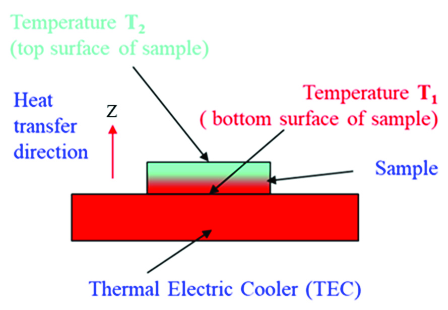
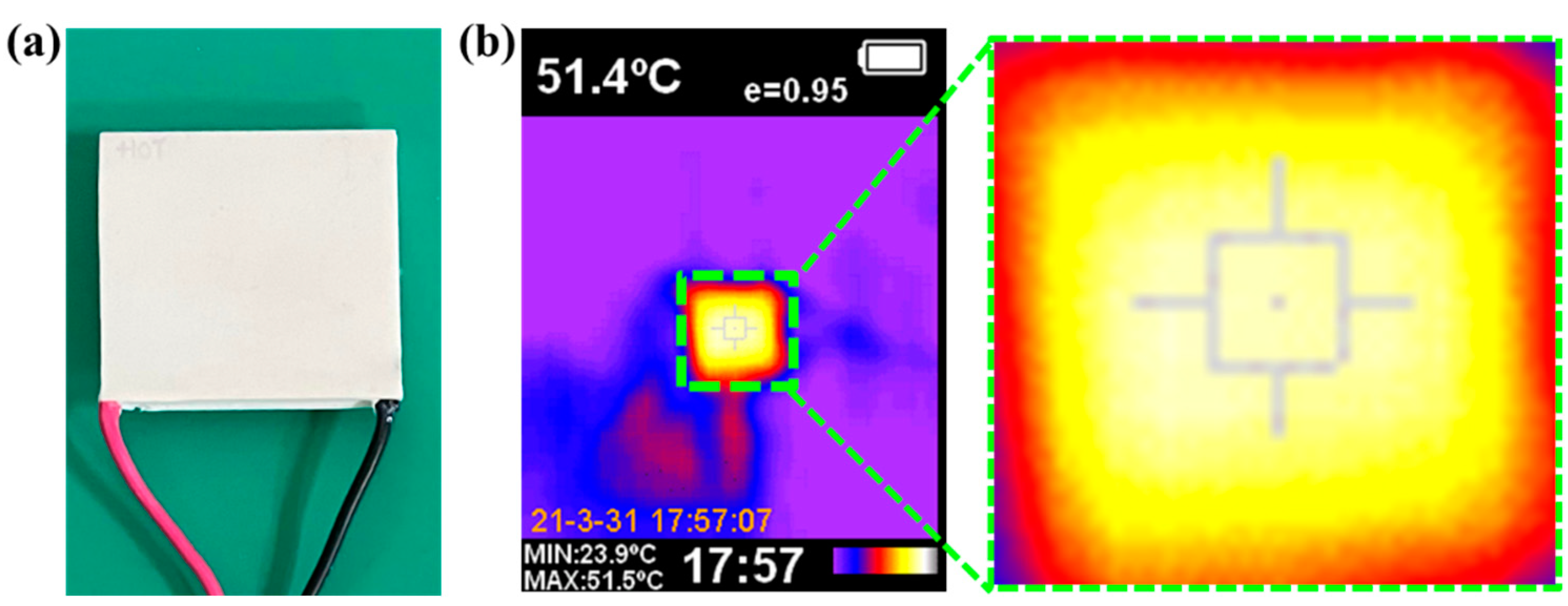
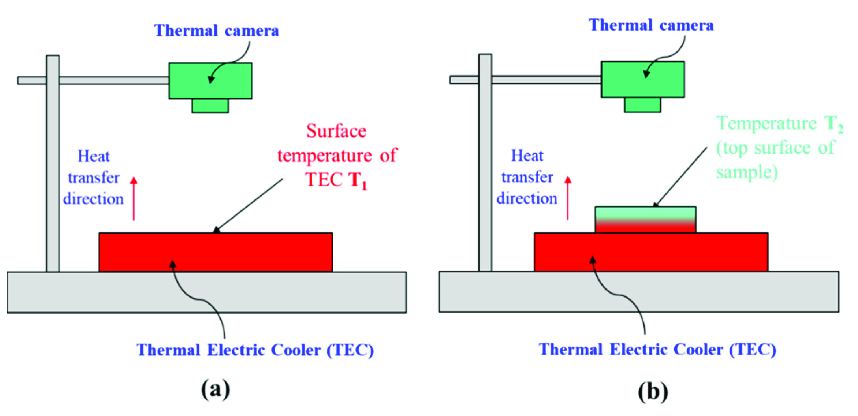
3. Method for Determining the Temperature Value of the Sample’s Two Faces in the Experiment

The equipment used are a TEC and a thermal camera. A TEC has the advantage of high uniform distribution on the hot surfaces, and is operated as shown in Figure 3. The test sample is put on the TEC’s hot surface. The temperature is measured using the thermal camera. If thermal contact with the sample’s bottom surface is sufficient, it can be assumed that the temperatures of the sample‘s bottom surface and the TEC’s hot surface are the same. The setup for measuring the temperature is shown in Figure 4. Figure 4a illustrates the thermal camera and the TEC device. Figure 4b illustrates the setup including the thermal camera, the TEC device, and the test sample. The setup in Figure 4a is used to determine the temperature of the TEC’s hot surface. Here, the temperature of the sample’s bottom surface is assumed to be the same as that of the TEC’s hot surface. The setup shown in Figure 4b is used to determine the temperature of the test sample’s top surface. The test sample is placed on the hot surface of the TEC. The sample is prepared as a thin cylindrical shape, with a thickness of 1 mm and a diameter of 16 mm, using the molding method.
Details of the experiment procedure’s setup as shown in Figure 4 are as follows. First, as depicted in Figure 4a, the temperature of the TEC’s hot surface is measured. In the thermal camera setting, select the parameter of thermal emissivity that corresponds to the material of the TEC‘s hot surface. When operating the TEC, wait for the thermal steady-state of the TEC device. Turn on the thermal camera to detect the temperature of the TEC’s hot surface. Second, for the experiment in Figure 4b, the process to determine the temperature of the sample’s top surface is as follows. The tested sample is placed on the top surface of the TEC. After waiting for the thermal steady-state, turn on the thermal camera and select the setting parameter of thermal emissivity that corresponds to the sample material. Shoot the thermal camera to obtain the temperature of the top surface of the sample.
Repeat the above process for additional bare samples and samples with different amounts of HTC material added to obtain their corresponding temperature differences between the bottom and top surfaces.
Finally, apply Equations (9) and (10) to calculate the changing of thermal conductivity or the TCE of the sample with added HTC compared to that of the bare sample.

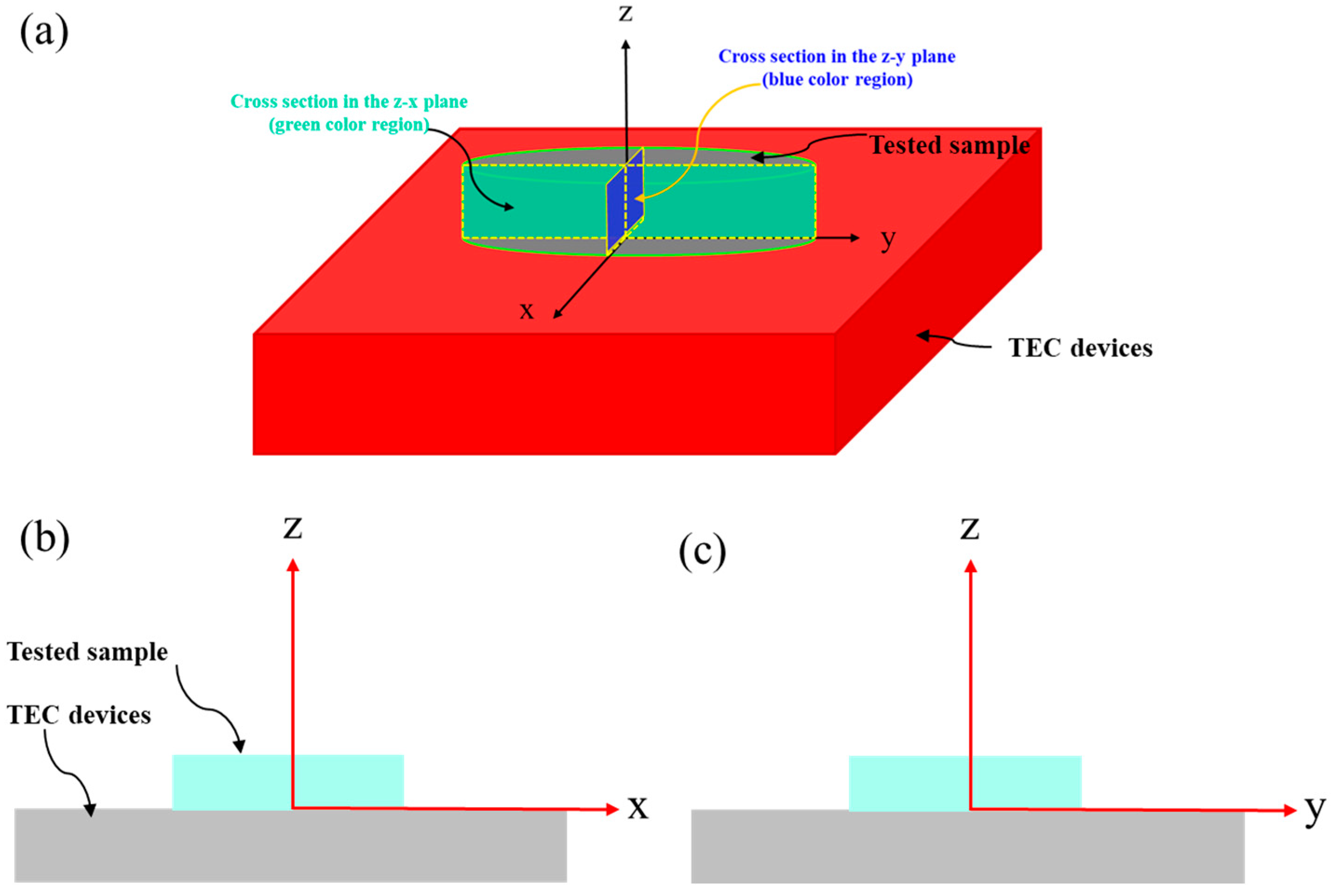
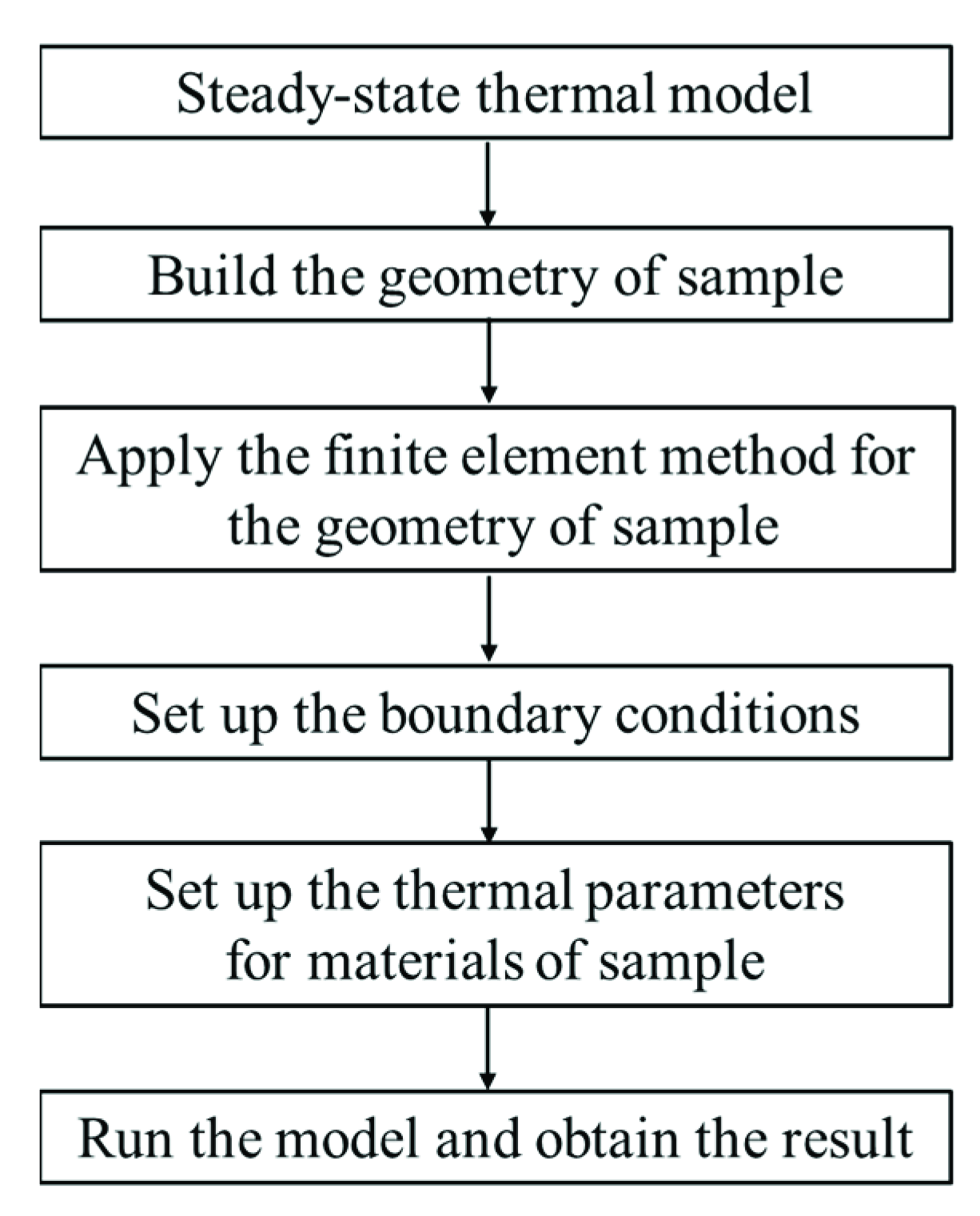
4. Simulation of Temperature Distribution

In addition to calculating the enhancement of thermal conductivity of the doped samples, it is also important to estimate the internal temperature distribution of the samples. In the case of heat transfer through the sample at a steady-state, temperature distribution can be easily obtained by applying the finite element method (FEM) and using MATLAB software to solve the heat diffusion equation with some known boundary conditions.
The symmetry property of sample geometry around the z-axis permits easy transfer of the problem of solving a heat diffusion equation in 3D into solving a heat diffusion equation in 2D. Temperature distribution in each plane of the cross-section is also symmetrical around the z-axis. The heat diffusion in 2D of the cross-section plane z–x can be written as
K ( 2 x 2 + 2 z 2 ) + q = 0
where K is thermal conductivity (W/m.K), and q is heat flux (W/m2). In the thermal steady-state, if the internal heat sources inside the sample are not significant, the heat diffusion equation is as follows
K ( 2 x 2 + 2 z 2 ) = 0
Figure 5a shows the 3D view of a sample placed on the TEC surface. The sample has the geometry of a thin cylinder. Rotating around the z-axis, different cross-section surfaces have the same shape as a rectangle which are the same size. Figure 5b,c illustrate the symmetry property of the cross-section at two planes, z–x and z–y, respectively. Figure 6 shows the application of the simulation procedure to the steady-state model to determine temperature distribution after simplifying the 3D model to a 2D model.
The steps in the simulation of temperature distribution are described in Figure 6. There are six main steps in this model. First, a steady-state thermal model is used in the MATLAB software. Second, the geometry of the TEC device and the tested sample are built using the corresponding code programming in the MATLAB software. The geometry parameters in the simulation are listed in Table 1. Third, the finite element method is applied to the geometry completed in the second step. Steps four and five are setting the boundary conditions and thermal parameters for the material of the test sample and the TEC device. These thermal parameters are listed in Table 2. The sixth and final step is to run the model code to obtain the result.
To illustrate the simulation process based on the steps in Figure 6, four cases of thermal conductivity improvement were simulated. The boundary conditions are set as follows: the temperature of the bottom surface of the test sample and the TEC’s hot surface is 100 °C; the temperatures of the top surface of the test sample are 50 °C, 62.5 °C, 75 °C, and 81.25 °C, corresponding to four cases of thermal conductivity improvement. Simulation results are shown in Figure 7 and Figure 8. Figure 7a shows the 2D geometry of the cross-section of the sample and TEC device created in the simulation. The bottom rectangle that is denoted as F1 is the cross-section of the TEC’s hot surface, which is bounded by edges E1, E2, E3, E7, E8, and E9. Domain F1 is 1 mm along the vertical axis, which is shown in the range 0 to 1 on the vertical coordinate’s axis. Domain F1 is 30 mm along the horizontal axis, which is shown in the range −15 to 15 on the horizontal coordinate’s axis. The sample is 0.5 mm thick and 16 mm in diameter, and is shown in the top smaller rectangle in Figure 7a. The cross-section of the sample is a rectangle that has a height of 0.5 mm and a width of 16 mm. In Figure 7a, the domain of this rectangle is denoted F2, and bounded by edges E4, E5, E6, and E8. Domain F2 is 0.5 mm along the vertical axis, which is shown in the range 1 to 1.5 on the vertical coordinate’s axis. Domain F2 is 16 mm along the horizontal axis, which is shown in the range −8 to 8 on the horizontal coordinate’s axis. Figure 7b shows the sample and the TEC device geometry by applying the finite element mesh. A mesh comprising the union of triangles is generated on the geometry of the test sample. The finite element used in the simulation is triangle geometry. To clearly illustrate the used finite element, a portion of meshed rectangle is enlarged, as shown in Figure 7b.
The simulation results for temperature distribution are shown in Figure 8, corresponding to 0.2 W/m.K, 0.3 W/m.K, 0.4 W/m.K, and 0.8 W/m.K. Results indicated that the higher enhancement of thermal conductivity caused a more uniform internal temperature distribution. Higher thermal conductivity will help heat transfer better; in other words, it reduces the heat isolate phenomena for samples with higher thermal conductivity. In Figure 8, the vertical axis shows the thickness of the sample while the horizontal axis describes the diameter of the sample. The thickness of the sample is 0.5 mm, which is shown in the range of 1.0 mm to 1.5 mm along the vertical axis. Meanwhile, the diameter is 16 mm, which is shown in the range of −8.0 mm to 8.0 mm along the horizontal axis. The values range is from −10 to 10 to help clearly show the output result of the simulation.
Another important consideration when conducting temperature simulations is that it is desirable to know the temperature values at each spatial position inside the sample. For that purpose, the simulation needs to interpolate temperature values and contour the temperature distribution across the sample. The corresponding simulation result is shown in Figure 9. The results show that at the position where the sample contacts the hot surface of the TEC device, temperature values are the same. However, the temperature of positions far away from the hot surface of the TEC device is proportional to the thermal conductivity enhancement of each sample. The sample with higher thermal conductivity enhancement showed a higher temperature value corresponding to the same spatial location across the thickness of the sample. This indicated that the enhancement of thermal conductivity can easily help transfer heat far away from hot regions.
The verification and validation of any proposed simulation model is an important requirement. The measurement of the spatial temperature distribution inside the sample is difficult because the thermal camera only shows the surface temperature. Furthermore, using the invasion method to detect the temperature is impossible for a thin sample. Therefore, the verification and validation of the proposed simulation model are accomplished by checking the reliability of the steps in the simulation model. First, the boundary condition is determined by the experiment before it is input into the programming code. The boundary is determined by experimentation using a thermal camera or thermocouple so that the detected temperature is verified. The steady-state thermal model is simpler than the nonsteady-state thermal model, as it only requires parameters including boundary temperature and thermal conductivity of the sample material. On the other hand, material parameters of thermal conductivity can be referred to from reliable studies, as well as based on the calculation of Equation (9), which uses data from experimental measurement. Although there are still some factors that affect the experimental temperature measurement process (such as variation in room temperature, setup emissivity parameter in the thermal camera during measurement, and contact between the sample and the TEC’s surface), the model can become reliable once the process determining the parameters for boundary conditions is well-considered and controlled as much as possible before being input into the simulation code.

5. Conclusions

Thermal conductivity enhancement of samples loaded with HTC fillers can be calculated based on the proposed mathematical model, which is derived from the theory of Fourier’s law. The change in thermal conductivity is calculated by determining the temperature difference between both surfaces of the sample without and with doping with HTC fillers. The formula to calculate thermal conductivity enhancement (TCE) of the sample with doping HTC was built and presented. An experimental setup was also presented to help calculate the thermal conductivity enhancement.
In addition to the mathematical model, a new idea and useful simulation method using MATLAB software were presented. The results indicate that we can apply MATLAB to find the solution for the question “How to simulate the spatial distribution of temperature in the sample?”
Temperature distribution can be easily visualized by the finite element method using MATLAB software. The 3D model can be simplified into a 2D model based on the symmetry property of sample geometry. The thermal model at a steady-state was built to find the temperature distribution corresponding to an improvement in thermal conductivity of the sample after fillers were added. An important step to make the model reliable is determination of the boundary temperature before inputting data into the simulation. Using a TEC device for heating samples made in the shape of a thin cylindrical plate and a thermal camera to determine the temperature at the bottom and top surfaces of the sample, the temperature to input as the boundary’s value in the steady-state model can be determined.
Temperature values are also easily interpolated to help estimate the changing temperature value corresponding to the space across the thickness of a sample after thermal conductivity is improved. The results show that when a sample’s thermal conductivity is enhanced, the temperature value increases for the same spatial location inside that sample. This indicates that the accumulation of heat will be reduced when the enhancement of thermal conductivity is improved.
The obtained results, which are based on the simple TEC device, thermal camera, and MATLAB software, indicate that the proposed method is meaningful due to its simplicity and cost efficiency, as it does not require expensive testing equipment and simulation software (e.g., COMSOL).

Author Contributions

Conceptualization, simulation, and writing—original draft preparation, Q.-K.N.; discussion, review, and editing, C.-C.T. All authors have read and agreed to the published version of the manuscript.

Funding

This research received no external funding.

Institutional Review Board Statement

Not applicable.

Informed Consent Statement

Not applicable.

Data Availability Statement

The data presented in this study are available on request from the corresponding author.

Conflicts of Interest

The authors declare no conflict of interest.

References

  1. Narendran, N.; Gu, Y. Life of LED-Based White Light Sources. J. Disp. Technol. 2005, 1, 167–171. [Google Scholar] [CrossRef]
  2. Lin, Y.-C.; Bettinelli, M.; Sharma, S.-K.; Redlich, B.; Speghini, A.; Karlsson, M. Unraveling the impact of different thermal quenching routes on the luminescence efficiency of the Y3Al5O12:Ce3+ phosphor for white light emitting diodes. J. Mater. Chem. C 2020, 8, 14015. [Google Scholar] [CrossRef]
  3. Davis, J.L.; Mills, K.-C.; Bobashev, G.; Rountree, K.-J.; Lamvik, M.; Yaga, R.; Johnson, C. Understanding chromaticity shifts in LED devices through analytical models. Microelectron. Reliab. 2018, 84, 149–156. [Google Scholar] [CrossRef]
  4. Singh, P.; Tan, C.-M. Degradation Physics of High-Power LEDs in Outdoor Environment and the Role of Phosphor in the degradation process. Sci. Rep. 2016, 6, 24052. [Google Scholar] [CrossRef] [Green Version]
  5. Ying, S.-P.; Fu, H.-K.; Tang, W.-F.; Hong, R.-C. The Study of Thermal Resistance Deviation of High-Power LEDs. IEEE Trans. Electron Devices 2014, 61, 2843–2848. [Google Scholar] [CrossRef]
  6. Górecki, K.; Ptak, P. Compact Modelling of Electrical, Optical and Thermal Properties of Multi-Colour Power LEDs Operating on a Common PCB. Energies 2021, 14, 1286. [Google Scholar] [CrossRef]
  7. Wang, Y.; Tang, B.; Gao, Y.; Wu, X.; Chen, J.; Shan, L.; Sun, K.; Zhao, Y.; Yang, K.; Yu, J.; et al. Epoxy Composites with High Thermal Conductivity by Constructing Three-Dimensional Carbon Fiber/Carbon/Nickel Networks Using an Electroplating Method. ACS Omega 2021, 6, 19238–19251. [Google Scholar] [CrossRef]
  8. Liu, Z.; Chen, Y.; Dai, W.; Wu, Y.; Wang, M.; Hou, X.; Li, H.; Jiang, N.; Lin, C.T.; Yu, J. Anisotropic thermal conductive properties of cigarette filter-templated graphene/epoxy composites. RSC Adv. 2018, 8, 1065. [Google Scholar] [CrossRef] [Green Version]
  9. Zheng, Z.; Dai, J.; Zhang, Y.; Wang, H.; Wang, A.; Shan, M.; Long, H.; Peng, Y.; Sun, H.; Chen, C. Enhanced Heat Dissipation of Phosphor Film in WLEDs by AlN-Coated Sapphire Plate. IEEE Trans. Electron Devices 2020, 67, 3180–3185. [Google Scholar] [CrossRef]
  10. Guo, L.; Zhang, Z.; Kang, R.; Chen, Y.; Hou, X.; Wu, Y.; Wang, M.; Wang, B.; Cui, J.; Jiang, N.; et al. Enhanced thermal conductivity of epoxy composites filled with tetrapod-shaped ZnO. RSC Adv. 2018, 8, 12337–12343. [Google Scholar] [CrossRef] [Green Version]
  11. Hao, W.; Li, L.; Chen, Y.; Li, M.; Fu, H.; Hou, X.; Wu, X.; Lin, C.; Jiang, N.; Yu, J. Efficient thermal transport highway construction within epoxy matrix via hybrid carbon fibers and alumina particles. ACS Omega 2020, 5, 1170–1177. [Google Scholar]
  12. Peng, C.; Zhang, G.; Sun, R.; Wong, C.P. Investigation of the optical properties of ZnO/epoxy resin nanocomposite: Application in the LED. In Proceedings of the 13th International Conference on Electronic Packaging Technology & High. Density Packaging, Guilin, China, 13–16 August 2012; pp. 376–379. [Google Scholar] [CrossRef]
  13. Shen, D.; Zhan, Z.; Liu, Z.; Cao, Y.; Zhou, L.; Liu, Y.; Dai, W.; Nishimura, K.; Li, C.; Lin, C.-T.; et al. Enhanced thermal conductivity of epoxy composites filled with silicon carbide nanowires. Sci. Rep. 2017, 7, 2606. [Google Scholar] [CrossRef] [PubMed] [Green Version]
  14. Ren, J.; Li, Q.; Yan, L.; Jia, L.; Huang, X.; Zhao, L.; Ran, Q.; Fu, M. Enhanced thermal conductivity of epoxy composites by constructing aluminum nitride honeycomb reinforcements. Compos. Sci. Technol. 2020, 199, 108304. [Google Scholar]
  15. Gaska, K.; Rybak, A.; Kapusta, C.; Sekula, R.; Siwek, A. Enhanced thermal conductivity of epoxy–matrix composites with hybrid fillers. Polym. Adv. Technol. 2015, 26, 26–31. [Google Scholar] [CrossRef]
  16. Rong, Y.; Su, F.; Zhang, L.; Li, C. Highly enhanced thermal conductivity of epoxy composites by constructing dense thermal conductive network with combination of alumina and carbon nanotubes. Compos. Part. A Appl. Sci. Manuf. 2019, 125, 105496. [Google Scholar]
  17. Kang, R.; Zhang, Z.; Guo, L.; Cui, J.; Chen, Y.; Hou, X.; Wang, B.; Lin, C.-T.; Jiang, N.; Yu, J. Enhanced thermal conductivity of epoxy composites filled with 2D transition metal carbides (MXenes) with ultralow loading. Sci. Rep. 2019, 9, 1–14. [Google Scholar] [CrossRef] [Green Version]
  18. Hu, J.; Huang, Y.; Zeng, X.; Li, Q.; Ren, L.; Sun, R.; Xu, J.; Wong, C. Polymer composite with enhanced thermal conductivity and mechanical strength through orientation manipulating of BN. Compos. Sci. Technol. 2018, 160, 127–137. [Google Scholar] [CrossRef]
  19. Kraemer, D.; Chen, G. A simple differential steady-state method to measure the thermal conductivity of solid bulk materials with high accuracy. Rev. Sci. Instrum. 2014, 85, 025108. [Google Scholar] [CrossRef]
  20. Braun Jeffrey, L.; Olson, D.; Gaskins, J.; Hopkins, P. A steady-state thermoreflectance method to measure thermal conductivity. Rev. Sci. Instrum. 2019, 90, 024905. [Google Scholar] [CrossRef] [Green Version]
  21. Santos, D.; Nunes, W. Thermal properties of polymers by non-steady-state techniques. Polym. Test. 2007, 26, 556–566. [Google Scholar] [CrossRef]
  22. Singh, A.K.; Panda, B.; Mohanty, S.; Nayak, S.; Gupta, M. Synergistic effect of hybrid graphene and boron nitride on the cure kinetics and thermal conductivity of epoxy adhesives. Polym. Adv. Technol. 2017, 28, 1851–1864. [Google Scholar] [CrossRef]
  23. Craddock, J.D.; Burgess, J.; Edrington, S.; Weisenberger, M. Method for direct measurement of on-axis carbon fiber thermal diffusivity using the laser flash technique. J. Therm. Sci. Eng. Appl. 2017, 9, 014502. [Google Scholar] [CrossRef]
  24. Chaudhry, A.U.; Mabrouk, A.N.; Abdala, A. Thermally enhanced polyolefin composites: Fundamentals, progress, challenges, and prospects. Sci. Technol. Adv. Mater. 2020, 21, 737–766. [Google Scholar] [CrossRef] [PubMed]
  25. Available online: https://www.comsol.com/heat-transfer-module (accessed on 19 April 2022).
  26. Available online: https://quickfield.com/transfer.htm (accessed on 19 April 2022).
  27. Available online: https://www.theseus-fe.com/simulation-software/heat-transfer-analysis (accessed on 19 April 2022).
  28. Available online: https://www.mscsoftware.com/application/thermal-analysis (accessed on 19 April 2022).
  29. Incropera, F.; Dewitt, D. Fundamentals of Heat and Mass Transfer, 5th ed.; Wiley: Hoboken, NJ, USA, 2002. [Google Scholar]
  30. Partial Differential Equation Toolbox for Use with MATLAB; The MathWorks, Inc: Natick, MA, USA, 1995.
  31. Heat Transfer. Available online: https://www.mathworks.com/help/pde/heat-transfer-and-diffusion-equations.html (accessed on 19 April 2022).
  32. Li, S.; Liu, J.-L.; Ding, L.; Liu, J.-X.; Xu, J.; Peng, Y.; Chen, M.-X. Active Thermal Management of High-Power LED Through Chip on Thermoelectric Cooler. IEEE Trans. Electron. Devices 2021, 68, 1753–1756. [Google Scholar] [CrossRef]
  33. Huang, B.J.; Chin, C.J.; Duang, C.L. A design method of thermoelectric cooler. Int. J. Refrig. 2000, 23, 208–218. [Google Scholar] [CrossRef]
Figure 1. Illustration of thermal conduction in one direction of z-axis.
Jcs 06 00214 g001
Figure 2. Simulation of improvement in thermo-conductivity of material corresponds to different values of n based on Equation (10).
Jcs 06 00214 g002
Figure 3. (a) Photo of TEC without operating and (b) temperature uniformity of TEC hot surface.
Jcs 06 00214 g003
Figure 4. (a) Determination of temperature of bottom and (b) top surfaces of sample.
Jcs 06 00214 g004
Figure 5. (a) A 3D view of the sample and the TEC illustrating the symmetry property of the sample and (b) the cross-section at the plane of z–x and (c) the plane of z–y.
Jcs 06 00214 g005
Figure 6. Steps in the steady-state model.
Jcs 06 00214 g006
Figure 7. (a) Block geometry of sample built in simulation (the unit of the vertical and horizontal axes is millimeters (mm)) and (b) sample geometry with finite element mesh and enlarged section.
Jcs 06 00214 g007
Figure 8. Simulation result of temperature for different cases of thermal conductivity enhancement: (a) K = 0.2 W/mK; (b) K = 0.3 W/mK; (c) K = 0.4 W/mK, and (d) K = 0.8 W/mK (the unit of the vertical and horizontal axes is millimeters (mm)).
Jcs 06 00214 g008
Figure 9. Simulation results of interpolate temperature and contour temperature distribution across the sample for different cases of thermal conductivity enhancement: (a) K = 0.2 W/mK; (b) K = 0.3 W/mK; (c) K = 0.4 W/mK; and (d) K = 0.8 W/mK (the unit of the vertical and horizontal axes is millimeters (mm)).
Jcs 06 00214 g009
Table 1. Geometry parameters in the simulation.
ValueUnit
Sample thickness0.5mm
Sample width (diameter)16mm
TEC device thickness5mm
TEC device width30mm
Table 2. Thermal parameter of material in the simulation. (The value of Ki will change depending on if the sample is without or with HTC filler).
ValueUnit
Sample thermal conductivityKiW/(m.K)
TEC device thermal conductivity130W/(m.K)
Publisher’s Note: MDPI stays neutral with regard to jurisdictional claims in published maps and institutional affiliations.

