
A Numerical Framework of Simulating Flow-Induced Deformation during Liquid Composite Moulding


Abstract
:1. Introduction
1.1. Background
1.2. Summary of Previous Work
1.3. Significance of the Present Work
2. Numerical Simulation Approach
- Develop a computational thermo-chemo-flow model that is capable of calculating the permeability, rheology, cure kinetics, and heat-transfer parameters of thermoset resins during the moulding of fibre preforms.
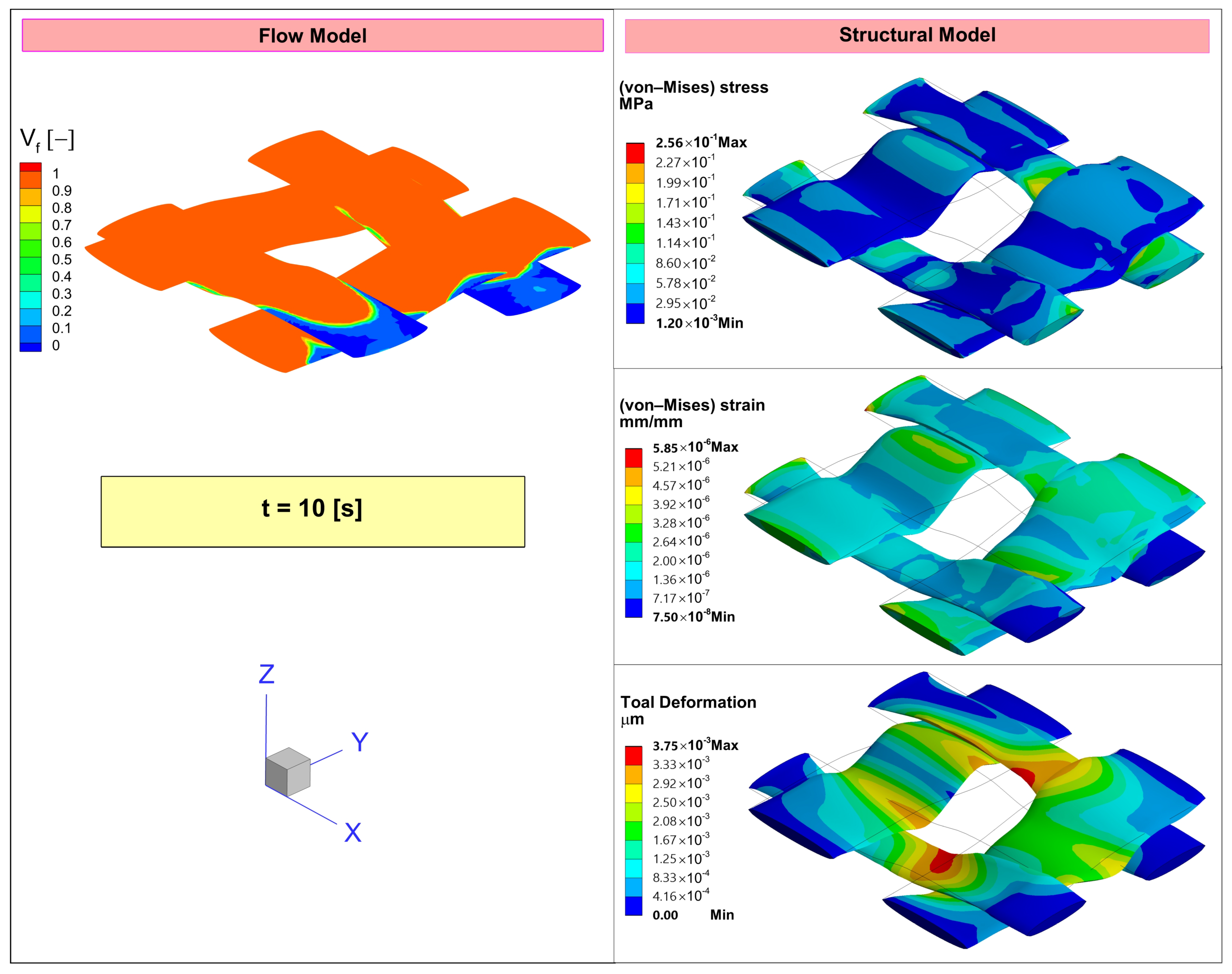
- Design a numerical one-way fluid–structure interaction (FSI) framework—linking CFD to FEA—to solve residual stresses/strains, and deformations of fibre bundles during fill and cure process cycles.
2.1. Thermo-Chemo-Flow Model
2.1.1. Flow Model
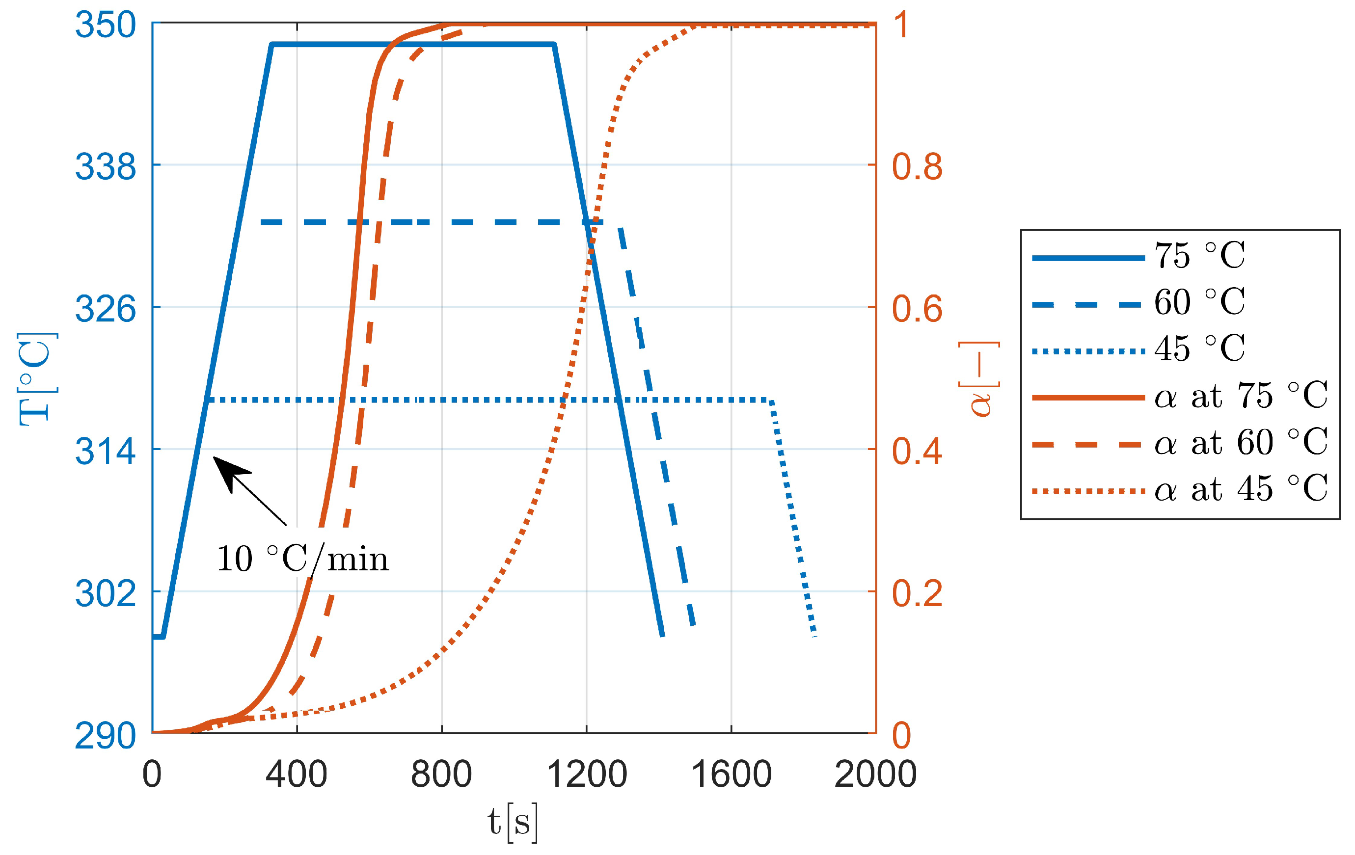
2.1.2. Heat Transfer and Cure Model
2.2. Structural Model
2.2.1. Deformation
2.2.2. Residual Stress and Strain
3. Results and Discussion
- Use of high-order upwind/interpolation schemes like second-order upwind and third-order MUSCL (Monotone Upstream-Centered Schemes for Conservation Laws)—for FVM analyses.
- Conversion (or transformation) of highly skewed cells (tetrahedral meshes) to polyhedral—for FVM analyses.
- Use of under-relaxation factors to control residuals (computed variables) at each iteration—for FVM analyses.
- Use of pinball radius to prevent penetration during deformation of solids (yarns) (controllable contacts)—for FE analyses.
4. Conclusions
Author Contributions
Funding
Data Availability Statement
Acknowledgments
Conflicts of Interest
Abbreviations
| Latin letters: | |
| Pre-exponential constant | |
| Specific heat | |
| Activation energy | |
| Young’s modulus | |
| Poisson’s ratios | |
| Shear modulus | |
| Model-dependent source term | |
| Gravitational acceleration | |
| H | Reaction heat |
| h | Yarn thickness |
| Thermal conductivity | |
| Permeability tensor | |
| Intra-tow permeability | |
| p | Pressure |
| Heat flux | |
| R | Universal gas constant |
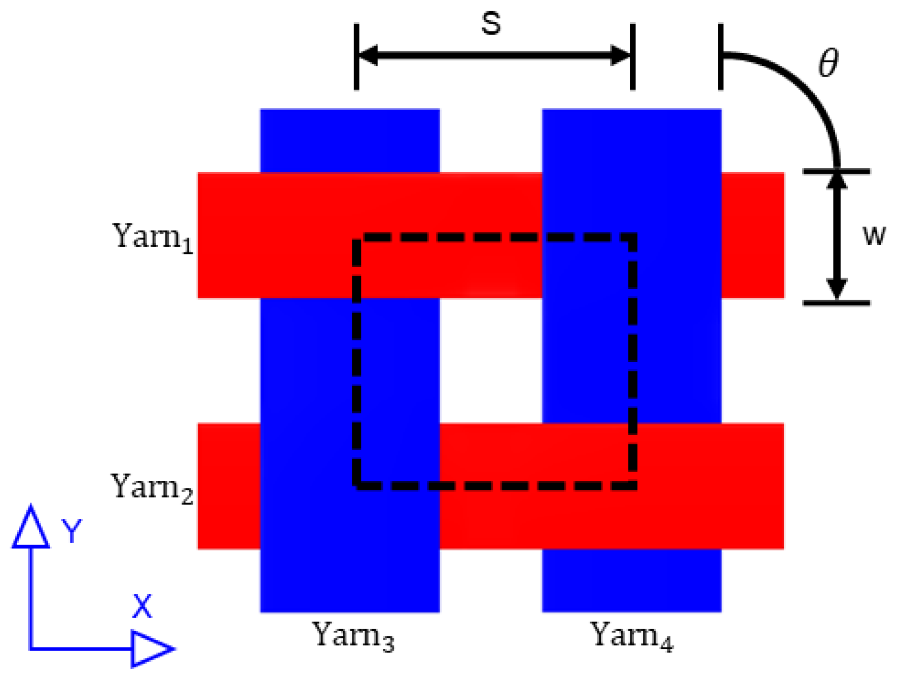
| S | Length of unit cell base |
| T | Temperature |
| Yarn/Tow width | |
| t | Time |
| Volume-averaged velocity | |
| Fibre volume fraction | |
| Weight fraction | |
| Greek letters: | |
| Rate of reaction | |
| Degree of cure | |
| Dynamic viscosity | |
| Density | |
| Porosity of the medium | |
| Nanofiller fraction | |
| Angle between warp and weft yarns | |
| Half period sinusoid of yarn cross-section | |
| Strain | |
| Engineering strain | |
| Stress | |
| Subscripts: | |
| ‖ | Longitudinal/parallel |
| ⊥ | Transverse/perpendicular |
| Equivalent (von)-Mises | |
| f | Fibre/filament |
| gel | Gelation point |
| o | Overall/global |
| r | Resin |
| s | Inter-tow/mesoscopic |
| t | Intra-tow/microscopic |
| x,y,z | Global coordinate system |
| Superscript: | |
| Exponents | |
References
- Alotaibi, H.; Abeykoon, C.; Soutis, C.; Jabbari, M. A numerical thermo-chemo-flow analysis of thermoset resin impregnation in lcm processes. Polymers 2023, 15, 1572. [Google Scholar] [CrossRef] [PubMed]
- Meola, C.; Boccardi, S.; Carlomagno, G.M. Chapter 1—Composite materials in the aeronautical industry. In Infrared Thermography in the Evaluation of Aerospace Composite Materials; Meola, C., Boccardi, S., Carlomagno, G.M., Eds.; Woodhead Publishing: Cambridge, UK, 2017; pp. 1–24. [Google Scholar] [CrossRef]
- Advani, S.G.; Sozer, E.M. 2.23—Liquid molding of thermoset composites. In Comprehensive Composite Materials; Kelly, A., Zweben, C., Eds.; Pergamon: Oxford, UK, 2000; pp. 807–844. [Google Scholar] [CrossRef]
- Kelly, A.; Zweben, C. Comprehensive composite materials. Mater. Today 1999, 2, 20–21. [Google Scholar] [CrossRef]
- Ermanni, P.; Di Fratta, C.; Trochu, F. Molding: Liquid composite molding(LCM). In Wiley Encyclopedia of Composites; John Wiley & Sons, Inc.: Hoboken, NJ, USA, 2012; pp. 1–10. [Google Scholar] [CrossRef]
- He, J.H.; He, C.H.; Qian, M.Y.; Alsolami, A.A. Piezoelectric Biosensor based on ultrasensitive MEMS system. Sens. Actuators Phys. 2024, 376, 115664. [Google Scholar] [CrossRef]
- Ma, Y.; Yang, Y.; Sugahara, T.; Hamada, H. A study on the failure behavior and mechanical properties of unidirectional fiber reinforced thermosetting and thermoplastic composites. Compos. Part B Eng. 2016, 99, 162–172. [Google Scholar] [CrossRef]
- Muzzy, J.D.; Kays, A.O. Thermoplastic vs. thermosetting structural composites. Polym. Compos. 1984, 5, 169–172. [Google Scholar] [CrossRef]
- Michaud, V. A review of non-saturated resin flow in liquid composite moulding processes. Transp. Porous Media 2016, 115, 581–601. [Google Scholar] [CrossRef]
- Gonçalves, P.T.; Arteiro, A.; Rocha, N.; Pina, L. Numerical analysis of micro-residual stresses in a carbon/epoxy polymer matrix composite during curing process. Polymers 2022, 14, 2653. [Google Scholar] [CrossRef]
- Yuan, Z.; Wang, Y.; Yang, G.; Tang, A.; Yang, Z.; Li, S.; Li, Y.; Song, D. Evolution of curing residual stresses in composite using multi-scale method. Compos. Part B Eng. 2018, 155, 49–61. [Google Scholar] [CrossRef]
- Dewangan, B.; Chakladar, N. Modelling of residual stress during curing of a polymer under autoclave conditions and experimental validation. Comput. Mater. Sci. 2024, 241, 113038. [Google Scholar] [CrossRef]
- Peng, X.; Xu, J.; Cheng, Y.; Zhang, L.; Yang, J.; Li, Y. An analytical model for cure-induced deformation of composite laminates. Polymers 2022, 14, 2903. [Google Scholar] [CrossRef]
- Kim, D.H.; Kim, S.W.; Lee, I. Evaluation of curing process-induced deformation in plain woven composite structures based on cure kinetics considering various fabric parameters. Compos. Struct. 2022, 287, 115379. [Google Scholar] [CrossRef]
- Fan, S.; Zhang, J.; Wang, B.; Chen, J.; Yang, W.; Liu, W.; Li, Y. A deep learning method for fast predicting curing process-induced deformation of aeronautical composite structures. Compos. Sci. Technol. 2023, 232, 109844. [Google Scholar] [CrossRef]
- Kuentzer, N.; Simacek, P.; Advani, S.G.; Walsh, S. Permeability characterization of dual scale fibrous porous media. Compos. Part A Appl. Sci. Manuf. 2006, 37, 2057–2068. [Google Scholar] [CrossRef]
- Hwang, W.R.; Advani, S.G. Numerical simulations of Stokes–Brinkman equations for permeability prediction of dual scale fibrous porous media. Phys. Fluids 2010, 22, 113101. [Google Scholar] [CrossRef]
- Parnas, R.S.; Salem, A.J.; Sadiq, T.A.; Wang, H.P.; Advani, S.G. The interaction between micro- and macro-scopic flow in RTM preforms. Compos. Struct. 1994, 27, 93–107. [Google Scholar] [CrossRef]
- Parseval, Y.D.; Pillai, K.M.; Advani, S.G. A simple model for the variation of permeability due to partial saturation in dual scale porous media. Transp. Porous Media 1997, 27, 243–264. [Google Scholar] [CrossRef]
- Gascón, L.; García, J.A.; LeBel, F.; Ruiz, E.; Trochu, F. A two-phase flow model to simulate mold filling and saturation in Resin Transfer Molding. Int. J. Mater. Form. 2016, 9, 229–239. [Google Scholar] [CrossRef]
- Happel, J. Viscous flow relative to arrays of cylinders. AIChE J. 1959, 5, 174–177. [Google Scholar] [CrossRef]
- Sangani, A.S.; Acrivos, A. Slow flow past periodic arrays of cylinders with application to heat transfer. Int. J. Multiph. Flow 1982, 8, 193–206. [Google Scholar] [CrossRef]
- Drummond, J.E.; Tahir, M.I. Laminar viscous flow through regular arrays of parallel solid cylinders. Int. J. Multiph. Flow 1984, 10, 515–540. [Google Scholar] [CrossRef]
- Gutowski, T.G.; Cai, Z.; Bauer, S.; Boucher, D.; Kingery, J.; Wineman, S. Consolidation experiments for laminate composites. J. Compos. Mater. 1987, 21, 650–669. [Google Scholar] [CrossRef]
- Gebart, B.R. Permeability of unidirectional reinforcements for RTM. J. Compos. Mater. 1992, 26, 1100–1133. [Google Scholar] [CrossRef]
- Cai, Z.; Berdichevsky, A.L. An improved self-consistent method for estimating the permeability of a fiber assembly. Polym. Compos. 1993, 14, 314–323. [Google Scholar] [CrossRef]
- Phelan, F.R.; Wise, G. Analysis of transverse flow in aligned fibrous porous media. Compos. Part A Appl. Sci. Manuf. 1996, 27, 25–34. [Google Scholar] [CrossRef]
- Woerdeman, D.L.; Phelan, F.R.; Parnas, R.S. Interpretation of 3-D permeability measurements for RTM modeling. Polym. Compos. 1995, 16, 470–480. [Google Scholar] [CrossRef]
- Castro, J.M.; Macosko, C.W. Studies of mold filling and curing in the reaction injection molding process. AIChE J. 1982, 28, 250–260. [Google Scholar] [CrossRef]
- Bruschke, M.V.; Advani, S.G. A numerical approach to model non-isothermal viscous flow through fibrous media with free surfaces. Int. J. Numer. Methods Fluids 1994, 19, 575–603. [Google Scholar] [CrossRef]
- Abbassi, A.; Shahnazari, M.R. Numerical modeling of mold filling and curing in non-isothermal RTM process. Appl. Therm. Eng. 2004, 24, 2453–2465. [Google Scholar] [CrossRef]
- Shojaei, A.; Ghaffarian, S.R.; Karimian, S.M.H. Modeling and simulation approaches in the resin transfer molding process: A review. Polym. Compos. 2003, 24, 525–544. [Google Scholar] [CrossRef]
- Antonucci, V.; Giordano, M.; Nicolais, L.; Di Vita, G. A simulation of the non-isothermal resin transfer molding process. Polym. Eng. Sci. 2000, 40, 2471–2481. [Google Scholar] [CrossRef]
- Liu, B.; Advani, S.G. Operator splitting scheme for 3-D temperature solution based on 2-D flow approximation. Comput. Mech. 1995, 16, 74–82. [Google Scholar] [CrossRef]
- Dessenberger, R.B.; Tucker, C.L. Thermal dispersion in resin transfer molding. Polym. Compos. 1995, 16, 495–506. [Google Scholar] [CrossRef]
- Kamal, M.R.; Sourour, S. Kinetics and thermal characterization of thermoset cure. Polym. Eng. Sci. 1973, 13, 59–64. [Google Scholar] [CrossRef]
- Sourour, S.; Kamal, M.R. Differential scanning calorimetry of epoxy cure: Isothermal cure kinetics. Thermochim. Acta 1976, 14, 41–59. [Google Scholar] [CrossRef]
- Kamal, M.R. Thermoset characterization for moldability analysis. Polym. Eng. Sci. 1974, 14, 231–239. [Google Scholar] [CrossRef]
- McBride, T.; Chen, J. Unit-cell geometry in plain-weave fabrics during shear deformations. Compos. Sci. Technol. 1997, 57, 345–351. [Google Scholar] [CrossRef]
- Wang, Q.; Yang, X.; Zhao, H.; Zhang, X.; Cao, G.; Ren, M. Microscopic residual stresses analysis and multi-objective optimization for 3D woven composites. Compos. Part A Appl. Sci. Manuf. 2021, 144, 106310. [Google Scholar] [CrossRef]
- Li, H.; Bacarreza, O.; Khodaei, Z.S.; Ferri Aliabadi, M.H. Probabilistic multi-scale design of 2D plain woven composites considering meso-scale uncertainties. Compos. Struct. 2022, 300, 116099. [Google Scholar] [CrossRef]
- Yang, N.; Zou, Z.; Potluri, P.; Soutis, C.; Katnam, K.B. Intra-yarn fibre hybridisation effect on homogenised elastic properties and micro and meso-stress analysis of 2D woven laminae: Two-scale FE model. Compos. Struct. 2024, 344, 118358. [Google Scholar] [CrossRef]
- Shojaei, A.; Ghaffarian, S.R.; Karimian, S.M. Three-dimensional process cycle simulation of composite parts manufactured by resin transfer molding. Compos. Struct. 2004, 65, 381–390. [Google Scholar] [CrossRef]
- Alotaibi, H.; Jabbari, M.; Abeykoon, C.; Soutis, C. Numerical investigation of multi-scale characteristics of single and multi-layered woven structures. Appl. Compos. Mater. 2022, 29, 405–421. [Google Scholar] [CrossRef]
- ANSYS Mechanical Enterprise. Engineering Data (Software ANSYS), Version 19.2; ANSYS, Inc.: Canonsburg, PA, USA, 2018.


| Description | Parameter | Units |
|---|---|---|
| Composite properties | ||
| Rheology | ||
| — | ||
| — | ||
| — | ||
| Cure kinetics | ||
| — | ||
| — | ||
| Parameter | Value | Parameter | Value |
|---|---|---|---|
| Width warp yarns | |||
| 50 | Gap warp yarns | ||
| 50 | Width fill yarns | ||
| 20 | Gap fill yarns | ||
| 37.5 |
| 0.2 | 0.4 |
| Injection Pressure | (von-Mises) Stress | (von-Mises) Strain | Total Deformation |
|---|---|---|---|
| 10 | 1.17 | 0.750 | |
| 50 | 5.85 | 3.75 | |
| 90 | 10.5 | 6.75 |
| Cure Temperature | Injection Pressure | (von-Mises) Stress | (von-Mises) Strain | Total Deformation |
|---|---|---|---|---|
| 45 | 10 | 1.57 | 2.69 | 8.10 |
| 50 | 40.0 | 71.7 | 210 | |
| 90 | 129 | 236 | 681 | |
| 60 | 10 | 1.58 | 2.70 | 8.15 |
| 50 | 40.4 | 72.1 | 212 | |
| 90 | 130 | 238 | 681 | |
| 75 | 10 | 4.89 | 8.93 | 25.5 |
| 50 | 40.8 | 72.4 | 213 | |
| 90 | 131 | 238 | 688 |
Disclaimer/Publisher’s Note: The statements, opinions and data contained in all publications are solely those of the individual author(s) and contributor(s) and not of MDPI and/or the editor(s). MDPI and/or the editor(s) disclaim responsibility for any injury to people or property resulting from any ideas, methods, instructions or products referred to in the content. |
© 2024 by the authors. Licensee MDPI, Basel, Switzerland. This article is an open access article distributed under the terms and conditions of the Creative Commons Attribution (CC BY) license (https://creativecommons.org/licenses/by/4.0/).
Share and Cite
Alotaibi, H.; Soutis, C.; Zhang, D.; Jabbari, M. A Numerical Framework of Simulating Flow-Induced Deformation during Liquid Composite Moulding. J. Compos. Sci. 2024, 8, 401. https://doi.org/10.3390/jcs8100401
Alotaibi H, Soutis C, Zhang D, Jabbari M. A Numerical Framework of Simulating Flow-Induced Deformation during Liquid Composite Moulding. Journal of Composites Science. 2024; 8(10):401. https://doi.org/10.3390/jcs8100401
Chicago/Turabian StyleAlotaibi, Hatim, Constantinos Soutis, Dianyun Zhang, and Masoud Jabbari. 2024. "A Numerical Framework of Simulating Flow-Induced Deformation during Liquid Composite Moulding" Journal of Composites Science 8, no. 10: 401. https://doi.org/10.3390/jcs8100401