Abstract
In this paper, specimens that contain cavities are tested and the critical force for crack initiation is compared to predictions made by the Coupled Criterion (CC). First, the material parameters Young’s modulus, Poisson’s ratio, fracture toughness, and critical stress are calibrated with tensile tests of three specimen shapes. Then, the critical force and crack initiation position are predicted for three other specimen shapes, called validation specimens. The predictions made by CC use stresses and incremental energy release rates that are computed by the Finite Element Method (FEM) and the Scaling Law based Meta Model (SLMM+AC). The predictions are validated against the tensile test results of the validation specimens. A Monte Carlo approach is used to compute prediction intervals for the critical force to make a statement about the quality of the predictions. The position of the crack initiation was predicted accurately, but the predicted critical loads deviated from the measured load up to 25%.
1. Introduction
To understand and predict the failure of composite materials on a fundamental level, it is necessary to develop modeling tools that are efficient and able to treat cracking phenomena near heterogeneities. As a first step, and taking heterogeneity to the extreme, voids inside a homogeneous material can be considered. The modeling tool must predict at which applied load and at what position on the void surface a crack will initiate, depending on the fracture parameters of the material. The failure model has to meet high requirements: it should accurately and efficiently predict the crack initiation for arbitrary voids with few specific material parameters.
Common failure models use the stress field computed by FEM simulations and check for every point on a cavity if the stress state is inside some failure surface [1]. However, these local failure models lack accuracy at sharp notches or even cracks, where the stress field approaches infinity. In such cases, sharp notches can be treated like cracks, and fracture mechanics provides a reasonable model [2]. The Theory of Critical Distances (TCD) works for both blunted and sharp cavities [3,4]. It uses the stress evaluated at a characteristic distance from the cavity and compares this stress to the material strength. The TCD assumes that the characteristic distance is a material parameter. However, this assumption is not plausible for all cases [5]. The Coupled Criterion (CC) instead combines stress- and energy-based criterion to compute the distance from the cavity such that both stress- and energy-criteria are fulfilled [5,6,7]. CC can accurately predict the crack initiation for cavities like V-notches [6,8,9,10,11,12] and circular holes [10,13,14,15,16], but CC requires the computation of the incremental energy release rate. This can be performed for relatively simple geometries by the Matched Asymptotic approach (MA) [17] or for more complex geometries by running FEM simulations for several crack increments, which we call the Full FEM approach. Since cavities in components may have complex geometries, the use of MA is limited and most times the position of the crack initiation position is not known in advance. In this case, Full FEM requires a number of FEM simulations for various positions to find the most critical position, and, hence, Full FEM requires too much computation time.
There is limited research on how to find the most critical position where a crack will initiate. Li and Leguillon suggested a method that is based on a watershed floating process [18]. For components with several bolts used to repair a composite panel, a two-stage approach was presented that finds the most critical hole introduced for the bolts [15]. Furthermore, the Phase field approach can be used to mimic the CC criterion [19].
In this paper, a Scaling Law-based Meta Model with Auto-Controlled boundary conditions (SLMM+AC) [20] is used to predict the incremental energy release rate efficiently such that CC can be applied to various positions at a cavity. For this, SLMM+AC fits a precomputed cell to match the cavity surface and the displacement field computed by one single FEM simulation. Since only one simulation is required, SLMM+AC is very efficient. For a detailed description of the SLMM+AC method, the reader is referred to a previous paper [20].
It needs to be shown whether our approach of using CC in common with SLMM+AC is able to transfer results of calibration tests to other validation specimens that include arbitrary shaped notches. It has been shown that the CC it is well suited to account for length scale effects [5] that were previously described for quasi-brittle materials by Bazant’s scaling law [21]. Our hypothesis is that the critical load and the position of crack initiation are predicted efficiently and accurately for the validation specimens.
To prove this hypothesis, six specimen shapes with five repetitions each were laser-cut out of a polymethyl methacrylate (PMMA) plate. Three of the shapes were used to obtain the Young’s modulus and Poisson’s ratio, the critical energy release rate, and the critical stress of the material, respectively. Further, three specimen shapes were used to validate our SLMM+AC approach by predicting the most critical position and the critical load for the validation specimens. The predictions are compared to the predictions of the Full FEM approach and the measured critical loads. To account for the scatter of material properties and possible shape variations, distributions of Young’s modulus, critical energy release rate, and critical stress are computed from the tests. With these distributions, a prediction interval for the critical load in the validation specimens is computed using a Monte Carlo (MC) method.
2. Materials and Methods
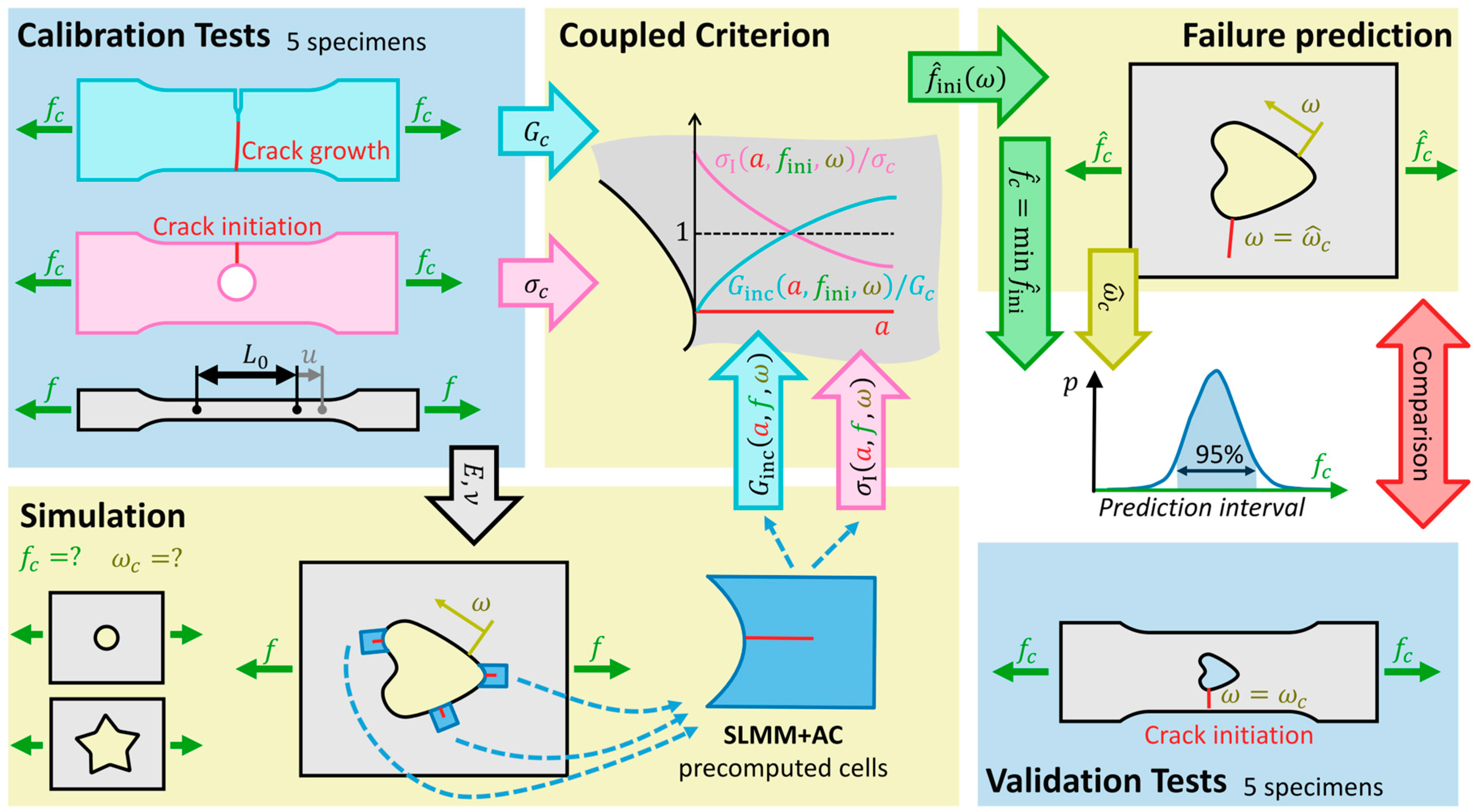
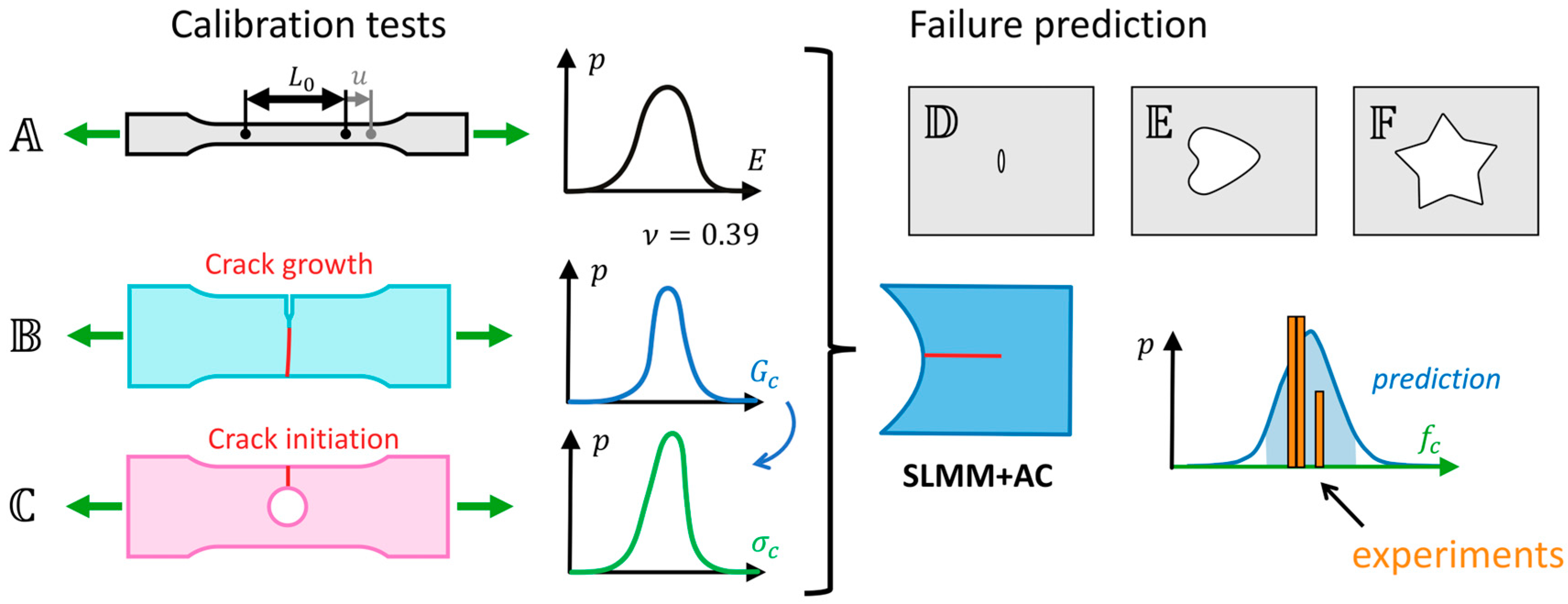
The aim of this paper is to transfer results from calibration tests to validation specimens and to correctly predict the critical load and the position of a crack initiation for the validation specimens. The predictions are then compared to the test results of the validation specimens. Figure 1 shows an overview of this procedure: The calibration tests provide the material parameters . The validation specimens are simulated using to obtain the strain fields. SLMM+AC computes and at various positions of the cavity using from the calibration tests to predict the initiation load at various positions . Next, the most critical position and the corresponding critical load are determined and a prediction interval is computed. The results of the validation tests are then compared to the predictions.
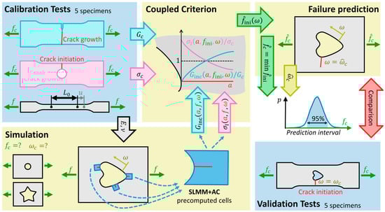
Figure 1.
Procedure for the tests (light blue background) and evaluation (light yellow background) with predicted initiation load and comparison between them (red arrow).
To obtain the critical incremental energy release rate or fracture energy , the critical stress , the Young’s modulus and the Poisson’s ratio , the three specimen shapes –, see Figure 2, are used as calibration tests. The other three specimen shapes, –, also shown in Figure 2, are used for the validation. For these validation specimen shapes, simulations are performed and the incremental energy release rate and the (in-plane) major principal stress are computed by SLMM+AC for various positions at the cavity surface. In cases where SLMM+AC is not applicable, additional Full FEM simulations are carried out to compute and .
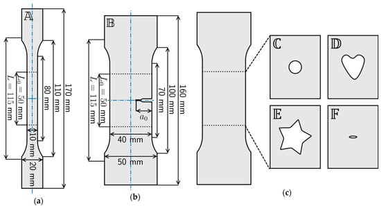
Figure 2.
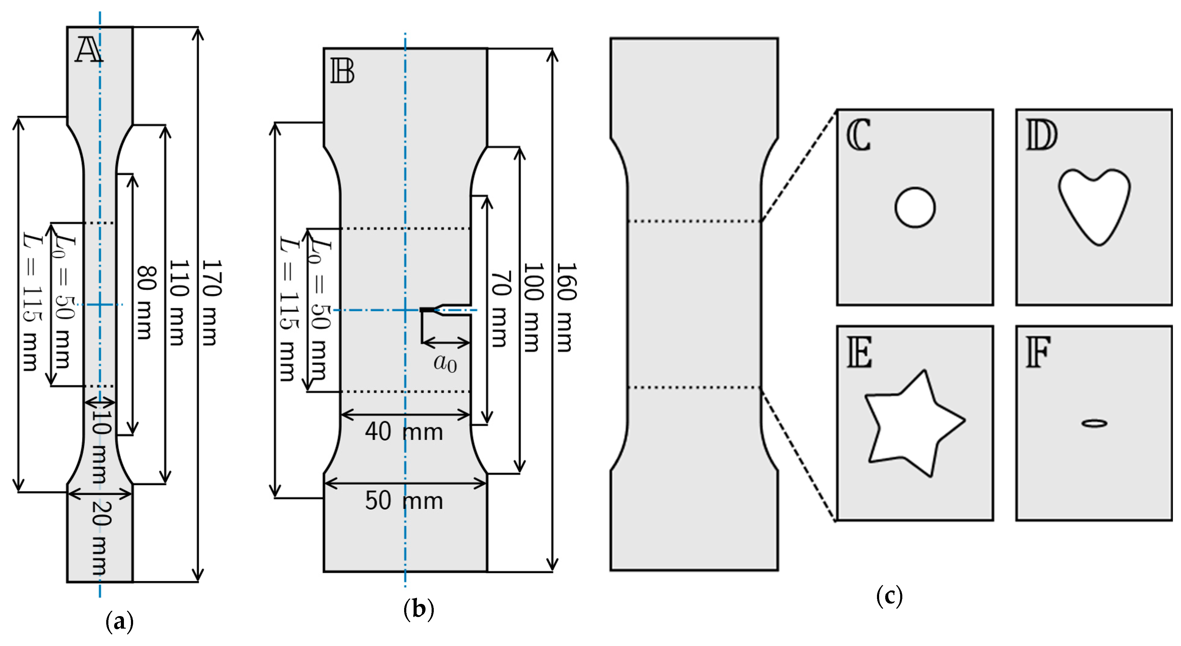
Specimen shapes used in this study: (a) type 1B [22], (b) SENT [2], and (c) specimens that contain cavities. The specimen shapes are used for the calibration. The specimen shapes are used for the validation. The region surrounded by dashed lines is the measurement region for the DIC. In this region the displacement is determined. The clamping length is .
Given the calibrated quantities and and the computed quantities and , the Coupled Criterion (CC) predicts a load at which a crack should initiate at a position . Note that, in tests, the force and the specimen thickness are measured. The load is defined as follows:
Next, the most critical load and position are found. For the most critical load, a prediction interval is computed using a Monte Carlo (MC) method. The predicted critical load and position are compared to the critical load and position measured in tensile tests.
2.1. Specimen Shapes
Figure 2 depicts six specimen shapes –. For each specimen shape, five samples are manufactured and tested. is the clamping length and is the region where the displacement is measured. Specimen corresponds to a multi-purpose specimen of type 1B according to the standard DIN EN ISO 527-2 [22]. Specimens – have the same outer shape of single-edge notched tension (SENT) specimens [2], with corresponding to a SENT specimen with an initial crack, and – without an initial notch and crack but with a cavity of varied shape:
- contains a circular cavity at the center of the specimen with a radius .
- contains a heart-shaped cavity with a width of and a height of , see Figure 2c.
- contains a star-shaped cavity whose corners are blunted by a radius .
- contains an elliptical cavity with a width of and a height of .
2.2. Experimental
2.2.1. Material and Sample Preparation
For the validation of the model, commercially available polymethyl methacrylate (PMMA), with the brand name PLEXIGLAS® XT, from Thyssenkrupp (thyssenkrupp Plastics GmbH, Essen, Germany), in sheet form (thickness approx. 4 mm) was used. The outer geometries shown in Figure 2 were cut using a CO2 laser from Trotec Laser GmbH (SPEEDY 100, Trotec Laser GmbH, Austria). The laser power was 50 W and the cutting speed was approx. 13 mm/s. The cavities in specimen shapes – were cut in the same way.
Before deciding to use the laser to cut the cavities, conventional drilling and waterjet cutting were tested. Both were rejected. Drilling introduced unacceptable residual stresses in large areas of the specimen, as observed with the photo-optical method. In addition, the diameter of the water jet beam increases with distance from the nozzle, making it impossible to produce a uniform cavity across the thickness of the specimen.
The samples of type correspond to a single-edge notched tension (SENT) specimen [2], whereby only the outer contour was cut out using a CO2 laser. Both the machine and the sharp notch were subsequently introduced. A conventional Leica RM2255 microtome (Leica Mikrosysteme GmbH, Austria) was used for this purpose, equipped with a razor blade to introduce a uniform sharp notch via a smooth sliding movement. The ratio of the initial crack length to specimen width ( ratio) was chosen to be about 0.3. Before testing, all samples were primed white in a further step and provided with a fine black spray pattern to enable measurement of the specimen deformation using digital image correlation (DIC).
2.2.2. Testing
All tests were performed using a Zwick Z250 universal testing machine (ZwickRoell GmbH & Co. KG, Germany). This was equipped with a 10 kN load cell and 10 kN mechanical clamping jaws. The displacement measurements were carried out using DIC in the measurement region . An Allied Vision Prosilica 6600 GT camera (Allied Vision Technologies, Germany) equipped with a Tokina AT-X 100 mm 2.8 Pro D lens from Keno Tokina Co., Ltd. (Japan) was used for this purpose. The measurements were evaluated using the Mercury RT system (Sobriety s.r.o., Kuřim, Czech Republic) with software version v2.9x64, whereby the gauge length was set to (see Figure 2) for all specimens (–).
Specimen was used to determine Young’s modulus and Poisson’s ratio. A clamping length of was used for this measurement. The loading rate was 1 mm/min up to an elongation of 0.25%, as specified in DIN EN ISO 527-2 [22]. After that, the loading rate was switched to 10 mm/min until a fracture occurred. Specimen geometry was used to determine the fracture toughness. Again, a clamping length of 115 mm and a loading rate of 10 mm/min was used. After fracturing the samples, was determined using a VHX-7000 digital light microscope from Keyence (KEYENCE Corporation, Japan) in reflected light mode. No detailed analysis of the fracture surfaces (such as studies of crack surface topography [23]) or the crack propagation velocities [24] was performed. Samples – were tested using the same clamping length and loading rate. A total of five repetitions was carried out for each geometry, –.
2.3. Evaluation
2.3.1. FEM Models
Figure 3 depicts FEM models of specimens with a crack or a cavity. The models cover the clamped region with a length . A constant load is applied at the top reference point (orange cross). The models use the small strain framework and a linear elastic material defined by a Poisson’s ratio and a Young’s modulus of . The linear character allows for the scaling of the results afterward to the actual load and Young’s modulus. The Poisson’s ratio is calibrated as described in Section 2.3.3. Since the specimen thickness is small, we assume plane stress conditions.
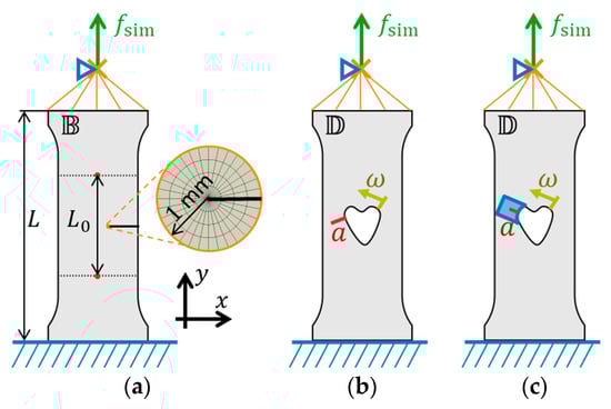
Figure 3.
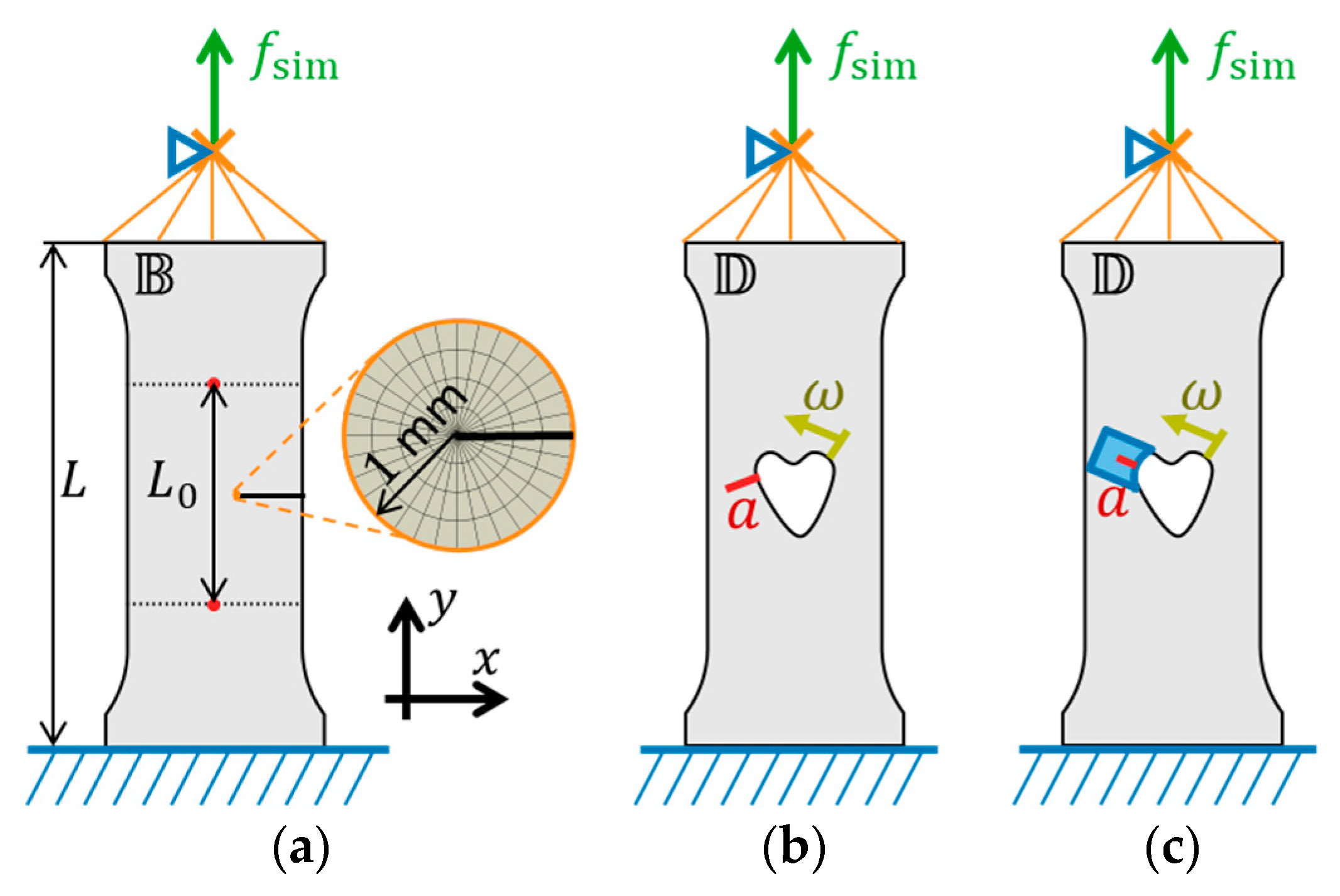
The FEM models are loaded with , which is applied at a reference point. (a) For the SENT [2] setup of specimen shape , a crack tip mesh with collapsed elements is used. (b) The Full FEM approach with specimen shape needs to introduce cracks and perform several FEM simulations. (c) The SLMM+AC approach with specimen shape instead uses precomputed cells that are fitted to the notch surface.
A kinematic coupling connects all degrees of freedom of the top reference point with the top edge of the models. The bottom side is fixed. The models are meshed using 2D triangular and reduced integrated rectangular elements with quadratic shape functions and plane stress formulation (CPS8R and CPS6). The mesh size is set to 0.2 mm, which corresponds to about 575 elements over the model length.
Figure 3a depicts the meshed crack tip for geometry . The stress singularity at the crack tip is approximated using collapsed rectangular elements whose midside node is shifted 25% to the crack tip [25].
The specimens – contain cavities. Figure 3b,c depicts as a representative model of the other specimens. Cracks initiate at a position on the cavity surface for a given model . Since is not known a priori, we introduce trial cracks at every position and test which position is the most critical one. To do so, the major principal stress and the incremental energy release rate are computed over the trial crack path for every position . The control variable defines the location along the crack initiation paths. We implement two approaches to obtain and : the Full FEM approach and the Scaling Law based meta model approach SLMM+AC [20].
The first approach, called Full FEM, introduces a trial crack at some position as depicted in Figure 3b. The major principal stress is extracted from the FEM simulation without a trial crack. The superscript FE stands for Full FEM. To evaluate , the nodes along the trial crack are sequentially opened up to a length and the displacement of the reference point is computed. With the displacement without the crack, the incremental energy release rate is computed as follows:
Appendix A describes how to derive Equation (2). The Full FEM approach does not use a special crack tip mesh.
The second approach, called SLMM+AC, was introduced by Rettl et al. [20] and fits a precomputed cell to a position at the cavity, as shown in Figure 3c. The curvature and the cell size are varied such that the cell matches the cavity surface, and the cell size is maximized up to a cell height of 4 mm. The cell contains the trial crack and predicts and with just one simulation of the uncracked geometry. For a detailed explanation we refer to Rettl et al. [20]. The prediction is only possible up to a maximum trial crack length , which is limited by the SLMM+AC approach and depends on the cell height.
As mentioned above, the linear elastic material model and the small strain framework allow for the results to be scaled to the actual Young’s modulus and load . The major principal stress
is scaled by the load . The incremental energy release rate
is scaled by the load and the Young’s modulus .
2.3.2. Coupled Criterion (CC)
The Coupled Criterion (CC) [6] predicts the initiation load needed for a crack to initiate from the cavity surface of an arbitrary geometry . To apply CC, trial cracks are introduced at various positions normal to the surface. Figure 4a shows a trial crack of length . For a given position , Young’s modulus , and geometry , CC requires computed values and as well as two material parameters: The critical stress and the fracture energy . The material parameters are calibrated as described in Section 2.3.3.
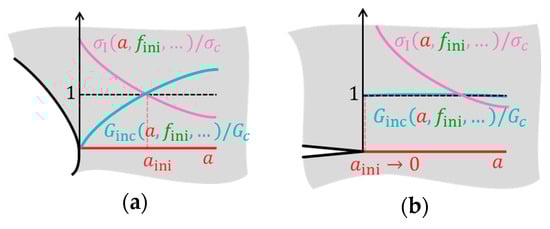
Figure 4.
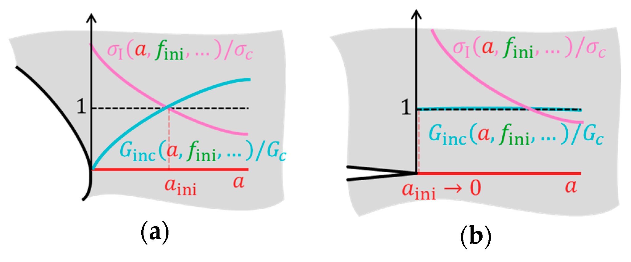
The Coupled Criterion states that a crack initiates at the lowest possible load , at which an energy criterion (turquoise) and a stress criterion (pink) are both fulfilled at one point . (a) For a blunted notch CC computes the intersection of the stress and energy criterion with the dashed line at 1. (b) In front of a crack the stress criterion is always fulfilled and just the energy criterion is considered.
According to CC, a crack initiates if a stress and an energy criterion are fulfilled simultaneously. According to the stress criterion (pink), a crack of length initiates when along the whole trial crack path up to . According to the energy criterion (blue), a crack of length initiates when . Furthermore, a crack initiates at lowest load that fulfills both of the following criteria:
Equation (5) can be either used to find for given or to find for given . The latter is used for the calibration of the material parameters as described in the next section. Note that CC uses a homogenized material, which means that the effect defects on a smaller length scale than the notch investigated are included in the critical stress , which may differ from the material strength [26].
For a sharp crack, as depicted in Figure 4b, CC approaches the linear elastic fracture mechanics. At the crack tip, the stress approaches infinity; hence, the stress criterion is always fulfilled. The incremental energy release rate is constant, because, after the crack grows by some , it is still a crack with similar loading conditions. Consequently, a crack will “initiate” or grow with a very small increment . The incremental energy release rate is computed from the strain energy and approaches the energy release rate known from fracture mechanics:
2.3.3. Statistics
To account for the scatter in the material properties, we introduce probability distributions for the Young’s modulus , the critical energy release rate , and the critical stress . These distributions are calibrated against the experimental data: see Figure 5. The fast SLMM+AC method then allows for the use of a Monte Carlo analysis that provides the prediction intervals of the failure load in the three validation specimens , , and .
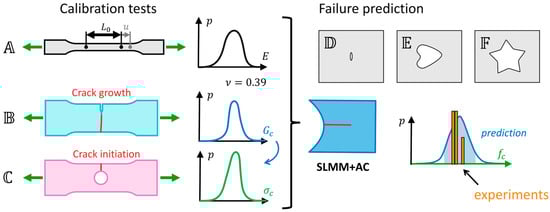
Figure 5.
The method of the statistical analysis: Calibration tests with specimen shapes , , and provide probability functions for the Young’s modulus , fracture energy , and the critical stress . A Monte Carlo approach uses the SLMM-AC method to obtain a prediction interval of the failure load from these material parameter distributions. This prediction interval is then compared to the experimental results of the validation specimens , , and .
In this section, the terms necessary for the statistics are defined, followed by a description of how probability distributions of material properties are fitted. Finally, details of the calculation of the prediction intervals of are given.
To provide a statistical evaluation, we use terms like specimen shapes, tests, random variables, estimators, and true values. A specimen shape is denoted in upper case blackboard bold (e.g., ). It defines the geometry and is used as representative of the (statistical) population of all tests with this geometry. A test (e.g., ) is denoted in lower case blackboard bold. A test is an event in the statistical sense, and it is a sample of the corresponding population . A quantity that is measured during a test or computed from such measurements is denoted a random variable in the statistical sense and is printed in bold. Given a set of tests , the mean value and the sample standard deviation of a quantity might be computed. and are estimators for the true mean value and population standard deviation . Another estimator type (e.g., ) predicts, based on observed tests a quantity for an unobserved test that is marked by a tilde. As a shortcut, we write .
Furthermore, random variables like can be used to create a probability distribution. A cumulative probability function
is defined as the probability of being smaller or equal to some given . A probability density function
is the derivative of the cumulative probability function with respect to . A prediction interval of
can be defined by the -quantiles and the -quantile .
2.3.4. Parameter Calibration
The parameters , , and are calibrated against the tests . Figure 2 shows the specimen shapes that correspond to those tests. Grubbs’ (statistical) test [27] with a significance is used to detect (tensile) tests that are outliers. Such (tensile) tests are excluded from the further analysis.
The Young’s modulus and the Poisson’s ratio are evaluated for all tests . The Young’s modulus is computed according to DIN EN ISO 527 [22]. The Poisson’s ratio is computed from the DIC results.
The fracture toughness is evaluated for all tests with the help of the FEM model depicted in Figure 3a. The critical load and the initial crack length are measured for each test . The initial crack with a length is introduced in the FEM model and the J-Integral [28] is computed around the fourth contour, which is indicated by an orange circle in Figure 3a. The fracture toughness
depends only on the test . Note that Anderson [2] provides a simple analytical equation for the fracture toughness for SENT specimens. However, Anderson assumes that the specimens can freely rotate whereas the rotation in the tested specimens is prevented by the clamps.
The critical energy release rate for plane stress
depends on both the fracture toughness and the Young’s modulus. As shown in Equation (6), the fracture energy is used by CC for the comparison with the incremental energy release rate.
To obtain the critical stress, Equation (5) of CC is used for the elliptical cavity in geometry . For the calibration, a trial crack is introduced at the right of the ellipse (), and and are computed using the Full FEM approach with the Young’s modulus , fracture energy and the critical load of geometry . Next, Equation (5) is used to find the critical stress that depends on , and .
2.3.5. Failure Prediction
The hypothesis of this paper is that we can predict the critical position and the critical load for the validation geometries depicted in Figure 2. For the prediction, the measured values from the calibration tests - are averaged to , , , and . The average fracture energy and critical stress are computed as described in Section 2.3.4 using the other averaged values.
Given an arbitrary geometry and material parameters , , , and , Equation (5) is used to estimate the initiation load and initiation length for every position at the cavity. To prevent additional simulations, SLMM+AC is used to predict both the incremental energy release rate and the major principal stress. SLMM+AC provides predictions only up to a maximum crack length , which is a model parameter of SLMM+AC. If the crack length is larger than , the initiation load cannot be computed. However, since the stress criterion has to be fulfilled over the whole initiating crack up to , it is obvious that holds true for . The most critical case would be the smallest possible load that still fulfills this requirement. This load is computed such that . We take as lower bound for the initiation load at positions where SLMM+AC is not applicable otherwise.
The most critical position is the position where the crack initiates at the lowest initiation load . To find the most critical position, all positions are split into applicable positions and not applicable positions . A position is not applicable if . First, the smallest initiation load of all applicable positions is computed. Next, we check if a not applicable position might be more critical. This is the case for all with . All applicable positions with and all not applicable positions with are marked as potential critical positions. For these potential critical positions, additional simulations are performed, and the initiation load is computed based on the Full FEM approach. The smallest of those initiation loads is considered to be the critical load and the corresponding position is the critical position at which we expect a crack to initiate.
2.3.6. Prediction Interval
To determine a prediction interval for the critical load , the position is held constant at the value computed in the previous section. We assume that the observed uncertainty is only due to material scattering. Every material piece has its own Young’s modulus , fracture toughness , and critical load that are assumed to be independently normally distributed with mean values and standard deviations . The tilde marks that the tests are future realizations that are observed just indirectly, because a material piece can be tested only once to obtain either the Young’s modulus or the fracture toughness or the critical load or another critical load for an arbitrary specimen shape . Since the validation specimens are tests for to provide , the quantities , , and are unknown and have to be estimated somehow.
For this, we approximate the unknown mean values and unknown standard deviations by the mean values and sample standard deviations of the tests -. Next, a random variable for a future realization of the Young’s modulus
is defined with a Student’s -distributed random variable [29]. Student’s distribution has degrees of freedom and arises if mean and standard deviation are estimated [30]. is the number of observed tests in . The same approach is used for the fracture toughness
for an unobserved test , where tests are observed. The critical load
for an unobserved test bases again on observed tests . Note that , , and are assumed to be independent random variables. As a shortcut, we write , , and . The random variables , , and are used to define probability density distributions , , and as described in Section 2.3.3.
Next, a Monte Carlo method [31] is used to compute the probability distribution of the critical stress and, subsequently, the critical loads for the validation tests. For this, vectors are randomly sampled using Equations (12)–(14). For each vector the fracture energy and the critical stress are computed as described in Section 2.3.3.
The cumulative probability distribution for a future realization of the critical stress is generated by counting how many sampled critical stresses are smaller than or equal to . Since this is a discrete operation, the probability density function cannot be constructed from the derivative of the discrete as described by Equation (8). Instead, a Gaussian kernel density estimation [32] is used to generate the probability density function from the sampled data.
Next, the critical loads for the validation tests are predicted using Equation (5) with the quantities from the sampled vector and the computed critical stress . The Full FEM approach predicts the incremental energy release rate and the major principal stress.
Like for the critical stress, the probability density functions are constructed using a Gaussian kernel density estimation. With the known probability distribution, the prediction interval for the critical load is defined as follows:
Next, we check whether the observed critical loads from the realized validation tests are inside the prediction interval.
3. Results and Discussion
In the following, the results of the experiments and models for the calibration tests (specimen shapes –) are presented. The experimental results are then compared with the predictions of our CC-based SLMM+AC method for the validation tests (specimen shapes –.).
Figure 6 depicts the measured load–displacement curves (orange) of all six specimen shapes with five specimens. The gray horizontal lines represent the critical force for each sample. In addition, simulated load–displacement curves are plotted as blue curves, using the specimen shapes (for specimen shape , taking into account the initial crack length of each specimen) with mean material parameters as computed from specimen shape tests, see Section 3.1. This allows for a comparison of the stiffness between experiment and simulation and the validity of using a linear-elastic material model in the simulations.
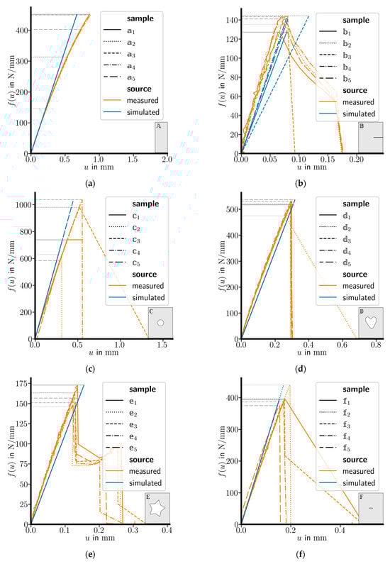
Figure 6.
Load–displacement curves from tensile tests (measured) and FEM simulations (simulated) for specimen shapes (a) , (b) , (c) , (d) , (e) , and (f) . The geometries of the specimens were also used for the simulation curves, which explains the variations in the specimen shape , where the initial crack length varied. The sample was excluded from the analysis.
Figure 6a shows the load–displacement curve for the tensile test of . The measured curves considerably deviate from the simulated ones above , which corresponds to a strain . The maximum strains observed in the simulations of other specimens are (), (), (), and (). However, most simulated load–displacement curves are in good agreement with the measured curves, as can be seen in Figure 6c–f. Furthermore, only slight nonlinearities can be observed in the experimental curves of specimen shapes , , and , which means that the nonlinear effects are confined to smaller regions of the specimens. To allow for the scaling in SLMM+AC, we stick to linear elastic material behavior and assume that, if this linear model is also used for calibration, the predictions can still be accurate. In Figure 6b, all curves are plausible except for sample , which is marked as an outlier in Table 1. Note that, for specimen shape , the initial crack length is measured for each specimen and causes the variation in stiffness of the simulation curves in Figure 6b.

Table 1.
Measured and computed quantities for all tested samples. [a] Statistical outliers and [b] invalid tests broken at the clamps are not used for the further computation.
Table 1 lists the measured and derived quantities for all tested samples. Additionally, the mean values and sample standard deviations are provided. As already mentioned, the failure prediction uses the mean values , , , and . Note that is more than 10 standard deviations higher than the mean value and is considered an outlier. The sample is printed in bold and is excluded from the further evaluation. Consequently, for only valid tests are available. The tests and are invalid and excluded, because the crack initiated at the clamp. This reduced the number of valid tests for to . All other specimen shapes have five valid tests.
Remember that our SLMM+AC approach is based on 2D models, meaning that a drop in force is associated with a crack initiation and propagation uniformly over the specimen thickness. In the experiments, however, the crack typically initiates from an initial defect and then grows radially from there. This is indicated in Figure 7 for the specimen (circular hole), which shows the fracture surface of the ligament that fractured first. The fracture surface shows initial conical markings (radial lines inside the semicircle—see figure closeup) starting from the crack initiation point. In fundamental studies of fractures in PMMA [33,34], such conical markings were correlated with PMMA fracture toughness, temperature, and loading rate. In addition, the gradient in the white areas indicating crazes in the material was explained by changes in crack-driving forces and, therefore, crack growth rates. This actual radial fracture process can explain additional scatter in the tested critical loads of the specimens and limit the transferability of material parameters calibrated for a specific specimen thickness to other thicknesses.
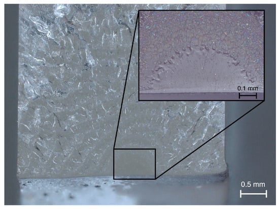
Figure 7.
Fracture surface of specimen (the ligament where the fracture started). The semi-circular crack initiation is clearly visible at approximately 60% of the specimen thickness and shows initial conical markings typical of PMMA. This initiation is followed by unstable crack growth, with white areas indicating crazing and hence plastic deformation. A slight irregularity in the laser cut is also visible.
3.1. Calibration
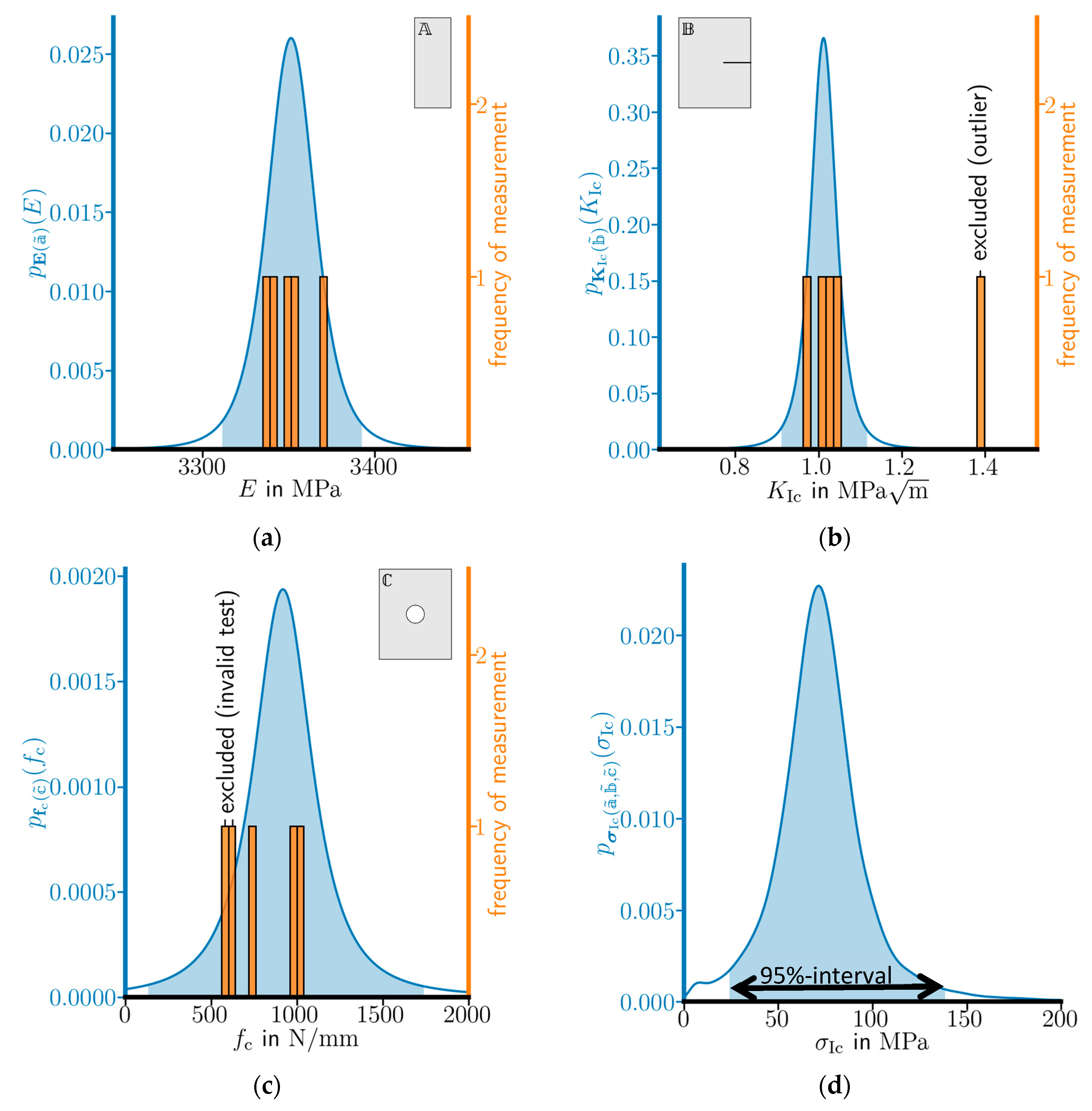
With the mean values , and listed in Table 1, the mean critical stress is computed. Furthermore, probability density functions for new realizations are plotted in Figure 8 for (a) the Young’s modulus, (b) the fracture toughness, (c) the critical load for specimen shape , and (d) the critical stress. Table 2 lists the quantiles of the probability functions. The 2.5% and 97.5% quantiles are the bounds of the 95% prediction intervals that are illustrated by a light blue filled area in Figure 8. The 95% prediction intervals in (c) and (d) are wide, because only valid tests for specimen shape are considered. The orange histograms show the measured values from Table 1, with the frequency of measurement indicating the number of samples lying in the region of the histogram bar. Since the measured Poisson’s ratio is nearly constant, we set it to a constant value .
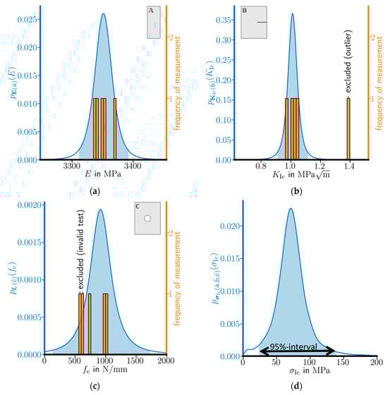
Figure 8.
Probability density functions for future realizations (blue) and histogram of measured quantities (orange) for (a) the Young’s modulus , (b) the fracture toughness , (c) the critical force in specimen shape , and (d) the predicted critical stress . The 95% prediction intervals are illustrated by the light blue filled area. The probability density distributions (a–c) are generated from random variables defined in Equations (12)–(14). The probability density distribution (d) is computed using a Monte Carlo approach.
Table 2.
Quantiles of the calibrated material parameters. The Poisson’s ratio is held constant.
3.2. Validation
For the validation, the critical position and the critical load are predicted for the specimen shapes , , and based on observations of the tests , , and . Furthermore, the validation specimen shapes are tested as , , and . Their critical loads are measured and listed in Table 1. The critical position is determined visually from the videos of the tests.
Table 3 shows the critical loads predicted by SLMM+AC and Full FEM. SLMM+AC is only evaluated with the mean material parameters. Full FEM is only applied to the potential critical positions computed by SLMM+AC, independent of whether SLMM+AC is applicable at this position or not. Full FEM uses the mean material parameters once but also uses the material parameters generated by MC for the 2.5%, 50%(i.e., median), and 97.5% quantiles. The 2.5% and 97.5% quantile build a 95% prediction interval. As can be seen in Table 3, the difference of predicted with the SLMM+AC computed using the Full FEM approach with the mean material parameters is below 12%.
Table 3.
Predicted critical loads for the specimen shapes , and . SLMM+AC and Full FEM use the mean material parameters. Full FEM quantiles are computed using a Monte Carlo method.
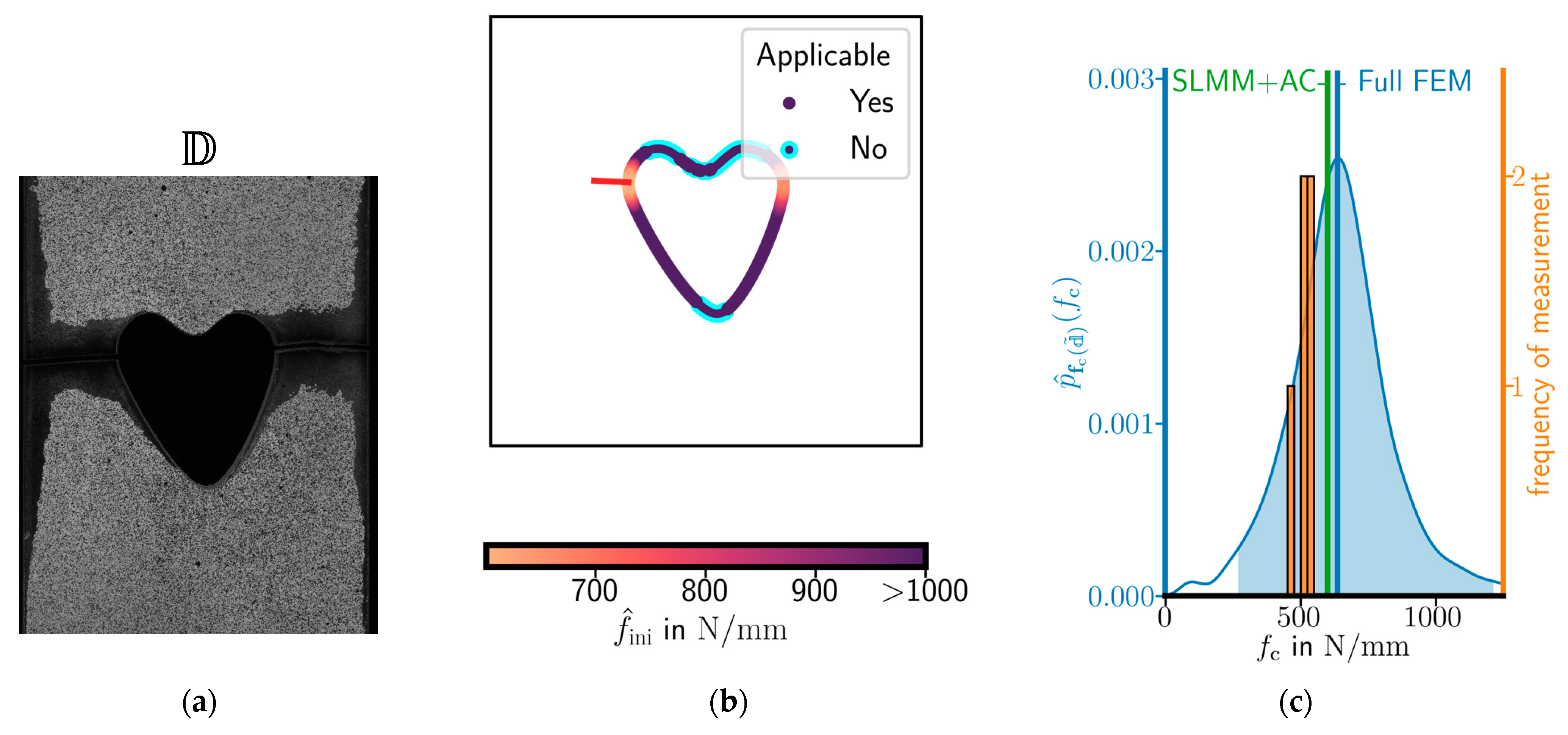
Figure 9 compares the results of the tensile test with the predictions of the heart-shaped specimen . As depicted by Figure 9a, the left crack at the heart is the position that is predicted in Figure 9b as a red line. In the test, the second crack initiated almost simultaneously with the first one. Figure 9b shows the initiation load along the cavity surface. Almost all positions are applicable and SLMM+AC can be used. The lowest initiation load is the critical load and the corresponding position is the critical position . For this position , Figure 9c plots the critical force computed by SLMM+AC, the Full FEM approach with mean material parameters, and the probability density function computed by the Full FEM approach with sampled material parameters. The light blue filled area represents the 95% prediction interval.
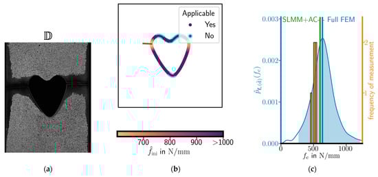
Figure 9.
Comparison of prediction and tensile tests of the heart-shaped specimen shape : (a) broken specimen, (b) predicted position of crack initiation, and (c) predicted critical loads according to SLMM+AC (mean value, green), Full FEM (mean value, blue) and experiments (orange) in terms of predicted probability density function and histogram of measured critical loads.
In the tested specimens, cracks initiated almost simultaneously on both sides. The presented approach does not consider crack initiations on both sides, which could have an influence on the critical load , as shown by Sapora et al. [13] for circular holes. They showed that the critical force deviates at most by 5.3% when considering only a one-sided crack initiation instead of crack initiation on both sides because having a second crack initiate at the same time increases local stresses in the first crack.
The measured loads for the heart-shaped specimens are between 474 and 537 N/mm with a mean value of 515.6 N/mm, which is about 14% lower than predicted by SLMM+AC, but all measured loads are inside the 95% prediction interval.
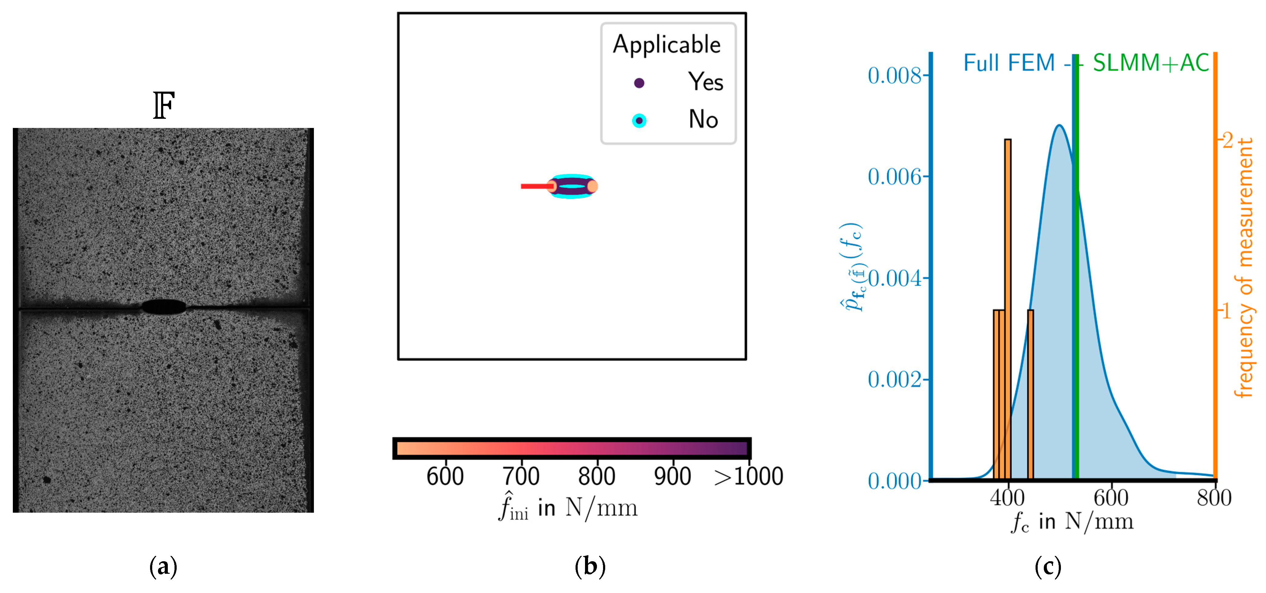
Analogously to Figure 9, Figure 10 compares the experimental results and the predictions for specimen shape . As shown by Figure 10a, the crack initiates at the right side, which is correctly predicted by SLMM+AC, as illustrated in Figure 10b. For the critical position, the critical load is predicted and plotted in Figure 10c. The measured values are between 146 and 173 N/mm and agree well with the prediction of SLMM+AC and Full FEM. The deviation of the measured mean load to the predicted SLMM+AC mean value is about 1.2%.
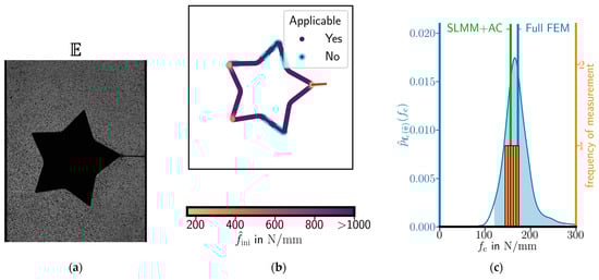
Figure 10.
Comparison of prediction and tensile tests of the specimen shape : (a) broken specimen, (b) predicted position of crack initiation, and (c) predicted critical loads according to SLMM+AC (green), Full FEM (blue), and experiments (orange) in terms of the predicted probability density function and histogram of measured critical loads.
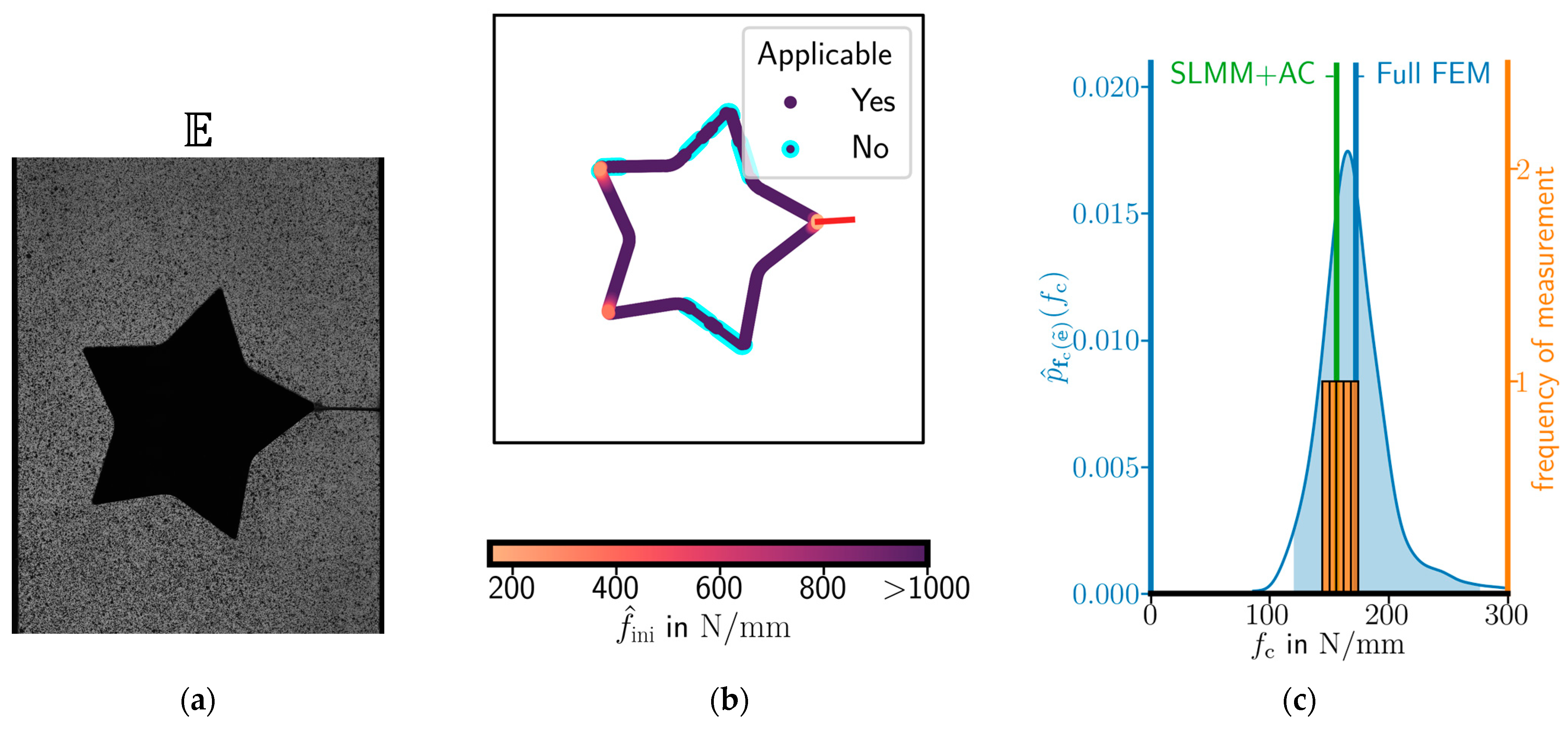
Figure 11 depicts the broken specimen and the predictions for shape . Similar to the heart-shaped specimens, in these specimens, cracks also initiated at both sides almost simultaneously as depicted by Figure 11a. Figure 11b shows that the presented approach predicts a slightly larger on the left side. Figure 11c illustrates the critical load. The measured values are between 375 and 439 N/mm. One measured value is outside of the 95% prediction interval. The deviation of the measured mean load to the critical load predicted by SLMM+AC is about 25%.
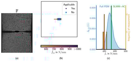
Figure 11.
Comparison of prediction and tensile tests of the specimen shape : (a) broken specimen, (b) predicted position of crack initiation, and (c) predicted critical loads according to SLMM+AC (green), Full FEM (blue), and experiments (orange) in terms of predicted probability density function and histogram of measured critical loads.
For the three validation specimen shapes , , and , the mean critical load of the experiments is 12% below, 1.2% above, and 25% below the predicted SLLM-AC values, respectively. For the specimen shapes and , the experiments lie well within the predicted interval of , whereas, for specimen shape , they are significantly lower. This can be explained by tolerances in the cavity surface, possible waviness of the cut, and pre-damaging of the PMMA sheets by the laser cutter. With the small radius of specimen shape , it makes sense that these tolerances can have a greater influence on . However, the statistical analysis used in this paper to obtain the prediction interval of does not take this geometric variation into account.
4. Conclusions
This study tested the hypothesis that the Coupled Criterion could be used to predict the crack initiation position and critical load for various specimen shapes. The incremental energy release rate was computed using either the efficient SLMM+AC approach or the computationally more expensive Full FEM approach. Probabilistic distributions were used to account for the scatter in material properties such as Young’s modulus, critical energy release rate, and critical stress. The fast SLMM+AC approach then allowed a Monte Carlo analysis to be used to obtain the prediction intervals of the critical forces for three validation tests.
The greatest variation in material properties is observed in the critical stress obtained from the specimens that contain a circular hole. This critical stress therefore also accounts for the variation in possible surface defects introduced by the laser cutter.
The previously developed efficient SLMM+AC method is additionally evaluated at critical positions along the void surface and is shown to be an efficient approximation to the Full FEM approach with a maximum deviation of 12%.
For all three validation specimens tested, the crack initiation position is correctly predicted. The critical load prediction intervals for the validation specimens are quite wide, resulting in 14 of the 15 measured maximum loads falling within the 95% prediction intervals. However, the mean predicted failure loads differ by up to 25% from the mean experimental failure loads, which is the case for the elliptical cavity (specimen shape ). For the heart-shaped and star-shaped void specimens, these deviations are much smaller at 12% and 1.2% respectively, indicating that critical stress distributions (associated with initial surface defects) may vary depending on the shape of the void cut into the PMMA sheets by the CO2 laser.
In the future, similar specimens can be used to combine crack propagation, crack arrest, and crack initiation to study the toughening effects of specific void arrangements or to introduce a soft phase in place of the voids with similar crack initiation. Based on the observations that large variations in void shape can significantly shift the levels of critical loads, special care must be taken in the selection of possible void shapes.
Author Contributions
Conceptualization, M.R. and M.P.; methodology, M.R. and M.P.; software, M.R.; validation, M.R. and C.W.; data curation, C.W. and M.R.; writing—original draft preparation, M.R. and C.W.; writing—review and editing, M.R., C.W., M.P. and C.S.; visualization, M.R. All authors have read and agreed to the published version of the manuscript.
Funding
This research received no external funding.
Data Availability Statement
The raw data supporting the conclusions of this article will be made available by the authors upon request.
Conflicts of Interest
The authors declare no conflicts of interest.
Abbreviations
The following symbols and abbreviations are used in this manuscript.
| Geometrical quantities | Acronyms | ||
| gauge length | CC | Coupled Criterion [6] | |
| clamping length | FEA (FEM) | Finite Element Analysis | |
| width | (Finite Element Method) | ||
| thickness | Full FEM | Full Finite Element Method approach [20] | |
| crack length | MA | Matched Asymptotic [11] | |
| initial crack length | MC | Monte Carlo [31] | |
| maximum applicable crack length for SLMM+AC | PMMA | Poly(methyl methacrylate) | |
| position on the notch surface | SLMM+AC | Scaling Law based Meta-Model [20] | |
| Quantities from tensile tests | SENT | Single Edge Notched Tensile [2] | |
| displacement | TCD | Theory of Critical Distances [3] | |
| force | Tensile tests () | ||
| load defined as | a specimen shape | ||
| Material quantities | an observed tensile test of the corresponding specimen shape | ||
| Young’s modulus | all observed tensile tests of the corresponding specimen shape | ||
| Poisson’s ratio | number of observed tests in | ||
| stiffness | an unobserved tensile test of the corresponding specimen shape | ||
| material toughness for mode I | Statistics | ||
| fracture energy | arbitrary quantity | ||
| critical stress | random quantity measured in the test | ||
| Irwin’s length | true mean value for tests of the specimen shape | ||
| Young’s modulus | true standard deviation for tests of the specimen shape | ||
| Computed quantities | random quantity for the mean value measured in the tests | ||
| strain energy | random quantity for the standard deviation measured in the tests | ||
| J-Integral | Cumulative probability distribution of some random quantity | ||
| (in-plane) major principal stress | Probability density function of some random quantity | ||
| incremental energy release rate | Estimator for the random quantity | ||
| Sub- and superscripts | Student’s t-distribution with degrees of freedom [30] | ||
| arbitrary quantity | Normal distribution with mean and standard deviation [31] | ||
| corresponds to the Full FEM approach | |||
| corresponds to the SLMM+AC approach | |||
| corresponds to a position where SLMM+AC is applicable | |||
| corresponds to a position where SLMM+AC is not applicable | |||
| corresponds to a FEM simulation | |||
| corresponds to a crack initiation at a specific position | |||
| critical value | |||
| lower bound for a quantity | |||
Appendix A. Incremental Energy Release Rate
The incremental energy release rate
is defined as the difference between the strain energies without a crack and with a crack at a constant displacement . The crack has a length . The difference is divided by the crack surfaces . For a linear elastic material, the strain energy
depends on the displacement and a stiffnes that decreases with a growing crack. As depicted by Figure A1, we apply a constant force instead of a constant displacement. Consequently, the displacement and the stiffness vary with the crack length. The orange curve without a crack has a higher stiffness than the green curve.
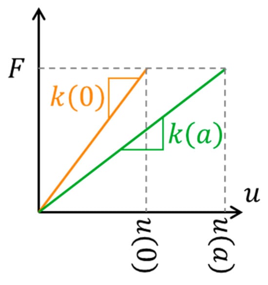
Figure A1.
Schematic force displacement curves for a constant force . The stiffness decreases with a growing crack of length .
Figure A1.
Schematic force displacement curves for a constant force . The stiffness decreases with a growing crack of length .
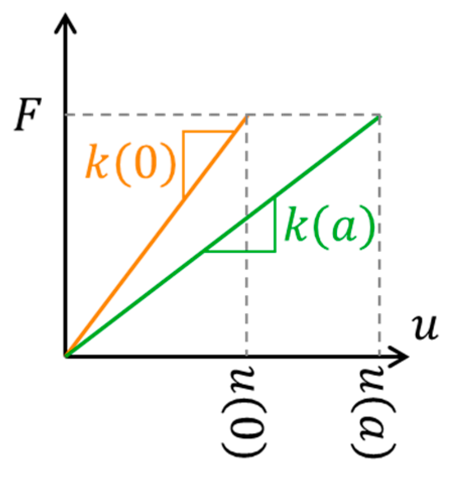
The stiffness
is the ratio between the applied force and the measured displacement . With , Equations (A2) and (A3), we can rewrite Equation (A1) to the following:
References
- Christensen, R.M. The Theory of Materials Failure, 1st ed.; Oxford University Press: Oxford, UK, 2013; ISBN 978-0-19-966211-1. [Google Scholar]
- Anderson, T.L. Fracture Mechanics: Fundamentals and Applications; CRC Press: Boca Raton, FL, USA, 1991; ISBN 978-0-8493-4277-6. [Google Scholar]
- Taylor, D. Predicting the Fracture Strength of Ceramic Materials Using the Theory of Critical Distances. Eng. Fract. Mech. 2004, 71, 2407–2416. [Google Scholar] [CrossRef]
- Taylor, D.; Cornetti, P.; Pugno, N. The Fracture Mechanics of Finite Crack Extension. Eng. Fract. Mech. 2005, 72, 1021–1038. [Google Scholar] [CrossRef]
- Cornetti, P.; Pugno, N.; Carpinteri, A.; Taylor, D. Finite Fracture Mechanics: A Coupled Stress and Energy Failure Criterion. Eng. Fract. Mech. 2006, 73, 2021–2033. [Google Scholar] [CrossRef]
- Leguillon, D. Strength or Toughness? A Criterion for Crack Onset at a Notch. Eur. J. Mech. A/Solids 2002, 21, 61–72. [Google Scholar] [CrossRef]
- Doitrand, A.; Duminy, T.; Girard, H.; Chen, X. A Review of the Coupled Criterion. J. Theor. Comput. Appl. Mech. 2024. [Google Scholar] [CrossRef]
- Leguillon, D.; Yosibash, Z. Crack Onset at a V-Notch. Influence of the Notch Tip Radius. Int. J. Fract. 2003, 122, 1–21. [Google Scholar] [CrossRef]
- Yosibash, Z.; Priel, E.; Leguillon, D. A Failure Criterion for Brittle Elastic Materials under Mixed-Mode Loading. Int. J. Fract. 2006, 141, 291–312. [Google Scholar] [CrossRef]
- Leguillon, D.; Quesada, D.; Putot, C.; Martin, E. Prediction of Crack Initiation at Blunt Notches and Cavities—Size Effects. Eng. Fract. Mech. 2007, 74, 2420–2436. [Google Scholar] [CrossRef]
- Doitrand, A.; Martin, E.; Leguillon, D. Numerical Implementation of the Coupled Criterion: Matched Asymptotic and Full Finite Element Approaches. Finite Elem. Anal. Des. 2020, 168, 103344. [Google Scholar] [CrossRef]
- Yosibash, Z.; Mendelovich, V.; Gilad, I.; Bussiba, A. Can the Finite Fracture Mechanics Coupled Criterion Be Applied to V-Notch Tips of a Quasi-Brittle Steel Alloy? Eng. Fract. Mech. 2022, 269, 108513. [Google Scholar] [CrossRef]
- Sapora, A.; Torabi, A.R.; Etesam, S.; Cornetti, P. Finite Fracture Mechanics Crack Initiation from a Circular Hole. Fatigue Fract. Eng. Mater. Struct. 2018, 41, 1627–1636. [Google Scholar] [CrossRef]
- Doitrand, A.; Sapora, A. Nonlinear Implementation of Finite Fracture Mechanics: A Case Study on Notched Brazilian Disk Samples. Int. J. Non-Linear Mech. 2020, 119, 103245. [Google Scholar] [CrossRef]
- Li, X.; Xie, Z.; Zhao, W.; Zhang, Y.; Gong, Y.; Hu, N. Failure Prediction of Irregular Arranged Multi-Bolt Composite Repair Based on Finite Fracture Mechanics Model. Eng. Fract. Mech. 2021, 242, 107456. [Google Scholar] [CrossRef]
- Ferrian, F.; Cornetti, P.; Marsavina, L.; Sapora, A. Finite Fracture Mechanics and Cohesive Crack Model: Size Effects through a Unified Formulation. Frat. Integrità Strutt. 2022, 16, 496–509. [Google Scholar] [CrossRef]
- Romani, R.; Bornert, M.; Leguillon, D.; Le Roy, R.; Sab, K. Detection of Crack Onset in Double Cleavage Drilled Specimens of Plaster under Compression by Digital Image Correlation—Theoretical Predictions Based on a Coupled Criterion. Eur. J. Mech. A/Solids 2015, 51, 172–182. [Google Scholar] [CrossRef]
- Li, J.; Leguillon, D. Finite Element Implementation of the Coupled Criterion for Numerical Simulations of Crack Initiation and Propagation in Brittle Materials. Theor. Appl. Fract. Mech. 2018, 93, 105–115. [Google Scholar] [CrossRef]
- Molnár, G.; Doitrand, A.; Estevez, R.; Gravouil, A. Toughness or Strength? Regularization in Phase-Field Fracture Explained by the Coupled Criterion. Theor. Appl. Fract. Mech. 2020, 109, 102736. [Google Scholar] [CrossRef]
- Rettl, M.; Pletz, M.; Schuecker, C. Efficient Prediction of Crack Initiation from Arbitrary 2D Notches. Theor. Appl. Fract. Mech. 2022, 119, 103376. [Google Scholar] [CrossRef]
- Bažant, Z.P. Size Effect in Blunt Fracture: Concrete, Rock, Metal. J. Eng. Mech. 1984, 110, 518–535. [Google Scholar] [CrossRef]
- DIN EN ISO 527-2:2012-06; Kunststoffe—Bestimmung Der Zugeigenschaften—Teil_2: Prüfbedingungen Für Form- Und Extrusionsmassen (ISO_527-2:2012); Deutsche Fassung EN_ISO_527-2:2012. Beuth Verlag GmbH: Berlin, Germany, 2012. [CrossRef]
- Kobayashi, T.; Shockey, D.A. Fracture Surface Topography Analysis (FRASTA)—Development, Accomplishments, and Future Applications. Eng. Fract. Mech. 2010, 77, 2370–2384. [Google Scholar] [CrossRef]
- Bura, E.; Seweryn, A. The Fracture Behaviour of Notched PMMA Specimens under Simple Loading Conditions—Tension and Torsion Experimental Tests. Eng. Fail. Anal. 2023, 148, 107199. [Google Scholar] [CrossRef]
- Barsoum, R.S. On the Use of Isoparametric Finite Elements in Linear Fracture Mechanics. Numer. Meth Eng. 1976, 10, 25–37. [Google Scholar] [CrossRef]
- Leguillon, D.; Martin, E.; Sevecek, O.; Bermejo, R. What Is the Tensile Strength of a Ceramic to Be Used in Numerical Models for Predicting Crack Initiation? Int. J. Fract. 2018, 212, 89–103. [Google Scholar] [CrossRef]
- Grubbs, F.E. Sample Criteria for Testing Outlying Observations. Ann. Math. Statist. 1950, 21, 27–58. [Google Scholar] [CrossRef]
- Rice, J.R. A Path Independent Integral and the Approximate Analysis of Strain Concentration by Notches and Cracks. J. Appl. Mech. 1968, 35, 379–386. [Google Scholar] [CrossRef]
- Geisser, S. Predictive Inference: An Introduction; Springer: Boston, MA, USA, 1993; ISBN 978-0-412-03471-8. [Google Scholar]
- Student The Probable Error of a Mean. Biometrika 1908, 6, 1. [CrossRef]
- Meeker, W.Q.; Hahn, G.J.; Escobar, L.A. Statistical Intervals: A Guide for Practitioners and Researchers, 2nd ed.; Wiley series in probability and statistics; Wiley: Hoboken, NJ, USA, 2017; ISBN 978-0-471-68717-7. [Google Scholar]
- Scott, D.W. Multivariate Density Estimation: Theory, Practice, and Visualization, 1st ed.; Wiley Series in Probability and Statistics; Wiley: Hoboken, NJ, USA, 1992; ISBN 978-0-471-54770-9. [Google Scholar]
- Atkins, A.G.; Lee, C.S.; Caddell, R.M. Time-Temperature Dependent Fracture Toughness of PMMA: Part 1. J. Mater. Sci. 1975, 10, 1381–1393. [Google Scholar] [CrossRef]
- Atkins, A.G.; Lee, C.S.; Caddell, R.M. Time-Temperature Dependent Fracture Toughness of PMMA: Part 2. J. Mater. Sci. 1975, 10, 1394–1404. [Google Scholar] [CrossRef]


Disclaimer/Publisher’s Note: The statements, opinions and data contained in all publications are solely those of the individual author(s) and contributor(s) and not of MDPI and/or the editor(s). MDPI and/or the editor(s) disclaim responsibility for any injury to people or property resulting from any ideas, methods, instructions or products referred to in the content. |
© 2025 by the authors. Licensee MDPI, Basel, Switzerland. This article is an open access article distributed under the terms and conditions of the Creative Commons Attribution (CC BY) license (https://creativecommons.org/licenses/by/4.0/).