Abstract
The cryptocurrency market has grown significantly, and this quick growth has given rise to scams. It is necessary to put fraud detection mechanisms in place. The challenge of inadequate labeling is addressed in this work, which is a barrier to the training of high-performance supervised classifiers. It aims to lessen the necessity for laborious and time-consuming manual labeling. Some unlabeled data points have labels that are more pertinent and informative for the supervised model to learn from. The viability of utilizing unsupervised anomaly detection algorithms and active learning strategies to build an iterative process of acquiring labeled transactions in a cold start scenario, where there are no initial-labeled transactions, is being investigated. Investigating anomaly detection capabilities for a subset of data that maximizes supervised models’ learning potential is the goal. The anomaly detection algorithms under performed, according to the results. The findings underscore the need that anomaly detection algorithms be reserved for situations involving cold starts. As a result, using active learning techniques would produce better outcomes and supervised machine learning model performance.
1. Introduction
The technological evolution experienced in recent years, with the emergence of new computing technologies, makes Machine Learning (ML) today different from ML of the past. Because of its capacity to extract patterns from data that would help organizations identify profitable business opportunities or avoid risks, this kind of technology is now used in almost every kind of business.
In parallel with technological development, there is a growing concern about detecting fraudulent behavior in financial transactions. Therefore, despite all the effort and investment put into fraud prevention, there is still a need for efficient Fraud Detection (FD) mechanisms [1,2,3,4]. Traditional financial systems have extensively used these approaches to detect unusual fraudulent behaviors.
The market for cryptocurrencies has grown exponentially in recent years, leading to its widespread acceptance as a form of digital currency. Nevertheless, the surge in popularity has also drawn a plethora of fraudulent activities, including insider trading, phishing, Ponzi schemes, and money laundering. As a result, there is an urgent need to protect the integrity of the cryptocurrency market, which presents a significant opportunity to investigate FD mechanisms in this area.
As a multi-asset digital money platform that provides financial services to a global market and enables users to transact in digital currencies, Uphold serves as the study’s focus. As a result, this work will offer FD mechanisms that will enable Uphold to spot new fraudulent activity in bitcoin transactions.
1.1. Problem Definition
Three main problems justify this work. The first problem concerns the need for labeled data within the FD domain, rendering it impractical to train highly effective supervised ML models using historical information. Specifically, within the financial domain, companies often lack labeled datasets, meaning that they do not possess transaction-level labels indicating whether each transaction is licit or illicit.
Furthermore, the arduous and time-consuming nature of labeling an enormous volume of transactions makes it an impractical undertaking for organizations. This happens due to the complex nature of fraudulent behavior. As a result, the second problem becomes intricately linked to the first.
Given the time and budget constraints companies face when reviewing transactions, there is an urgent requirement to develop mechanisms that empower analysts to concentrate their investigative efforts on transactions that are most likely to involve fraud. By doing so, valuable resources and time can be saved by bypassing the examination of low-information data instances unlikely to provide significant insights.
Finally, Uphold faces an ongoing challenge due to the ever-evolving nature of criminal behavior. In today’s world, criminals constantly seek innovative methods to commit fraudulent crimes. This issue is particularly prominent in the cryptocurrency markets, where criminals exploit the vulnerabilities of cryptocurrencies.
The lack of regulation and the anonymity of cryptocurrencies makes them attractive for fraudulent activities. As a company operating in this space, Uphold is susceptible to the risks associated with illicit activities. Such risks can have severe consequences, compromising the trust of its users and exposing the company to compliance with laws and regulations. Therefore, adopting practical approaches to detect these new fraudulent behaviors is crucial.
1.2. Objectives
Thus, the primary motivation for this project will be to extract the best of both unsupervised and supervised worlds and efficiently detect fraudulent patterns in cryptocurrency transactions by identifying data points that do not conform to the standard transaction patterns and may indicate fraudulent behavior. This would help gain insights that can be applied in the Uphold platform to catch illicit transactions.
Assuming a cold start scenario, it is intended with this work to assess the feasibility of using Anomaly Detection (AD) algorithms [1,5] and Active Learning (AL) techniques [6] to uncover fraudulent patterns in cryptocurrency transactions [7].
Thus, the main objective is to gain insights into the practical relevance of using AD approaches with AL, to gather relevant labeled transactions iteratively. The purpose of gathering these labels is to train and improve a supervised classifier’s performance to achieve optimal performance using a minimal number of labels. Therefore, the feasibility of using these methods to select a subset of labeled data that maximizes the supervised model’s performance.
The primary objective of this research is to tackle fraud in the domain of cryptocurrencies using AD and AL algorithms. This includes addressing problems such as the scarcity of labels for training supervised ML models and the dynamic nature of fraudulent patterns.
1.3. Methodologies
For the project’s development, we used DSR (Design Science Research) [8], which provides a set of metrics ideas for the research process. The DSR approach is a research methodology that seeks to generate and evaluate solutions to practical problems by utilizing and implementing theoretical concepts and techniques.
1.4. Document Structure
This article is divided into five sections: Section 1 presents the background, motivation, and objectives. Section 2 deals with the tools and materials used in the work. It includes explanations of the tools employed, the dataset used, and the corresponding characteristics and distributions, and it also presents a detailed description of the experiments carried out. It covers the pre-processing procedures and provides explanations of the experimental setup, including details of the implementation of each algorithm and the parameters chosen. In Section 3, the results of the study are presented. Section 4 discusses the results. We end with the conclusions of this project, the difficulties and a point regarding potential future work, highlighting areas for further research and development, all presented in Section 5.
2. Materials and Methods
With the rapid advancement of technology, the problem of financial fraud has gained greater urgency. The widespread adoption of digital transactions across numerous industries has unfortunately given rise to a corresponding increase in electronic criminal activities [9].
Cryptocurrency markets are especially vulnerable to different types of scams and fraudulent activities. This is due to the lack of regulation stemming from the decentralized nature of the market [10] and the anonymity that virtual currencies provide to criminals and their transactions [2], as users can own multiple addresses and can only be identified by them [11].
Thus, developing effective strategies for identifying and preventing fraudulent behavior in transactional data is crucial for companies such as Uphold [5].
There are many alternative ways to fight financial fraud. However, because of the dynamic and complex nature of fraudulent behavior, the development of effective FD mechanisms, leveraging available data, will always be necessary as it is impossible to completely prevent all types of fraud [12]. In other words, criminal behavior continues to evolve as criminals find new ways to carry out their fraudulent activities. Given this, it is crucial to continuously improve these methods to effectively detect and address new patterns of fraudulent behavior [4].
ML algorithms play a crucial role in identifying fraudulent patterns in transactional data due to their ability to perform tasks involving high-level pattern recognition [13].
In simpler terms, the primary aim is to efficiently identify a subset of data for annotation that optimizes the model’s learning capacity [14]. Moreover, commonly used metrics for evaluation include learning curves.
This section presents the materials and tools employed in this research study. The section encompasses a detailed overview of the libraries utilized to implement the techniques evaluated in this study and the dataset and its exploratory data analysis.
It is important to note that the dataset selection, pre-processing, and exploratory data analysis were conducted collaboratively as a team at Uphold. Additionally, another student on the team worked on a fraud-related use case. Given that the supervisors were the same, there was some overlap in the materials used and the exploration of those materials.
The programming language chosen for the development of this project and its auxiliary scripts is Python, a powerful, high-level language well-suited for ML projects. It offers excellent flexibility, a wide range of resources, and comprehensive documentation. Additionally, its simplicity and ease of use can significantly enhance developer productivity, allowing them to focus on solving problems rather than struggling with the intricacies of the language itself. Its open-source nature and large developer community make it an ideal choice for this project.
The programming environment used in this work was Jupyter Notebook. Jupyter Notebook is an interactive computing environment that facilitates creating and disseminating documents incorporating live code, equations, visualizations, and explanatory text. It boasts a web-based interface that supports the generation and execution of code cells, thereby simplifying the process of experimentation, iteration, and collaboration on data analysis and ML endeavors.
Python has a diverse set of tools and libraries specifically tailored for ML. This project utilized the following libraries: Scikit-learn, XGBoost, and Pyod. For auxiliary tasks, the following libraries were necessary: NumPy, Pandas, Scipy, and Matplotlib.
This work uses the Elliptic Dataset, the world’s largest publicly available cryptocurrency transaction dataset. This dataset was created to facilitate the creation of innovative methods for detecting fraudulent activity in cryptocurrency transactions.
This dataset was selected for the following reasons:
- The fact that this is a representative dataset of cryptocurrency transactional data makes it valuable for exploring the feasibility of using AD and AL algorithms to detect fraudulent patterns.
- The existence of labeled samples (licit and illicit transactions) allows an easy simulation of the AL process by linking the class label to the queried transaction.
- Previous exploration of unsupervised AD techniques combined with AL strategies has been performed on this specific dataset [14].
- The dataset pertains to the Bitcoin transactions network, which is of great interest because Bitcoin is the most well-known and secure cryptocurrency.
Before presenting the specifics of the Elliptic Dataset, it is essential to understand how Bitcoin transactions work.
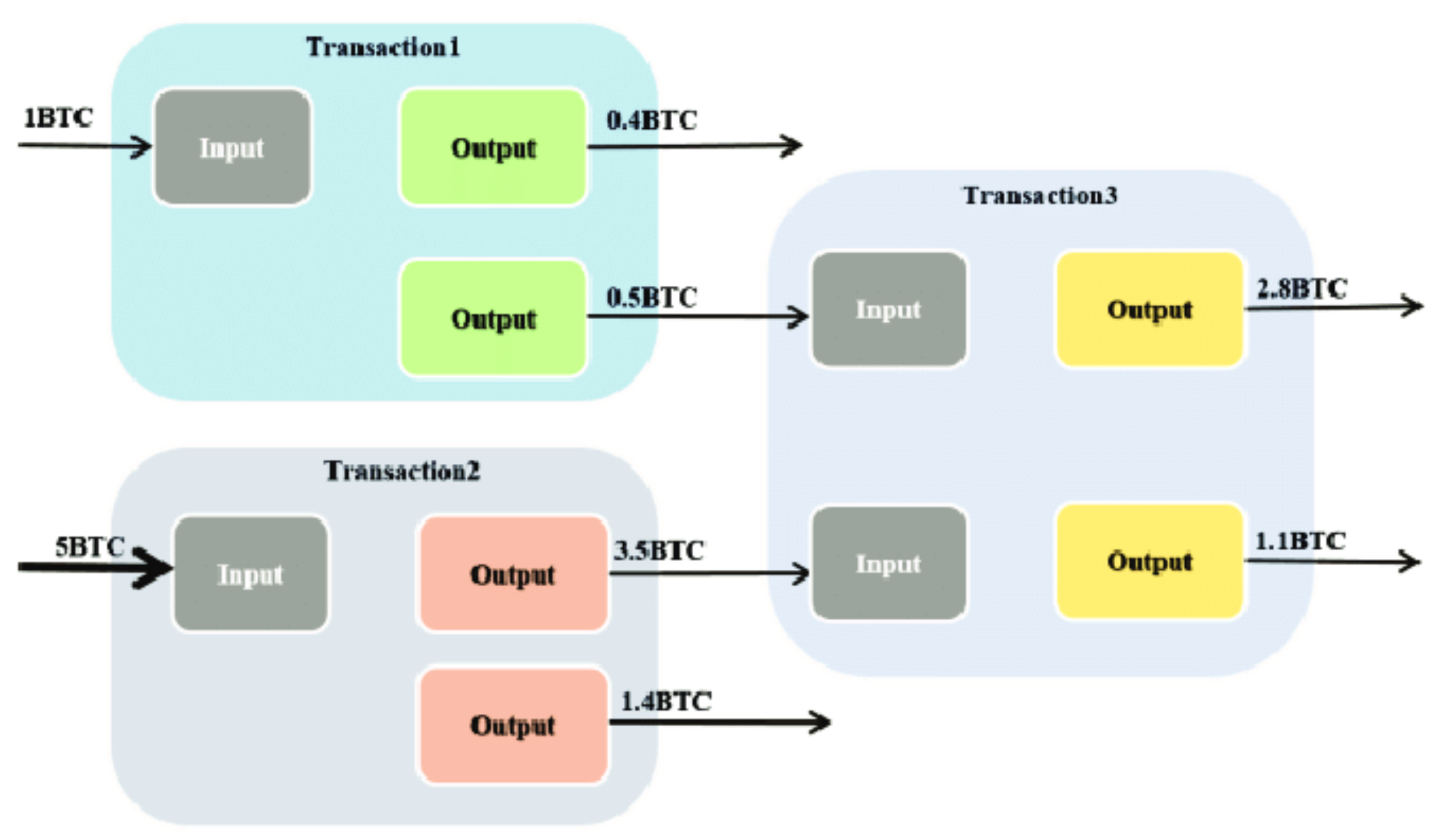
Bitcoin transactions operate on a protocol known as Unspent Transaction Output (UTXO), which enforces specific rules [15]. When a user (A) intends to send a payment to another user (B), user A needs to reference the prior transaction where they received the funds; this reference to the preceding transaction is called the transaction input. The transfer of funds to user B is the transaction output. It is worth noting that a transaction can involve multiple inputs and outputs, allowing for more complex scenarios.
Figure 1 illustrates the Bitcoin UTXO transaction model.
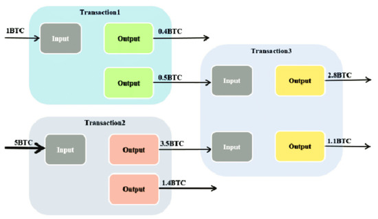
Figure 1.
Bitcoin UTXO transaction model [15].
The Elliptic Dataset contains over 200,000 transactions from the Bitcoin blockchain and maps them to real entities in either licit, illicit, or unknown categories. Labels include “licit” for transactions made by regulated exchanges, licit services, miners, etc., and “illicit” for dark markets, scams, malware, terrorism organizations, Ponzi schemes, etc.
The dataset includes 49 transaction graphs sampled from the Bitcoin blockchain at different points in time. Each node in the graph represents a transaction with 166 anonymised features and is labeled as “licit”, “illicit”, or “unknown”. The graph consists of 203,769 nodes and 234,355 edges (regarding the flow of Bitcoin transactions).
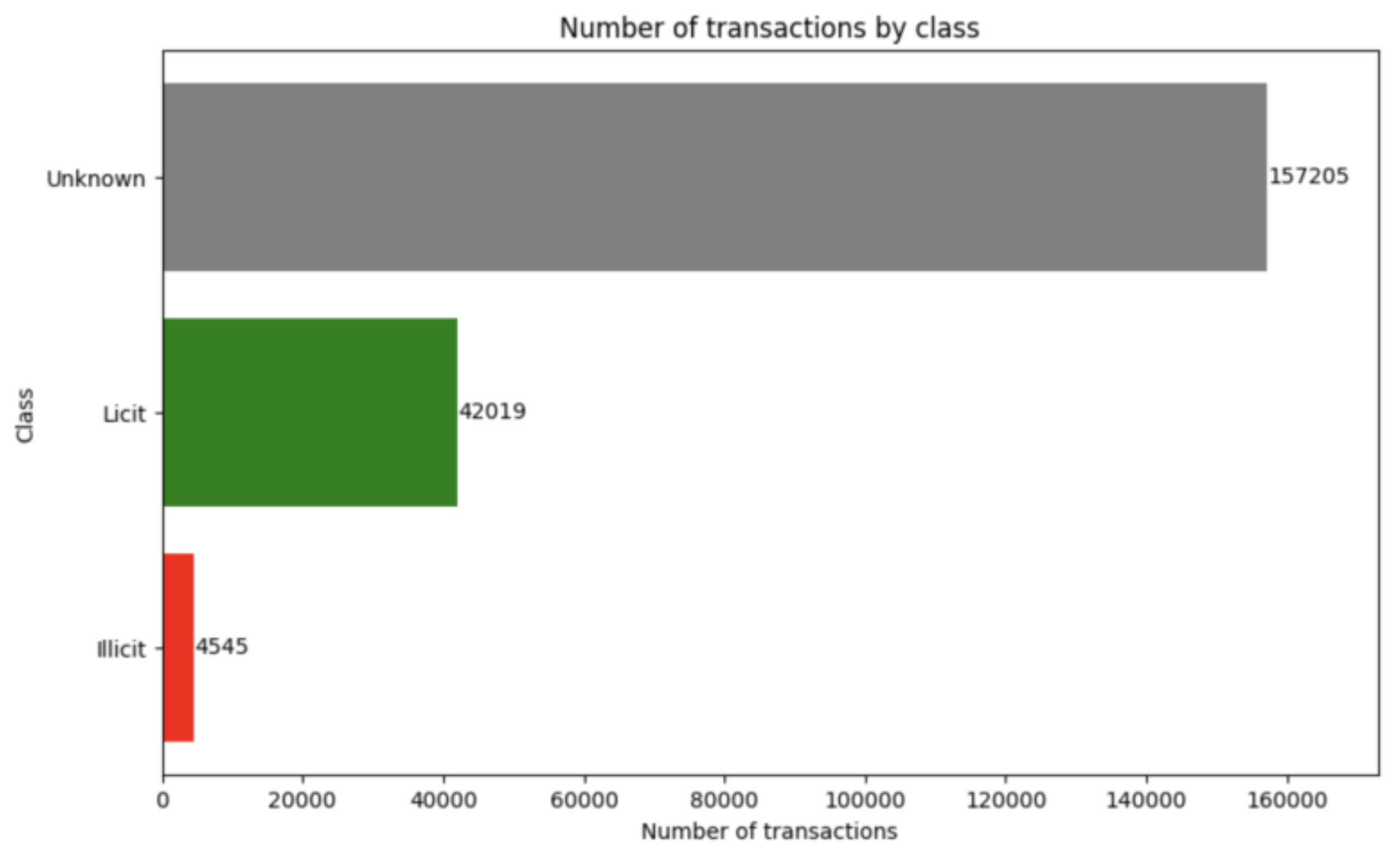
A total of 4545 Bitcoin transactions are labeled illicit, corresponding to approximately 2% of the total transaction nodes. Moreover, 42,019 transactions are labeled as licit ones, which corresponds to 21% of the graph nodes. The remaining 157,205 transactions (77% of the total transactions) are not labeled regarding the licit vs. illicit, thereby being represented as “unknown” transactions.
The transaction address, time step, and class label are the only known information in the anonymised data. The time step measures when a transaction was broadcast to the network and ranges from 1 to 49, with a two-week interval between each.
The first 94 features pertain to local information about the transaction, such as the time step, number of inputs/outputs, transaction fee, and aggregated information like average BTC received/spent. The remaining 72 features are aggregated using one-hop backward/forward information from the center node and include neighboring transactions’ maximum, minimum, standard deviation, and correlation coefficients.
2.1. Analyze AD in Cryptocurrency Transactions with AL
This section presents an overview of the proposed solutions and the experimental setup. It will provide a detailed description of the experiments designed to address the objectives and challenges described in the introduction to this document. In doing so, it aims to understand the methodologies used clearly.
2.1.1. Data Structure
The main dataset consisted of three distinct datasets, each containing specific information about the transactions and the flow of transactions. These datasets include data about transaction classes, transaction features, and transaction edges:
- The dataset about the classes comprises two distinct features. The initial feature, , is a categorical variable denoting unique identifiers for each transaction. The subsequent feature is the categorical target label, encompassing three possible values: , , or . Based on the dataset characteristics, it helps classify transactions as fraudulent.
- The second dataset, focusing on the edges, captures essential information about the connections or links between transactions. It provides valuable insights into the relationships or associations among distinct transactions. As such, this dataset is characterized by two categorical features. The first feature denotes the source , while the second feature corresponds to the target .
- The third and final dataset consists of the transaction ID and a comprehensive collection of other relevant features. This dataset encompasses a wide array of transaction-related information, enabling a meticulous analysis and profound understanding of the attributes and properties associated with each transaction. Thus, the dataset is composed of a total of 168 features. These features include the , , 94 , and 72 .
2.1.2. Exploratory Data Analysis
The key findings derived from a comprehensive exploratory data analysis are delved into. Undertaking this crucial step provides a better understanding of the label targets and the underlying dataset before applying ML algorithms. The primary focus of the exploratory data analysis was to gain a deep understanding of the label targets. Through careful examination, essential information about these targets, such as their distributions and potential class imbalances, has been uncovered.
The plot in Figure 2 is a bar plot that showcases the cumulative count of transactions across the class labels.

Figure 2.
Number of transactions by class.
The visualization indicates that the dataset predominantly comprises transactions labeled as “unknown”, which account for a substantial total of 157,205 transactions. Moreover, the plot effectively demonstrates a significant class imbalance, as the number of recorded illicit transactions is 4545.
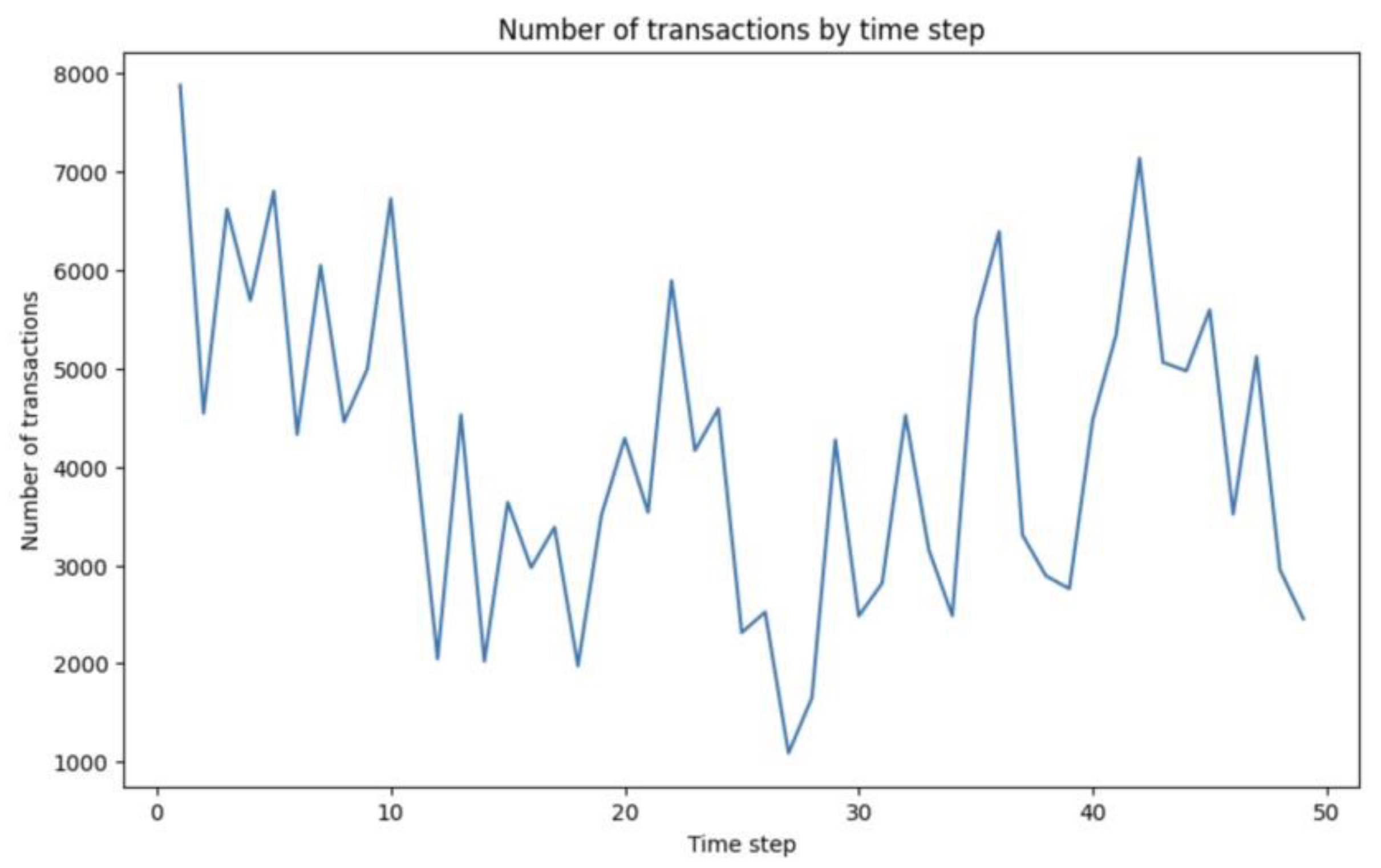
Figure 3 shows a line plot that portrays the cumulative transactions count across various time steps.
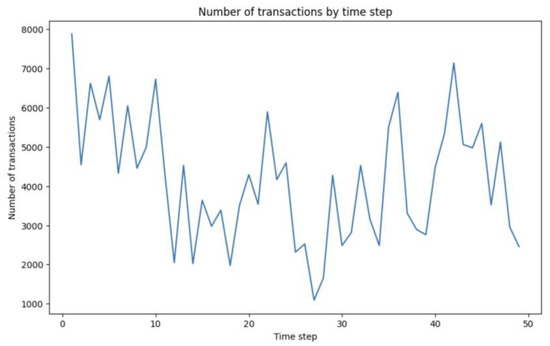
Figure 3.
Number of transactions by time step.
The plot reveals significant variations in the total number of transactions observed over time steps. Notably, specific time steps exhibit several transactions approximately seven to eight times higher than others, indicating a substantial disparity. This considerable fluctuation underscores the dynamic nature of transaction activity over the recorded period.
The stacked bar plot presented in Figure 4 complements the visualization depicted in Figure 2 by illustrating the distribution of class labels across different time steps.
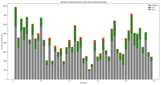
Figure 4.
Number of transactions for each class in each time step.
By analyzing this plot, it becomes evident that the overall pattern observed in the dataset remains consistent across all time steps, thereby offering significant insights. The dataset shows a greater frequency of unknown transactions than labeled ones, where illicit activities constitute only a tiny portion.
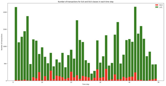
Figure 5.
Number of transactions for licit and illicit classes in each time step.
This particular plot enables a more comprehensive examination of the proportion of illicit versus licit transactions at each time step. Consistent with the findings of Weber et al. (2019), it can be concluded that a notable decline in the number of illicit transactions occurred between time steps 43 and 46, attributed to an abrupt cessation of the dark market.
Lastly, Figure 6 employs t-distributed Stochastic Neighbor Embedding (t-SNE), a widely used dimensionality reduction technique for visualizing high-dimensional data in a lower-dimensional space, more specifically, in this case, in a two-dimensional representation.
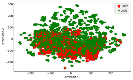
Figure 6.
t-SNE representation of the true labels.
The plot illustrates that fraudulent behavior lacks a discernible pattern, as the instances are scattered across the plot without any distinct clustering, overlapping with typical transaction behavior. This observation supports the notion that fraudsters often mimic normal transaction behavior, making their activities challenging to identify based on visual patterns alone.
2.2. Data Pre-Processing
The primary aim of data pre-processing is to improve the correctness of the dataset and enhance its efficacy during the modeling stages.
The main changes made to the dataset are described as follows:
- Convert the categorical labels to integers: the original target labels in the dataset were categorical, represented as ’1’, ’2’, and ’unknown’. In order to enhance comprehensibility, the target labels were transformed from categorical values into integers. Specifically, ’2’ was converted to 0 to indicate licit transactions, ’1’ was changed to 1 to represent illicit transactions, and ’unknown’ was transformed to −1.
- Consider only the labeled samples: this step involved filtering the dataset to focus solely on labeled samples. As stated, the dataset comprised three primary target categories: 0 (licit transactions), 1 (illicit transactions), and −1 (unknown transactions). However, to test the supervised algorithms and simulate the AL setup effectively, only the labeled samples (licit and illicit) were used here. This approach enabled this work to associate the original labels with the transactions chosen for querying. Consequently, it eliminated the need for a human analyst to review all selected transactions.
- Rename the transaction features: in order to improve the comprehensibility of the feature datasets, more representative names were assigned for the transaction features. For example, it was assigned column names such as , or . Note that there are 93 local features and 72 aggregated features. This renaming step was essential because the original dataset lacked descriptive names for all the transaction features. By undertaking this process, the aim was to make the dataset more interpretable and provide a clearer understanding of the underlying information each feature represents.
- Merge classes and features datasets: this step involved merging the feature and class datasets, thereby combining the label and feature information for each transaction. The classes and feature information for each transaction were stored in separate datasets. To perform this merge operation, the transaction IDs from both datasets were mapped together.
After the data preparation steps, the refined dataset consisted of 46,564 labeled transactions.
2.3. Experimental Setup
To maintain consistency with the work of [14] on the same dataset, it follows a similar approach in dividing the data into sequential train and test datasets for all experiments. The training dataset encompasses 29,894 transactions for all experiments, comprising all labeled samples until the 34th time step. In comparison, the testing dataset consists of 16,670 transactions, including labeled samples from the 35th time step onwards. It is important to note that the train set comprises 10% of illicit cases.
To guarantee reproducibility and consistency in the experiments, a systematic approach was implemented using a predetermined seed value (e.g., 8,347,658) at the start of the code execution. This seed value was utilized to initialize the random number generator, which determined the sequence of random operations throughout the experiments. By following this methodology, it was possible to ensure that the experiments could be reliably replicated, enabling consistent evaluation and comparison of the models.
To establish a supervised baseline for benchmarking various AL setups, the initial step of the experiments involved training a set of supervised classifiers on the 166 features of the train set and then evaluating them on the test set. This involves training the supervised classifiers on the available training set (29,894 transactions).
Three supervised algorithms were tested: RF, XGBoost, and LR. It is used in the scikit-learn implementation of RF, the scikit-learn implementation of LR, and the Python implementation of XGBoost.
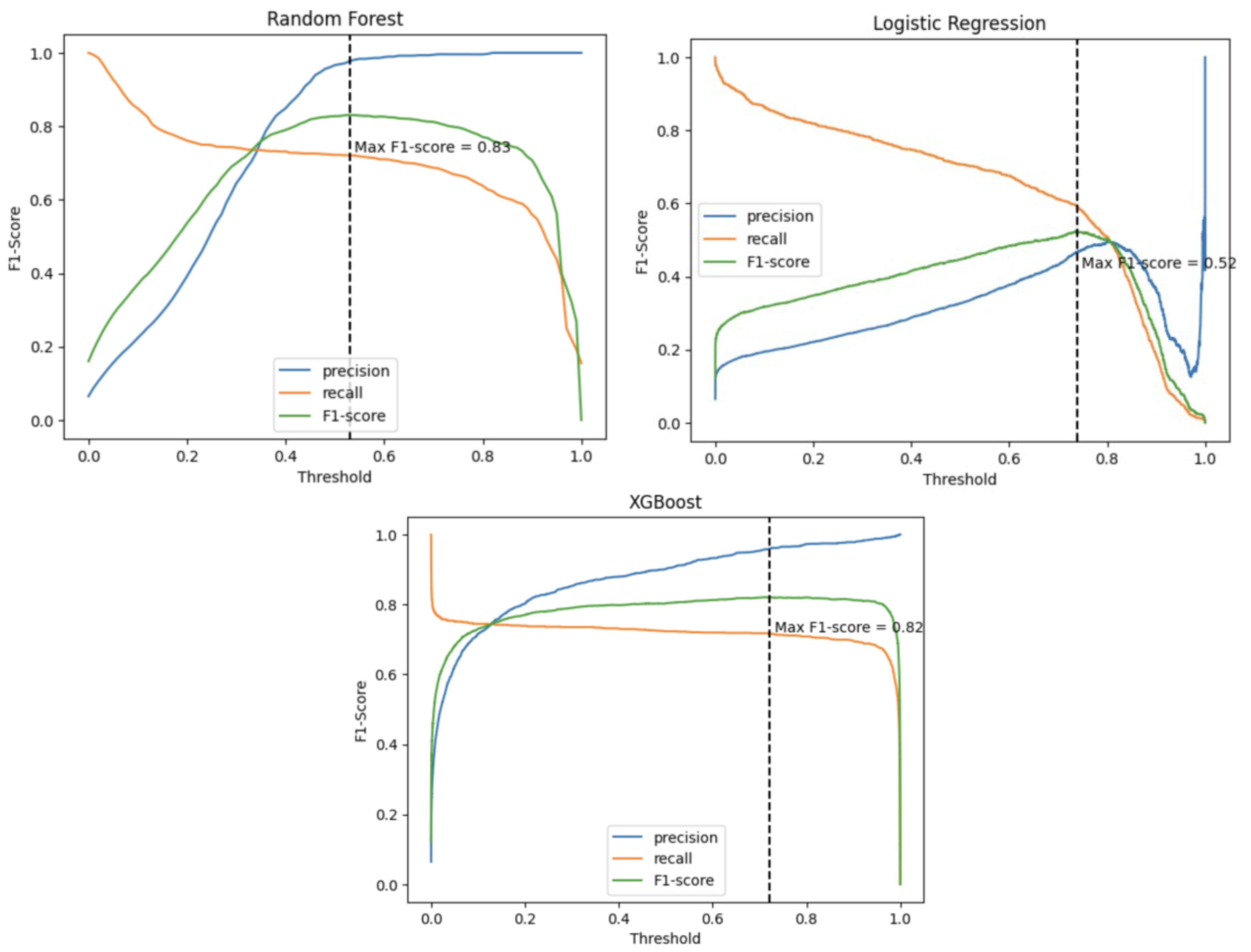
For evaluating the performance, the maximum F1-score is reported. This score is determined by finding the threshold that maximizes the F1-score based on the predicted probabilities from each supervised classifier. Furthermore, the precision and recall values are also reported at this specific threshold, comprehensively evaluating the classifier’s performance. Note that all these metrics were reported using the scikit-learn library.
In addition to the maximum F1-score, the performance of the supervised classifiers over time is measured by reporting the F1-score per time step on the test set. This enables tracking the classifiers’ effectiveness and identifying any variations in performance throughout the evaluation. By analyzing the F1-score over time, it is possible to gain insights into the classifiers’ consistency and adaptability in handling the test data.
Lastly, to introduce additional randomness and variability, a unique random state was implemented for each of the supervised classifiers tested. The random state was generated using a random integer function. Subsequently, this newly generated random state value was passed as a parameter (“”) during the model initialization phase.
Active Learning
In the AL experiments, there were six different query strategies. Among these, three were unsupervised: Elliptic Envelope, IF, and LOF. The remaining three strategies were supervised: EMC, QBC, and Uncertainty Sampling.
All experiments use a batch size of 50 transactions sampled at each iteration of the AL process until a total of 3000 labeled transactions (60 iterations) are collected. This means that only the top 50 most informative/relevant transactions will be selected for labeling at each iteration. This corresponds to executing each AL setup until the labeled pool comprises approximately 10% of the total transactions initially available in the training set.
It is important to note that at the beginning of the execution of each AL setup, the training set is divided into two pools: labeled and unlabeled. Initially, the labeled pool contains no labeled transactions (cold start scenario), but as the AL process progresses, it gradually accumulates labeled transactions through iterative increments of 50 transactions. The transactions chosen for labeling during each iteration are subsequently removed from the unlabeled pool for further iterations.
As supervised algorithms, the three supervised classifiers evaluated in the supervised baseline were utilized: RF, LR, and XGBoost. The performance of each AL setup was assessed through the maximum F1-score at each labeled pool size.
It means that a supervised classifier will be trained on the available labeled pool at each iteration and assessed its performance on the test set. The performance of each supervised classifier is compared against its respective supervised baseline, described in the Supervised Baseline chapter. Additionally, the respective learning curves of each AL setup execution will be provided, showing the evolution of the F1-score through the different labeled pool sizes.
The AL experiments were divided into two main steps/scenarios:
- Scenario 1—Unsupervised AL policies: in this scenario, the focus is on utilizing only unsupervised query strategies. The aim is to assess the effectiveness of unsupervised AD algorithms as AL policies to iteratively (at each iteration) query the most relevant fraud-related patterns within the unlabeled pool (the most anomalous transactions). Instead of transitioning to a supervised AL policy, this approach solely relies on an unsupervised AD algorithm used as an AL policy throughout the entire AL process. To provide an additional baseline for comparison, there will also be evaluated setups where a Random Sampling algorithm is used instead of an unsupervised learner.
- Scenario 2—Combine unsupervised and supervised AL policies: this scenario aims to determine the optimal point to switch from an unsupervised to a supervised AL policy. In this scenario, the AL setup will start by querying the most anomalous transactions until a certain threshold occurs. To define this optimal cut-off point, the number of iterations (AL loop executions) is used as a basis. Specifically, once a predefined number of iterations is completed, the setup will automatically transition from an unsupervised learner to a supervised learner.
Given these previous considerations, Figure 7 depicts the operational mechanisms of the AL experiments.

Figure 7.
Simplified structure of an active learning setup.
This visualization represents a simplified structure of the execution of each AL setup where the condition “iteration <= threshold” determines whether an unsupervised or supervised AL policy is employed. When the condition is proper, it indicates that the current iteration of the AL process is still below the predetermined threshold (cut-off point), indicating the execution of an unsupervised AL policy. Conversely, when the condition is false, the current iteration has surpassed the threshold, triggering the execution of a supervised AL policy.
Each AL setup executed in the experiments comprises a combination of one unsupervised policy, one supervised policy (depending on the scenario being executed), and one supervised classifier. It is worth noting that each loop execution corresponds to a new iteration of the AL process, and each AL setup is executed for 60 iterations. At each iteration of the AL process, 50 transactions will be queried for labeling.
It is possible to observe that all the AL setups will start with an unsupervised AL policy, since the condition “iteration <= threshold” will never be false at the first iteration. Starting the AL process with an unsupervised AD algorithm is imperative, since there are no labeled transactions at the beginning.
A supervised AL policy is implemented as soon as the threshold criterion is met. Exceptionally, scenario 1 will be executed when the predefined total number of AL iterations per setup (60 iterations) is equal to the predefined threshold. Therefore, the supervised AL policy will never be executed in that case since the condition “iteration <= threshold” will always be valid for every iteration in the AL process.
The supervised policies are trained on the available labeled pool to identify the most informative instances within the unlabeled data. On the other hand, the unsupervised policies are trained on the unlabeled pool, and the anomaly scores are also computed on the same unlabeled pool.
Each AL setup will be run once, except for the baseline setups that use the Random Sampling algorithm. Since more variability is expected with a completely random algorithm, each setup that uses the Random Sampling algorithm was executed five times. In this case, the median F1-score was recorded at each labeled pool size.
Below is a comprehensive overview of the models and parameters utilized for the AL experiments:
- A summary of the model parameters used for each unsupervised AL policy (IF, LOF, and Elliptic Envelope) implemented using the PyOD library.
- For Uncertainty Sampling, the same supervised classifier is employed to evaluate the performance of the AL setup on the test. For example, if an RF classifier was used to evaluate the AL setup’s performance, RF was also used for Uncertainty Sampling.
- Regarding QBC, it was used the scikit-learn implementation of RF with n_estimators = 100, max_depth = 3, and class_weight = ‘balanced’. This approach measures the disagreement between the predicted probabilities of 100 DTs for each unlabeled instance.
- Considering EMC, a custom binary LR model trained with gradient descent was built.
Further, a unique random state is generated at each iteration to introduce additional randomness and variability. This random state was obtained using a random integer function. During the model initialization phase, the newly generated random state value was passed as a parameter (“random_state = random_state*”).
The following points describe the main approaches that were tested:
- Feature subset selection for training AD algorithms: this exploratory approach involved training AD algorithms using different subsets of features from the dataset. Determining the most significant features makes it possible to train the anomaly detectors more effectively and enhance their prediction accuracy.
- Examining bitcoin transaction network properties: the second approach involved considering the inherent characteristics of the bitcoin transaction network. This policy incorporated the anomaly scores calculated for the transactions within the unlabeled pool and the transactions associated with previously identified illicit activities (illicit transactions already discovered in previous iterations). As a result, only transactions with higher anomaly scores, which were also connected to other known illicit transactions in the network, were selected for labeling.
- Consider the unknown transactions: approximately 77% of the dataset consists of unknown transactions. The idea was to train the anomaly detector in each iteration using all transactions up to the 34th time step. This includes considering the transactions labeled as unknown and the remaining transactions in the unlabeled pool. The anomalous score would then be computed solely for the unlabeled pool.
3. Results
This section thoroughly examines the outcomes attained through experimentation with the methodologies elucidated in the preceding chapters.
3.1. Supervised Baseline
The research findings suggest that the supervised baseline models outperformed the study [14] regarding F1-score performance. This improvement can be credited to the study’s emphasis on determining the ideal thresholds for maximizing the F1-score instead of relying on the default threshold offered by the scikit-learn library. By explicitly analyzing the thresholds that produced the highest F1-scores, this approach significantly enhanced the supervised model’s performance within the scope of this investigation.
Figure 8 presents the evolution of precision, recall, and F1-score across different thresholds.
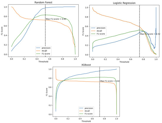
Figure 8.
Supervised baseline metrics by threshold.
After locating the peak F1-score, the optimal threshold is established, followed by extracting the precision and recall values associated with this particular threshold. A summary of the results for each model can be found in Table 1.

Table 1.
Supervised baseline results.
The results from the experiments indicate that both the RF and XGBoost models exhibit commendable performance in terms of F1-score, precision, and recall. These models demonstrate good overall performance with F1-scores of 0.83 and 0.82, respectively. Furthermore, both models achieve high precision scores, with RF at 0.98 and XGBoost at 0.96, suggesting that most optimistic predictions are accurate.
On the other hand, the LR model performs comparatively worse, as evidenced by its lower F1-score of 0.52. This suggests poorer overall performance compared to RF and XGBoost models. The LR model also exhibits a lower precision score of 0.47, indicating higher FP predictions. This model showed a trade-off between identifying more TP instances and generating more FP, with a higher recall but a lower precision rate.
Figure 9 displays a t-SNE projection that visualizes the distribution of the actual labels within the test set, providing a realistic depiction of their spatial arrangement.
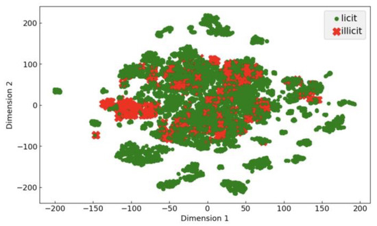
Figure 9.
t-SNE projection on the test set, colored by the true labels.
Based on Figure 9, it becomes evident that a considerable number of illicit transactions are concentrated on the left side of the plot. Furthermore, the remaining illicit transactions are distributed across the entire plot.
Figure 10 presents a t-SNE projection that provides a visual representation of how the predicted labels are distributed within the test set for each of the supervised classifiers evaluated in the supervised baseline.
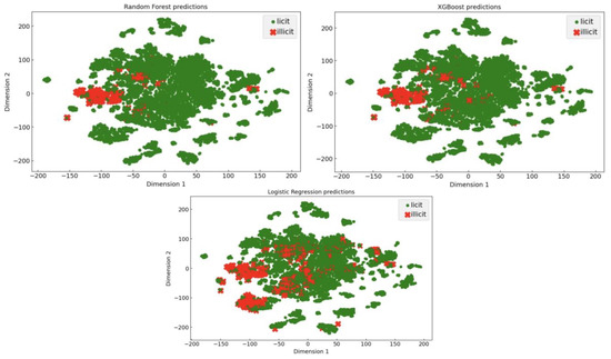
Figure 10.
t-SNE projection on the test set, colored by the predicted labels of the supervised classifiers.
Based on the analysis of these plots, it becomes evident that the RF and XGBoost models exhibit remarkable similarities in their performance. Notably, they effectively identify the significant portion of illicit transactions prominently clustered on the left side of the plot. These visualizations align with previous considerations, indicating that most positive predictions these models make are accurate, resulting in high precision values.
However, these methods still need to capture many illicit transactions (recall is substantially lower). In contrast, the LR model displays inadequate results, indicating its poor performance in correctly identifying the positive/fraudulent instances.
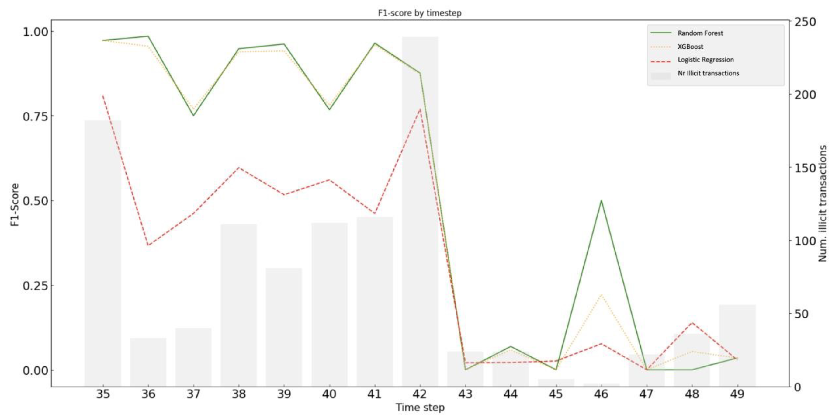
Figure 11 depicts the F1-score performance of each supervised classifier across the different time steps.
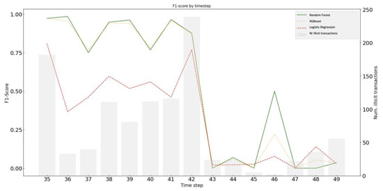
Figure 11.
F1-score by time step, for each supervised classifier.
Based on the findings presented in Figure 11, it becomes evident that the performance of each supervised classifier is significantly impacted by the abrupt cessation of the dark market, which occurred after time step 43.
3.2. Active Learning
The outcomes from these experiments will be consolidated in a table, including both the unsupervised and supervised AL policies employed.
For consistency with the work of [14], the unsupervised AL policies will be referred to as AL warm-up learners, while the supervised ones will be referred to as AL hot learners. The table will also provide information about the classifier that will be trained on the available labeled data for each setup.
The results will be presented for labeled pools of 200, 500, 1000, 1500, and 3000 transactions. Additionally, each classifier used in the AL setups will be compared against its baseline, i.e., the performance they achieve when trained on the entire train set.
3.2.1. Scenario 1—Unsupervised Active Learning Policies
First, the results of scenario 1 will be presented, thereby not switching from an unsupervised policy to a more sophisticated supervised policy at any point in the AL process. The results are shown in Table 2, Table 3 and Table 4, regarding each one of the supervised classifiers: RF, XGBoost, and LR, respectively.
Table 2 shows the performance of the AL setups executed for the RF classifier.

Table 2.
Results of the active learning setups for Random Forest.
Table 2.
Results of the active learning setups for Random Forest.
| Classifier | Warm-Up Learner | Hot Learner | Labeled Pool Size | Baseline F1-Score | ||||
|---|---|---|---|---|---|---|---|---|
| 200 | 500 | 1000 | 1500 | 3000 | ||||
| (0.7%) | (1.7%) | (3.3%) | (5%) | (10%) | ||||
| RF | LOF | - | 0.76 | 0.77 | 0.77 | 0.78 | 0.79 | 0.83 |
| Elliptic Envelope | - | 0.49 | 0.53 | 0.57 | 0.55 | 0.54 | ||
| IF | - | - | - | - | - | 0.04 | ||
| Random Sampling | - | 0.77 | 0.77 | 0.79 | 0.79 | 0.8 | ||
Table 3 shows the performance of the AL setups executed for the XGBoost classifier.

Table 3.
Results of the active learning setups for Extreme Gradient Boosting.
Table 3.
Results of the active learning setups for Extreme Gradient Boosting.
| Classifier | Warm-Up Learner | Hot Learner | Labeled Pool Size | Baseline F1-Score | ||||
|---|---|---|---|---|---|---|---|---|
| 200 | 500 | 1000 | 1500 | 3000 | ||||
| (0.7%) | (1.7%) | (3.3%) | (5%) | (10%) | ||||
| XGBoost | LOF | - | 0.75 | 0.75 | 0.76 | 0.76 | 0.78 | 0.82 |
| Elliptic Envelope | - | 0.62 | 0.68 | 0.7 | 0.68 | 0.65 | ||
| IF | - | - | - | - | - | 0.17 | ||
| Random Sampling | - | 0.75 | 0.75 | 0.78 | 0.79 | 0.8 | ||
Table 4 shows the performance of the AL setups executed for the LR classifier.

Table 4.
Results of the active learning setups for Logistic Regression.
Table 4.
Results of the active learning setups for Logistic Regression.
| Classifier | Warm-Up Learner | Hot Learner | Labeled Pool Size | Baseline F1-Score | ||||
|---|---|---|---|---|---|---|---|---|
| 200 | 500 | 1000 | 1500 | 3000 | ||||
| (0.7%) | (1.7%) | (3.3%) | (5%) | (10%) | ||||
| LR | LOF | - | 0.43 | 0.28 | 0.29 | 0.34 | 0.36 | 0.52 |
| Elliptic Envelope | - | 0.19 | 0.25 | 0.29 | 0.3 | 0.31 | ||
| IF | - | - | - | - | - | 0.14 | ||
| Random Sampling | - | 0.41 | 0.41 | 0.44 | 0.47 | 0.45 | ||
Based on the available information, it can be observed from the tables that, regardless of the classifiers used, employing a Random Sampling algorithm as a warm-up learner yields comparable or even superior performance compared to more sophisticated AL setups that utilize unsupervised AD algorithms.
These results are unexpected since it would be anticipated that AD algorithms, despite their susceptibility to FP, would identify more meaningful fraud-related patterns than a completely random algorithm, thereby exerting a more significant influence on the overall performance of the supervised classifiers. However, what was observed is precisely the opposite. It is possible to understand that the transaction queries by the Random Sampling algorithm provoke a faster improvement in the overall performance of the three supervised ML models.
It is also important to note that still, none of the setups tested were able to reach the supervised baseline of each supervised classifier, thereby suggesting, as it was stated in the literature, that a possible transition to a supervised learner at some point in the AL process would be potentially beneficial.
On the other hand, LOF was the AD algorithm that managed to identify more meaningful transactions, but it still failed to outperform the performance achieved by the Random Sampling algorithm.
It is important to note that the overall poor performance of AD algorithms can be attributed to their limitations in effectively detecting illicit transactions based on the specific set of features that were used. The anomalies flagged by these algorithms are often FP and are not indicative of fraudulent cryptocurrency activity. In simple words, transactions identified as deviating significantly from the expected behavior or normal patterns, as determined by the AD algorithms, do not necessarily turn out to be fraudulent. This could potentially be justified, due to the intrinsic characteristics of the cryptocurrency market.
One possible explanation that could justify the comparable results obtained from using the Random Sampling algorithm is that the classifier would start approaching relatively good performance when the labeled pool includes a sufficient number of illicit transactions. Given that the training set consists of approximately 10% illicit cases, Random Sampling can quickly reach the desired number of illicit transactions. Since there are 50 transactions sampled at each iteration, on average, there will be five illicit transactions sampled per iteration with Random Sampling.
To account for this, the same setups were tested with a more realistic class imbalance. Therefore, a random under-sampling technique was employed on the minority class to achieve an illicit rate of 1%.
A comprehensive overview of the outcomes obtained from this experiment can be found in Table 5. Note that the baseline score of each supervised classifier was also updated based on the new illicit rate of 1%.

Table 5.
Results of active learning setups at 1% illicit rate.
The results presented in Table 5 focus solely on LOF and Random Sampling, as neither the Elliptic Envelope nor the IF algorithms could detect illicit transactions within the unlabeled pool throughout the AL process.
For a specific set of features, even at lower illicit rates, it can be observed that Random Sampling still surprisingly outperforms AD algorithms. These findings underscore even more the subpar performance of AD algorithms in detecting illicit transactions and the limited feasibility of utilizing them to uncover meaningful fraudulent patterns within the unlabeled pool that can be used to improve the overall performance of the supervised classifiers. For this specific set of features, using a Random Sampling algorithm would cause a more significant impact on the performance of the supervised classifiers compared to the use of AD algorithms.
Therefore, it has been demonstrated that using a Random Sampling algorithm offers a more efficient resolution to the challenges posed by cold start scenarios when contrasted with AD algorithms. These further highlight previous considerations, as the AD algorithms proved ineffective in accurately identifying fraudulent transactions based on this specific set of features. Even the most anomalous transactional patterns did not correspond to fraudulent activity.
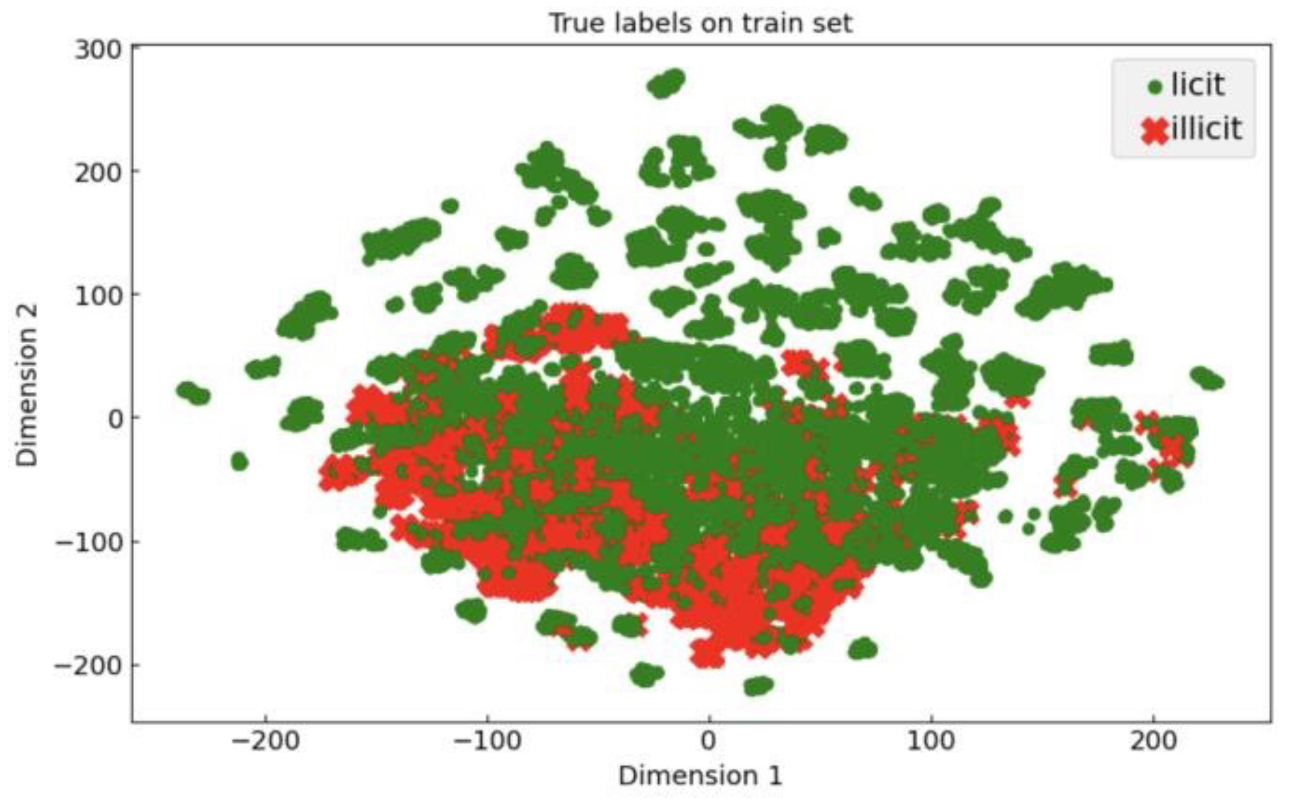
Overall, neither of the AD algorithms find relevant fraudulent transactions in the unlabeled pool that can benefit the overall model’s performance, which can be explained and visualized in Figure 12.

Figure 12.
t-SNE projection on the train set, colored by the true labels.
From Figure 12, it becomes evident that the illicit transactions within the training set are not merely outliers or deviant patterns for this set of features. This poses a significant challenge for AD algorithms in identifying fraudulent transactions, as illicit transactions exhibit similar patterns to regular transactions.
3.2.2. Scenario 2—Combining Unsupervised and Supervised Active Learning Policies
For the results of scenario 2, only the results obtained for the 30th and 1st iteration cut-off points are used, as they are representative of the overall behavior of the AL setups across all thresholds.
Firstly, the obtained results from employing unsupervised AL policies up to the 30th iteration (until the labeled pool contains 1500 transactions) are presented. The results are illustrated in Table 6, Table 7 and Table 8, regarding each one of the supervised classifiers: RF, XGBoost, and LR.

Table 6.
Results of the active learning setups for random forest (cut-off—30th iteration).

Table 7.
Results of the active learning setups for Extreme Gradient Boosting (cut-off—30th iteration)).

Table 8.
Results of the active learning setups for Logistic Regression (cut-off—30th iteration).
Table 6 depicts the results from the AL setups executed for the RF classifier.
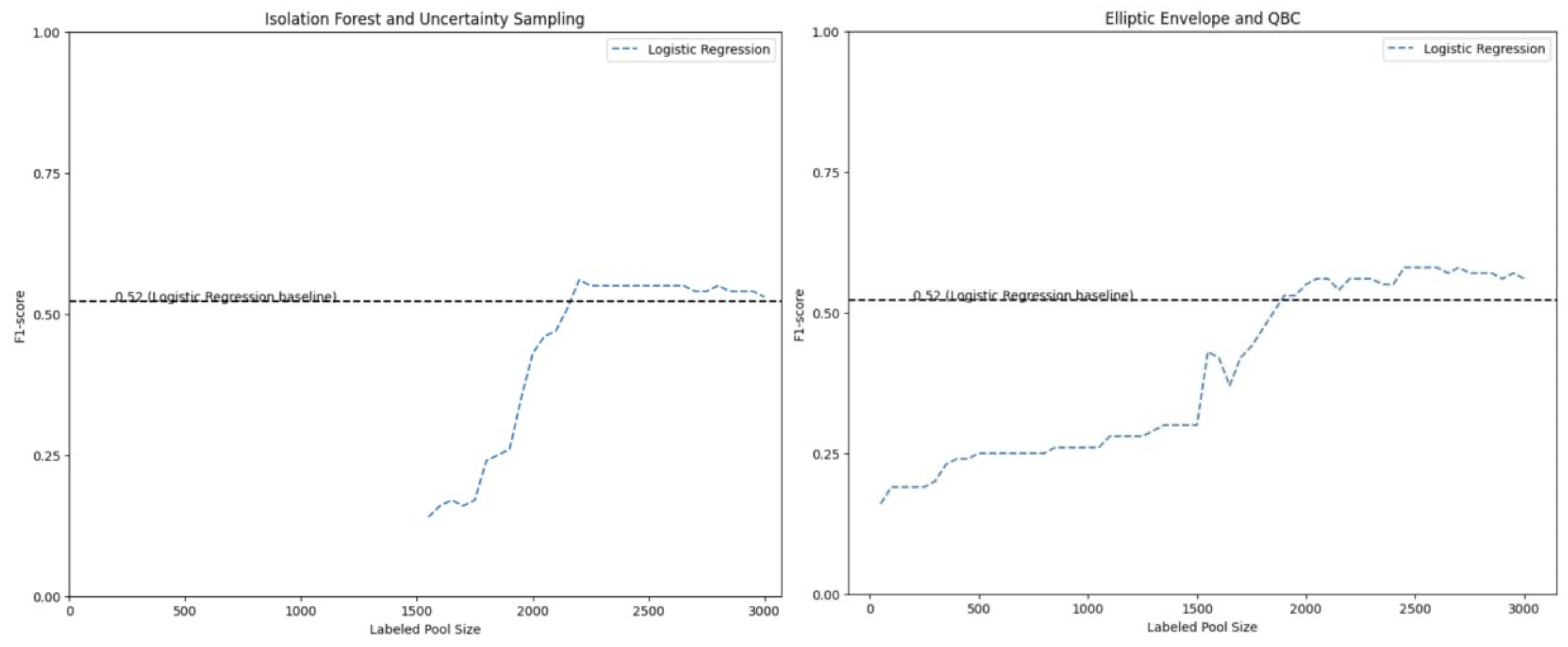
The results presented in Table 6 demonstrate a significant improvement in the performance of the RF classifier when transitioning to a supervised AL policy. By comparing the classifier’s performance with 1500 labeled transactions to that with 3000 labeled transactions, it becomes evident how quickly the F1-score improves.
In most cases, the classifier achieved a near-optimal solution, matching the baseline F1-score, with as few as 3000 labeled transactions. This accounts for only 10% of the original labels in the training set. These findings highlight the superior performance of supervised policies compared to unsupervised ones. Moreover, these results suggest that lowering the cut-off point to switch from unsupervised policies earlier in the AL process will likely benefit the classifier’s overall performance. This adjustment would lead to a potentially faster increase in its performance.
These findings also underscore the limitations of AD algorithms in identifying relevant illicit transactions within the unlabeled pool, particularly when contrasted with policies that rely on supervised classifiers. As a result, these findings suggest that there is no need to prolong the use of unsupervised AD policies throughout the AL setup.
Furthermore, the optimal performance of these supervised AL policies can be inferred by examining the results obtained from setups utilizing IF as a warm-up learner. In this context, IF detects an illicit transaction only at the 31st iteration. However, even after applying the supervised AL policies to the remaining 29 iterations, it is still possible to attain the supervised baseline for the setup that employs IF and Uncertainty Sampling.
These findings emphasize the effectiveness of supervised AL policies and the potential for optimizing the classifier’s performance by adjusting the threshold for transitioning from unsupervised policies earlier in the AL process.
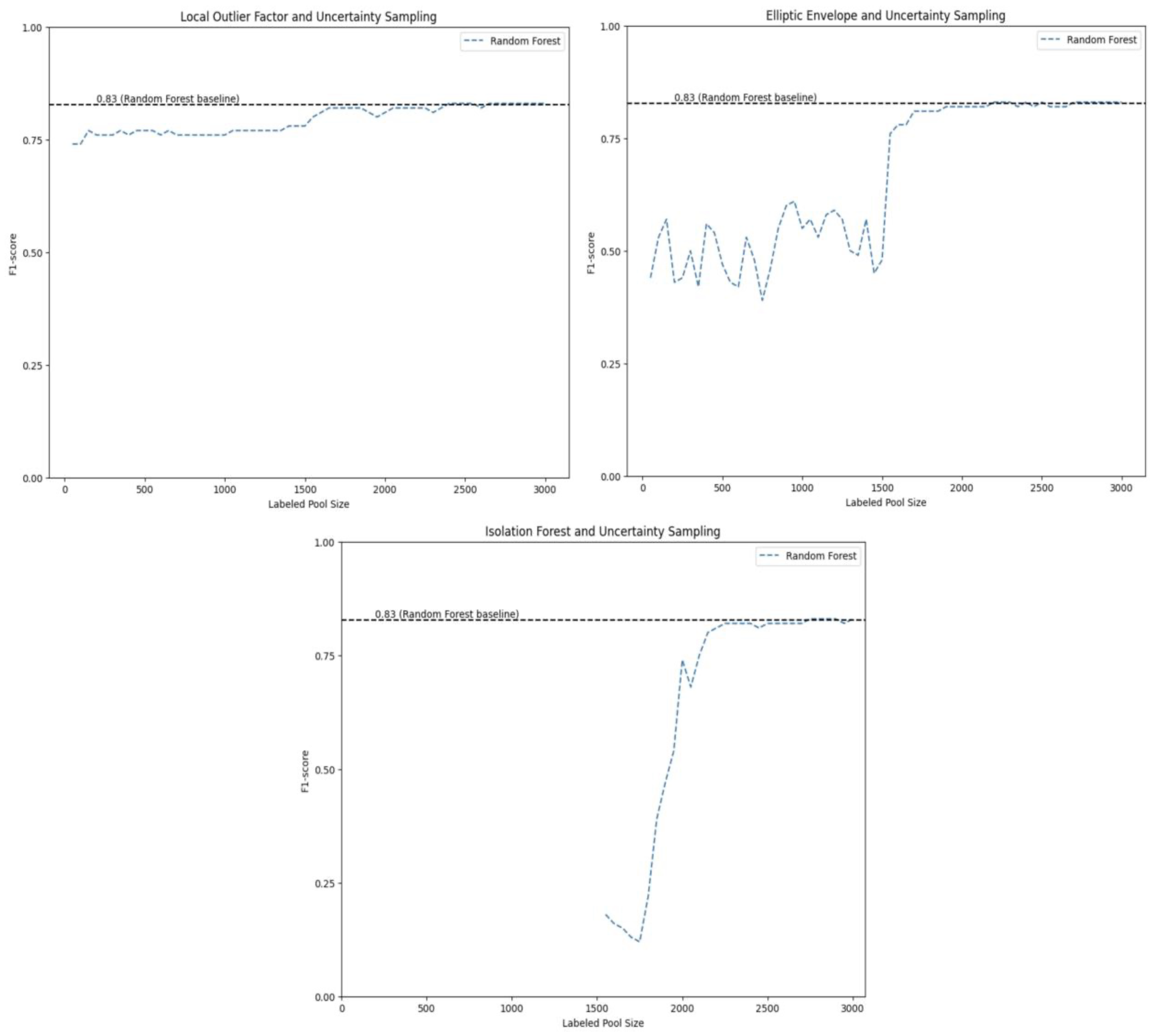
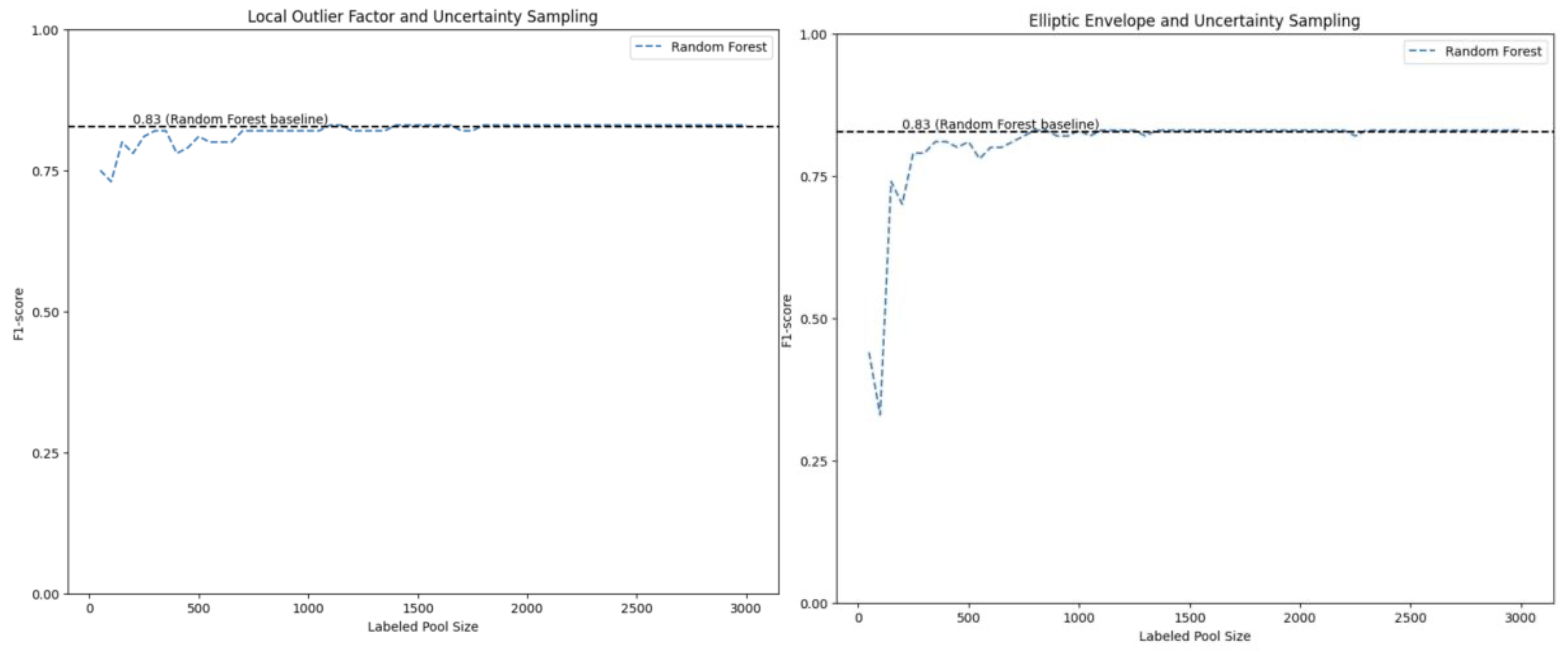
The best-performing setups utilize LOF and Uncertainty Sampling, as well as Elliptic Envelope and Uncertainty Sampling or IF and Uncertainty Sampling. Figure 13 illustrates the progression of the F1-score across various labeled pool sizes, showcasing the evolution of the results.
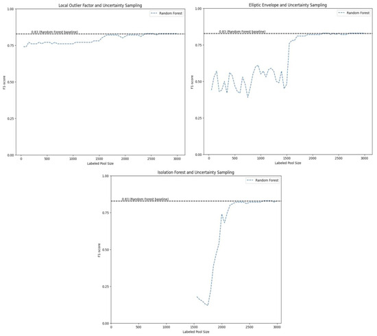
Figure 13.
Learning curves for the best performing Random Forest setups (cut-off—30th iteration).
By analyzing Figure 13, it becomes evident that the RF classifier exhibits accelerated improvement when an AL policy, such as Uncertainty Sampling, is applied. These plots visually confirm the conclusion that once the cut-off point is reached and a supervised AL policy is implemented, there is a substantial enhancement in the model’s performance. Remarkably, it is possible to observe that the baseline F1-score can be achieved with as few as 2000 labels, indicating the efficiency of these approaches.
Table 8 illustrates the results from the AL setups executed for the XGBoost classifier.
Based on the findings presented in Table 7, it is evident that the XGBoost classifier exhibits a similar trend to the RF classifier. When a supervised AL policy is implemented in the 31st iteration, the performance of the XGBoost classifier shows a rapid enhancement, with the F1-score baseline being achieved using just 3000 labels.
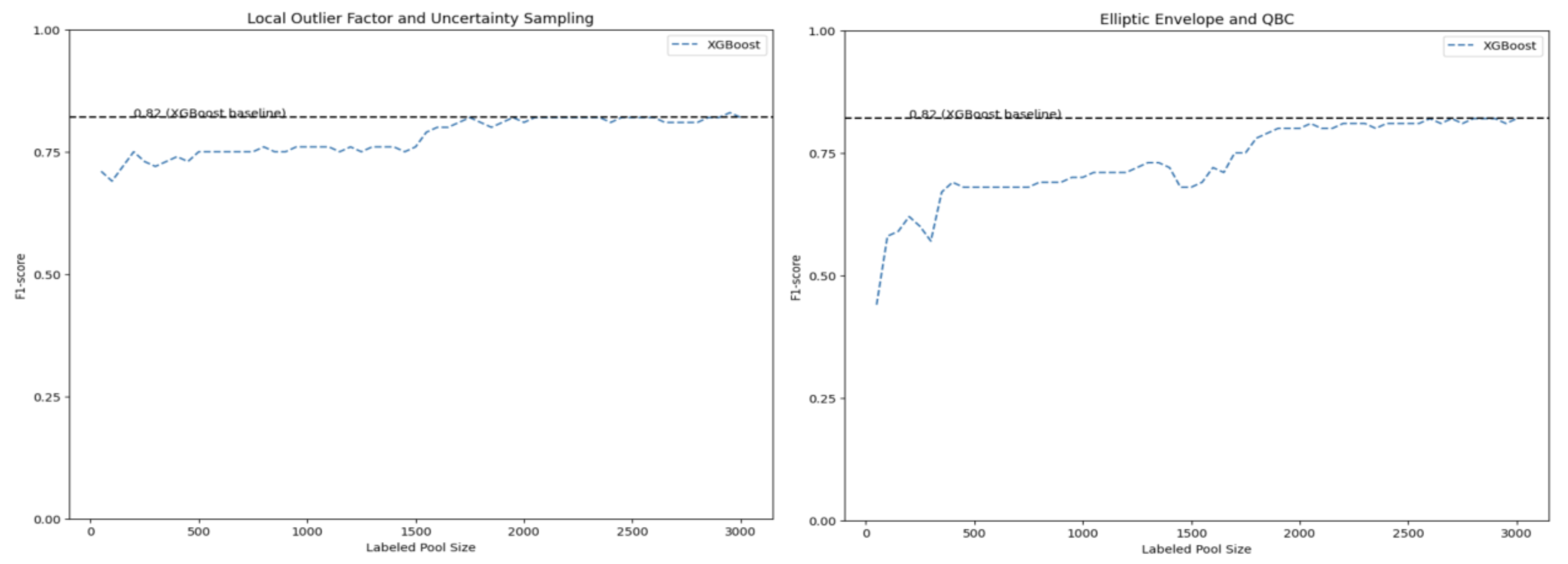
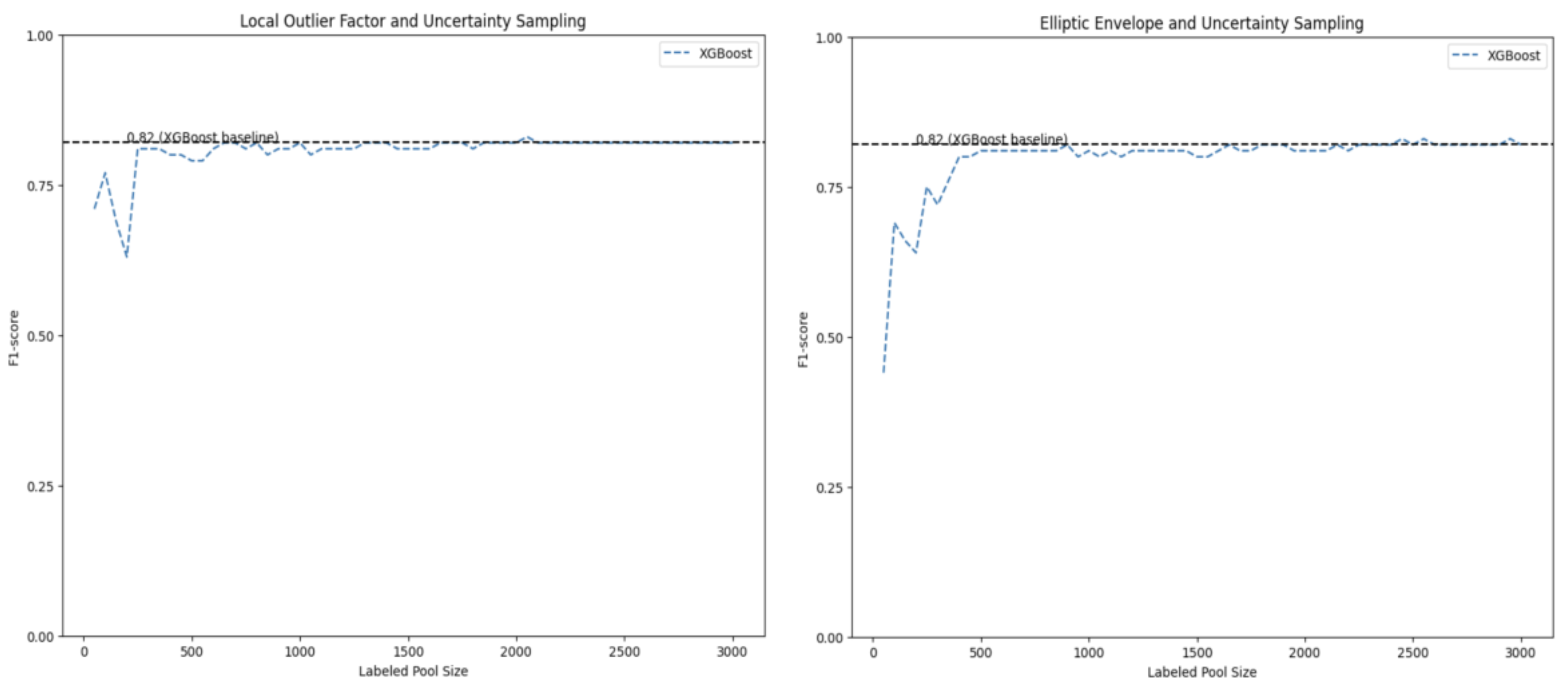
Figure 14 illustrates the evolution of the F1-score across different labeled pool sizes for the best-performing AL setups that utilized XGBoost as a classifier.
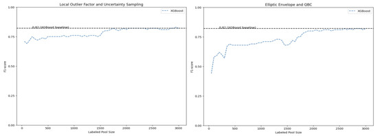
Figure 14.
Learning curves for the best performing Extreme Gradient Boosting setups (cut-off—30th iteration).
Similarly, to what was observed in Figure 13, Figure 14 also visually highlights the accelerated improvement when a supervised AL policy is applied. From what can be visualized, the baseline F1-score from XGBoost can be achieved with as few as 2000 labels.
Table 8 presents the results from the AL setups executed for the LR classifier.
Based on the results presented in Table 8, the application of a supervised AL policy also led to a significant enhancement in the performance of the LR classifier. In specific setups that used LOF and EMC, Elliptic Envelope and QBC, or IF and Uncertainty Sampling, this improvement resulted in an F1-score that even surpassed the baseline. Remarkably, achieving this level of performance required only 3000 labeled data points, which corresponded to a mere 10% of the original labels.
Figure 15 depicts the evolution of the LR classifier performance over the different labeled pool sizes for the best-performing setups.
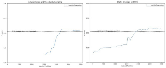
Figure 15.
Learning curves for the best performing Logistic Regression setups (cut-off—30th iteration).
One valuable observation that can be taken from Figure 15 is that the LR classifier exhibited improved performance when trained on a subset of labeled data, but eventually, it tended to converge to its supervised baseline. These findings align with the conclusions drawn in the study conducted by the authors of [14].
The results of the AL setups that were tested considering the usage of unsupervised AL policies exclusively for the initial iteration or until the labeled pool included at least one illicit transaction (i.e., it is necessary to have at least one illicit transaction in the labeled pool to train a supervised classifier) are presented below. This means that the unsupervised AL policies will only be used for the minimum time possible throughout the AL process. The results can be found in Table 9, Table 10 and Table 11, regarding each one of the supervised classifiers.

Table 9.
Results of the active learning setups for Random Forest (cut-off—1st iteration).

Table 10.
Results of the active learning setups for Extreme Gradient Boosting (cut-off—1st iteration).

Table 11.
Results of the active learning setups for Logistic Regression (cut-off—1st iteration).
Table 9 illustrates the results from the AL setups executed for the RF classifier.
Table 9 illustrates the improvement in performance achieved by utilizing only AD algorithms as warm-up learners for a single iteration throughout the AL process.
In comparison to extending the use of AD algorithms for a larger number of iterations, as shown in Table 2 or Table 6, it becomes evident that the supervised baseline of RF, in this case, can be achieved faster, thereby, with minimal labeling. In fact, a near-optimal solution is reached with as few as 1000 labeled transactions, which corresponds to only 3.3% of the original labels in the training set. This earlier transition from an unsupervised warm-up learner to a supervised hot learner leads to improved performance of the RF classifier. This further emphasizes the limited effectiveness of AD algorithms in identifying relevant fraud-related patterns for being queried, while demonstrating the optimal performance of supervised AL policies. This observation aligns with previous findings, as the AD algorithms, given the specific set of features, are unable to accurately identify fraudulent transactions within the unlabeled pool, as these transactions are not anomalous. Therefore, there is no need to extend the use of these techniques throughout the AL process. Once a supervised AL policy is employed, the impact on the performance of the supervised classifier becomes more pronounced.
The findings presented in Table 9 underscore the practical significance of utilizing AL techniques as a cohesive framework. Within this specific context, it becomes apparent that AL allows for attaining performance levels similar to those of a supervised baseline while utilizing a mere 3% of the original labels from the training set. Consequently, the necessity to label an entire dataset for training a supervised classifier is greatly reduced. These results clearly demonstrate that optimal solutions can be achieved by training a supervised classifier exclusively with the most informative transactions obtained through the AL process.
The best-performing setups use LOF and Uncertainty Sampling, and Elliptic Envelope and Uncertainty Sampling. Figure 16 presents the evolution of the RF classifier F1-score over the different labeled pool sizes.
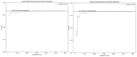
Figure 16.
Learning curves for the best performing Random Forest setups (cut-off—1st iteration).
By comparing Figure 16 to Figure 13, it becomes evident that a swift transition to a supervised AL policy results in a significantly accelerated improvement in the overall performance of the RF classifier. In Figure 13, unsupervised AL policies were employed until the 30th iteration, whereas in Figure 16, a faster transition to a supervised AL policy is observed. As it can be observed, this accelerated transition enables the baseline performance of the RF classifier to be reached faster, requiring only 700 to 800 labels.
Table 10 illustrates the results from the AL setups execution for the XGBoost classifier.
Based on the results presented in Table 10, it becomes evident that the F1-score baseline of the XGBoost classifier is achieved more quickly for the majority of the setups compared to those that continued utilizing an unsupervised AL policy until the 30th iteration. However, it should be noted that when the labeled pool size is limited to only 200 labeled transactions, certain setups that extended the use of unsupervised AL policies (up to the 30th iteration) demonstrated superior performance for that specific pool size (consult Table 7). This could be justified by the fact that supervised policies after being implemented provoke higher variability in the model performance before significantly improving and reaching its respective baseline.
The best-performing setups use LOF and Uncertainty Sampling, and Elliptic Envelope and Uncertainty Sampling. Figure 17 depicts the evolution of the XGBoost classifier F1-score over the different labeled pool sizes.
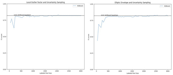
Figure 17.
Learning curves for the best performing Extreme Gradient Boosting setups (cut-off—1st iteration).
Table 11 illustrates the results from the AL setups executed for the LR classifier.
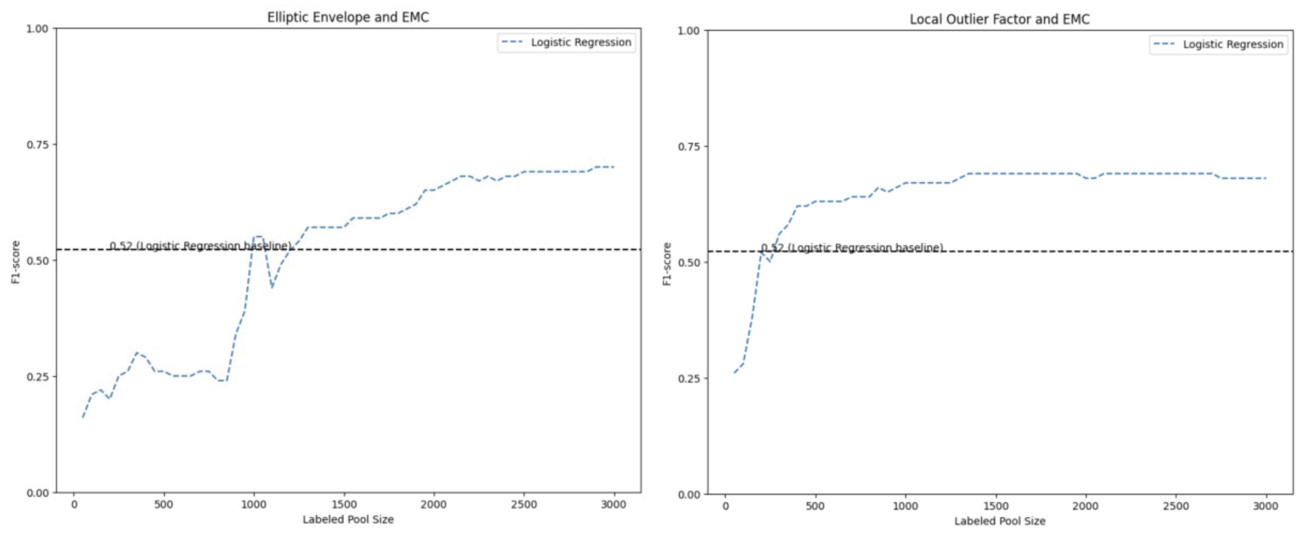
Based on the findings presented in Table 11, several interesting considerations can be made. It is possible to infer that the performance of the LR classifier was also significantly affected when a supervised AL policy was applied immediately after the labeled pool contained one illicit transaction. By minimizing the use of unsupervised AL policy throughout the AL setups, some setups were even able to achieve or even surpass the performance of the supervised baseline using as few as 200 labels, which accounts for only 0.7% of the training set. Notably, for certain setups, LR even outperformed its baseline by 0.15 considering the entire AL process. Consequently, it can be concluded that this particular structure greatly enhanced the LR classifier’s performance. Note that even though LR was able to surpass its own baseline F1-score, it was not able to surpass the best baseline F1-score, which was achieved by RF.
In certain setups, particularly those starting with LOF, it is worth noting that the LR model tends, again, to exhibit improved performance when trained on a sample of the labeled data, but eventually tends to converge to its supervised baseline. This observation further emphasizes the need for implementing early stopping in the AL process.
The best-performing setups used LOF and EMC, as well as Elliptic Envelope and EMC. Figure 18 provides a visual representation of the LR F1-score’s progression across the different labeled pool sizes, showcasing its evolution.
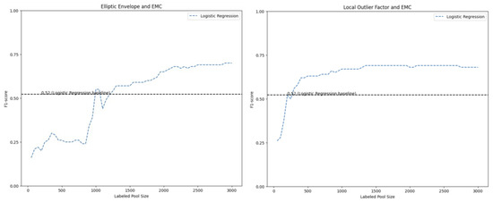
Figure 18.
Learning curves for the best performing Logistic Regression setups (cut-off—1st iteration).
4. Discussion
All of our findings show the subpar performance of AD algorithms in identifying relevant cryptocurrency fraud-related patterns within the unlabeled pool.
A random algorithm would give similar or superior results to AD algorithms for different illicit rate levels. Since AD methods for this specific set of features fail to detect and identify illicit instances correctly, they are highly ineffective at querying illicit transactions to be added to the labeled pool and quickly improving the performance of a supervised classifier.
It has been demonstrated that incorporating AD algorithms in AL configurations fails to yield favorable outcomes regarding the model’s overall performance. Although the AL literature about this topic has already indicated that employing AD algorithms throughout the entire AL setup may not result in optimal performance for a supervised classifier, it would still be anticipated that utilizing AD algorithms would surpass the use of Random Sampling.
These findings highlight the main limitations of AD algorithms that often struggle when faced with illicit activities’ complexity and evolving nature. Therefore, these methods generally have inherent limitations in scenarios where the boundary between normal and illicit behavior is not well-defined. As it was proven, for these specific sets of features in the Elliptic Dataset, there is no clear distinction between normal and illicit behavior, and they have similar patterns.
Evidence was presented that anomalies/outliers in the feature space are not indicative of fraudulent behavior. Therefore, the fact that illicit transactions exhibit various patterns and characteristics that overlap with everyday transactions makes it challenging for AD algorithms to distinguish between the two accurately.
The insights from most of the AD literature review indicate that AD methods can often detect relevant illicit transactions and even previous unknown patterns. The results of this research did not align with those expectations. These findings suggest that studies conducted on synthetic datasets where fraudulent transactions were intentionally designed to be anomalous may lead to unreliable results.
In other words, the bad performance of AD algorithms can be related to the fact that, in the cryptocurrency context, the most deviant transactions are not, in fact, fraudulent ones.
The cryptocurrency market is highly volatile, with prices fluctuating rapidly. This volatility can lead to legitimate transactions that appear anomalous from a static perspective. For instance, large transactions made during periods of high market volatility might seem suspicious, but genuine investment or trading activities could drive them.
The lack of anomalous or deviant patterns in bitcoin transactions associated with illicit activities could also be attributed to fraudsters intentionally imitating normal transaction behavior. This deliberate mimicry poses a significant challenge for anti-fraud algorithms, making it increasingly difficult to accurately identify illicit transactions within the bitcoin cryptocurrency network.
Based on the unsatisfactory performance observed in the unsupervised AL policies, it has been demonstrated that transitioning to supervised AL policies as quickly as possible can significantly enhance the performance of the supervised classifier. This transition allows for the attainment of optimal solutions with as little as 3% of the original training set.
These findings suggest that by adopting a supervised AL policy, as soon as the initial iteration of the AL setup is completed or when at least one illicit transaction is identified and labeled, the performance of the supervised classifier can be markedly improved.
These findings emphasize that AD methods are only effective in addressing the cold start scenario, where no initial labels are available for the AL process. However, from previous considerations, these methods were proven to perform similarly or even worse than the Random Sampling algorithm in resolving this problem. This dispels the notion of their feasibility.
Despite not requiring the analysis of any underlying pattern in the data, the transactions sampled by the Random Sampling algorithm have a more pronounced impact on the performance of a supervised classifier compared to the transactions queried by the AD algorithms.
The prolonged use of unsupervised AD algorithms in the AL process is ineffective. The findings obtained from this study also suggest the practical relevance of using AL techniques as a way to gather the minimum number of labeled instances necessary to achieve a performance close to the supervised baseline, thereby reducing the time and effort required for labeling a large-scale dataset to train a high-performance supervised classifier.
Using AL as a cohesive framework proved very effective at selecting a subset of the data for annotation that maximized the model’s learning potential. Even so, the AD algorithms performed poorly. It is possible that, still, LOF was the only unsupervised algorithm capable of identifying more relevant illicit transactions within the unlabeled pool at different illicit rates. This proves that LOF works better than traditional AD methods at identifying outliers in high-dimensional datasets.
Additionally, among the supervised AL policies that were employed, there is no clear best policy. These supervised AL policies performed very adequately for most of the tested setups.
5. Conclusions
Training a supervised classifier is made easier by utilizing unsupervised AD algorithms and AL strategies to build an iterative process for obtaining labeled transactions. A thorough analysis of the project was carried out, emphasizing a few key ideas. In particular, it looked at how cryptocurrency fraud is changing, how ML techniques are used in the FD field, the fundamentals of AD techniques, and how AL and AD algorithms might work together. A study by [14] was chosen because it offered an appropriate framework for integrating AL and AD algorithms.
The goal of the project was to choose various supervised machine learning models, including LR, XGBoost, and RF, to act as a benchmark for comparing the AL approaches’ performance. The unsupervised AL policies used three algorithms: LOF, IF, and Elliptic Envelope. Furthermore, three supervised AL policies were put into practice, which use supervised models to determine which instances in the unlabeled pool are the most informative. These supervised AL techniques consist of QBC, EMC, and Uncertainty Sampling.
These inferences are made in light of the strategies that have been defined. With a score of 0.83 in the F1-score, RF stood out as the best-performing model out of all the tested models. Furthermore, RF demonstrated remarkable precision, signifying the high accuracy of the optimistic predictions generated by the RF model. It is important to note that although RF performed the best, XGBoost also produced excellent outcomes. Comparing the LR model to the RF and XGBoost models, LR performed worse overall. These results demonstrated how well ensemble approaches, such as RF and XGBoost, handle the subtleties and complexity of cryptocurrency FD.
Two scenarios emerged from the experiments carried out to evaluate the viability of utilizing AD algorithms in AL setups. Throughout the AL process in the first scenario, AD algorithms were used as unsupervised AL strategies. In the second case, supervised and unsupervised AL strategies were combined, and an explicit cut-off point was reached to trigger the switch to a supervised AL policy. The outcomes of these experiments clarified the effects of introducing AD algorithms into the AL procedure and offered information about the ideal cut-off point for moving to a more advanced supervised AL policy.
Regarding the AL experiment scenario wherein only unsupervised AL policies were used during the whole AL process, some conclusions can be drawn. The AD algorithms might have performed better at accurately identifying and detecting a sufficient number of illicit transactions. As a result, these techniques were unable to consistently find pertinent fraud-related patterns in the unlabeled pool for additional labeling, which would have improved the performance of a supervised classifier. These results highlight the shortcomings of AD algorithms, particularly in situations where it is difficult to draw a clear line between acceptable and unacceptable behavior. There were no standout examples in the Elliptic dataset that could be categorically labeled as unlawful.
This leads to two significant conclusions, which were then thoroughly explored. First, it was proposed that the dataset’s mostly bitcoin cryptocurrency transactional nature may be the reason for the lack of glaringly anomalous transactions that would have been indicative of fraudulent activity. From a static perspective, the inherent volatility and dynamics of cryptocurrency markets may cause legitimate transactions to appear anomalous. But rather than being motivated by dishonest intent, these transactions are motivated by real investments and strategic trading activities. This implies that one should carefully consider the apparent abnormality of specific transactions in light of the overall behavior of the cryptocurrency market.
Second, the results suggest that when conducting cryptocurrency transactions, fraudsters may intentionally imitate typical transaction behavior. This finding highlights significant concerns regarding the ways in which criminals conceal their illegal activity by imitating lawful transaction patterns. The outcomes of the second scenario provided further insight into a few more conclusions, given the poor performance of the unsupervised AD algorithms. This scenario led to an important discovery: a supervised classifier performs much better when it switches as early as possible from an unsupervised AL strategy to a more complex supervised AL policy.
Surprisingly, the best solutions were obtained with relatively few labeled transactions (usually between 700 and 800 labels). This underscored the inadequate efficacy of unsupervised AL policies in identifying pertinent transactions from the unlabeled pool. It was even possible to outperform the LR classifier by a significant margin of 0.15 in terms of the F1-score by implementing a supervised AL policy following the completion of one iteration of the AL process. This excellent result highlights the usefulness of using AL techniques as a unified framework to shorten the time and effort needed to label a large-scale dataset in order to train a supervised classifier.
These results also highlighted the fact that AD approaches work best in the cold start situation, in which the AL process has no initial labels. Nevertheless, prior analyses have demonstrated that these approaches either perform on par with or worse than the Random Sampling algorithm when it comes to solving this particular problem. This refutes the idea that they are feasible. The implemented code can be found on GitHub.
At last, the chance to work with precise data from Uphold has presented itself, providing a special opportunity to assess the viability of the suggested methodology with Uphold’s proprietary dataset. The conversations that followed covered a wide range of subjects, such as looking at the dataset itself, feature engineering, and a detailed rundown of the dataset’s advantages and disadvantages.
The largest obstacle in this research was the substantial amount of computational time needed to run the AL setups. Due to the nature of the research, multiple AL setups involving different combinations of supervised and unsupervised AL strategies across a range of cut-off points and supervised classifiers were conducted. As a result, this extensive testing required a significant amount of computational power and was very time-consuming. To solve the aforementioned problem, Uphold supplied a personal computer with improved computational capabilities. It still took a long time to obtain consistent results, though.
In conclusion, this study adds to the growing body of knowledge in the field of financial engineering related to cryptocurrencies by providing valuable information for upcoming research projects aimed at improving the effectiveness of AD and AL methods in this area. Careful analysis and evaluation led to a greater understanding of the underlying mechanisms and variables that might affect their efficacy. For researchers, practitioners, and other stakeholders engaged in creating and putting into practice AD and AL strategies in the cryptocurrency space, this information is essential.
As Future Work Emerges
As future work emerges, we will investigate and evaluate additional unsupervised and supervised labeling strategies and analyze their outcomes, considering the balance between implementation complexity and achieved results. Addressing the following areas can advance the understanding and make more strides in AD and AL: explore other real-life cryptocurrency datasets; conduct an in-depth investigation on the impact of different feature sets on the performance of AD algorithms; investigate graph-embedding techniques that utilize graph information and evaluate their potential to enhance the prediction accuracy of AD algorithms, and finally carry out a study using a quality assurance and control framework for data science projects.
Author Contributions
The manuscript was prepared and revised by all the authors who made significant contributions to the study’s conception and design, up until the point at which it was approved. Data collection, statistical analysis, manuscript preparation, and bibliographical research were handled by A.P.M., D.F.O. and L.L.C.; M.A.B. made a significant contribution to every aspect of the paper, including revision, approval, and the interpretation of the data included in the text. Additionally, each author contributed to the creation of the tool used to collect data. All authors have read and agreed to the published version of the manuscript.
Funding
This work has been supported by FCT—Fundação para a Ciência e Tecnologia within the R&D Units Project Scope: UIDB/00319/2020.
Data Availability Statement
Conflicts of Interest
The authors declare that there is no conflict of interest regarding the publication of this paper.
References
- Nassif, A.B.; Talib, M.A.; Nasir, Q.; Dakalbab, F.M. Machine Learning for Anomaly Detection: A Systematic Review. IEEE Access 2021, 9, 78658–78700. [Google Scholar] [CrossRef]
- Sabry, F.; Labda, W.; Erbad, A.; Malluhi, Q. Cryptocurrencies and Artificial Intelligence: Challenges and Opportunities. IEEE Access 2020, 8, 175840–175858. [Google Scholar] [CrossRef]
- Zhou, H.; Sun, G.; Fu, S.; Wang, L.; Hu, J.; Gao, Y. Internet Financial Fraud Detection Based on a Distributed Big Data Approach with Node2vec. IEEE Access 2021, 9, 43378–43386. [Google Scholar] [CrossRef]
- Shayegan, M.J.; Sabor, H.R.; Uddin, M.; Chen, C.L. A Collective Anomaly Detection Technique to Detect Crypto Wallet Frauds on Bitcoin Network. Symmetry 2022, 14, 328. [Google Scholar] [CrossRef]
- Hilal, W.; Gadsden, S.A.; Yawney, J. Financial Fraud: A Review of Anomaly Detection Techniques and Recent Advances. Expert Syst. Appl. 2022, 193, 116429. [Google Scholar] [CrossRef]
- Barata, R.; Leite, M.; Ricardo Pacheco, F.; Marco P Sampaio, F.O.; João Tiago Ascensão, F.; Pedro Bizarro, F.; Pacheco, R.; P Sampaio, M.O.; Tiago Ascensão, J.; Bizarro, P. Active learning for imbalanced data under cold start. arXiv 2021, arXiv:2107.07724. [Google Scholar]
- Jeyakumar, S.; Andrew Charles, E.Y.; Rathore, P.; Palaniswami, M.; Muthukkumarasamy, V.; Hóu, Z. Feature Engineering for Anomaly Detection and Classification of Blockchain Transactions. TechRxiv 2023. [Google Scholar] [CrossRef]
- vom Brocke, J.; Hevner, A.; Maedche, A. Introduction to Design Science Research. In Design Science Research. Cases; vom Brocke, J., Hevner, A., Maedche, A., Eds.; Springer International Publishing: Cham, Switzerland, 2020; pp. 1–13. [Google Scholar] [CrossRef]
- Vynokurova, O.; Peleshko, D.; Bondarenko, O.; Ilyasov, V.; Serzhantov, V.; Peleshko, M. Hybrid machine learning system for solving fraud detection tasks. In Proceedings of the 2020 IEEE 3rd International Conference on Data Stream Mining and Processing, DSMP 2020, Lviv, Ukraine, 21–25 August 2020; pp. 1–5. [Google Scholar] [CrossRef]
- Trozze, A.; Kamps, J.; Akartuna, E.A.; Hetzel, F.J.; Kleinberg, B.; Davies, T.; Johnson, S.D. Cryptocurrencies and future financial crime. Crime Sci. 2022, 11, 1–35. [Google Scholar] [CrossRef] [PubMed]
- Yang, L.; Dong, X.; Xing, S.; Zheng, J.; Gu, X.; Song, X. An abnormal transaction detection mechanim on bitcoin. In Proceedings of the 2019 International Conference on Networking and Network Applications, NaNA 2019, Daegu, Republic of Korea, 10–13 October 2019; pp. 452–457. [Google Scholar] [CrossRef]
- Jeragh, M.; Alsulaimi, M. Combining Auto Encoders and One Class Support Vectors Machine for Fraudulant Credit Card Transactions Detection. In Proceedings of the 2nd World Conference on Smart Trends in Systems, Security and Sustainability, WorldS4 2018, London, UK, 30–31 October 2018; pp. 57–64. [Google Scholar] [CrossRef]
- Choi, R.Y.; Coyner, A.S.; Kalpathy-Cramer, J.; Chiang, M.F.; Peter Campbell, J. Introduction to Machine Learning, Neural Networks, and Deep Learning. Transl. Vis. Sci. Technol. 2020, 9, 14. [Google Scholar]
- Lorenz, J.; Silva, M.I.; Aparício, D.; Ascensão, J.T.; Bizarro, P. Machine learning methods to detect money laundering in the bitcoin blockchain in the presence of label scarcity. In Proceedings of the ICAIF 2020—1st ACM International Conference on AI in Finance, New York, NY, USA, 15–16 October 2020. [Google Scholar] [CrossRef]
- Xue, Z.; Wang, M.; Zhang, Q.; Zhang, Y.; Liu, P. A regulatable blockchain transaction model with privacy protection. Int. J. Comput. Intell. Syst. 2021, 14, 1642–1652. [Google Scholar] [CrossRef]
Disclaimer/Publisher’s Note: The statements, opinions and data contained in all publications are solely those of the individual author(s) and contributor(s) and not of MDPI and/or the editor(s). MDPI and/or the editor(s) disclaim responsibility for any injury to people or property resulting from any ideas, methods, instructions or products referred to in the content. |
© 2023 by the authors. Licensee MDPI, Basel, Switzerland. This article is an open access article distributed under the terms and conditions of the Creative Commons Attribution (CC BY) license (https://creativecommons.org/licenses/by/4.0/).

