1. Introduction
Spray nozzles play a crucial role in agricultural practices as they are widely used for distributing pesticides, fertilizers, and other treatments to crops. To ensure the effectiveness of agricultural crop spraying systems, it is essential to determine the properties of the droplets sprayed from the nozzles, such as droplet size, velocity, and spray patterns [
1]. These factors directly influence spray retention and drift, which, in turn, have significant impacts on both crop health and the environment [
2]. The effectiveness of crop spraying systems and their treatment performance are intrinsically linked to the dimensions and speed of the sprayed droplets. Hence, precise and accurate measurements of droplet size and velocity are essential prerequisites to optimize nozzle design and enhance the overall efficiency of the spraying process. However, state-of-the-art methodologies for assessing these droplet properties suffer from several problems, including manual and complicated implementation, suboptimal accuracy, and excessive cost.
For instance, one simplistic approach to estimating droplet sizes involves dispersing colored liquid onto a white sheet, which is followed by a subsequent analysis of the resultant patterns to obtain approximate droplet size information. On the other end of the spectrum, a more sophisticated technique, known as the immersion sampling method, employs a silicone oil-coated glass plate to yield more precise measurements of droplet dimensions [
3]. Nonetheless, the traditional methodologies employed for evaluating droplet properties generally involve intricate experimentation, thus incurring high expenses, as well as requiring specialized equipment and skilled personnel to operate [
4,
5].
To address these challenges, this research project proposes an innovative alternative approach grounded in recent advancements in the fields of computer vision and machine learning. Our proposed technique not only enables accurate measurements of droplet size, but also facilitates the real-time detection of droplets in video recordings. By integrating these technological innovations, our method offers promising advantages in terms of accessibility, cost-effectiveness, and reliability, which can significantly contribute to advancing agricultural spray nozzle design and optimizing treatment efficiency.
The methodology employed in this study for droplet detection is rooted in the principles of deep learning, and it is a powerful approach capable of real-time detection of droplet sizes. This droplet detection methodology aims to significantly improve the precision of droplet assessments, even under challenging conditions. A benchmark dataset for droplet detection is introduced in this paper, which facilitates the evaluation of the system’s performance in real-world spraying scenarios. The obtained results substantiate the accuracy and efficiency of the proposed method, underscoring its potential to advance sustainable agricultural practices. Prior to delving into the proposed methodology, the following section provides a review of the existing state-of-the-art research in this domain and identifies their inherent limitations.
2. Literature Review
Particle image velocimetry (PIV) is the current advanced state-of-the-art methodology for measuring the flow of droplets; it is used to visualize and measure fluid velocities in a flow field [
6]. This optical flow measurement technique involves introducing tiny particles into the flow, illuminating them with a laser, capturing consecutive images with a camera, and using image processing software to calculate velocity vectors based on the particle displacements. PIV provides non-intrusive, quantitative data that helps researchers and engineers gain valuable insights into fluid dynamics for various applications. Conventional computer vision techniques coupled with a complicated sensor system were also used for droplet detection on captured images [
7,
8,
9]. However, these existing methods do not offer a solution for measuring the characteristics of individual droplets to estimate their properties. Our hypothesis is that computer vision integrated with recent advances in deep learning may fill this critical gap.
Object detection enabled by deep learning has emerged as a dynamic and intensely investigated domain, garnering notable attention in recent years owing to its remarkable practicality in diverse fields, such as computer vision, robotics, and autonomous vehicles. A plethora of studies have been undertaken in this realm, in which the efficacy of deep learning methodologies for object detection has been delved into. Specifically, the seminal work of Ren et al. (2015) [
10] introduced a region-based convolutional neural network (R-CNN) that incorporates a region proposal network (RPN) to generate potential candidate object regions called Faster R-CNN, which they subsequently classified by a deep neural network. This pioneering approach attained state-of-the-art outcomes across various object detection benchmarks. Other notable approaches for object detection include the YOLO framework proposed in Redmon et al. (2016) [
11], which uses a single neural network to predict bounding boxes and class probabilities directly from full images in real time. In addition to these approaches, several other deep learning-based object detection methods have been proposed, including the Single Shot MultiBox Detector (SSD) [
12], RetinaNet [
13], and Mask R-CNN [
14]. These techniques have demonstrated superior performance in various benchmarks and have been applied in various applications.
Recent research in this field has focused on improving object detection accuracy and efficiency using deep learning. For example, researchers have proposed techniques to optimize deep learning models [
15,
16], explored alternative architectures for object detection [
17], and studied the problem of object detection under challenging conditions, such as in occlusion and changing lighting conditions [
18]. The framework developed by Acharya et al. (2022) [
19] was the first deep learning approach that aimed to address the problem of droplet detection to improve crop spraying systems. This pipeline incorporates four essential components, namely feature extraction, region proposal, pooling, and inference. These components are devised using deep neural networks, convolutional layers, and filters, which are proven to be highly effective in various computer vision applications.
In the context of droplet detection, the work of Wang et al. (2021) [
9] presented a noteworthy development. Their research introduced a highly integrated and intelligent droplet detection sensor system utilizing the MobileNetSSD model. This model, designed for portability, is particularly adept in drone applications for detecting spray droplet depositions. The sensor system developed by Wang et al. incorporates a droplet deposition image loop acquisition device and a supporting host computer interactive platform. Notably, their approach uses an adaptive light model to counter the impact of environmental light on image recognition, thus enhancing field detection capabilities. The MobileNetSSD network, as revealed through their quantitative analysis, successfully balances accuracy and lightweight requirements, making it suitable for embedded devices. Subsequently, the work of Gardner et al. (2022) [
20] stands out, where they employed YOLOv3 and YOLOv5 models for the high-precision monitoring of cell encapsulation in microfluidic droplets. Their approach, capable of processing over 1080 droplets per second, demonstrated the application of deep learning in high-throughput environments and addressed the challenge of class imbalance in training datasets. Their study underscored the versatility of deep learning models in analyzing microfluidic droplets, a context that is significantly different yet conceptually related to agricultural applications.
A notable advancement in the field is the work by Hasti and Shin (2022) [
21]. They proposed a deep learning-based method for denoising and detecting fuel spray droplets from light-scattered images utilizing a modified UNet architecture. Their method represents a significant leap in addressing the challenges of noise and clarity in droplet detection. Their approach, which effectively differentiates droplets from noise, shows potential for the real-time processing of data, a critical aspect in dynamic fluid systems.
Recent advancements in medical imaging segmentation offer valuable insights that can be applied to other domains such as agricultural droplet detection. For instance, Wang et al. (2022) [
22] developed AWSnet, a novel segmentation method for myocardial pathology in CMR data. This method combines reinforcement learning with a coarse-to-fine approach, demonstrating success in accurately delineating complex pathological regions. Such computational techniques may hold potential for enhancing segmentation tasks in agricultural settings. Yu et al. (2022) [
23] addressed the challenges of varying object scales and blurred edges in medical imaging by developing a weakly supervised semantic segmentation method for thyroid ultrasound images. Their approach underscores the complexity and necessity of precision in segmentation tasks. Additionally, Zhou et al. (2023) [
24] introduced DSANet, a dual-branch shape-aware network tailored for echocardiography segmentation in apical views. Their network employs shape-aware modules, including an anisotropic strip attention mechanism and cross-branch skip connections, to enhance feature representation and segmentation accuracy (particularly for cardiac structures such as the left ventricle and left atrium). The integration of a boundary-aware rectification module by Zhou et al. emphasizes the criticality of accurate boundary identification, a principle that could be advantageous in droplet detection. Furthermore, data augmentation techniques have gained significant attention in improving deep learning model performance in medical imaging. Guan et al. (2022) [
25] and Guan et al. (2022) [
26] demonstrated the effectiveness of a novel multichannel, progressive generative adversarial network with texture constraints for pancreas dataset augmentation. Their work highlighted the role of continuous texture and accurate lesion representation in enhancing detection performance, an approach that might be beneficial in the context of agricultural droplet detection.
Our research, while drawing inspiration from these studies, focuses on the agricultural domain, specifically targeting the detection of water droplets in crop spraying scenarios. We employed the YOLOv8 framework to create a robust, accurate, and efficient method for droplet detection. Our approach contrasts with Gardner et al.’s [
20] focus on microfluidic droplets and Wang et al.’s emphasis on lightweight model deployment. We address the challenges in existing methodologies, such as occlusions and variations in droplet size and shape, with advanced deep learning techniques. Furthermore, we have developed an autonomous annotation method for large-scale droplet data and optimized our model for embedded systems, thereby extending the feasibility for real-time implementations in mobile crop spraying systems. In comparison to Acharya et al. (2022) [
19], the key improvements of this work include the following:
The droplet detector in [
19] was designed to strike a balance between processing speed and achieving higher accuracy. In the current work, we show that it is possible to achieve even higher accuracy while reducing the processing speed.
The data annotation in [
19] was carried out manually. Manual labeling of droplet data is not practical in real-world settings, especially when dealing with large volumes of data. In this work, we developed a method for autonomous annotation of droplet data.
The pipeline discussed in [
19] can only operate with a high-performance computing cluster. In this work, we propose a model pruning technique to substantially reduce the number of parameters, thereby shortening the processing time and making it deployable in embedded systems. This opens up the feasibility for real-time implementations in mobile crop spraying systems.
Therefore, the main goal of this work is to create a more robust, accurate, compact, and faster inference pipeline for droplet detection.
Statement of Contributions
We leverage deep learning and computer vision to detect the motion of droplets from sprayed nozzles moving across camera frames in real time. Our algorithm is grounded in the recent progress in state-of-the-art detection methods, such as YOLOv8 and model pruning, to improve droplet detection precision and enable real-time operation. We address several challenges in the previous work of [
19], including occlusion and variations in droplet size and shape. To overcome the occlusion problem, we implemented a robust algorithm that utilizes deep learning models capable of capturing and interpreting complex visual patterns, even in the presence of occlusions. By leveraging these methods, we are able to accurately detect droplets, even when they are partially obscured or hidden behind other droplets. Furthermore, we addressed the challenge of variations in droplet size and shape by developing a flexible and adaptable framework. Our approach incorporated adaptive learning mechanisms that enable the model to dynamically adjust its detection parameters based on the characteristics of the droplets observed in the input data. This allowed our system to effectively handle variations in droplet size and shape, ensuring accurate and reliable detection results across different scenarios and conditions.
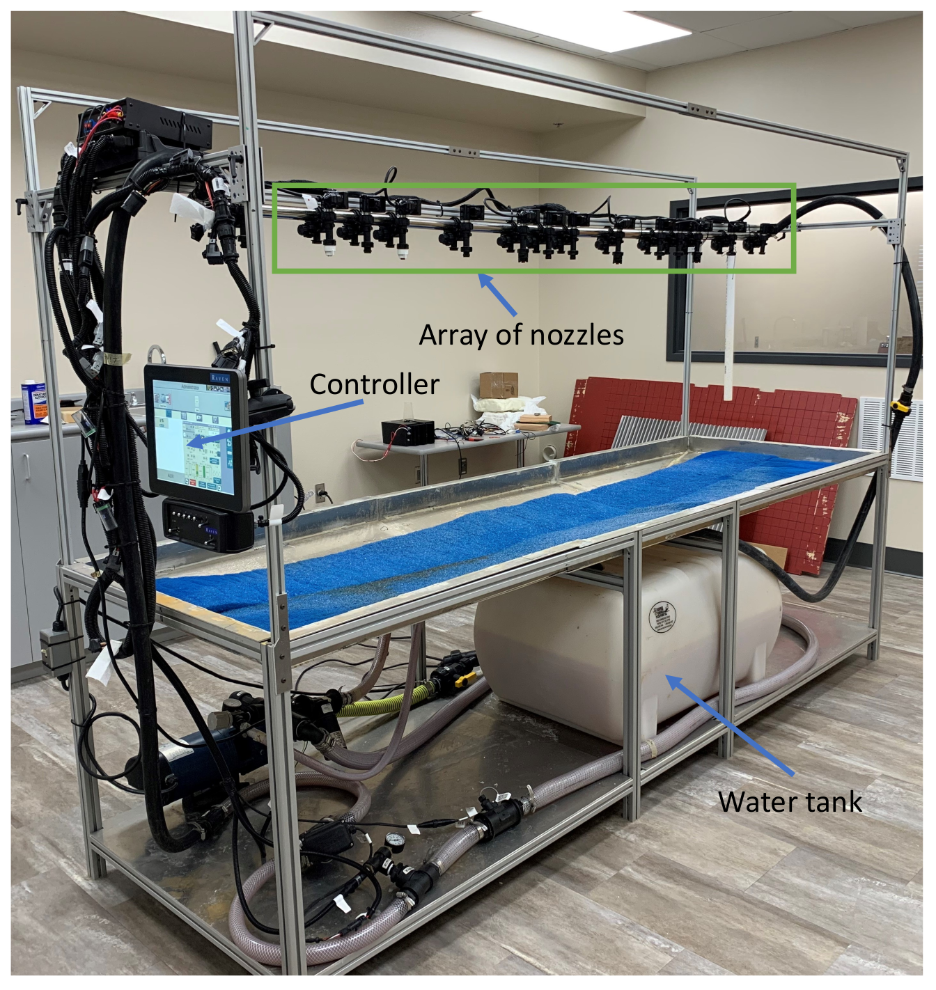
The experimental data utilized in this study were collected through a dedicated setup featuring crop spraying nozzles, as illustrated in
Figure 1. The data collection process was conducted via a user interface controller, which regulated the flow rate of the water pumped from the water storage tank to the nozzles. The setup comprises an array of nozzles capable of producing different spray patterns. To record droplet motion, an Olympus i-SPEED 3 camera (Tokyo, Japan) with a frame rate of 2000 fps and a lighting system were positioned beneath the nozzles. However, annotating the data posed a tremendous challenge because there were thousands of droplets to be labeled in order to construct a sufficiently large ground truth dataset for training. To address this challenge, this work proposes a method for automatic annotation, which results in an accurately labeled and substantial dataset.
The key contributions of this work are summarized as follows:
Design and implementation of a real-time droplet detection approach that achieves a higher level of accuracy.
An AI-enabled automatic labeling and augmentation tool for establishing big droplet datasets.
The innovative modification of state-of-the-art models for droplet detection to optimize their performance with respect to speed and precision, thereby facilitating the practical implementation of our method.
Overcoming the limitations associated with previous droplet detection frameworks, such as in [
19], as discussed earlier.
Implementing a framework on an onboard computer platform, Jetson Orin, as well as enabling advanced mobile robotics and edge AI capabilities for droplet analysis.
3. Real-Time Deep Learning-Based Droplet Detection
3.1. Overview of the Methodology
The methodology in this paper builds upon the recent architecture provided by YOLOv8 [
27] to deliver a higher precision and faster processing rate compared to the state-of-the-art methods in droplet detection. The selection of YOLOv8 is underpinned by several key theoretical considerations:
Enhanced Speed and Real-time Processing: YOLOv8, as a single-stage detector, inherently offers faster processing speeds, which is crucial for real-time applications in agricultural spraying where immediate feedback is essential.
Robust Accuracy in Diverse Conditions: Our dataset includes complex backgrounds and varying lighting conditions. YOLOv8’s architecture maintains high detection accuracy in these diverse conditions, which is an important consideration mirrored in our methodology.
Effective Detection of Small Objects: The precise detection of small droplets is a critical aspect of our study. YOLOv8 improves feature extraction and bounding box prediction mechanisms, thereby providing enhanced capabilities in detecting small droplets.
YOLOv8’s design is particularly beneficial for detecting small, fast-moving objects like droplets as it effectively addresses challenges such as varying sizes and overlapping objects. The use of YOLOv8 allows for the integration of advanced features like multi-scale prediction and a more refined anchor box mechanism, which are vital for accurately identifying droplets in diverse conditions. In particular, the process is shown in
Figure 2 and encompasses the following key steps:
Preprocessing: The input image is resized and normalized to values between 0 and 1.
Feature Extraction: A total of 53 convolutional layers were created to extract a series of feature maps, which were then unified via a feature pyramid network (FPN) for detecting droplets across various sizes.
Detection Head: The unified feature map was passed to the detection head, which is composed of convolutional and fully connected layers. It predicts bounding boxes, objectness scores, and class probabilities for droplets, which are respectively classified into large, medium, and small sizes. Anchor boxes were also utilized here, which helped in identifying droplets with diverse dimensions.
Anchor Boxes: As seen in
Figure 3, the anchor boxes were predefined to cover different droplet sizes and shapes, thus aiding in predicting precise locations and sizes.
Non-Maximum Suppression (NMS): Finally, NMS was applied to reduce overlapping bounding boxes, and only those with the highest objectness score within each overlapping region were retained.
The rest of the section will be dedicated to elaborating on the technical details of these steps.
The rest of the methodology section will delve deeper into the key aspects of the droplet detection framework.
3.2. Feature Extraction
The backbone network used in this work is composed of a series of convolutional layers that extract features from input images. These convolutional layers use filters or kernels to perform a series of convolutions on the input image. The output of each convolutional layer is a set of feature maps that represent different levels of abstraction in the input image.
Early Layer Feature Maps: The initial layers predominantly focus on low-level features. These include the following:
- -
Edges: Refers to the sharp changes in intensity or color in the image and marks the boundaries of objects within the field of view.
- -
Textures: Patterns or repetitive arrangements found on the surface of objects in the image, often manifesting as fine details.
Later Layer Feature Maps: Advanced layers capture more complex, high-level features. These encompass the following:
- -
Shapes: Refers to the geometric or outline properties of objects, as well as captures the overall form and structure of the droplets.
- -
Boundaries: A more holistic view of the contours of objects, and it also helps to distinguish the droplets from the background by recognizing their complete periphery.
To improve the efficiency of the feature extraction process, we used the CSPNet architecture [
28] to split the input feature maps into two parallel paths, which were processed separately and then merged back together. This approach allowed us to reduce the number of computations required while still maintaining the accuracy of the predictions. The algorithm was designed in such a way that the feature extraction process was followed by a series of upsampling and concatenation operations to increase the resolution and combine the feature maps from different layers. The resulting feature maps were then used to predict bounding boxes and class probabilities for droplets in the image.
For example, when a droplet image of a size of
pixels is input, it goes through a series of convolutional layers. These layers gradually down sample the image to sizes of
,
, and finally
pixels. Furthermore, it then extracts features at different abstraction levels like edges, textures, shapes, and boundaries. The feature maps are subsequently processed through additional convolutional layers, restoring them to the original input dimensions of
pixels. These final feature maps are used to predict the bounding boxes and class probabilities for the droplets in an image. As demonstrated in
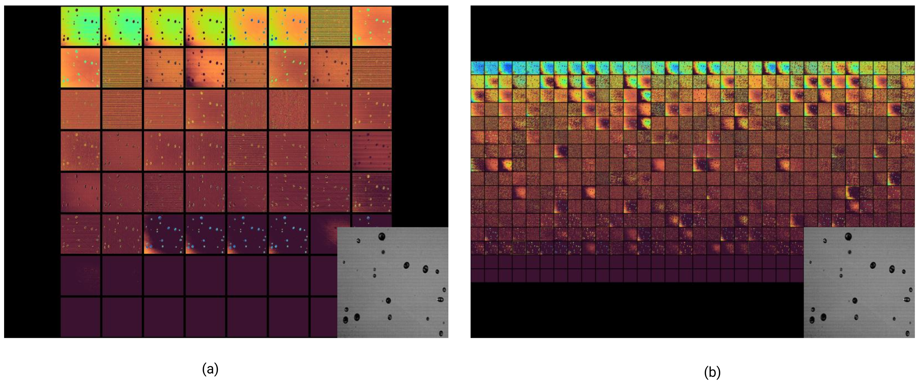
Figure 4, this process of feature extraction produces clearly identifiable patterns.
Figure 4 displays the feature extraction from a droplet image, in which the distinct patterns on the feature maps are highlighted. The left panel shows the early layer’s feature maps, and it focuses on low-level, specific details like edges and corners with low spatial resolution. The right panel represents the last layer’s feature maps, whereby more abstract, high-level features like shapes and boundaries with higher spatial resolution are captured. These varying feature maps contribute to tasks like droplet detection and classification, with clear distinctions between the early and final layers in terms of resolution, receptive field, and abstraction level being made.
3.3. Detection Head
The detection head plays a critical role in the droplet detection framework in this paper. It is a set of layers added on top of the backbone network that takes the high-level features extracted by the backbone and performs droplet detection by predicting the bounding boxes’ offsets and associated class probabilities. The droplets are classified into three size-based categories: large, medium, and small.This classification is derived from their physical dimensions, as follows:
Small Droplets: Droplets with sizes up to the 33rd percentile of the size range in our dataset. In our study, this threshold is defined as 299.0 units.
Medium Droplets: Droplets whose sizes fall between the 33rd and 67th percentiles, representing the mid-range sizes.
Large Droplets: Droplets exceeding the 67th percentile, which, in our dataset, corresponds to a size of 525.0 units and above.
These thresholds were calculated based on the percentile distribution of droplet sizes within our dataset, thus helping to ensure an empirical and data-driven approach to categorization.
The class probabilities represent the probability that the droplet in the anchor box belongs to a particular class, while the offsets represent the distance between the anchor box and the ground truth bounding box. These parameters are predicted using a series of convolutional layers that transform the input feature maps into a set of feature vectors. The class probabilities are predicted using a sigmoid activation function and are normalized such that they sum to 1 across all classes:
where
is the probability that the droplet in the anchor box belongs to class
c,
is the sigmoid activation function,
is the weight vector for class
c, and
is the feature vector for the anchor box.
Each anchor box is associated with a set of offsets, which are represented by a vector of 4 elements encoding the distance between the anchor box and the ground truth bounding box. The offsets are predicted using a linear activation function applied to the coordinates of the anchor box to obtain the coordinates of the predicted bounding box via the following equation:
where
and
are the predicted coordinates and dimensions of the bounding box;
and
are the coordinates of the center of the anchor box;
and
are the dimensions of the anchor box;
and
are the weight vectors for the offsets; and
is the feature vector for the anchor box.
After the bounding boxes are predicted, the post-processing module applies non-maximum suppression (NMS) to remove the redundant bounding boxes that overlap with each other. The NMS algorithm applies an intersection over union (IoU) threshold to the class probabilities (Equation (
1)) and removes all bounding boxes that have a lower probability (IoU) than the threshold. It then selects the bounding box with the highest probability for each droplet class and removes all other bounding boxes that have a high overlap with the selected bounding box. IOU measures the overlap between the predicted bounding box and the ground truth bounding box of a droplet. It is calculated as the ratio of the area of intersection between the two bounding boxes,
i and
j, to the area of their union as follows:
where
and
are two bounding boxes,
is the intersection of the two boxes,
is the union of the two boxes, and
is the intersection over union between the two boxes.
3.4. Optimization-Driven Model Training
The process of training a model is crucial in deep learning to tune the hyperparameters that enable the model to produce predictions as close to the ground truth as possible. During this phase, the model learns to identify patterns and make predictions based on the ground truth data. In the context of our droplet detection system, the model needs to be trained to recognize droplets of different sizes and shapes and to track their movement across frames. The training process involves feeding the model with labeled data, which contain images of droplets with their corresponding bounding boxes and class labels. The model then automatically adjusts its parameters to minimize the difference between the predicted droplet detections and the ground truth droplet labels. This process is iterative and continues until the model’s performance on the training data reaches a satisfactory level or until a specified number of iterations (epochs) have been completed.
In this work, the training process for the deep learning model was formulated as an optimization problem, as described in
Figure 5, where the objective is to find an optimal set of model parameters that minimize a loss function. The loss function quantifies the difference between the predicted and actual labels for the training data. In the case of our droplet detection system, we designed the loss function as a combination of the following:
Localization Loss (
): This loss is calculated using the intersection over union (IoU) between the predicted bounding box and the ground truth bounding box. The IoU is a measure of the overlap between two bounding boxes and is calculated using Equation (
6). The localization loss is then calculated as
Classification Loss (
): This loss is calculated using the cross-entropy loss between the predicted droplet class score (
) and the ground truth droplet class labels (
). The equation for weighted cross-entropy loss is
Here,
- -
The outer summation iterates over the detected droplets.
- -
The inner summation iterates over the classes.
- -
is 0 or 1, and it corresponds to whether the ground truth class of a detected droplet i is class j or not. Specifically, if the true class for the detected droplet i is class j, otherwise .
- -
represents the predicted score that the detected droplet i belongs to class j. This score is used as an input to the sigmoid function to convert it into a predicted probability for the corresponding class.
- -
and are hyperparameters that exist within the range [0,1].
- -
represents the sigmoid function , where .
Confidence Loss (
): This loss is calculated using the binary cross-entropy loss between the predicted objectness score (
) and the ground truth objectness score (
). The equation for the binary cross-entropy loss is
The total loss (
L) is then a weighted sum of the following three losses:
where
,
, and
are the weights for the localization loss, classification loss, and confidence loss, respectively.
The model parameters are then tuned automatically via the stochastic gradient descent scheme to minimize the following loss function:
where
is the learning rate,
is the gradient of the loss with respect to the parameters, and
is a randomly selected index from
at iteration
t.
The training process also involves a validation dataset, which is a separate set of data that is not used in the initial training phase. We split our data into three sets: training, validation, and testing. The training set was used to adjust the model parameters, while the validation set was used to tune the hyperparameters and monitor the model’s performance during the training process. The performance of the model on the validation set was monitored during the training process to prevent overfitting (i.e., the model performs well on the training data but poorly on unseen data). The training process was stopped when the performance on the validation set stopped improving. After the training and validation phases, the final model was evaluated on the testing set. This set was completely unseen during the training and validation phases, and it also provided a measure of how well the model will perform on real-world data.
3.5. Model Pruning
The initial deep neural networks designed in this work have a large number of connections and weights, which lead to tremendous computational and memory demands during training and deployment. To alleviate the demands, we implemented a model pruning technique to reduce the complexity of the neural networks by removing redundant connections and weights, thus making the codes easier to load, store, and deploy. Since the resulting model is substantially more compact and efficient, it can be trained and deployed even with resource-constrained devices such as embedded systems and onboard computers. Additionally, the smaller model also leads to energy and memory efficiency gains, which are crucial for battery-powered devices such as smartphones or drones [
29]. In this section, we will describe the pruning procedures detailed in Algorithm 1.
| Algorithm 1 Pseudo-code for model pruning with a threshold. |
Input: Trained neural network model, pruning threshold - 1:
Initialization: - 2:
Let W be the set of weights in the model - 3:
Let S be an empty dictionary to store importance scores - 4:
Compute Importance Score: - 5:
for each weight do - 6:
ComputeImportanceScore(w) ▹ Use a criterion like L1 and L2 - 7:
end for - 8:
Prune Weights: - 9:
for each weight do - 10:
if then - 11:
▹ Prune the weight - 12:
end if - 13:
end for - 14:
Fine-tune Model: - 15:
Train the model with the remaining weights using a reduced learning rate - 16:
Repeat: - 17:
If the desired level of compression is not achieved, return to step 4.
Output: The pruned and fine-tuned neural network model |
Compute the importance score: This step involves computing an importance score for each layer, neuron, or weight in the model based on a specific pruning criterion. The pruning criterion can be based on various factors, such as weight magnitude, sensitivity analysis, or information entropy. The importance score represents the contribution of each layer/neuron/weight to the overall performance of the model, and it is used to determine which connections/weights to prune. In this work, we employed the weight magnitude parameter to compute the importance scores of weights in the model pruning process. The process of how weight magnitude can be used to compute importance scores is as follows:
Compute the Magnitude of the Weights: The algorithm computes the magnitude of each weight in the neural network by taking the absolute value of the weight and disregarding its sign.
Normalize the Magnitudes: The algorithm normalizes the magnitudes of the weights by dividing each weight’s magnitude by the maximum magnitude observed across all weights in the model. e.g., . This step ensures that the magnitudes are scaled between 0 and 1, thus allowing for a fair comparison among the weights.
Importance Score Calculation: The importance score of a weight can be directly derived from its normalized magnitude by assigning the normalized magnitude as the importance score for weight w.
Prune the least important connections/weights using the pruning threshold: After computing the importance scores, the least important connections/weights are pruned based on a pruning threshold. The pruning threshold represents the threshold value used to determine which connections/weights to prune based on their importance scores. Connections/weights with importance scores below the pruning threshold are considered unimportant and are pruned by setting the weight value to zero. The pruning process aims to remove redundant connections/weights and reduce the size of the model while maintaining its accuracy.
Fine tune the pruned model to recover the performance loss caused by pruning: After pruning, the model is fine tuned to improve the accuracy of the pruned model and mitigate the performance loss caused by pruning. The fine tuning process involves training the model on the same dataset as the original model using a smaller learning rate before pruning.
Algorithm 1 describes the entire model pruning process, including the computation of importance scores, pruning, and fine tuning. Meanwhile, Algorithm 2 focuses specifically on the computation of the importance scores of each weight in the model, which is an essential step in the model pruning process. The importance score represents the contribution of each weight to the overall performance of the model, and it is used to determine which weights to prune during the model pruning process.
| Algorithm 2 Pseudo-code explaining the calculation of importance scores. |
Input: Trained neural network model - 1:
Initialize an empty dictionary to store the importance scores of each weight - 2:
for each layer in the model do - 3:
-norm of weights: - 4:
-norm of weights: - 5:
Store the norm value in the dictionary for each weight in the layer - 6:
end for - 7:
Normalize the importance scores by dividing by the total number of weights in the model
Output: The importance scores of each weight in the model |
The first step of the algorithm initializes an empty dictionary to store the importance scores of each weight in the model. Next, the algorithm computes the -norm or -norm of the weights in each layer of the neural network. The -norm and -norm are mathematical formulas that measure the magnitude of a vector (in this case, the weights in a layer) in different ways. The -norm represents the sum of the absolute values of the weights, while the -norm represents the square root of the sum of the squares of the weights. The importance score of each weight is then computed using the -norm or -norm value computed in the previous step. The importance scores represent the relative importance of each weight compared to other weights in the same layer, and they are then stored in the dictionary initialized in the first step. Finally, the importance scores are normalized by dividing each score by the total number of weights in the model. Normalizing the scores ensures that the importance scores are between 0 and 1, which facilitates the pruning process. The output of the algorithm is the importance score of each weight in the model.
4. Annotation and Augmentation of Experimental Data
In order to create the optimal deep learning-based droplet detection model, we established a dataset that satisfies the following specific requirements:
Diversity of Droplet Characteristics: Ensuring variations in the droplet sizes, shapes, and orientations.
Image Quality and Variation: Images are collected under various conditions.
Multiple Droplet Instances: Including images with more than one droplet.
Sufficient Training Data: An adequate number of images for training, validation, and testing.
4.1. Autonomous Labeling
To meet these requirements, we conducted experiments and collected images/videos of droplets sprayed from an array of nozzles (see
Figure 1 for the experiment setup), as well as created a database with all the images for training, validation, and testing. However, constructing a large-scale dataset of droplets is a time-consuming and resource-intensive process, mainly because it involves the manual labeling of thousands of droplets. The manual annotation also poses challenges in terms of efficiency, accuracy, and scalability. Thus, there is a critical need for an automatic labeling tool to be integrated with the deep learning model. This tool could then alleviate the burden of manual annotation by automating the process and improving the precision and efficiency of labeling.
In order to develop this automatic labeling tool, first, we manually labeled a small set of droplet data to train the droplet detector designed in the first part of this paper. Then, we used this pre-trained model to localize and classify the droplets, thereby assigning appropriate bounding boxes and class labels automatically. Since the droplet detector was trained with a small dataset, there were errors in the droplet detection. Hence, the last step in the process was to manually correct these errors. Although manual annotation was still involved, it was reduced to a manageable task, and the automatic labeling tool bore the main burden of annotation. The tool significantly reduced the time and effort required for dataset annotation, thus allowing us to create large-scale datasets more efficiently. This efficiency is crucial when dealing with thousands or even millions of droplet instances. Since the droplet detector worked so well at that point, there was no manual annotation involved in the data annotation for the model training at all.
4.2. Data Augmentation
We also implemented data augmentation techniques, such as Cutout, Noise, and Mosaic, to increase the dataset’s size and diversity. These techniques were tested for their impact on the mean average precision (mAP), with the Mosaic augmentation technique being the most effective.
Figure 6 illustrates these augmentations.
In the pursuit of enhancing the dataset’s size and diversity, these data augmentation techniques were employed and analyzed for their impact on the mean average precision (mAP). As can be seen in
Table 1, the baseline results, obtained without applying any augmentation, served as a starting point for comparison, with mAP50 values of 0.792 for validation and 0.884 for the test. Applying a 5% noise yielded significant improvements, whereby mAP50 values of 0.904 and 0.903 for the validation and test, respectively, were achieved. The Cutout technique, involving the removal of 10% of the random sections from the images, also demonstrated improvement, with mAP50 values of 0.834 and 0.922 for the validation and test, respectively. Most strikingly, the Mosaic augmentation technique was particularly effective as it achieved superior metrics when compared to the other augmentation techniques with mAP50 values of 0.977 and 0.967 for the validation and test, respectively. However, a combined approach using Noise, Cutout, and Mosaic did not outperform the individual techniques, with mAP50 values of 0.893 for validation and 0.858 for the test. The previous model without augmentation was also evaluated, which achieved a test precision of 0.908. The results clearly indicated that the Mosaic augmentation technique is the most effective method among those tested as it consistently achieved the highest mAP50 and mAP50-95 values. Therefore, the Mosaic augmentation technique was selected as the optimal choice for improving the classification and detection outcomes in this project.
4.3. Data Organization
Figure 7 and
Figure 8 provide insights into the dataset characteristics. This new collection was twelve times larger than that which was previously used, and it encompassed various complexities like varying lighting conditions, multiple droplets, and high droplet density. In
Figure 7a, the aspect ratio distribution of the images within our dataset is portrayed, which provides insights into the diversity of the image dimensions before any standardization process.
Figure 7b presents an annotation heatmap that visualizes the density and distribution of droplets across the standardized image frames. The heatmap employed a color gradient to signify the frequency and location of the droplets. Cooler colors (blues and greens) indicate the areas with a lower likelihood of droplet presence, thus representing fewer annotations and a sparser occurrence of droplets. Warmer colors (yellows and reds) delineate the regions with a higher likelihood of droplet detection, and they correspond to a higher density of annotations. This heatmap effectively illustrates the spatial distribution of droplets within the image frames, and it provides a visual summary of the most and least common locations for droplet occurrence in our dataset.
In the construction of our dataset, we have considered a range of complexities to ensure a robust evaluation of the droplet detection algorithm. As illustrated in
Figure 8, our dataset encompasses the following various challenges:
(a) Different lighting conditions that can significantly affect the appearance of droplets and potentially the performance of detection algorithms. These conditions range from uniform illumination to more complex scenarios with shadows and highlights.
(b) Scenes with multiple droplets, which present the challenge of detecting each droplet accurately while also distinguishing between overlapping droplets.
(c) High droplet density, where the number of droplets in a single frame can be substantial, thus requiring the algorithm to maintain high precision and recall despite the increased difficulty.
These complexities are representative of real-world conditions that any effective droplet detection system must handle. Regarding the construction of a benchmark dataset, the images used in this study are part of a dataset funded and managed by the USDA National Institute of Food and Agriculture. Due to data sharing agreements and privacy constraints, we are unable to make the dataset publicly available. However, we provide representative images from the dataset in
Figure 8, which demonstrate the variety and complexity of the imaging conditions under which our droplet detection system was tested and validated.
6. Experimental Results
6.1. Droplet Datasets
We have discussed various evaluation metrics for droplet detection extensively thus far. As we delve into the results obtained by our trained model in this section, we will be using some specific variants of the mean average precision (mAP) metric, which may fit better for performance evaluation depending on the scenarios. Specifically, we will use mAP50, which refers to the mAP calculated at an intersection over union (IoU) threshold of 0.50; this means that a prediction is considered correct if its bounding box has at least a 50% overlap with the ground truth bounding box. We also used mAP50-95, which is the average of mAP values calculated at IoU thresholds ranging from 0.50 to 0.95 with a step size of 0.05. This gave us a more comprehensive view of the model’s performance across a range of precision levels.
Table 2 shows the experimental results that indicate the comparisons made among the four different datasets and two different models. The models in the comparison include the framework designed in this work and the model developed in [
19]. The datasets include the following:
Previous dataset: The dataset used to produce the results reported in [
19] with the respective model. This dataset includes 468 images in the training set, 41 images in the validation set, and 44 images in the testing set.
Augmented dataset: This is obtained by performing a Mosaic augmentation on the previous dataset to increase the size of the training set to 1404 images.
New dataset: This is obtained by implementing data augmentation and automatic labeling to increase the size to 6124 images in the training set, 494 images in the validation set, and 275 images in the testing set.
The performance was evaluated using precision, recall, mAP50, and mAP50-95 on both the validation and test sets.
6.2. Results on Performance Metrics
We can see from
Table 2 that our model (i.e., the model designed in this work) trained with the Previous dataset, without any augmentation, had the lowest performance as it achieved a validation mAP50 of 0.792 and a test mAP50-95 of 0.526. When trained with the Augmented dataset with Mosaic augmentation, our model achieved a better performance with a validation mAP50 of 0.976 and a test mAP50-95 of 0.624. Additionally, when our model was trained with the New dataset, also with Mosaic augmentation and automatic labeling, it had the best performance, whereby it achieved a validation mAP50 of
and a test mAP50-95 of
. The precision reached
, i.e., the model could successfully detect
of the droplets in the testing set that it has never seen before. Moreover, all these performances were superior when compared to the model developed in [
19], which was trained with the Previous dataset.
The comparison of the results showed that the data augmentation and the design of the model are crucial for achieving good performance in the droplet detection task. The model designed in this paper when coupled with the Mosaic data augmentation outperformed the other models, and the use of the Augmented dataset improved the performance significantly. The results demonstrated that choosing the right combination of dataset, augmentation, and model can lead to a state-of-the-art performance in droplet detection.
Table 3 presents a detailed evaluation of the droplet detection model’s performance across different droplet classes (i.e., small, medium, or large), as well as an aggregate of all the classes. Furthermore, the table also offers insights into various aspects of the model’s effectiveness. The metrics are provided for both validation and test datasets. The following results were particularly noteworthy:
For small droplets, the model’s performance showed a consistent behavior between the validation (precision: 0.846 and recall: 0.92) and test sets (precision: 0.891 and recall: 0.898). The mAP50 values were 0.929 for the validation set and 0.934 for the test set, while the mAP50-95 values were 0.64 and 0.621, respectively. The consistency and relatively high precision and recall values suggested effectiveness in identifying small droplets, but the gap between the mAP50 and mAP50-95 values indicated a sensitivity to IoU thresholds.
In the case of medium droplets, the precision dropped slightly from 0.845 in the validation set to 0.813 in the test set, while the recall values were 0.854 and 0.858, respectively. The mAP50 values were 0.918 for the validation set and 0.912 for the test set, with mAP50-95 values at 0.761 and 0.724, respectively. This indicates that the model maintained a balance between the precision and recall, but there was also a slight drop in the precision in the test set.
For large droplets, the analysis showed consistency between the validation (precision: 0.927 and recall: 0.881) and the test sets (precision: 0.921 and recall: 0.844). The mAP50 values were 0.95 for the validation set and 0.939 for the test set, with mAP50-95 values of 0.792 and 0.751, respectively. The higher precision for large droplets and the closer values between mAP50 and mAP50-95 suggested a robustness to different IoU thresholds.
The aggregate metrics for all the classes showed a precision of 0.873 and a recall of 0.885 for the validation set, as well as a precision of 0.875 and a recall of 0.867 for the test set. The mAP50 values were 0.932 for the validation set and 0.929 for the test set, with mAP50-95 values of 0.731 and 0.699, respectively. These numbers provided a well-rounded view of the model’s performance across all droplet sizes, thus indicating overall stability and generalization ability.
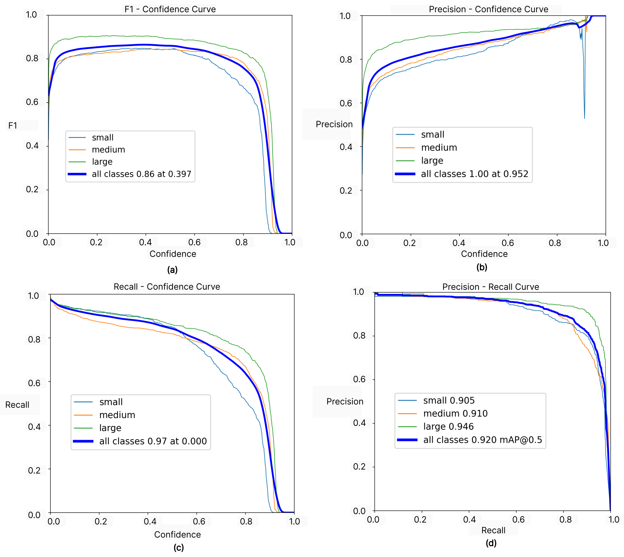
Figure 9 provides a visualization of the training performance of our model when trained with the New dataset, which also achieved the best performance, as shown in
Table 1.
Figure 9a illustrates the F1-confidence curve of our detection model across the different droplet sizes, namely small, medium, and large. The F1 score is a crucial metric in the field of machine learning and computer vision, particularly in tasks such as object detection, where the balance between precision and recall is vital. It provides a single metric that encapsulates the performance of the model in terms of both precision and recall. We can see that the high F1 scores ranging from 0.6 to 0.9 with a confidence threshold from 0 to 0.8 for all classes—including small, medium, and large droplets—are indicative of the model’s strong performance. The model’s performance was consistent across different droplet sizes, as evidenced by the close proximity of the F1 scores for the small, medium, and large droplets. This consistency was maintained over a wide range of confidence thresholds, thus indicating the model’s robustness in handling droplets of various sizes. The F1 scores exhibited a fast increase with a confidence threshold of 0 to 0.1, after which they stabilized up to a confidence threshold of 0.8. This suggests that the model’s performance remains steady over a wide range of confidence levels, thus reinforcing its reliability. However, a drastic decrease in the F1 scores was observed at a confidence threshold above 0.8. This is a common phenomenon in object detection models, as a confidence threshold close to 1 implies absolute certainty in the predictions, which is rarely achievable in practice due to inherent uncertainties and potential errors in the data or model.
The precision, which indicates the proportion of true droplets (i.e., correct detections) among all detected droplets, was used as a measure of the model’s performance. Regarding the precision–confidence curve, as shown in
Figure 9b, for small droplets, the precision started at 0.5 and then rapidly climbed to 0.7 at a confidence level of 0.08. This suggests that the model’s accuracy in predicting small droplets quickly improves as the confidence level increases. When the confidence level is between 0.1 and 0.85, the precision is rising gradually for all classes of droplets. However, a sudden drop in precision from above 0.9 down to 0.5 was observed at a confidence level of about 0.9, which was followed by a rebound to 1 at a confidence level close to 1, for the small droplets. This volatility suggests that the model’s performance on small droplets may be less stable at high confidence levels, which could potentially be due to the inherent challenges associated with smaller droplets. In contrast, the precision for medium and large droplets exhibited a steady increase for the majority of the precision–confidence curve. The absence of any sudden drops in precision indicates that the model’s performance on medium and large droplets is stable across all confidence levels and its performance improves consistently as the confidence level increases.
The recall–confidence curve of our model was analyzed to understand the model’s performance across various droplet classes, including small, medium, and large. Recall, which is defined as the ratio of true positive predictions to the sum of true positives and false negatives, serves as an essential metric through which to gauge the model’s ability to correctly identify the droplets it was trained to detect. Regarding the recall–confidence curve, as shown in
Figure 9c, for small droplets, the recall commences at 1 at a confidence level of 0, which gradually diminished to 0.5 at a confidence level of 0.8. This gradual decline illustrates the model’s decreasing efficacy in identifying small droplets as the confidence level rises. A precipitous decline to a 0 recall at a confidence level of 1 underscores a potential vulnerability in the model’s performance with small droplets at elevated confidence levels. Simultaneously, the trend for the medium droplets mirrored that of the small droplets, which initiated at 1 at a 0 confidence and further attenuated to 0.7 at a 0.8 confidence. The less pronounced decline compared to decline in the small droplets indicates a more robust performance with medium-sized droplets, though the trend still suggests a diminishing ability to identify these droplets as the confidence increases. In addition, the recall trajectory for large droplets begins at 1 at a 0 confidence, which then tapers to 0.8 at a 0.8 confidence. This pattern, with the highest recall at a 0.8 confidence among the three sizes, signifies the model’s relative strength in detecting large droplets.
The precision–recall curve is a valuable tool for understanding the trade-off between precision (the ratio of true positive predictions to the sum of true positives and false positives) and recall (the ratio of true positive predictions to the sum of true positives and false negatives). The precision–recall curve, as shown in
Figure 9d, demonstrated that both the small and medium droplets exhibited a similar trend in terms of precision and recall. As the recall increased from 0.0 to 0.8, the precision gradually decreased from 1.0 to 0.9. This gradual decline illustrated that, as the model identified more droplets (increasing recall), it became slightly less accurate in its predictions (decreasing precision). The decrease in precision for the small and medium droplets implied a balanced trade-off between these two metrics for these droplet sizes. Meanwhile, the large droplets followed a similar pattern but with a milder decline in precision. Starting at 1 precision with 0 recall, the precision decreases to 0.95 at a recall of 0.8. This higher precision at the same recall level compared to small and medium droplets suggests that the model is more accurate in detecting large droplets.
6.3. Results of the Confusion Matrix and Training Loss
Figure 10 presents the confusion matrix for the three classes of droplets of our droplet detection model. The model correctly identifies 92% of the small droplets but misclassified 8% as medium. For the medium droplets, the model showed good performance with an 85% true positive rate, but it also had some confusion between the small and large categories. Large droplets were identified with an 87% true positive rate, with some confusion with the medium category and an 18% false positive rate with the background. The model’s performance with large droplets stood out as particularly strong, while there were areas of confusion between the small and medium categories.
In addition to the mAP metrics, we also evaluated the training loss of our droplet detector, as indicated by the lost functions defined in Equations (
7)–(
10). The training loss provided insights into how well the model is learning from the training data and is an essential aspect of understanding the model’s convergence and overall performance.
Figure 10 illustrates the results of training the droplet detection model over 200 epochs. It includes three types of loss: localization loss, classification loss, and confidence loss. The localization loss started at 1.68 and gradually decreased to 0.52 by the end of the training. This indicated that the model’s ability to accurately locate droplets within an image improved over time. The consistent decrease in the localization loss suggested that the model was learning the spatial characteristics of the target droplets effectively. The classification loss began at 1.93 and ended at 0.29. This metric measures the model’s ability to correctly classify the droplets within the image. The substantial reduction in classification loss over the epochs indicated that the model was becoming increasingly proficient at identifying the correct classes for the droplets. Simultaneously, starting at 1.06, the confidence loss dropped down to 0.8 after 200 epochs. Confidence loss typically measures the model’s certainty in its predictions. The decrease in this loss shows that the model’s confidence in its predictions improved but at a slower rate when compared to the other two losses. This is because the features that describe large, medium, and small droplets are very similar to each other, especially if the size differences are subtle.
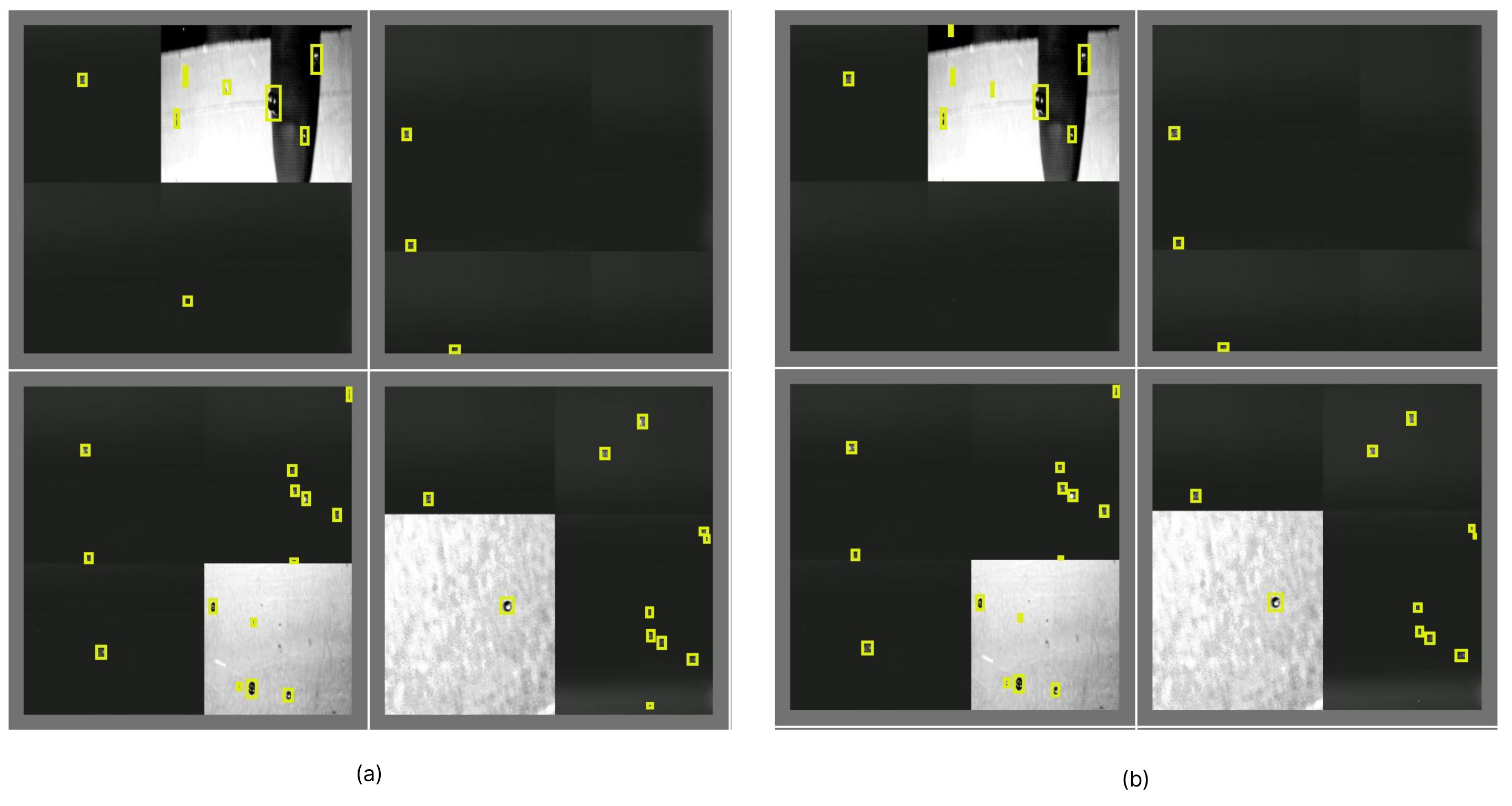
Figure 11a consists of the labeled ground truth images, which contain multiple bounding boxes that denote the droplets.
Figure 11b shows the detection results on the right, and it highlights the droplets detected by the model with high confidence scores (>0.9). The confidence score represents the level of certainty or confidence assigned by the model to each detected droplet. It indicates the model’s confidence in the accuracy of the detection, with higher scores indicating a stronger belief that the droplet is present. Notably, the detection results, as shown in
Figure 11b, encompassed all of the droplets present in the ground truth data, which is shown in
Figure 11a. Interestingly, the model can even detect additional droplets that do not have corresponding bounding boxes that the ground truth data missed. It appears that the droplet detection model achieved an exceptional performance, in which it potentially indicated convergence and exhibited a high level of effectiveness.
It is also evident from
Table 2 that our model, when trained with the Previous dataset without any augmentation, demonstrated the least robustness to occlusion. In contrast, the model trained with the Augmented dataset, when using Mosaic augmentation, exhibited an improved performance, which was evidenced in it maintaining high mAP50 values even with partial droplet occlusions. The model trained with the New dataset, which included Mosaic augmentation and automatic labeling, showcased the highest resilience to occlusion with only a marginal decrease in the mAP50-95 when faced with up to 50% occlusion. The consistent precision and recall across varying levels of occlusion underscore the model’s ability to detect and correctly classify partially visible droplets, which is a critical aspect for real-world applications where occlusions are commonplace. In addition, in
Figure 11b, we present a series of image patches that showcase the droplet detection model’s capacity to recognize droplets under varying conditions, including instances of partial occlusion. This robust detection even amidst occlusions can be attributed to the model’s learned feature representations, which are capable of capturing the essential characteristics of droplets even when they are not fully visible. The ability to discern partially obscured droplets is crucial for applications in dynamic environments, where complete visibility of every droplet cannot always be guaranteed. The results depicted in
Figure 11b affirm the model’s proficiency in maintaining high detection accuracy—a testament to its robustness against occlusion.
The excellent performance of the model can be attributed to its advanced architecture, effective training process, and robust feature representation. The model’s deep neural network structure allows for the efficient and precise detection of droplets, whereby it leverages multi-scale features to capture intricate details. Through extensive training, the model has learned to effectively discriminate between droplets and background regions, thereby resulting in accurate and comprehensive detection. The convergence of the model’s training process, coupled with its ability to generalize in unseen instances and handle various droplet sizes, enables it to surpass expectations and achieve a desirable performance in droplet detection tasks.
6.4. Results of Model Pruning and Implementation in an Embedded System
Table 4 and
Table 5 demonstrate the inference time of the droplet detection and tracking framework before and after pruning, which were measured in milliseconds per frame on different devices with distinct GPU and CPU configurations. The pruning process described in Algorithm 1 resulted in a more compact model with approximately a 30% reduction in the model size. This was achieved by removing the redundant or less significant parameters, connections, and layers. The compactness makes the model compatible with mobile onboard computers.
The observed improvements in the inference time before and after pruning are as follows:
For the Jetson AGX Orin device, the CPU inference time improved by approximately 4.9% after pruning, while the GPU inference time remained almost the same with a reduction of approximately 0.4%.
In the case of the AI supercomputer, both the CPU and GPU inference times improved after pruning. The CPU time decreased by approximately 1.3%, while the GPU time decreased by approximately 8.4%.
On the work station, there were slight improvements in both the CPU and GPU inference times after pruning. The CPU time reduced by approximately 0.8%, and the GPU time reduced by approximately 7.8%.
The improvements in inference time after pruning can be attributed to several factors. Pruning removes redundant parameters and reduces memory access and computational complexity. This leads to optimized computation, increased parallelism, and streamlined execution, thus resulting in faster inference times. These findings suggest that the performance of the droplet detection framework can be optimized through pruning, thereby resulting in more efficient processing of frames, especially with GPUs. However, it is worth noting that the specific GPU and CPU configurations of each device also play a role in determining the overall inference time. The percentage reductions in inference time after pruning indicate an improved efficiency and faster processing of droplet detection. These improvements contribute to better performance and near real-time capabilities. This makes the droplet detection framework more practical and efficient for deployment in various mobile applications.
Upon further analysis, we recognized that the nuances of GPU inference on the Jetson AGX Orin platform required additional explanation, especially in the context of model pruning. Unlike more powerful AI supercomputers and workstations, the Jetson AGX Orin is designed with a focus on power efficiency for embedded systems. As such, the pruning process, while reducing the model’s complexity, does not significantly impact the already optimized GPU inference due to the embedded system’s limited parallel processing resources when compared to full-scale GPUs.
The Jetson AGX Orin’s embedded GPU is tailored for high efficiency in a constrained power envelope, and this architectural focus on efficiency means that there is less redundant computation to eliminate through model pruning. Therefore, the performance gains on this platform from pruning are more noticeable on the CPU than the GPU. This contrasts with more powerful, dedicated GPU platforms, where the larger number of parallel processing cores can benefit from the reduced computational load post-pruning. Furthermore, it should be noted that the observed marginal reduction in GPU inference time on the Jetson AGX Orin could be within the range of measurement variability, thus suggesting that the performance on such embedded systems can be primarily constrained by hardware capabilities rather than model complexity.
7. Conclusions
This study represents a pioneering step in the field of droplet detection, and it exhibits an innovative methodology grounded in deep learning and an architecture laid by YOLOv8. By leveraging cutting-edge techniques—such as CSPDarknet53 for feature extraction, non-maximum suppression for clutter-free detection, and model pruning to make it compact—our approach significantly enhances the precision and processing rate in droplet detection. The use of anchor boxes and unification through a feature pyramid network further contributes to the model’s ability to detect droplets across various sizes with solitary, optimally situated bounding boxes.
The experimental results, which showcase a 97% precision and 96.8% recall in droplet detection, affirm the advantages of our methodology. Moreover, its capability of real-time operation on embedded systems like Jetson Orin makes it a viable and revolutionary tool for practical applications in agriculture. Our approach thus provides a foundation for sustainable farming practices by facilitating efficient resource utilization and waste reduction.
This research not only sets a new benchmark in droplet detection, but it also opens up promising avenues for further exploration and refinement. Future work can delve into extending the applicability of this model to other domains and enabling more efficient pixel processing by integrating policy networks and reinforcement learning into the droplet detection framework. We are also working toward making this technology deployable in mobile crop spaying systems in the field.


