Article

SHapley Additive exPlanations (SHAP) for Efficient Feature Selection in Rolling Bearing Fault Diagnosis

by
Mailson Ribeiro Santos
1,*,
Affonso Guedes
2 and
Ignacio Sanchez-Gendriz
3
1
Postgraduate Program in Electrical and Computer Engineering, Technology Center, Federal University of Rio Grande do Norte, Natal 59078-970, Rio Grande do Norte, Brazil
2
Department of Computer Engineering and Automation, Federal University of Rio Grande Do Norte, Natal 59078-970, Rio Grande do Norte, Brazil
3
Laboratory for Technological Innovation in Health (LAIS), Hospital Universitário Onofre Lopes, Federal University of Rio Grande Do Norte (UFRN), Natal 59078-970, Rio Grande do Norte, Brazil
*
Author to whom correspondence should be addressed.
Mach. Learn. Knowl. Extr. 2024, 6(1), 316-341; https://doi.org/10.3390/make6010016
Submission received: 5 October 2023 / Revised: 30 November 2023 / Accepted: 4 December 2023 / Published: 5 February 2024
(This article belongs to the Special Issue Advances in Explainable Artificial Intelligence (XAI): 2nd Edition)

Abstract

:
This study introduces an efficient methodology for addressing fault detection, classification, and severity estimation in rolling element bearings. The methodology is structured into three sequential phases, each dedicated to generating distinct machine-learning-based models for the tasks of fault detection, classification, and severity estimation. To enhance the effectiveness of fault diagnosis, information acquired in one phase is leveraged in the subsequent phase. Additionally, in the pursuit of attaining models that are both compact and efficient, an explainable artificial intelligence (XAI) technique is incorporated to meticulously select optimal features for the machine learning (ML) models. The chosen ML technique for the tasks of fault detection, classification, and severity estimation is the support vector machine (SVM). To validate the approach, the widely recognized Case Western Reserve University benchmark is utilized. The results obtained emphasize the efficiency and efficacy of the proposal. Remarkably, even with a highly limited number of features, evaluation metrics consistently indicate an accuracy of over 90% in the majority of cases when employing this approach.

1. Introduction

Contemporary industries grapple with a myriad of challenges, particularly those arising from complex operating environments and extensive equipment fleets [1]. Rolling element bearings (REBs) constitute a fundamental component within rotating machinery, making them susceptible to frequent failures that can lead to machine breakdown [2,3]. Consequently, monitoring the health of these machines has become paramount to ensure operational reliability and efficiency. This imperative extends to tasks such as fault detection and diagnosis (FDD), where timely identification of issues is crucial.
Various methods, including vibration, acoustics, temperature, and lubricant analysis, are employed to analyze bearing faults [4,5,6,7]. The prevalent approach to monitoring the health of rotating machines relies on analyzing vibration signals [8]. Machine learning (ML) techniques have proven instrumental in building FDD models, where the input data comprise features extracted from these monitored signals [9]. These features encompass a range of time, frequency, and time-frequency domain measurements, including statistical parameters like mean, standard deviation, maximum, and minimum values in the time domain, as well as components and coefficients of fast Fourier transform (FFT) and discrete wavelet transform (DWT) in the frequency and time-frequency domains, respectively, [10].
While machine learning models such as artificial neural networks (ANNs), support vector machines (SVMs), and k-nearest neighbor classifiers have leveraged these features to identify bearing faults [11], this approach has drawbacks. Feature selection, often decided through trial and error, greatly influences the classification algorithm’s success [12]. Thus, efficient and accurate FDD models necessitate meticulous feature selection [13].
In the pursuit of concise and accurate solutions, a three-phase methodology is presented to address the challenges of fault detection, classification, and severity level estimation in rolling bearings.This sequence of phases operates in a cascading manner, where insights gleaned from the previous phase play a pivotal role in shaping the subsequent one. In the classification phase, only data from the preceding phase, specifically those related to detected faults, are employed. Subsequently, the estimation of severity for each unique fault class.
In recent decades, artificial intelligence (AI) models have emerged as a pivotal technology, driving groundbreaking innovations across various application domains [14]. However, the pursuit of these innovations has sometimes come at the expense of poor model interpretability. Traditional machine learning (ML) algorithms are known for their relatively high explainability, albeit with potentially lower predictive performance. In contrast, more advanced algorithms like deep learning models exhibit greater predictive power but remain challenging to interpret, especially within complex systems. To address this challenge, researchers have introduced explainable artificial intelligence (XAI) [15]. XAI encompasses a range of techniques designed to render the decision-making processes of AI systems understandable and transparent for human comprehension [16].
The objective of XAI is to elucidate the raison d’être of AI systems, discern their capabilities and constraints, and forecast their future evolution [16]. Among the diverse array of XAI methods are notable approaches like LIME, LORE, anchors, occlusion, permutation feature importance, Shapley feature importance, SHAP (Shapley additive explanations), guided backpropagation, DeepLift, and deconvolution [17].
In the context of this paper, from an assortment of methodologies within the realm of XAI, the technique chosen for exploration was SHAP. This technique derives its inspiration from the tenets of cooperative game theory, with particular emphasis on the concept of Shapley’s value—an evaluative mechanism that apportions value to each participant within a coalition, mirroring their contributions to the overall coalition’s end result. When transplanted into the domain of ML, SHAP undertakes the responsibility of quantifying the individual significance of features (inputs) in relation to specific model predictions. This methodology gauges the extent to which the presence or absence of each feature shapes the intended outcome, contrasting it against its absence [18]. This approach is classified as a category of explanatory importance, underscoring the pivotal role played by these features [17].
In this context, the fault detection and diagnosis (FDD) models exclusively employed time domain features in conjunction with the support vector machine (SVM) technique. Nevertheless, the framework proposed possesses a level of generality that accommodates the utilization of alternative feature sets and diverse ML techniques. The proposal is validated using the well-known Case Western Reserve University benchmark for rolling bearing faults [19].
The subsequent sections of this paper are structured as follows: In Section 2, fundamental concepts are elucidated, encompassing FDD, feature selection for ML models, explainable artificial intelligence (XAI), and the application of SHAP (Shapley additive explanations). In Section 3, an in-depth exposition of the three-phased FDD methodology is presented. Section 4 delves into a comprehensive case study utilizing the renowned Case Western Reserve University benchmark for detecting faults in rolling element bearings. This involves an explication of the experimental setup, followed by a meticulous analysis of the resultant outcomes. Lastly, the conclusive remarks and discourse on the findings are presented in Section 5.

2. Theoretical Background

This section aims to provide the essential concepts that underpin a comprehensive understanding of this study. It encompasses critical themes such as FDD and feature selection within machine learning (ML) models.

2.1. Fault Detection and Diagnosis

The escalating complexity of industrial processes over recent decades, driven by market demands, heightened production rates, and stringent environmental and safety regulations, has posed challenges to human operators in overseeing these complex systems [20]. In this context, operator-induced errors account for a substantial proportion—around 70% to 90%—of accidents within industrial environments [21,22]. This reality underscores the pressing need for automated monitoring of operational quality and health, a pivotal endeavor within the Industry 4.0 framework [23].
The health monitoring of industrial system operations fundamentally revolves around the identification and diagnosis of anomalous scenarios that may arise during their functioning [24]. Many of these anomalies stem from equipment faults or disruptions within the system, posing potential threats to the overall performance, integrity, and safety of the entire system. Consequently, fault detection and diagnosis (FDD) activities assume a pivotal role in ensuring the operational efficiency of industrial systems and equipment [25]. Specifically, fault detection involves the task of identifying the occurrence of a fault, whereas fault diagnosis encompasses determining the nature and severity of the fault (encompassing fault classification and severity estimation). Additionally, fault diagnosis endeavors to pinpoint the origin of the fault through techniques such as root cause analysis (RCA) [26]. In the context of this study, FDD encompasses activities related to fault detection, classification, and severity estimation.
FDD methods can be effectively grouped into three main categories: quantitative model-based methods, qualitative model-based methods, and data-based methods. Model-based techniques emanate from a profound understanding of the fundamental physics governing the monitored process. In the case of quantitative methods, this understanding is translated into mathematical relationships that establish connections between the inputs and outputs of the analyzed system. In contrast, data-based methods capitalize on process variable data to fuel their analytical processes. Notably, recent research has prominently favored data-based approaches, primarily due to their autonomy from intricate process dynamic models and their adeptness at harnessing the abundant data resources available today [21].
These data-based FDD models commonly employ ML techniques. During the nascent stages of integrating ML techniques into FDD, traditional feed-forward neural networks were employed as seen in works such as [27,28]. Subsequently, a myriad of ML approaches emerged to engineer FDD models tailored specifically for industrial systems, as highlighted in [29]. A comprehensive investigation conducted by [30] delves deeply into this realm, presenting an extensive exploration that focuses on FDD achieved through ML techniques and their application to rotating machinery.

2.2. Feature Selection of ML Models

In the context of machine learning (ML) models, features serve as the inputs that drive the predictive power of the model. The process of feature selection entails the identification and curation of an optimal set of features that contribute to the construction of effective models, as highlighted by [31]. Given the inherent sensitivity of these models to the quality of information fed into their inputs, the task of feature selection assumes a paramount role in ensuring the efficiency and accuracy of ML models [32].
Diagnosing faults in rotating machines conventionally involves monitoring vibration signals within the machine shaft, as noted by [11]. These ML-based fault detection and diagnosis (FDD) models rely on the distinct characteristics of these signals, which can be extracted from the time domain, frequency domain, or time-frequency domain. In the time domain, typical attributes include mean, root mean square, standard deviation, peak to peak, minimum and maximum values, crest factor, kurtosis, and skewness values [10,33,34,35,36,37,38,39]. Features in the frequency domain often encompass coefficients obtained from the fast Fourier transform (FFT) of the vibration signals, as indicated by references such as [40,41]. In the realm of time-frequency techniques, notable methods include the short-time Fourier transform (STFT) [42,43,44], discrete wavelet transform (DWT) [45,46,47,48,49,50], envelope analysis [2,51,52,53], and empirical mode decomposition (EMD) [54,55,56,57].
The process of feature reduction comprises two primary procedures: feature extraction (transformation) and feature selection. Feature extraction methods, including principal component analysis (PCA), linear discriminant analysis (LDA), and multidimensional scaling, function by transforming the initial features into a new set derived from their combinations, as highlighted by [58]. The objective is to unveil more insightful information within this newly generated set. However, techniques centered around dimensionality reduction introduce new inputs to models, which can escalate processing demands and potentially compromise their explainability by discarding original features during the reduction process.
Conversely, feature selection involves the extraction of a concise subset of features from the original set, all without undergoing transformation. This preserves their inherent interpretability. Subsequently, this selected subset is assessed in light of the analytical objective. The process of selection can be carried out through a range of approaches, contingent on factors such as the precise objective, resource availability, and the desired level of optimization, as outlined by [59]. Feature selection plays a pivotal role in achieving machine-learning-based FDD models that are effective and precise, often demanding an intricate understanding of the system. The literature offers a wide spectrum of techniques for feature selection, including approaches like information gain, chi-square, feature weighting, k-means, localized feature selection based on scatter separability (LFSBSS), Fisher score, and inconsistency criterion, as outlined by [59]. This work will now delve into the realm of feature selection, focusing on an approach that augments explainability while circumventing the introduction of additional processing overhead to the FDD model.

2.3. Explainable Artificial Intelligence (XAI)

The pervasive adoption of ML techniques in various systems facilitates data-driven decision-making, the harnessing of big data solutions, the formulation of effective commercial strategies, the augmentation of process automation, and the mitigation of errors, risks, and operational expenses, among other benefits. However, a significant contemporary challenge revolves around comprehending the decision-making mechanisms of these ML models. This becomes particularly crucial in domains where the outcomes of these decisions bear sensitivity, as in applications involving human subjects [60].
To gain deeper insights into the decision-making processes of ML models, the field of explainable artificial intelligence (XAI) has emerged [17]. The primary objective of XAI is to introduce and employ techniques that yield more interpretable models or enhance their explainability, all while preserving their commendable performance levels [61].
The landscape of XAI has witnessed remarkable expansion, transforming from a niche research topic within AI into a dynamic and multidisciplinary field. This evolution is a direct response to the growing success of ML, especially deep learning (DL), in real-world applications. XAI emerges as a pivotal force in addressing the escalating need for transparency in AI systems. As AI, and particularly DL models, become increasingly prevalent in diverse domains, the challenge of understanding these complex and opaque systems has become more pronounced. XAI methods play a critical role in enhancing the interpretability of AI models by tailoring explanations specifically to the cognitive needs of human stakeholders. These methods, including the provision of social, contrastive, and selective explanations, contribute to making the decision-making process of AI models more comprehensible to a wider audience. The focus on transparency and interpretability empowers stakeholders to grasp the contributing factors and features that underpin AI model predictions or decisions, fostering a clearer understanding of the technology’s impact. As XAI continues to advance, collaborative efforts and interdisciplinary research aim to align research agendas and explore promising directions, harnessing the collective intelligence of diverse stakeholders to further enhance the understandability of AI models [62].
XAI techniques can be categorized based on three key criteria: (I) the degree of interpretability complexity, (II) the extent of interpretability coverage, and (III) the level of reliance on the chosen ML model [63]. Typically, simpler models are more readily interpretable, while highly complex models present challenges in terms of interpretation and explanation. Concerning the scope of interpretability, these methods are commonly classified into two subcategories: global interpretability and local interpretability. Global interpretability aims to unveil the entirety of a model’s logic and delineate the reasoning processes that lead to its various possible outcomes. On the other hand, local interpretability focuses on elucidating specific decisions or significant predictions within the model [63].
Agnosticism constitutes a crucial attribute in characterizing XAI techniques. Agnostic approaches possess the capability to be employed across diverse types of ML algorithms or models [63]. Consequently, such XAI techniques are highly advantageous as they can seamlessly integrate with a wide range of ML methodologies.
The Shapley value, originally conceptualized to assess the significance of individual participants in cooperative team settings, has found application in the realm of machine learning through the SHAP (Shapley additive explanations) library. Rooted in game theory, the Shapley value mechanism seeks to equitably distribute the cumulative benefit of collaborative efforts among participants based on their relative contributions to the final outcome [64].
One of the key strengths of SHAP is its versatility, making it applicable to a wide range of ML models, from simple linear models to complex deep neural networks. This flexibility is essential in the diverse landscape of modern ML, where models of varying complexity are employed for different tasks [18]. SHAP’s agnostic nature allows it to be seamlessly integrated into different frameworks, providing a consistent methodology for interpreting model outputs.
The core idea behind SHAP is to assign a Shapley value to each feature, quantifying its marginal contribution to the model’s prediction for a given instance. The Shapley value, originally devised to fairly distribute the benefits among participants in a cooperative game, is adapted in SHAP to allocate the model’s output to individual features in a way that reflects their relative importance. This approach is particularly valuable for complex models where the contribution of each feature is not immediately apparent [65].
In practical terms, SHAP achieves this by considering all possible combinations of features and their contributions, evaluating the model’s output for each combination. The Shapley values are then computed by averaging over all possible orders in which features are added to the combination. This process provides a fair and consistent attribution of the model’s output to each feature, unveiling their individual impacts on the final prediction.
Among the variety of plots available in the SHAP library, this study will exclusively analyze the summary plot. This plot adopts a beeswarm plot format, comprising multiple dots. Each dot encapsulates three essential features. For instance, an illustrative example of a summary plot can be observed in Figure 1. The attributes of each dot are as follows:
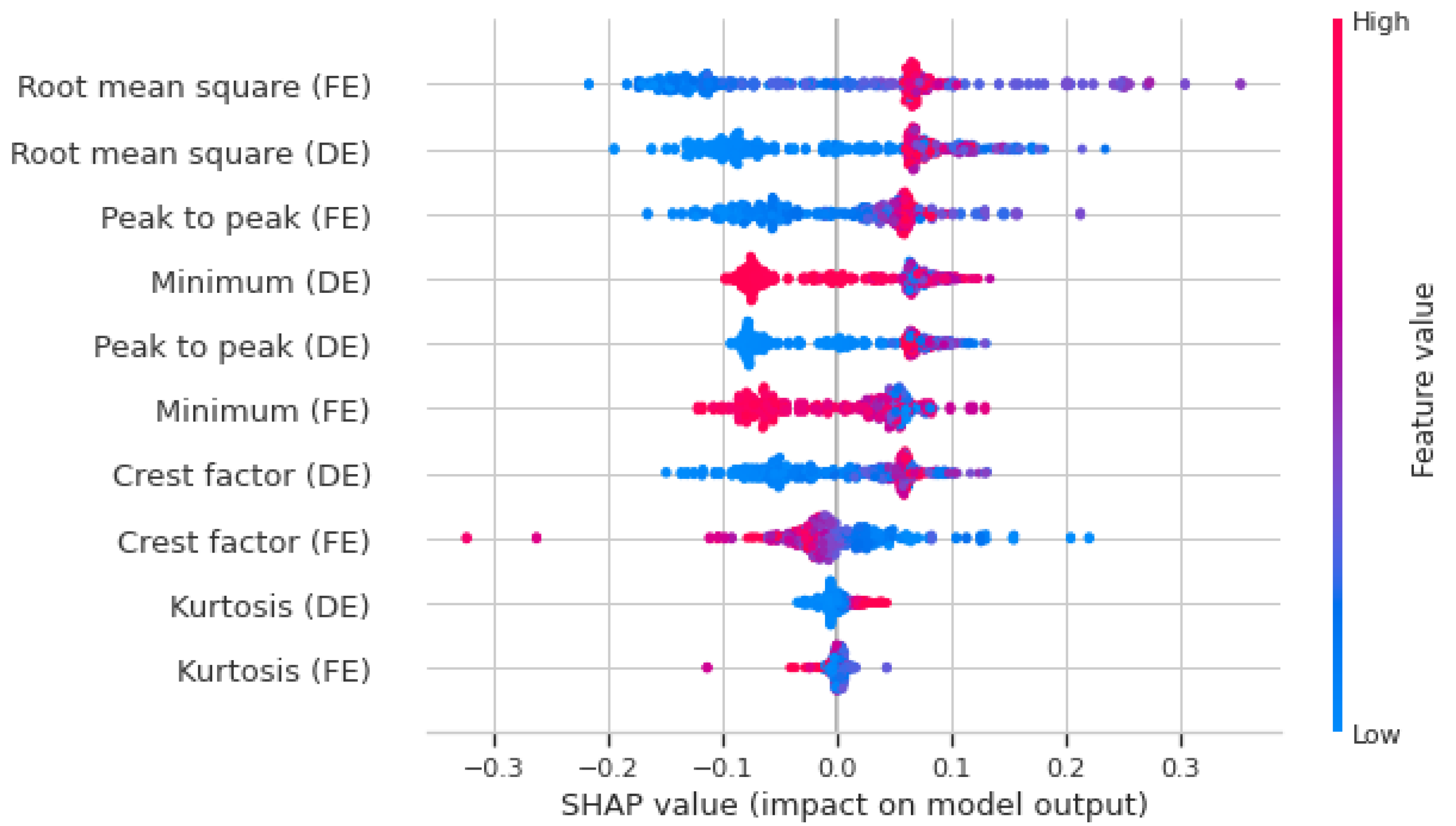
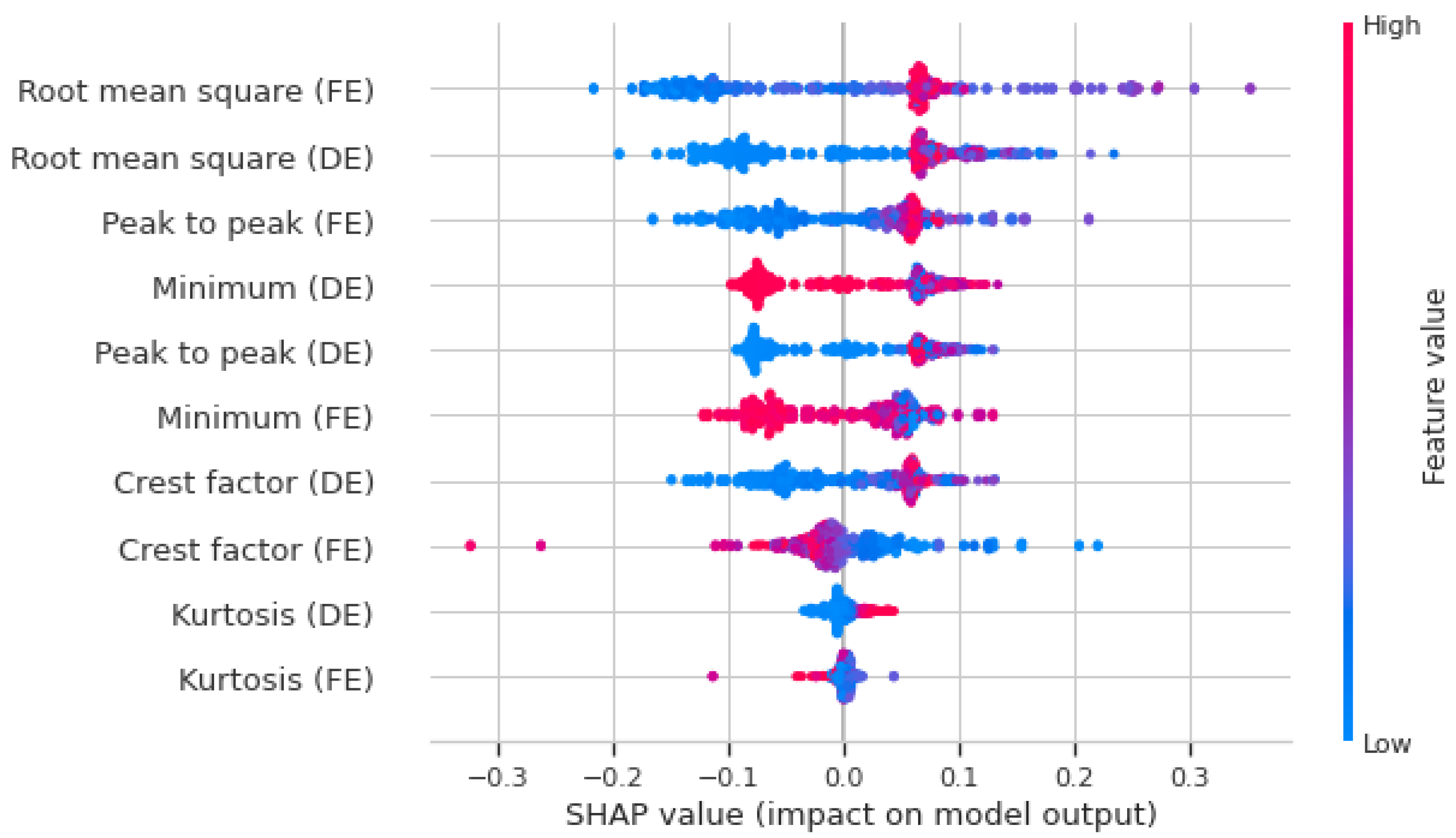
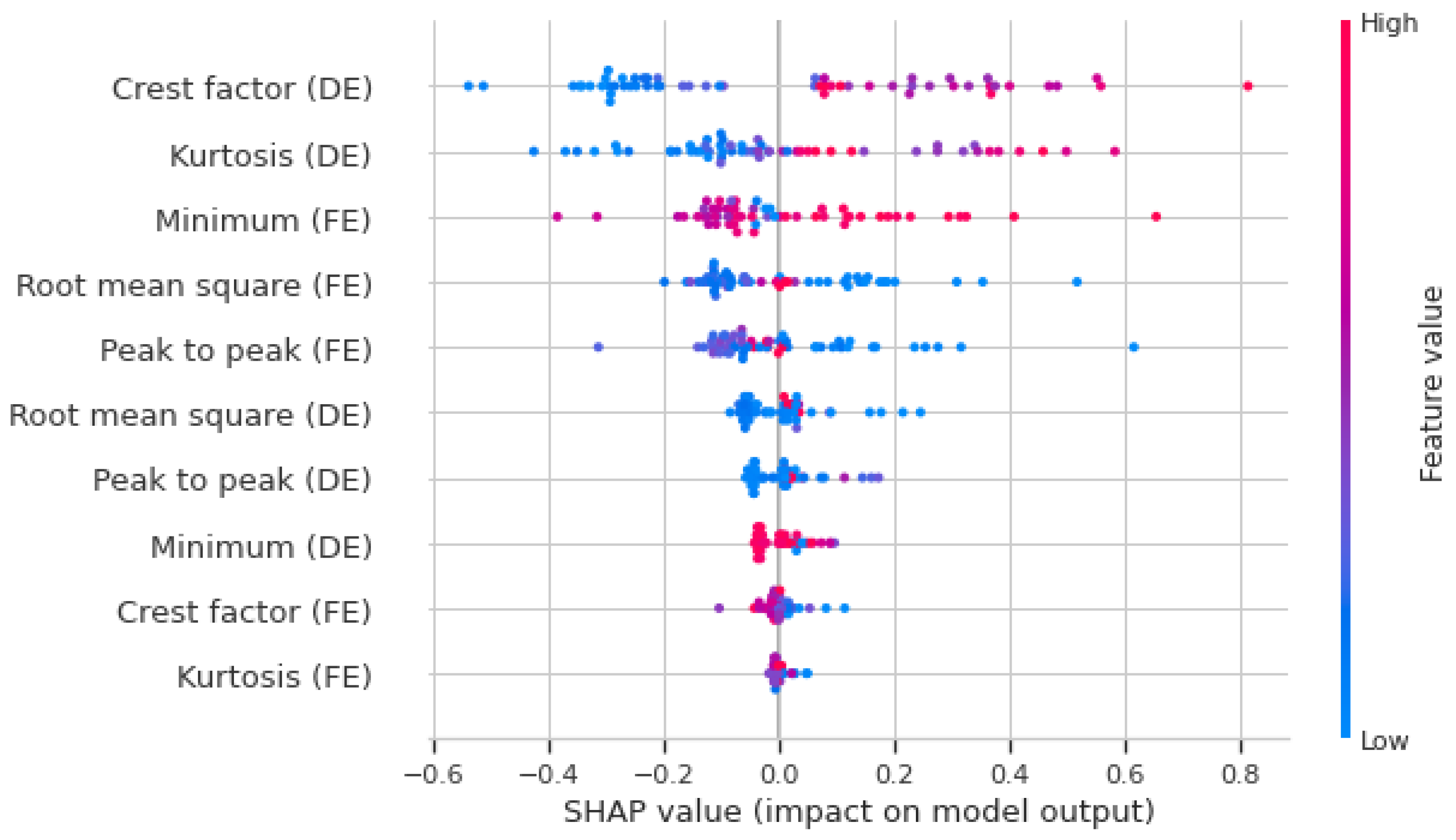
  • The vertical position identifies the corresponding feature.
  • The horizontal position indicates whether the value’s influence resulted in a higher or lower prediction.
  • The color represents whether the data’s value is categorized as high or low.
This analytical approach using the SHAP summary plot provides a visually intuitive and insightful means of understanding the individual feature contributions to the overall decision-making process of machine learning models.
Researchers and practitioners often leverage SHAP for tasks such as model debugging, feature importance analysis, and model comparison. Its application extends to various domains, including finance, healthcare, and natural language processing. As the field of XAI continues to evolve, SHAP remains a cornerstone in providing transparent and interpretable insights into the complex decision-making processes of machine learning models.

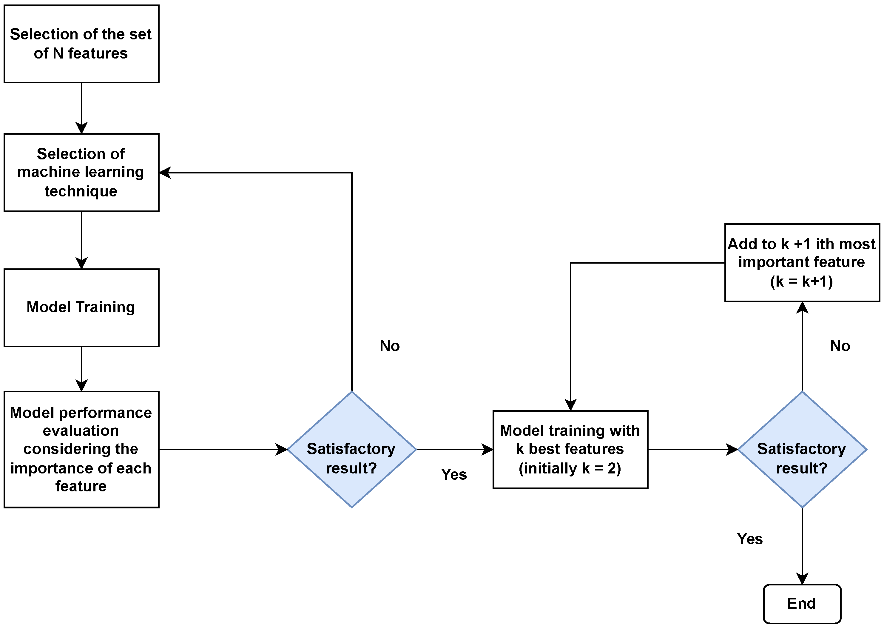
3. Proposed FDD Approach
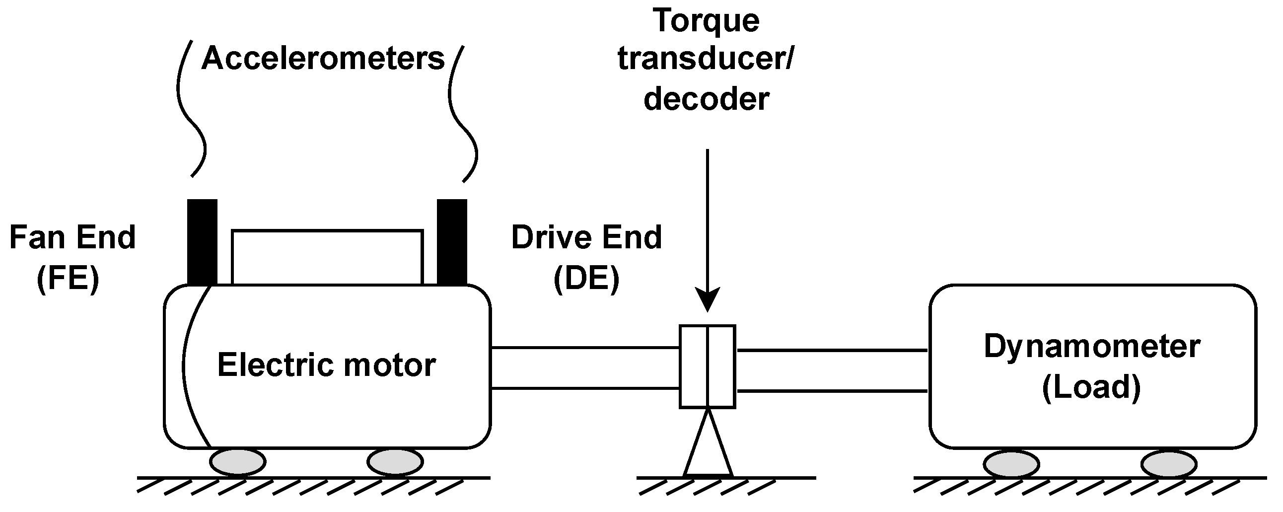
To achieve precise and efficient FDD models for the rolling bearing components in rotary machines, the approach is structured into three sequential phases: (1) fault detection, (2) fault classification, and (3) fault severity estimation.
In the fault detection phase, potential faults within the system are initially identified in the data. The fault classification phase exclusively employs the data identified as faulty from the initial phase, ensuring that the analysis is based solely on relevant fault-related information to enhance accuracy. Subsequently, in the fault severity estimation phase, data are systematically categorized based on the fault classes determined during the classification step. This targeted categorization allows for a meticulous examination of each fault class. This structured progression enables more precise and specialized severity estimations, building upon insights derived from prior classifications. The block diagram of the FDD proposal is shown in Figure 2.
Figure 3 illustrates the sequential progression of activities within each of the three phases of the proposal: fault detection, classification, and severity estimation. These activities encompass the extraction and selection of features, the choice of the ML technique, the complete training of the model, the comprehensive evaluation of the model’s performance, the subsequent training of a reduced model with the selected features, the assessment of the outcomes of the reduced model, and the potential inclusion of additional features if needed to enhance the model’s performance.
The literature offers numerous approaches for extracting features from vibration signals in rotary machines [10,66]. These features can be acquired through various techniques, including time domain methods involving statistical measures, frequency domain techniques encompassing coefficients of the fast Fourier transform (FFT), and time-frequency domain techniques involving coefficients of the discrete wavelet transform (DWT). In the validation of the proposal, statistical measures in the time domain of the vibration signals were exclusively employed. Specifically, peak to peak, root mean square, maximum, minimum, standard deviation, crest factor, and kurtosis values were selected as the features for the FDD model. These seven features were integrated into the full model training process. It is worth noting that prior to model development, exploratory data analysis (EDA) was conducted to assess the data, eliminating features exhibiting high auto-correlation. This process not only aids in refining the feature selection but also plays a crucial role in detecting any anomalies or inconsistencies within the dataset.
The subsequent activity involves the selection of an appropriate ML technique along with its pertinent hyper-parameters, all aimed at constructing a robust full model. For the purpose of validating the proposal, the exclusive adoption of the support vector machine (SVM) is made as the model for all three phases of the approach: fault detection, classification, and severity estimation. The next step involves the creation of meticulously trained ML-based models designed to achieve optimal performance. In this validation process, accuracy is selected as the performance metric, contributing to the evaluation of the proposal’s efficacy and accuracy.
Subsequently, once a satisfactory full model has been established, a pivotal activity involves assessing the significance of each individual feature in contributing to the model’s performance. To achieve this, the approach proposes the application of an explainable artificial intelligence (XAI) technique. In particular, this endeavor seeks to unveil the inner workings of the ML model, shedding light on how it discerns and processes data to detect, classify, and estimate the severity of faults. In this context, the Python package SHAP (Shapley additive explanations) has been utilized to systematically quantify and elucidate the role of each feature in shaping the performance of each full model.
Lastly, with the objective of attaining precise and efficient models, contingent on the significance of the chosen subset of features for model performance, a series of reduced models are evaluated iteratively until a satisfactory outcome is achieved.
To initiate this procedure, it begins by selecting the two most critical features that play a pivotal role in the decision-making mechanism of the fault detection and diagnosis (FDD) model. Subsequently, the FDD model undergoes exclusive training using these two chosen features as its input. If the obtained results are deemed unsatisfactory, the introduction of the third most relevant feature into the input of the fault detection model initiates the process anew. This iterative feature selection process continues until a predefined performance threshold is achieved. In this context, the accuracy metric is used as the designated criterion for determining the performance threshold.
It is crucial to emphasize that this approach is incredibly versatile, allowing for application across a wide range of datasets. Furthermore, it enables the extraction of various features and the utilization of diverse machine learning techniques, along with different feature selection approaches. In the context of this specific study, conducted with the purpose of validating the proposal, we chose to adopt the Case Western Reserve University (CWRU) benchmark [67].
The features calculated in the time domain were extensively explored, encompassing characteristics such as peak to peak, root mean square, maximum, minimum, standard deviation, crest factor, and kurtosis. These measurements were conducted for each sensor dataset available in this dataset, including a drive end (DE) accelerometer and a fan end (FE) accelerometer.
The chosen machine learning technique for this research was the support vector machine (SVM) with a linear kernel, providing robustness to the obtained results. Additionally, for feature selection based on importance, we employed the Python package SHAP (Shapley additive explanations), a reliable tool to elucidate the role and contribution of each feature to the model’s performance. This choice was based on the need to understand and highlight the factors that most influence model predictions, thereby contributing to the transparency and interpretability of the process.

4. Case Study

In order to validate the FDD approach proposed in this study, a comprehensive case study was conducted using data sourced from the widely recognized benchmark, Case Western Reserve University (CWRU) [67]. This benchmark involves a 1491.4 Watts electrical motor operating under normal conditions as well as bearing rolling fault scenarios. Bearing systems comprise essential components such as a torque sensor, decoder, dynamometer, eletric motor and two vibration sensors: a drive end (DE) accelerometer and a fan end (FE) accelerometer. Figure 4 shows the diagram of the infrastructure of the Case Western Reserve University benchmark.
For the experiments performed here, information from the two vibration sensors (FE and DE) sampled at 12,000 Hz for the electrical motor operating in 1797 revolutions per minute (RPM) was used. For these two sensors, the following time domain features were calculated: peak to peak, crest factor, root mean square, maximum, minimum, standard deviation, and kurtosis [10,33,34,35,36,37,38,39]. A non-overlapping one-second time window was employed to calculate the features used in all experiments.
The values presented in Table 1 provide a comprehensive overview of different fault types, along with their corresponding severity estimates, as part of a case study conducted using the CWRU. This dataset involves a two-horsepower electrical motor operating across various fault scenarios, including normal operation. Each fault type is assigned a unique identifier, denoted as “ F 0 ” to “ F 6 ”, and is associated with specific fault conditions. The “Fault Type” column ranges from “No Fault” to “Inner Race Fault”. The severity of each fault is quantified using diameter measurements in inches, providing essential insights into the extent of the fault’s impact. The “Fault Description” column offers succinct explanations of the fault types and their corresponding conditions.
Table 1 serves as a valuable reference to comprehend the fault types, their severity levels, and their associated explanations within the context of the presented case study. It aids in understanding the underlying fault scenarios and their varying effects on the system’s performance.
Figure 5 depicts a tree diagram illustrating the process of the proposed approach, utilizing the dataset provided earlier for the three-phase analysis:
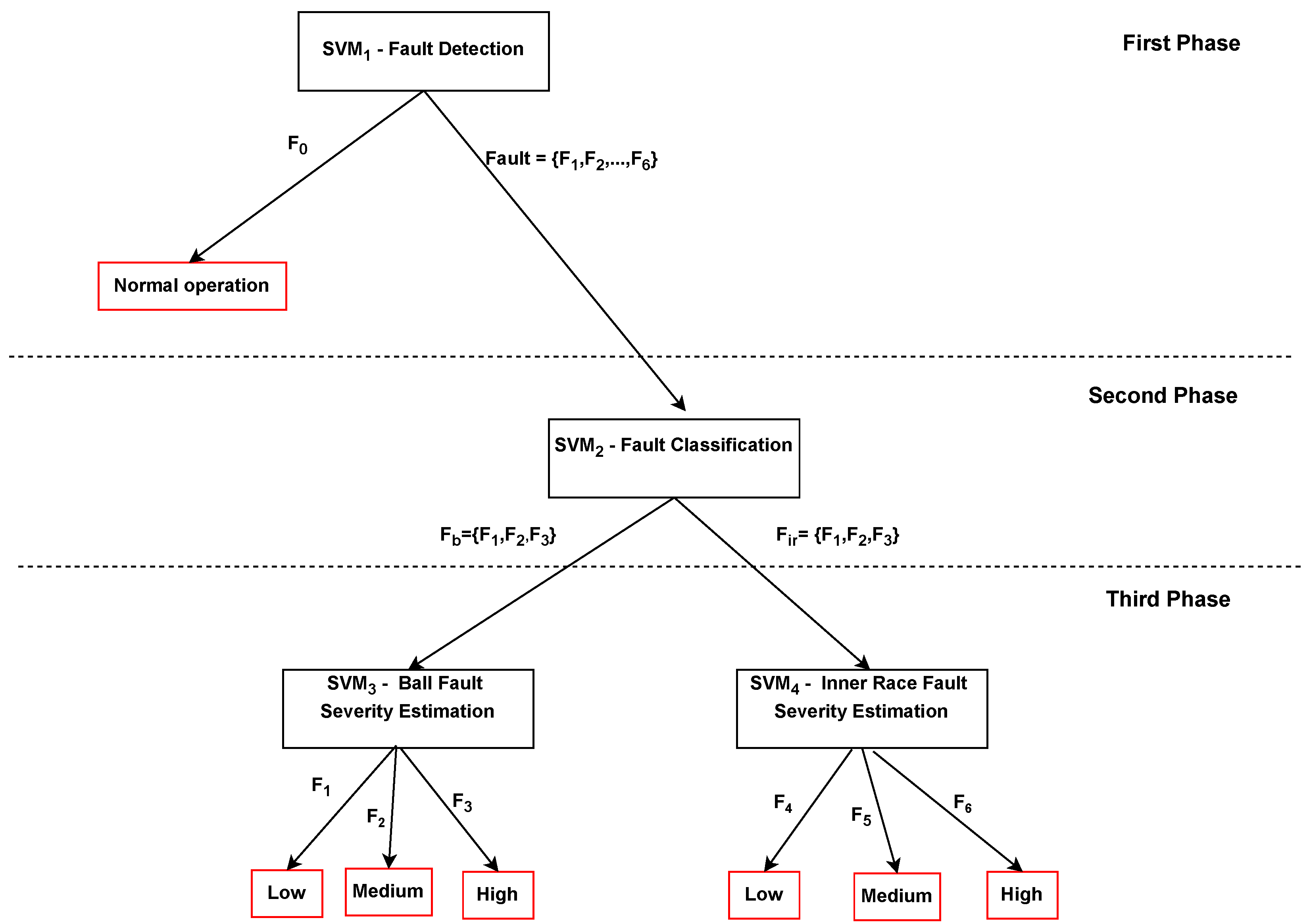
  • First phase (fault detection): In this initial phase, a support vector machine (SVM1) is employed to perform fault detection. The SVM1 model is trained to distinguish between normal operation ( F 0 ) and any form of fault ( F 1 , F 2 , , F 6 ). The SVM1 effectively separates the instances of normal operation from those associated with various fault conditions.
  • Second phase (fault classification): Building upon the results of the first phase, a second support vector machine (SVM2) is utilized for fault classification. This SVM2 model focuses on the specific fault types, particularly differentiating between Ball Faults ( F 1 , F 2 , F 3 ) and Inner Race Faults ( F 4 , F 5 , F 6 ). SVM2 discriminates instances belonging to Ball Faults and Inner Race Faults based on their unique characteristics.
  • Third phase (fault severity estimation): The final phase encompasses two sub-phases, each dedicated to severity estimation for distinct fault types. For Ball Faults, a dedicated support vector machine (SVM3) is employed. SVM3 classifies the severity of Ball Faults into three levels: low, medium, and high. Similarly, for Inner Race Faults, a separate support vector machine (SVM4) is used for severity estimation. SVM4 divides the Inner Race Faults into three severity categories: low, medium, and high.
In summary, this tree diagram visually represents the cascading sequence of activities across the three phases, demonstrating how the SVM models are strategically utilized to achieve fault detection, classification, and severity estimation in a systematic manner.
In the following subsections, the outcomes acquired for the fault detection, fault classification, and fault severity estimation phases are presented.

4.1. Fault Detection Phase

Figure 6 introduces a subset of the dataset utilized for training the fault detection model. This dataset encompasses distinct operational regions, each associated with a specific fault type: Normal Operation— F 0 , Inner Race Fault— F 4 , Ball Fault— F 1 , Inner Race Fault— F 6 , and Ball Fault— F 3 . Notably, this segment is marked by vertical dashed lines. In Figure 6a, the highlighted features stem from computations using drive end (DE) accelerometer sensor data: peak to peak (DE), crest factor (DE), and kurtosis (DE). Meanwhile, in Figure 6b, the features depicted arise from computations utilizing drive end (DE) sensor data: root mean square (DE), standard deviation (DE), maximum (DE), and minimum (DE). In Figure 6c, the highlighted features originate from computations using fan end (FE) accelerometer sensor data: peak to peak (FE), crest factor (FE), and kurtosis (FE). Conversely, in Figure 6d, the illustrated features emerge from computations utilizing fan end (FE) sensor data: root mean square (FE), standard deviation (FE), maximum (FE), and minimum (FE). The sequence employed in the training experiment is as follows: F 0 , F 4 , F 0 , F 1 , F 0 , F 6 , F 0 , F 3 , F 0 , as shown in Figure 6.
Figure 7 introduces a subset of the dataset utilized for testing the fault detection model. This dataset encompasses distinct operational regions, each associated with a specific fault type: Normal Operation— F 0 , Inner Race Fault— F 5 , Ball Fault— F 2 . These regions seamlessly integrate with the foundational Normal Operation— F 0 . Notably, this segment is marked by vertical dashed lines. In Figure 7a, the highlighted features stem from computations using drive end (DE) accelerometer sensor data: peak to peak (DE), crest factor (DE), and kurtosis (DE). Meanwhile, in Figure 7b, the features depicted arise from computations utilizing drive end (DE) sensor data: root mean square (DE), standard deviation (DE), maximum (DE), and minimum (DE). In Figure 7c, the highlighted features originate from computations using fan end (FE) accelerometer sensor data: peak to peak (FE), crest factor (FE), and kurtosis (FE). Conversely, in Figure 7d, the illustrated features emerge from computations utilizing fan end (FE) sensor data: root mean square (FE), standard deviation (FE), maximum (FE), and minimum (FE). The sequence employed in the training experiment is as follows: F 0 , F 5 , F 0 , F 2 , F 0 as shown in Figure 7.
To ensure the model’s impartiality, a two-step procedure was implemented. Initially, normalization of all features to a scale between 0 and 1 was carried out. Following this, a correlation matrix encompassing all the features was constructed, and a selection process for highly correlated features was applied. Specifically, when a group of features exhibited correlations of 95% or higher, only one feature from this group was retained. The features that surpassed this correlation threshold and were subsequently removed included: standard deviation (DE), standard deviation (FE), maximum (DE), and maximum (FE).
In this study, a support vector machine (SVM) with a linear kernel was employed as the machine learning model for fault detection. This SVM was trained using ten distinct features: peak to peak (DE), peak to peak (FE), root mean square (DE), root mean square (FE), crest factor (DE), crest factor (FE), minimum (DE), minimum (FE), kurtosis (DE), and kurtosis (FE). The model demonstrated a commendable performance, achieving an accuracy rate of 96%. This level of accuracy is considered highly satisfactory, considering that the predefined minimum acceptable threshold was set at 95%. This threshold was established based on a review of relevant literature employing similar techniques on the same dataset [19].
To gain deeper insights into the model’s decision-making process, the proposed approach outlined in Figure 3 was followed. Specifically, the SHAP (Shapley additive explanations) library was used to identify the most influential features in the fault detection model. The resulting graphical representation in Figure 8 displays these features in descending order of importance. Remarkably, it reveals that root mean square (FE) emerges as the most influential feature, while kurtosis (FE) has the least impact on the model’s decision-making process.
In the subsequent stage of the proposed approach, reduced fault detection models were evaluated. Features were incorporated into the model according to their importance ranking. This process commenced with a fault detection model using only the two most critical features (k = 2), specifically root mean square (FE) and root mean square (DE). Impressively, this reduced model achieved an accuracy of 97%. Given that this accuracy surpasses the predefined threshold of 95%, there was no need to introduce additional features to the fault detection model. Notably, it is essential to highlight that this reduced model outperformed the full model, which incorporated all ten features.
To gain a deeper understanding of how the number of features influences the fault detection model, models were evaluated using a range of two to ten features. The performance results are summarized in Table 2. Notably, the most favorable trade-off between performance and feature count was achieved with k = 2 . In this configuration, the model utilized the fewest number of features while achieving the highest accuracy.
Figure 9 depicts a scatterplot showcasing two pivotal features, root mean square (FE) and root mean square (DE), crucial for fault detection. These features were identified as highly significant in the SHAP library graph presented in Figure 8. Upon close examination of the graph, it becomes evident that utilizing only these two features allows for a clear demarcation between fault data and normal operation.

4.2. Fault Classification Phase

Figure 10 introduces a subset of the dataset utilized for training the fault classification model. This dataset encompasses distinct operational regions, each associated with a specific fault type: Inner Race Fault— F 4 , Ball Fault— F 1 , Inner Race Fault— F 6 , and Ball Fault— F 3 . In Figure 10a, the highlighted features stem from computations using drive end (DE) accelerometer sensor data: peak to peak (DE), crest factor (DE), and kurtosis (DE). Meanwhile, in Figure 10b, the features depicted arise from computations utilizing drive end (DE) sensor data: root mean square (DE), standard deviation (DE), maximum (DE), and minimum (DE). In Figure 10c, the highlighted features originate from computations using fan end (FE) accelerometer sensor data: peak to peak (FE), crest factor (FE), and kurtosis (FE). Conversely, in Figure 10d, the illustrated features emerge from computations utilizing fan end (FE) sensor data: root mean square (FE), standard deviation (FE), maximum (FE), and minimum (FE). The sequence employed in the training experiment is as follows: F 4 , F 1 , F 6 , F 3 as shown in Figure 10.
Figure 11 introduces a subset of the dataset that has been specifically chosen for evaluating the fault classification model. This dataset covers various operational scenarios, each linked to a particular type of fault, namely Inner Race Fault ( F 5 ) and Ball Fault ( F 2 ). It is important to note that this portion of the dataset is demarcated by vertical dashed lines within the figure.
In Figure 11a, the highlighted features are the result of computations performed using data from the drive end (DE) accelerometer sensor. These features include peak to peak (DE), crest factor (DE), and kurtosis (DE). In contrast, Figure 11b displays features that are derived from calculations using drive end (DE) sensor data, encompassing root mean square (DE), standard deviation (DE), maximum (DE), and minimum (DE).
Moving on to Figure 11c, the highlighted features are generated through computations involving data from the fan end (FE) accelerometer sensor, specifically peak to peak (FE), crest factor (FE), and kurtosis (FE). Conversely, Figure 11d showcases features obtained from calculations utilizing fan end (FE) sensor data, which include root mean square (FE), standard deviation (FE), maximum (FE), and minimum (FE).
The experimental training sequence followed the order of faults F 5 and F 2 , as visually represented in Figure 11.
A support vector machine (SVM) employing a linear kernel was employed for the fault classification model. This comprehensive model, incorporating ten features (k = 10), achieved an accuracy of 84%. It is worth noting that an accuracy threshold of 80% was established as the performance benchmark.
Subsequently, in accordance with the proposed methodology, the significance of these ten features was assessed utilizing SHAP (Shapley additive explanations) graphs. In Figure 12, the SHAP summary plot is presented, offering insight into the relevance of each feature with regard to fault classification. This analysis reveals that the two most pivotal features in this context are the root mean square (FE) and peak to peak (FE).
In an effort to gain a deeper insight into the influence of feature quantity on the fault classification model, models were assessed using different numbers of features, ranging from two to ten. The corresponding performance results are detailed in Table 3. Notably, the most favorable cost–benefit ratio was achieved when employing only two features, denoted as k = 2 . This minimal feature set not only reduced complexity but also yielded the highest level of accuracy in the classification process.
Figure 13 depicts a scatterplot showcasing two pivotal features, root mean square (FE) and peak to peak (FE), crucial for fault classification. These features were identified as highly significant in the SHAP library graph presented in Figure 12. Upon close examination of the graph, it becomes evident that utilizing only these two features allows for a clear demarcation between fault data and normal operation.

4.3. Fault Severity Estimation Phase

In this phase, the focus narrows down to two specific types of faults: Inner Race Faults and Ball Faults. For each of these fault types, three distinct levels of fault severity are meticulously examined: 0.1778 mm, 0.3556 mm, and 0.5334 mm.
Figure 14 presents a carefully curated subset of the dataset, specifically chosen for the purpose of fault severity estimation. This dataset comprises three distinct severities (fault diameters of 0.1778 mm, 0.3556 mm, and 0.5334 mm) for Inner Race Faults, designated as F 4 , F 5 , and F 6 , respectively. It is essential to emphasize that this portion of the dataset is visually delineated by vertical dashed lines within the figure.
In Figure 14a, the featured data derives from computations performed using data from the drive end (DE) accelerometer sensor. These featured parameters include peak to peak (DE), crest factor (DE), and kurtosis (DE). In contrast, Figure 14b showcases features calculated using drive end (DE) sensor data, encompassing root mean square (DE), standard deviation (DE), maximum (DE), and minimum (DE).
Moving on to Figure 14c, the highlighted features are the result of computations involving data from the fan end (FE) accelerometer sensor, specifically peak to peak (FE), crest factor (FE), and kurtosis (FE). Conversely, Figure 14d displays features obtained from calculations utilizing fan end (FE) sensor data, which include root mean square (FE), standard deviation (FE), maximum (FE), and minimum (FE).
Figure 15 showcases a carefully curated subset of the dataset, customized for precise fault severity estimation in Ball Faults. This dataset encompasses three different severity levels with fault diameters of 0.1778 mm, 0.3556 mm, and 0.5334 mm, denoted as F 1 , F 2 , and F 3 , respectively. It is crucial to highlight that this section of the dataset is visually delineated by vertical dashed lines within the figure.
In Figure 15a, the data featured here are the outcome of calculations performed using information from the drive end (DE) accelerometer sensor. These featured parameters encompass peak to peak (DE), crest factor (DE), and kurtosis (DE). Conversely, Figure 15b showcases features computed from drive end (DE) sensor data, including root mean square (DE), standard deviation (DE), maximum (DE), and minimum (DE).
Transitioning to Figure 15c, the highlighted features result from computations utilizing data from the fan end (FE) accelerometer sensor, specifically peak to peak (FE), crest factor (FE), and kurtosis (FE). In contrast, Figure 15d displays features derived from calculations using fan end (FE) sensor data, encompassing root mean square (FE), standard deviation (FE), maximum (FE), and minimum (FE).
The fault severity datasets were partitioned into a training set comprising 80% of the data and a testing set comprising the remaining 20%. The default training/test split ratio of 80%/20% was utilized, which is standard practice, particularly for larger datasets [68]. In this context, the dataset is deemed to be approximately balanced, as it encompasses fault data with comparable sample numbers. It is worth noting that the stratification strategy for the target classes defaulted to the settings provided by the Scikit-learn library, ensuring a systematic and reliable approach to maintain class distribution integrity during the split process [69]. The fault severity estimation model for both the “Inner Race” and “Ball” validation scenarios employed support vector machines (SVM) with a linear kernel.
The comprehensive Inner Race Fault severity model, featuring ten essential features (k = 10), achieved an impressive accuracy rate of 88%. Notably, a performance threshold of 85% was set as the benchmark for accuracy. Subsequently, following the proposed approach, the significance of these ten features was assessed using SHAP graphs.
Figure 16 showcases the SHAP summary plot, providing insights into the relevance of each feature concerning Inner Race Fault severity estimation. This analysis reveals that the two most influential features are the root mean square (DE) and peak to peak (DE).
In the pursuit of a deeper understanding of how the quantity of features affects the Inner Race Fault severity estimation model, evaluations were conducted using models comprising two to ten features. The model performances are summarized in Table 4. Notably, a significant improvement was observed with k = 2, where the model utilized the fewest features yet achieved commendable accuracy.
Figure 17 displays a scatterplot that highlights two critical features, peak to peak (DE) and root mean square (DE), which were identified as highly influential in the SHAP library graph presented in Figure 16. Upon close examination of the graph, it becomes evident that utilizing only these two features allows for a clear distinction between the three levels of severity.
The complete Ball Fault severity model, utilizing ten features (k = 10), achieved an accuracy rate of 75%. It is worth noting that a performance threshold of 75% was established for assessment. Subsequently, adhering to the proposed approach, the significance of these ten features was assessed through SHAP graphs.
Figure 18 presents the SHAP summary plot, which visually illustrates the relevance of each feature in estimating Ball Fault severity.
Following the proposed approach, the initial step involved selecting the two most relevant features for the Ball Fault severity model (k = 2), which turned out to be the crest factor (DE) and kurtosis (DE). However, upon analyzing the metrics, it became evident that the obtained result did not meet the set satisfaction criteria, as the accuracy fell below the acceptable threshold.
The process was then continued until a result surpassing the 75% accuracy threshold was achieved, which happened with a set of four features (k = 4). Table 5 presents the results obtained for Ball Fault severity estimation models using two to ten features. Notably, the best cost–benefit trade-off was observed with k = 4, where the highest accuracy was attained with a relatively small number of features.
Figure 19 exhibits a pairplot that effectively highlights four critical features: crest factor (DE), kurtosis (DE), minimum (FE), and root mean square (FE). This pairplot not only showcases the individual distributions of these features but also provides a comprehensive visualization of the relationships between them, offering valuable insights into their bivariate interactions. These features, identified as highly influential in the SHAP library graph presented in Figure 18, play a crucial role in understanding the underlying patterns in the data.
Upon a meticulous examination of the pairplot, it becomes evident that relying solely on these four features does not yield a clear distinction between the three levels of severity. This observation underscores the complexity of the relationships and the importance of considering additional features or refining the feature selection process for a more nuanced understanding of the severity levels.

5. Conclusions

The scientific justification for the research presented in this paper lies in the development of a groundbreaking methodology aimed at enhancing fault detection, classification, and severity estimation in rolling element bearings. The unique approach comprises three sequential phases, each dedicated to constructing distinct machine-learning-based models to address essential tasks. The methodology stands out for its ability to leverage information obtained in one phase to optimize subsequent phases, thereby improving overall Fault diagnosis effectiveness.
At the core of the approach is the integration of explainable artificial intelligence (XAI) techniques, which facilitate the meticulous selection of optimal features for machine learning models. The chosen machine learning technique for these tasks is the support vector machine (SVM), recognized for its robustness and versatility.
To rigorously validate the approach, the widely recognized Case Western Reserve University benchmark, a gold standard in bearing fault analysis, was employed. Even when working with a highly limited number of features, the models consistently attained evaluation metrics with an accuracy exceeding 90% in the majority of cases.
In summary, this study represents a significant advancement in the field of fault detection and classification in rolling element bearings. The novel approach not only produces efficient and accurate fault models but also offers interpretability through XAI techniques. By providing insights into the rationale behind feature selection, the approach empowers decision-makers in the design of fault models, making it a valuable asset in various industrial scenarios. These findings emphasize the effectiveness and interpretability of the approach and open up new possibilities for enhancing the reliability and maintenance of critical machinery.

Author Contributions

Conceptualization, M.R.S.; Methodology, M.R.S. and A.G.; Software, M.R.S. and A.G.; Validation, M.R.S., A.G. and I.S.-G.; Investigation, M.R.S., A.G. and I.S.-G.; Writing, M.R.S., A.G. and I.S.-G.; Writing—review, M.R.S., A.G. and I.S.-G. All authors have read and agreed to the published version of the manuscript.

Funding

Coordenação de Aperfeicoamento de Pessoal de Nível Superior.

Data Availability Statement

Data is contained within the article.

Conflicts of Interest

The authors declare no conflict of interest.

References

  1. Mikić, D.; Desnica, E.; Ašonja, A.; Stojanovic, B.; Epifanić-Pajić, V. Reliability Analysis of Ball Bearing on the Crankshaft of Piston Compressors. J. Balk. Tribol. Assoc. 2016, 22, 5060–5070. [Google Scholar]
  2. Randall, R.B.; Antoni, J. Rolling element bearing diagnostics—A tutorial. Mech. Syst. Signal Process. 2011, 25, 485–520. [Google Scholar] [CrossRef]
  3. Desnica, E.; Ašonja, A.; Radovanović, L.; Palinkaš, I.; Kiss, I. Selection, Dimensioning and Maintenance of Roller Bearings. In Proceedings of the 31st International Conference on Organization and Technology of Maintenance (OTO 2022), Osijek, Croatia, 12 December 2022; Blažević, D., Ademović, N., Barić, T., Cumin, J., Desnica, E., Eds.; Springer: Cham, Switzerland, 2023; pp. 133–142. [Google Scholar]
  4. Santos, M.R.; Affonso Guedes, L. An Evolving Approach to Fault Detection of Rolling Element Bearings. In Proceedings of the 2021 International Conference on Control, Automation and Diagnosis (ICCAD), Grenoble, France, 3–5 November 2021; pp. 1–5. [Google Scholar] [CrossRef]
  5. Sharma, A.; Patra, G.K.; Naidu, V. Bearing Fault Classification using Acoustic Features and Artificial Neural Network. In Proceedings of the 2022 4th International Conference on Circuits, Control, Communication and Computing (I4C), Bangalore, India, 21–23 December 2022; pp. 421–425. [Google Scholar] [CrossRef]
  6. Pastukhov, A.; Timashov, E.; Stanojević, D. Temperature Conditions and Diagnostics of Bearings. Appl. Eng. Lett. J. Eng. Appl. Sci. 2023, 8, 45–51. [Google Scholar] [CrossRef]
  7. Wakiru, J.; Pintelon, L.; Muchiri, P.; Chemweno, P. A data mining approach for lubricant-based fault diagnosis. J. Qual. Maint. Eng. 2020, 27, 264–291. [Google Scholar] [CrossRef]
  8. Cerrada, M.; Sánchez, R.V.; Li, C.; Pacheco, F.; Cabrera, D.; Valente de Oliveira, J.; Vásquez, R.E. A review on data-driven fault severity assessment in rolling bearings. Mech. Syst. Signal Process. 2018, 99, 169–196. [Google Scholar] [CrossRef]
  9. Nelson, W.; Culp, C. FDD in Building Systems Based on Generalized Machine Learning Approaches. Energies 2023, 16, 1637. [Google Scholar] [CrossRef]
  10. Mohamad, T.H.; Nataraj, C. Fault identification and severity analysis of rolling element bearings using phase space topology. J. Vib. Control 2021, 27, 295–310. [Google Scholar] [CrossRef]
  11. Lei, Y.; Yang, B.; Jiang, X.; Jia, F.; Li, N.; Nandi, A.K. Applications of machine learning to machine fault diagnosis: A review and roadmap. Mech. Syst. Signal Process. 2020, 138, 106587. [Google Scholar] [CrossRef]
  12. Shenfield, A.; Howarth, M. A Novel Deep Learning Model for the Detection and Identification of Rolling Element-Bearing Faults. Sensors 2020, 20, 5112. [Google Scholar] [CrossRef]
  13. Han, H.; Gu, B.; Wang, T.; Li, Z. Important sensors for chiller fault detection and diagnosis (FDD) from the perspective of feature selection and machine learning. Int. J. Refrig. 2011, 34, 586–599. [Google Scholar] [CrossRef]
  14. Kim, M.Y.; Atakishiyev, S.; Babiker, H.K.B.; Farruque, N.; Goebel, R.; Zaïane, O.R.; Motallebi, M.H.; Rabelo, J.; Syed, T.; Yao, H.; et al. A Multi-Component Framework for the Analysis and Design of Explainable Artificial Intelligence. Mach. Learn. Knowl. Extr. 2021, 3, 900–921. [Google Scholar] [CrossRef]
  15. Hulsen, T. Explainable Artificial Intelligence (XAI): Concepts and Challenges in Healthcare. AI 2023, 4, 652–666. [Google Scholar] [CrossRef]
  16. Ghnemat, R.; Alodibat, S.; Abu Al-Haija, Q. Explainable Artificial Intelligence (XAI) for Deep Learning Based Medical Imaging Classification. J. Imaging 2023, 9, 177. [Google Scholar] [CrossRef]
  17. Clement, T.; Kemmerzell, N.; Abdelaal, M.; Amberg, M. XAIR: A Systematic Metareview of Explainable AI (XAI) Aligned to the Software Development Process. Mach. Learn. Knowl. Extr. 2023, 5, 78–108. [Google Scholar] [CrossRef]
  18. Lundberg, S.M.; Lee, S.I. A Unified Approach to Interpreting Model Predictions. In Advances in Neural Information Processing Systems 30; Guyon, I., Luxburg, U.V., Bengio, S., Wallach, H., Fergus, R., Vishwanathan, S., Garnett, R., Eds.; Curran Associates, Inc.: Red Hook, NY, USA, 2017; pp. 4765–4774. [Google Scholar]
  19. Smith, W.A.; Randall, R.B. Rolling element bearing diagnostics using the Case Western Reserve University data: A benchmark study. Mech. Syst. Signal Process. 2015, 64–65, 100–131. [Google Scholar] [CrossRef]
  20. Bezerra, C.G.; Costa, B.S.J.; Guedes, L.A.; Angelov, P.P. An evolving approach to unsupervised and Real-Time fault detection in industrial processes. Expert Syst. Appl. 2016, 63, 134–144. [Google Scholar] [CrossRef]
  21. Venkatasubramanian, V.; Rengaswamy, R.; Yin, K.; Kavuri, S.N. A review of process fault detection and diagnosis: Part I: Quantitative model-based methods. Comput. Chem. Eng. 2003, 27, 293–311. [Google Scholar] [CrossRef]
  22. Wang, P.; Guo, C. Based on the coal mine’s essential safety management system of safety accident cause analysis. Am. J. Environ. Energy Power Res. 2013, 1, 62–68. [Google Scholar]
  23. Li, Z.; Wang, Y.; Wang, K.S. Intelligent predictive maintenance for fault diagnosis and prognosis in machine centers: Industry 4.0 scenario. Adv. Manuf. 2017, 5, 377–387. [Google Scholar] [CrossRef]
  24. Del Buono, F.; Calabrese, F.; Baraldi, A.; Paganelli, M.; Guerra, F. Novelty Detection with Autoencoders for System Health Monitoring in Industrial Environments. Appl. Sci. 2022, 12, 4931. [Google Scholar] [CrossRef]
  25. Jalayer, M.; Kaboli, A.; Orsenigo, C.; Vercellis, C. Fault Detection and Diagnosis with Imbalanced and Noisy Data: A Hybrid Framework for Rotating Machinery. Machines 2022, 10, 237. [Google Scholar] [CrossRef]
  26. Yin, L.; Wang, H.; Fan, W.; Kou, L.; Lin, T.; Xiao, Y. Incorporate active learning to semi-supervised industrial fault classification. J. Process Control 2019, 78, 88–97. [Google Scholar] [CrossRef]
  27. Sorsa, T.; Koivo, H.N.; Koivisto, H. Neural networks in process fault diagnosis. IEEE Trans. Syst. Man, Cybern. 1991, 21, 815–825. [Google Scholar] [CrossRef]
  28. Ayoubi, M. Nonlinear dynamic systems identification with dynamic neural networks for fault diagnosis in technical processes. In Proceedings of the IEEE International Conference on Systems, Man and Cybernetics, San Antonio, TX, USA, 2–5 October 1994; Volume 3, pp. 2120–2125. [Google Scholar]
  29. Khan, S.; Yairi, T. A review on the application of deep learning in system health management. Mech. Syst. Signal Process. 2018, 107, 241–265. [Google Scholar] [CrossRef]
  30. Liu, R.; Yang, B.; Zio, E.; Chen, X. Artificial intelligence for fault diagnosis of rotating machinery: A review. Mech. Syst. Signal Process. 2018, 108, 33–47. [Google Scholar] [CrossRef]
  31. Khalid, S.; Khalil, T.; Nasreen, S. A survey of feature selection and feature extraction techniques in machine learning. In Proceedings of the 2014 Science and Information Conference, London, UK, 27–29 August 2014; pp. 372–378. [Google Scholar] [CrossRef]
  32. Ganesh, S.; Beucler, T.; Tam, F.; Gomez, M.; Runge, J.; Gerhardus, A. Selecting robust features for machine-learning applications using multidata causal discovery. Environ. Data Sci. 2023, 2, e27. [Google Scholar] [CrossRef]
  33. Du, S.C.; Liu, T.; Huang, D.L.; Li, G.L. An Optimal Ensemble Empirical Mode Decomposition Method for Vibration Signal Decomposition. J. Vib. Acoust. 2017, 139, 031003. [Google Scholar] [CrossRef]
  34. Sreejith, B.; Verma, A.; Srividya, A. Fault diagnosis of rolling element bearing using time domain features and neural networks. In Proceedings of the 2008 IEEE Region 10 and the Third international Conference on Industrial and Information Systems, Kharagpur, India, 8–10 December 2008; pp. 1–6. [Google Scholar] [CrossRef]
  35. Yiakopoulos, C.; Gryllias, K.; Antoniadis, I. Rolling element bearing fault detection in industrial environments based on a K-means clustering approach. Expert Syst. Appl. 2011, 38, 2888–2911. [Google Scholar] [CrossRef]
  36. Dhamande, L.S.; Chaudhari, M.B. Compound gear-bearing fault feature extraction using statistical features based on time-frequency method. Measurement 2018, 125, 63–77. [Google Scholar] [CrossRef]
  37. Grover, C.; Turk, N. Optimal Statistical Feature Subset Selection for Bearing Fault Detection and Severity Estimation. Shock Vib. 2020, 2020, 5742053. [Google Scholar] [CrossRef]
  38. Nayana, B.R.; Geethanjali, P. Analysis of Statistical Time-Domain Features Effectiveness in Identification of Bearing Faults from Vibration Signal. IEEE Sens. J. 2017, 17, 5618–5625. [Google Scholar] [CrossRef]
  39. Zhan, L.; Ma, F.; Zhang, J.; Li, C.; Li, Z.; Wang, T. Fault Feature Extraction and Diagnosis of Rolling Bearings Based on Enhanced Complementary Empirical Mode Decomposition with Adaptive Noise and Statistical Time-Domain Features. Sensors 2019, 19, 4047. [Google Scholar] [CrossRef] [PubMed]
  40. Seryasat, O.; Aliyari shoorehdeli, M.; Honarvar, F.; Rahmani, A. Multi-fault diagnosis of Ball bearing using FFT, wavelet energy entropy mean and root mean square (RMS). In Proceedings of the 2010 IEEE International Conference on Systems, Man and Cybernetics, Istanbul, Turkey, 10–13 October 2010; pp. 4295–4299. [Google Scholar] [CrossRef]
  41. Xiang, C.; Ren, Z.; Shi, P.; Zhao, H. Data-Driven Fault Diagnosis for Rolling Bearing Based on DIT-FFT and XGBoost. Complexity 2021, 2021, 4941966. [Google Scholar] [CrossRef]
  42. Cocconcelli, M.; Zimroz, R.; Rubini, R.; Bartelmus, W. STFT Based Approach for Ball Bearing Fault Detection in a Varying Speed Motor. In Condition Monitoring of Machinery in Non-Stationary Operations; Springer: Berlin/Heidelberg, Germany, 2012. [Google Scholar]
  43. Gao, H.; Liang, L.; Chen, X.; Xu, G. Feature extraction and recognition for rolling element bearing fault utilizing short-time Fourier transform and non-negative matrix factorization. Chin. J. Mech. Eng. 2014, 28, 96–105. [Google Scholar] [CrossRef]
  44. Tao, H.; Wang, P.; Chen, Y.; Stojanovic, V.; Yang, H. An unsupervised fault diagnosis method for rolling bearing using STFT and generative neural networks. J. Frankl. Inst. 2020, 357, 7286–7307. [Google Scholar] [CrossRef]
  45. Kankar, P.; Sharma, S.C.; Harsha, S. Rolling element bearing fault diagnosis using autocorrelation and continuous wavelet transform. J. Vib. Control 2011, 17, 2081–2094. [Google Scholar] [CrossRef]
  46. Kankar, P.; Sharma, S.C.; Harsha, S. Rolling element bearing fault diagnosis using wavelet transform. Neurocomputing 2011, 74, 1638–1645. [Google Scholar] [CrossRef]
  47. Konar, P.; Chattopadhyay, P. Bearing fault detection of induction motor using wavelet and Support Vector Machines (SVMs). Appl. Soft Comput. 2011, 11, 4203–4211. [Google Scholar] [CrossRef]
  48. Patil, A.B.; Gaikwad, J.A.; Kulkarni, J.V. Bearing fault diagnosis using discrete Wavelet Transform and Artificial Neural Network. In Proceedings of the 2016 2nd International Conference on Applied and Theoretical Computing and Communication Technology (iCATccT), Bangalore, India, 21–23 July 2016; pp. 399–405. [Google Scholar] [CrossRef]
  49. Yang, D.M. The Detection of Motor Bearing Fault with Maximal Overlap Discrete Wavelet Packet Transform and Teager Energy Adaptive Spectral kurtosis. Sensors 2021, 21, 6895. [Google Scholar] [CrossRef]
  50. Anbu, S.; Thangavelu, A.; Ashok, S.D. Fuzzy C-Means Based Clustering and Rule Formation Approach for Classification of Bearing Faults Using Discrete Wavelet Transform. Computation 2019, 7, 54. [Google Scholar] [CrossRef]
  51. Liang, L.; Shan, L.; Liu, F.; Niu, B.; Xu, G. Sparse Envelope Spectra for Feature Extraction of Bearing Faults Based on NMF. Appl. Sci. 2019, 9, 755. [Google Scholar] [CrossRef]
  52. Liu, Y.; Qian, Q.; Liu, F.; Lu, S.; He, Q.; Zhao, J. Wayside Bearing Fault Diagnosis Based on Envelope Analysis Paved with Time-Domain Interpolation Resampling and Weighted-Correlation-Coefficient-Guided Stochastic Resonance. Shock Vib. 2017, 2017, 3189135. [Google Scholar] [CrossRef]
  53. Leite, V.C.M.N.; Borges da Silva, J.G.; Veloso, G.F.C.; Borges da Silva, L.E.; Lambert-Torres, G.; Bonaldi, E.L.; de Lacerda de Oliveira, L.E. Detection of Localized Bearing Faults in Induction Machines by Spectral kurtosis and Envelope Analysis of Stator Current. IEEE Trans. Ind. Electron. 2015, 62, 1855–1865. [Google Scholar] [CrossRef]
  54. Ben Ali, J.; Fnaiech, N.; Saidi, L.; Chebel-Morello, B.; Fnaiech, F. Application of empirical mode decomposition and artificial neural network for automatic bearing fault diagnosis based on vibration signals. Appl. Acoust. 2015, 89, 16–27. [Google Scholar] [CrossRef]
  55. Zhang, X.; Liang, Y.; Zhou, J.; Zang, Y. A novel bearing fault diagnosis model integrated permutation entropy, ensemble empirical mode decomposition and optimized SVM. Measurement 2015, 69, 164–179. [Google Scholar] [CrossRef]
  56. Mohanty, S.; Gupta, K.K.; Raju, K.S. Adaptive fault identification of bearing using empirical mode decomposition–principal component analysis-based average kurtosis technique. IET Sci. Meas. Technol. 2017, 11, 30–40. [Google Scholar] [CrossRef]
  57. Nishat Toma, R.; Kim, C.H.; Kim, J.M. Bearing Fault Classification Using Ensemble Empirical Mode Decomposition and Convolutional Neural Network. Electronics 2021, 10, 1248. [Google Scholar] [CrossRef]
  58. Peres, F.A.P.; Fogliatto, F.S. Variable selection methods in multivariate statistical process control: A systematic literature review. Comput. Ind. Eng. 2018, 115, 603–619. [Google Scholar] [CrossRef]
  59. Jović, A.; Brkić, K.; Bogunović, N. A review of feature selection methods with applications. In Proceedings of the 2015 38th International Convention on Information and Communication Technology, Electronics and Microelectronics (MIPRO), Opatija, Croatia, 25–29 May 2015; pp. 1200–1205. [Google Scholar] [CrossRef]
  60. Ali, S.; Abuhmed, T.; El-Sappagh, S.; Muhammad, K.; Alonso-Moral, J.M.; Confalonieri, R.; Guidotti, R.; Del Ser, J.; Díaz-Rodríguez, N.; Herrera, F. Explainable Artificial Intelligence (XAI): What we know and what is left to attain Trustworthy Artificial Intelligence. Inf. Fusion 2023, 99, 101805. [Google Scholar] [CrossRef]
  61. Machlev, R.; Heistrene, L.; Perl, M.; Levy, K.; Belikov, J.; Mannor, S.; Levron, Y. Explainable Artificial Intelligence (XAI) techniques for energy and power systems: Review, challenges and opportunities. Energy AI 2022, 9, 100169. [Google Scholar] [CrossRef]
  62. Longo, L.; Brcic, M.; Cabitza, F.; Choi, J.; Confalonieri, R.; Del Ser, J.; Guidotti, R.; Hayashi, Y.; Herrera, F.; Holzinger, A.; et al. Explainable Artificial Intelligence (XAI) 2.0: A Manifesto of Open Challenges and Interdisciplinary Research Directions. arXiv 2023, arXiv:2310.19775. [Google Scholar]
  63. Adadi, A.; Berrada, M. Peeking Inside the Black-Box: A Survey on Explainable Artificial Intelligence (XAI). IEEE Access 2018, 6, 52138–52160. [Google Scholar] [CrossRef]
  64. Rodríguez-Pérez, R.; Bajorath, J. Interpretation of Compound Activity Predictions from Complex Machine Learning Models Using Local Approximations and Shapley Values. J. Med. Chem. 2019, 63, 8761–8777. [Google Scholar] [CrossRef] [PubMed]
  65. Lundberg, S.M.; Erion, G.; Chen, H.; DeGrave, A.; Prutkin, J.M.; Nair, B.; Katz, R.; Himmelfarb, J.; Bansal, N.; Lee, S.I. From local explanations to global understanding with explainable AI for trees. Nat. Mach. Intell. 2020, 2, 2522–5839. [Google Scholar] [CrossRef] [PubMed]
  66. Delgado, M.; Cirrincione, G.; García, A.; Ortega, J.A.; Henao, H. Accurate bearing faults classification based on statistical-time features, curvilinear component analysis and neural networks. In Proceedings of the IECON 2012—38th Annual Conference on IEEE Industrial Electronics Society, Montreal, QC, Canada, 25–28 October 2012; pp. 3854–3861. [Google Scholar] [CrossRef]
  67. Neupane, D.; Seok, J. Bearing Fault Detection and Diagnosis Using Case Western Reserve University Dataset with Deep Learning Approaches: A Review. IEEE Access 2020, 8, 93155–93178. [Google Scholar] [CrossRef]
  68. Rácz, A.; Bajusz, D.; Héberger, K. Effect of Dataset Size and Train/Test Split Ratios in QSAR/QSPR Multiclass Classification. Molecules 2021, 26, 1111. [Google Scholar] [CrossRef]
  69. Pedregosa, F.; Varoquaux, G.; Gramfort, A.; Michel, V.; Thirion, B.; Grisel, O.; Blondel, M.; Prettenhofer, P.; Weiss, R.; Dubourg, V.; et al. Scikit-learn: Machine Learning in Python. J. Mach. Learn. Res. 2011, 12, 2825–2830. [Google Scholar]
Figure 1. Example of summary plot.
Make 06 00016 g001
Figure 2. Descriptive block diagram of the proposed FDD approach.
Make 06 00016 g002
Figure 3. Descriptive block diagram of the proposed FDD approach.
Make 06 00016 g003
Figure 4. Infrastructure of the Case Western Reserve University benchmark.
Make 06 00016 g004
Figure 5. Illustration of the three-phase approach for fault detection, classification, and severity estimation using SVM models. The tree diagram outlines the sequential progression of activities in each phase, showcasing the strategic application of support vector machine (SVM) models for efficient fault detection, classification, and severity estimation.
Make 06 00016 g005
Figure 6. Overview of the training dataset for the fault detection model: (a) Features computed from drive end (DE) accelerometer sensor data: peak to peak (DE), crest factor (DE), and kurtosis (DE). (b) Features computed using drive end (DE) sensor data: root mean square (DE), standard deviation (DE), maximum (DE), and minimum (DE). (c) Features originating from fan end (FE) accelerometer sensor data: peak to peak (FE), crest factor (FE), and kurtosis (FE). (d) Features computed using fan end (FE) sensor data: root mean square (FE), standard deviation (FE), maximum (FE), and minimum (FE).
Make 06 00016 g006
Figure 7. Overview of testing dataset for fault detection model: (a) Features computed from drive end (DE) accelerometer sensor data: peak to peak (DE), crest factor (DE), and kurtosis (DE). (b) Features computed using drive end (DE) sensor data: root mean square (DE), standard deviation (DE), maximum (DE), and minimum (DE). (c) Features originating from fan end (FE) accelerometer sensor data: peak to peak (FE), crest factor (FE), and kurtosis (FE). (d) Features computed using fan end (FE) sensor data: root mean square (FE), standard deviation (FE), maximum (FE), and minimum (FE).
Make 06 00016 g007
Figure 8. SHAP value indicating the impact on model output for fault detection phase.
Make 06 00016 g008
Figure 9. Scatterplot of key features for fault detection. This figure illustrates a scatterplot featuring the two critical features, root mean square (FE) and root mean square (DE), identified as highly relevant for fault detection.
Make 06 00016 g009
Figure 10. Overview of the training dataset for the fault classification model. The dataset includes distinct operational regions, each associated with a specific fault type: Inner Race Fault ( F 4 ), Ball Fault ( F 1 ), Inner Race Fault ( F 6 ), and Ball Fault ( F 3 ). Panels (a,b) showcase highlighted features computed from drive end (DE) accelerometer sensor data, including peak to peak, crest factor, kurtosis, root mean square, standard deviation, maximum, and minimum. Similarly, panels (c,d) exhibit highlighted features computed from fan end (FE) accelerometer sensor data. The training sequence follows the order F 4 , F 1 , F 6 , F 3 , as depicted in the legend.
Make 06 00016 g010
Figure 11. Illustrates the highlighted features obtained from computations using accelerometer sensor data. In panel (a), features are derived from the drive end (DE) accelerometer sensor, encompassing peak to peak, crest factor, and kurtosis. Panel (b) displays features calculated from drive end (DE) sensor data, including root mean square, standard deviation, maximum, and minimum. Moving to panel (c), highlighted features result from computations involving data from the fan end (FE) accelerometer sensor, specifically peak to peak, crest factor, and kurtosis. In contrast, panel (d) showcases features obtained from calculations utilizing fan end (FE) sensor data, comprising root mean square, standard deviation, maximum, and minimum.
Make 06 00016 g011
Figure 12. SHAP value (impact on model output for the fault classification phase).
Make 06 00016 g012
Figure 13. Scatterplot of key features for fault classification. This figure illustrates a scatterplot featuring the two critical features, root mean square (FE) and peak to peak (FE), identified as highly relevant for fault classification.
Make 06 00016 g013
Figure 14. A meticulously selected dataset designed for fault severity estimation in Inner Race Faults. This dataset encompasses three distinct severity levels, corresponding to fault diameters of 0.1778 mm, 0.3556 mm, and 0.5334 mm, denoted as F 4 , F 5 , and F 6 , respectively. Vertical dashed lines within the figure visually distinguish this dataset. (a) Featured data results from computations using drive end (DE) accelerometer sensor data, specifically peak to peak (DE), crest factor (DE), and kurtosis (DE). (b) Features computed from drive end (DE) sensor data, including root mean square (DE), standard deviation (DE), maximum (DE), and minimum (DE). (c) The highlighted features stem from computations using fan end (FE) accelerometer sensor data, specifically peak to peak (FE), crest factor (FE), and kurtosis (FE). (d) Features derived from calculations using fan end (FE) sensor data, encompassing root mean square (FE), standard deviation (FE), maximum (FE), and minimum (FE).
Make 06 00016 g014
Figure 15. A curated dataset for assessing Ball Fault severity, featuring three levels of fault severity ( F 1 , F 2 , F 3 ) with diameters of 0.1778 mm, 0.3556 mm, and 0.5334 mm. The dataset is visually distinguished by vertical dashed lines. (a,b) Drive end (DE) accelerometer sensor data are analyzed for peak to peak, crest factor, kurtosis, root mean square, standard deviation, maximum, and minimum. (c,d) Fan end (FE) accelerometer sensor data are similarly assessed.
Make 06 00016 g015
Figure 16. SHAP value (impact on model output for Inner Race Fault severity estimation).
Make 06 00016 g016
Figure 17. Scatterplot featuring two crucial features, peak to peak (DE) and root mean square (DE), identified as highly influential in the SHAP library graph shown in Figure 16.
Make 06 00016 g017
Figure 18. SHAP value (impact on model output for Ball Fault severity).
Make 06 00016 g018
Figure 19. Pairplot emphasizing four pivotal features—crest factor (DE), kurtosis (DE), minimum (FE), and root mean square (FE).
Make 06 00016 g019
Table 1. Bearing data description of various conditions.
# FaultFault TypeFault Severity
Estimation
(Diameter in Millimeters mm)
F 0 No Fault0.000
F 1 Ball Fault— F b 0.1778
F 2 Ball Fault— F b 0.3556
F 3 Ball Fault— F b 0.5334
F 4 Inner Race— F i r 0.1778
F 5 Inner Race— F i r 0.3556
F 6 Inner Race— F i r 0.5334
Table 2. Performance of the fault detection model according to feature importance.
Number of Features (k)Accuracy (%)
297%
397%
495%
595%
697%
797%
895%
995%
1096%
Table 3. Performance of the fault classification model according to feature importance.
Number of Features (k)Accuracy (%)
2100%
3100%
4100%
5100%
6100%
7100%
8100%
9100%
10100%
Table 4. Performance of the Inner Race Fault severity estimation model according to feature importance.
Number of Features (k)Accuracy (%)
293%
393%
495%
596%
696%
796%
888%
995%
1088%
Table 5. Performance of the Ball Fault severity estimation model according to feature importance.
Number of Features (k)Accuracy (%)
250%
370%
483%
573%
675%
777%
877%
975%
1075%
Disclaimer/Publisher’s Note: The statements, opinions and data contained in all publications are solely those of the individual author(s) and contributor(s) and not of MDPI and/or the editor(s). MDPI and/or the editor(s) disclaim responsibility for any injury to people or property resulting from any ideas, methods, instructions or products referred to in the content.

