
A Meta Algorithm for Interpretable Ensemble Learning: The League of Experts

 ,
,  , , , , and
Abstract
1. Introduction and Motivation
1.1. Contribution of This Work
1.2. Section Overview
2. Materials and Methods
2.1. Black Box Models
2.2. Glass Box Models
2.3. Rule Learning
2.4. Explanations
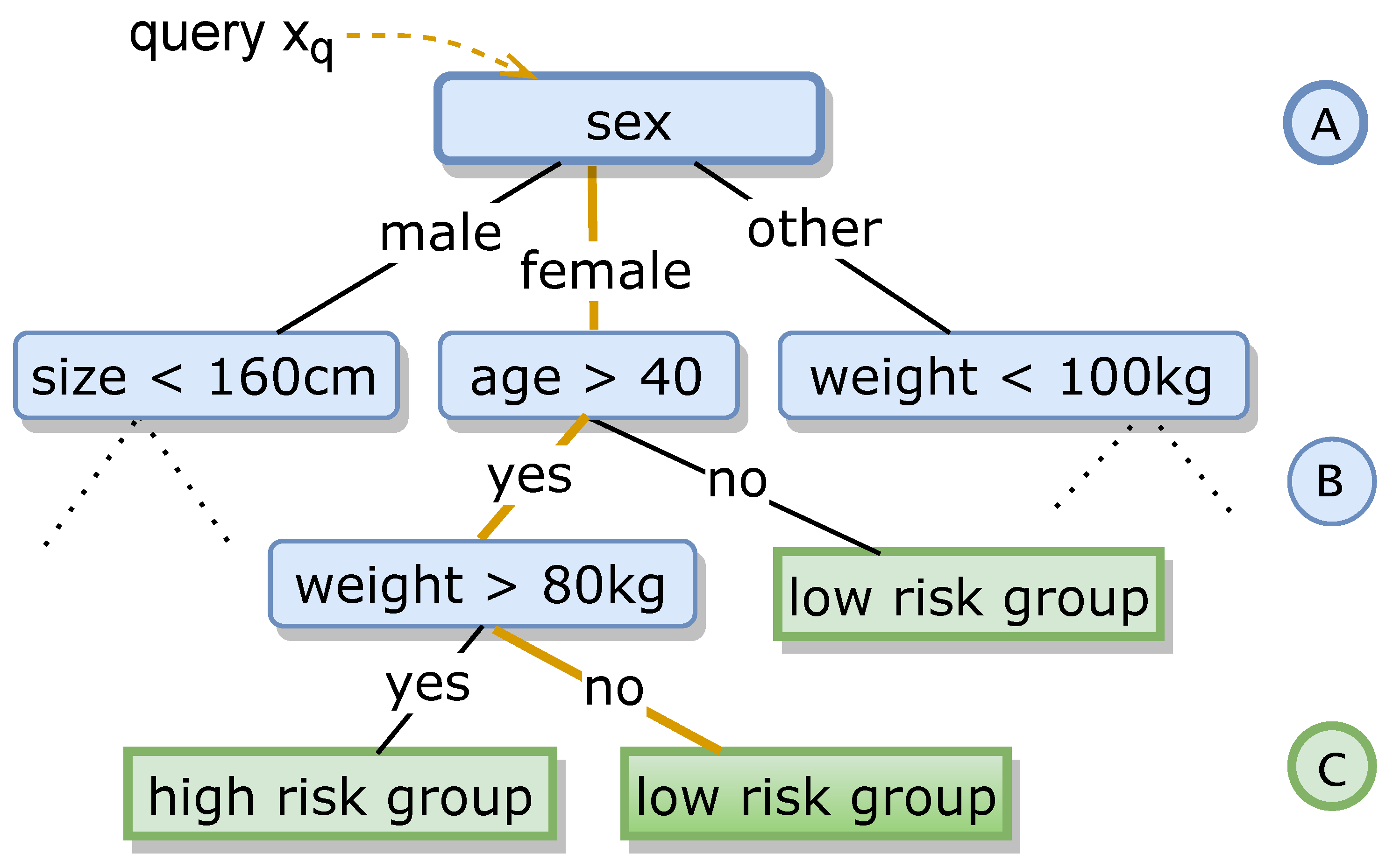
2.5. Decision Trees
2.6. Surrogate Models
2.7. Ensemble Learning and Dynamic Selection
3. The League of Experts Classifier
3.1. Basic Definitions and Model Formulation
3.1.1. Class of Assignment Functions
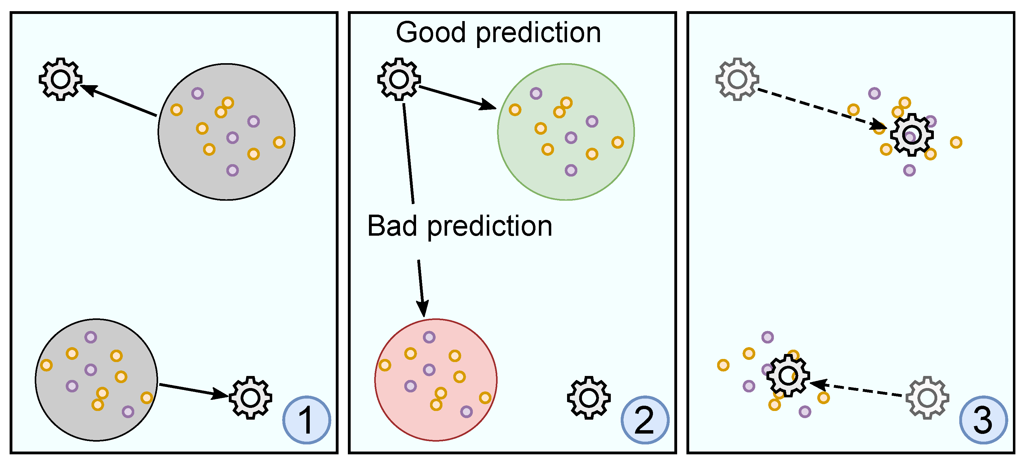
3.1.2. Algorithm Training
| Algorithm 1: Basic League of Experts Training Procedure |
 |
 |
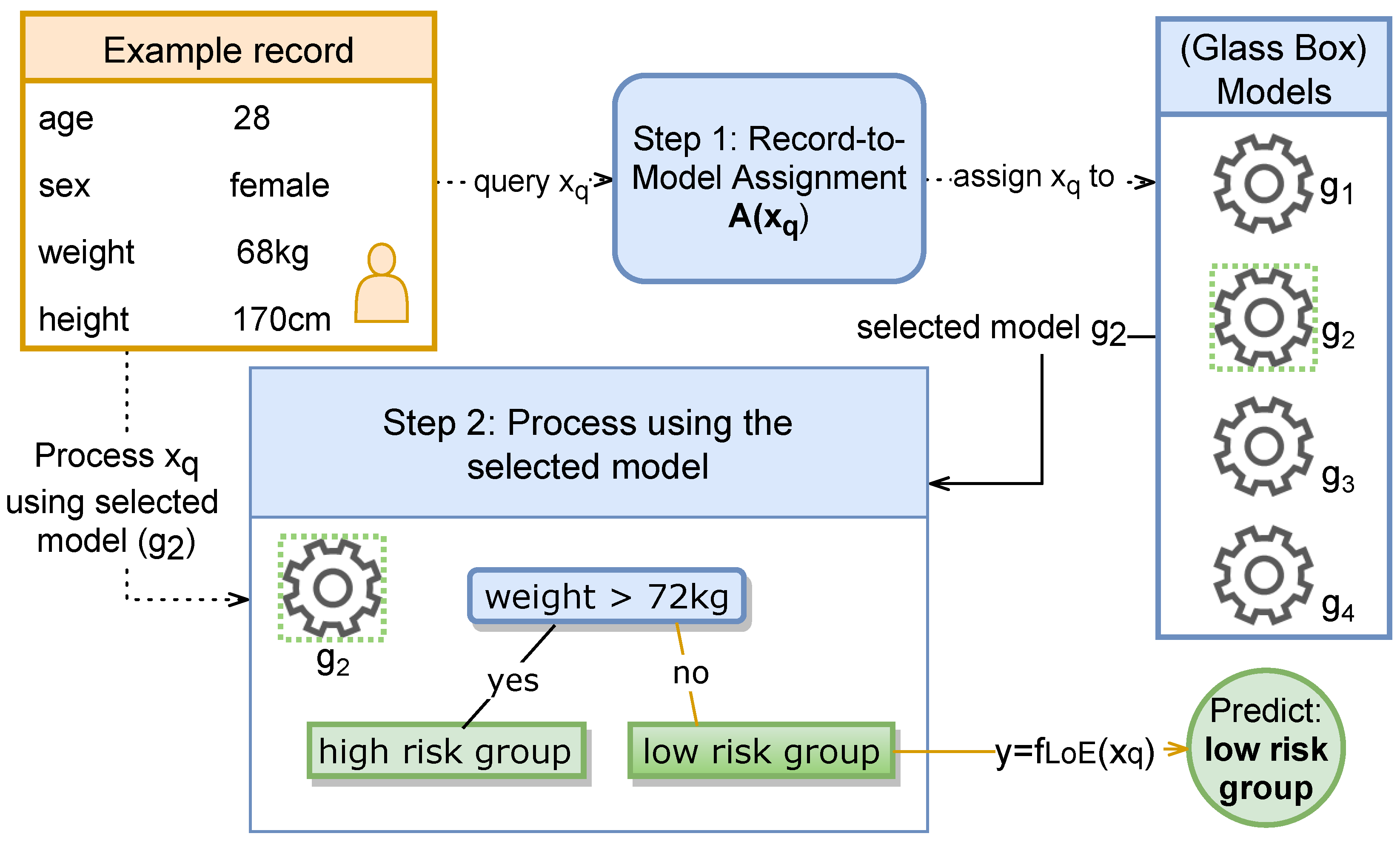
3.1.3. LoE Inference
3.2. Deriving Explanations
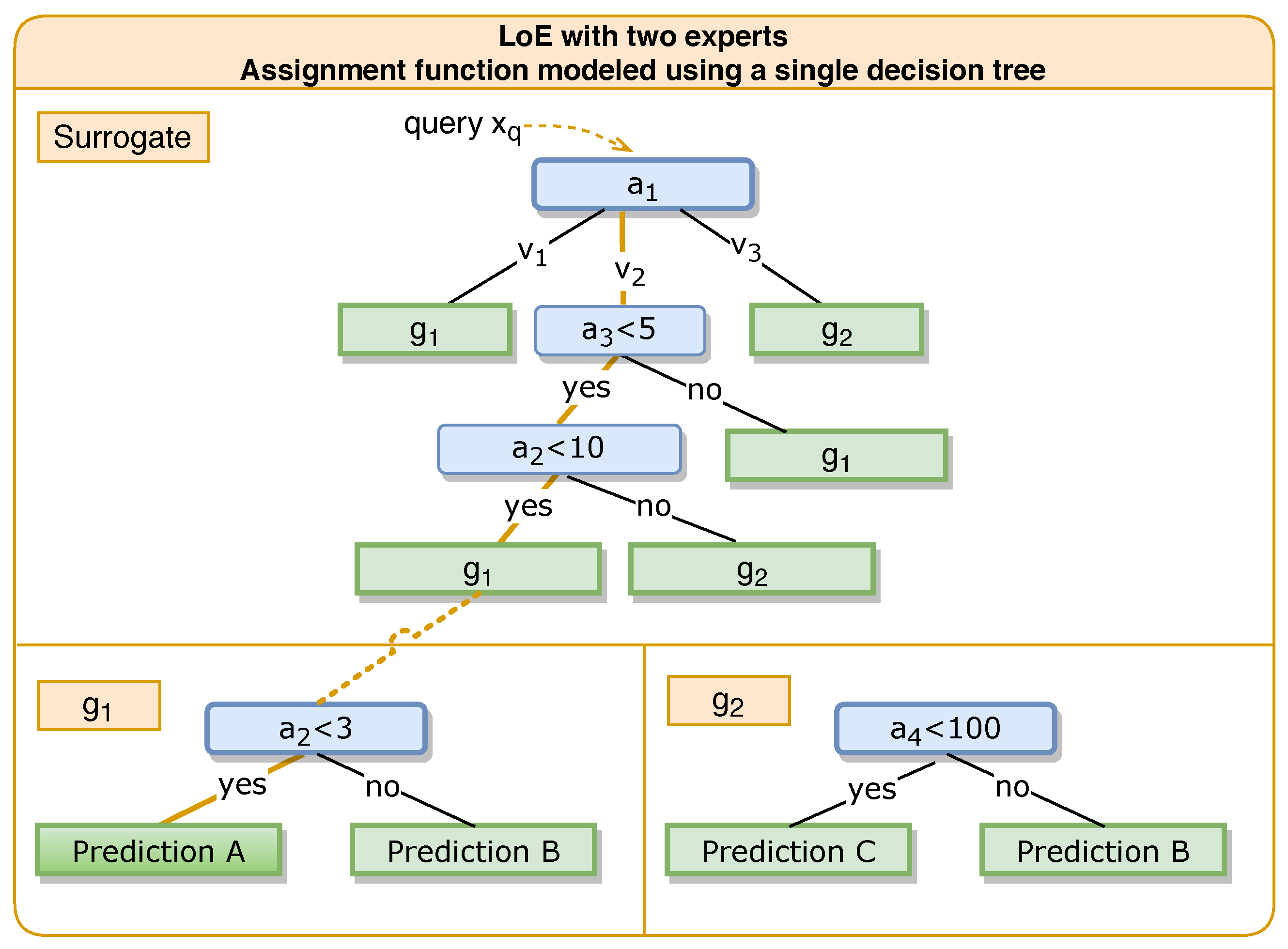
3.2.1. Making the Assignment Function Explainable
3.2.2. The Surrogate’s Faithfulness
3.2.3. Decision-Tree-Related Notation
3.2.4. Complexity of a Decision Tree
3.3. Reducing the Complexity of Explanations
3.3.1. Feature Space Reduction
3.3.2. Projections Obtained from Leveraging LoE’s Properties
3.3.3. Concrete Calculation of Feature Importances
3.4. Runtime Analysis
- T = number of iterations
- = ensemble of experts
- = labeled dataset
- = training complexity for model g for data
- = evaluation complexity for model g for data
3.5. LoE as a Rule Set Learner—RuleLoE
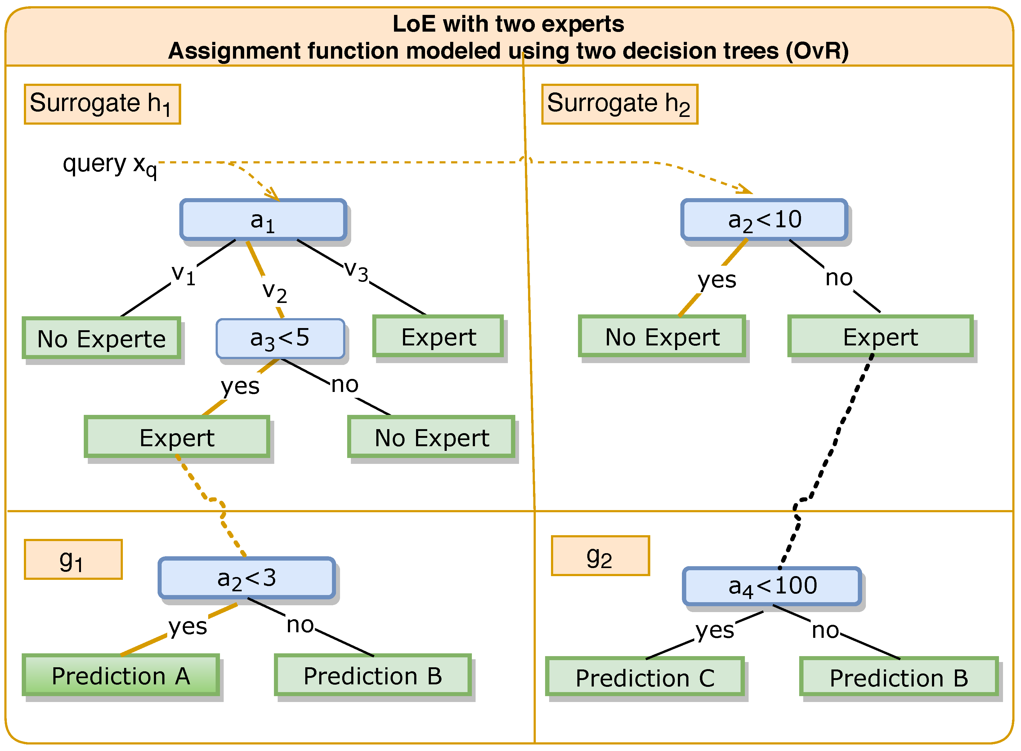
3.5.1. One-versus-Rest Surrogate
3.5.2. Query Strategy
- 1.
- Rank rules by descending precision (and coverage on tie).
- 2.
- Assign to the covering rule with the lowest rank.
- 3.
- If no rule covers , return the rule with the highest fraction of clauses being evaluated as “true” (partial rule coverage) with preference given to the rule with higher precision on ties.
4. Test Results, Evaluation, and Discussion
- Example dataset 1: UCI breast cancer
- Example dataset 2: HELOC
- Example dataset 3: KEEL
- Used Software
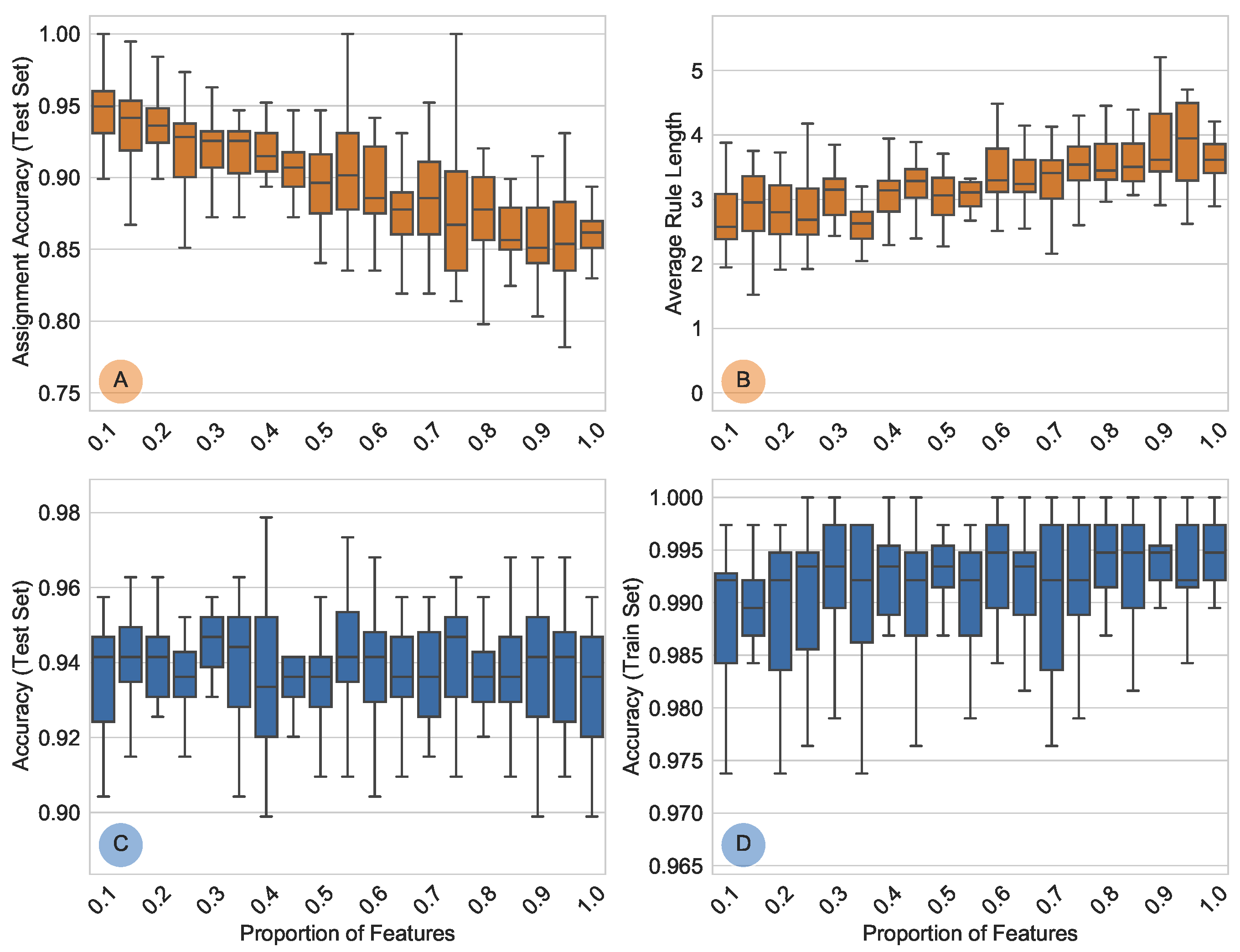
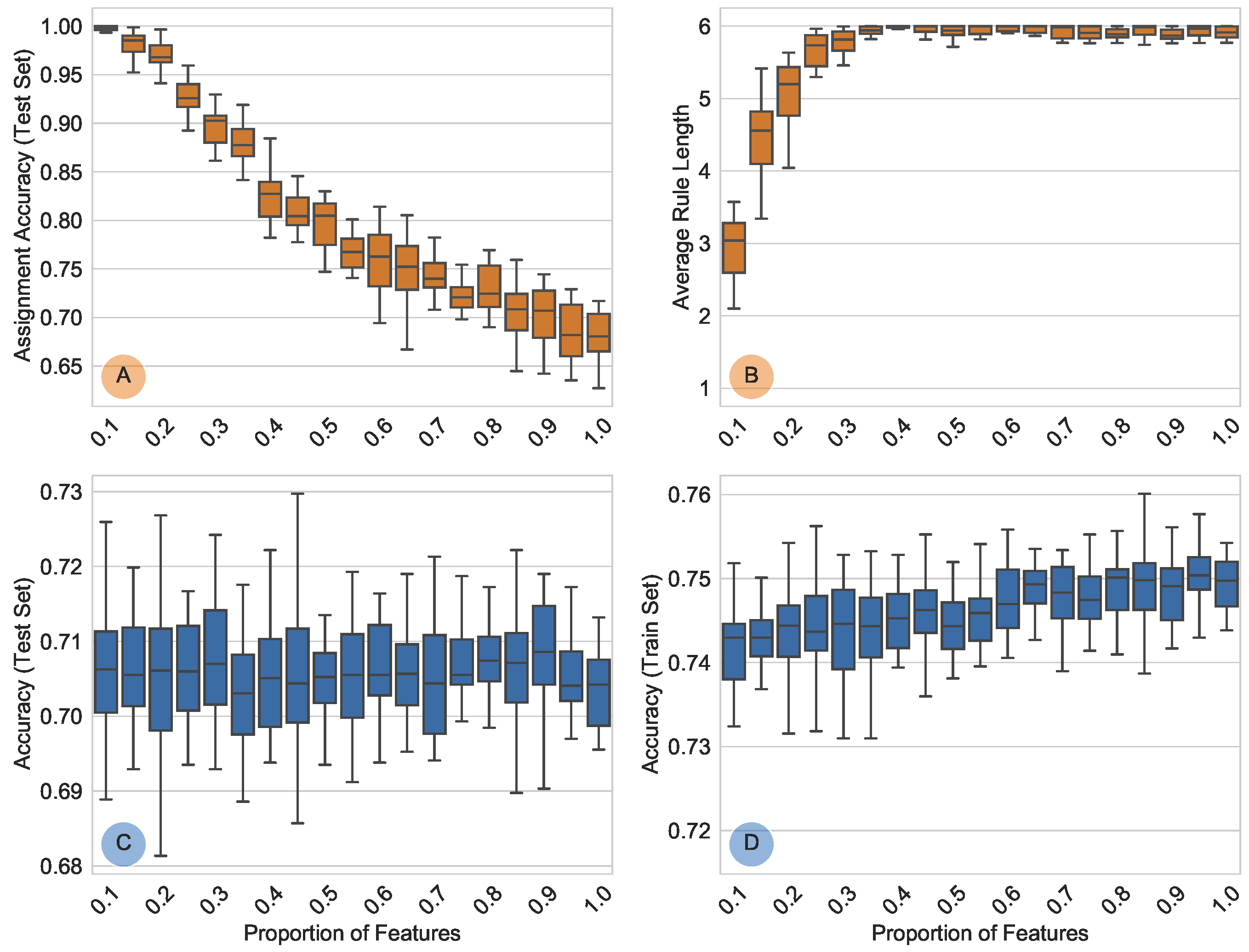
4.1. Feature Space Reduction
- Test Results
4.2. Rule Set Generation with RuleLoE
- Random forest: 100/∞
- Gradient boosting: 100/3
- Extra trees: 100/∞
- AdaBoost: 50/1
4.2.1. UCI Breast Cancer Dataset
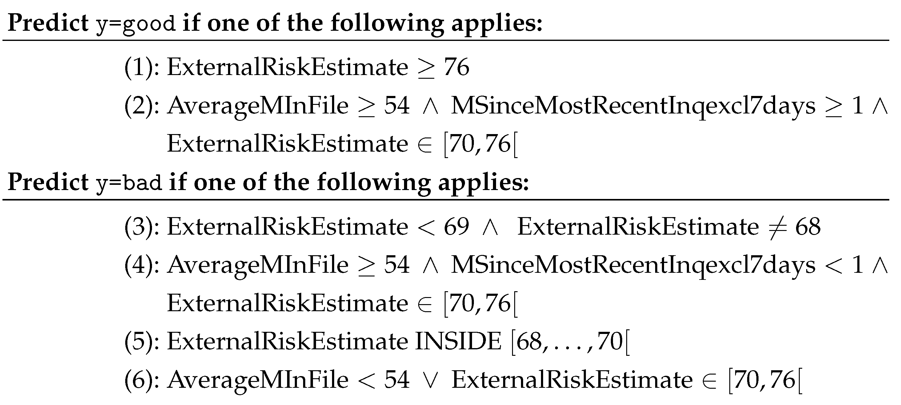
4.2.2. FICO Dataset
4.2.3. The KEEL Dataset
5. Conclusions and Outlook
Author Contributions
Funding
Institutional Review Board Statement
Informed Consent Statement
Data Availability Statement
Conflicts of Interest
Abbreviations
| ANN | artificial neural network |
| BRCG | Boolean decision rules via column generation |
| CART | classification and regression trees algorithm |
| DCS | dynamic classifier selection |
| DES | dynamic ensemble selection |
| DS | dynamic selection |
| DSEL | split of training data used in some MCS algorithms |
| ICE | individual conditional expectation plots |
| k-NN | k-nearest neighbors |
| LoE | League of Experts |
| MCS | multiple classifier system |
| ML | machine Learning |
| MLP | multilayer perceptron |
| OvR | one-versus-rest |
| PDP | partial dependence plots |
| RuleLoE | League of Experts rule set learner |
| SVC | support vector classifier |
| SVM | support vector machine |
| TreeSHAP | decision-tree-based SHAP |
| XAI | explainable artificial intelligence |
| XML | explainable machine learning |
References
- Maurer, M.; Gerdes, J.C.; Lenz, B.; Winner, H. Autonomous Driving; Springer: Berlin/Heidelberg, Germany, 2016. [Google Scholar]
- Haynes, R.B.; Wilczynski, N.L. Effects of computerized clinical decision support systems on practitioner performance and patient outcomes: Methods of a decision-maker-researcher partnership systematic review. Implement. Sci. IS 2010, 5, 12. [Google Scholar] [CrossRef] [PubMed]
- Bennett Moses, L.; Chan, J. Algorithmic prediction in policing: Assumptions, evaluation, and accountability. Polic. Soc. 2018, 28, 806–822. [Google Scholar] [CrossRef]
- Goodman, B.; Flaxman, S. European Union regulations on algorithmic decision-making and a “right to explanation”. AI Mag. 2017, 38, 50–57. [Google Scholar] [CrossRef]
- Deeks, A. The Judicial Demand for Explainable Artificial Intelligence. Columbia Law Rev. 2019, 119, 1829–1850. [Google Scholar]
- Doshi-Velez, F.; Kortz, M.; Budish, R.; Bavitz, C.; Gershman, S.; O’Brien, D.; Schieber, S.; Waldo, J.; Weinberger, D.; Wood, A. Accountability of AI Under the Law: The Role of Explanation. arXiv 2017, arXiv:1711.01134. [Google Scholar] [CrossRef]
- Rudin, C. Stop explaining black box machine learning models for high stakes decisions and use interpretable models instead. Nat. Mach. Intell. 2019, 1, 206–215. [Google Scholar] [CrossRef] [PubMed]
- Swartout, W.; Paris, C.; Moore, J. Explanations in knowledge systems: Design for explainable expert systems. IEEE Expert 1991, 6, 58–64. [Google Scholar] [CrossRef]
- Paris, C.L. Generation and explanation: Building an explanation facility for the explainable expert systems framework. In Natural Language Generation in Artificial Intelligence and Computational Linguistics; Springer: Berlin/Heidelberg, Germany, 1991; pp. 49–82. [Google Scholar]
- Confalonieri, R.; Coba, L.; Wagner, B.; Besold, T.R. A historical perspective of explainable Artificial Intelligence. Wiley Interdiscip. Rev. Data Min. Knowl. Discov. 2021, 11, e1391. [Google Scholar] [CrossRef]
- Longo, L.; Brcic, M.; Cabitza, F.; Choi, J.; Confalonieri, R.; Del Ser, J.; Guidotti, R.; Hayashi, Y.; Herrera, F.; Holzinger, A.; et al. Explainable artificial intelligence (XAI) 2.0: A manifesto of open challenges and interdisciplinary research directions. arXiv 2023, arXiv:2310.19775. [Google Scholar]
- Markus, A.F.; Kors, J.A.; Rijnbeek, P.R. The role of explainability in creating trustworthy artificial intelligence for health care: A comprehensive survey of the terminology, design choices, and evaluation strategies. J. Biomed. Inform. 2021, 113, 103655. [Google Scholar] [CrossRef]
- Zini, J.E.; Awad, M. On the explainability of natural language processing deep models. ACM Comput. Surv. 2022, 55, 1–31. [Google Scholar] [CrossRef]
- Band, S.S.; Yarahmadi, A.; Hsu, C.C.; Biyari, M.; Sookhak, M.; Ameri, R.; Dehzangi, I.; Chronopoulos, A.T.; Liang, H.W. Application of explainable artificial intelligence in medical health: A systematic review of interpretability methods. Inform. Med. Unlocked 2023, 40, 101286. [Google Scholar] [CrossRef]
- Ali, S.; Abuhmed, T.; El-Sappagh, S.; Muhammad, K.; Alonso-Moral, J.M.; Confalonieri, R.; Guidotti, R.; Del Ser, J.; Díaz-Rodríguez, N.; Herrera, F. Explainable Artificial Intelligence (XAI): What we know and what is left to attain Trustworthy Artificial Intelligence. Inf. Fusion 2023, 99, 101805. [Google Scholar] [CrossRef]
- Crook, B.; Schlüter, M.; Speith, T. Revisiting the performance-explainability trade-off in explainable artificial intelligence (XAI). In Proceedings of the 2023 IEEE 31st International Requirements Engineering Conference Workshops (REW), Hannover, Germany, 4–5 September 2023; IEEE: Piscataway, NJ, USA, 2023; pp. 316–324. [Google Scholar]
- Hastie, T.; Tibshirani, R.; Friedman, J.; Franklin, J. The elements of statistical learning: Data mining, inference and prediction. Math. Intell. 2005, 27, 83–85. [Google Scholar]
- Cruz, R.M.O.; Sabourin, R.; Cavalcanti, G.D.C. Dynamic classifier selection: Recent advances and perspectives. Inf. Fusion 2018, 41, 195–216. [Google Scholar] [CrossRef]
- Breiman, L. Bagging predictors. Mach. Learn. 1996, 24, 123–140. [Google Scholar] [CrossRef]
- Guidotti, R.; Monreale, A.; Ruggieri, S.; Turini, F.; Giannotti, F.; Pedreschi, D. A survey of methods for explaining black box models. ACM Comput. Surv. (CSUR) 2018, 51, 1–42. [Google Scholar] [CrossRef]
- Adadi, A.; Berrada, M. Peeking inside the black-box: A survey on explainable artificial intelligence (XAI). IEEE Access 2018, 6, 52138–52160. [Google Scholar] [CrossRef]
- Loyola-Gonzalez, O. Black-box vs. white-box: Understanding their advantages and weaknesses from a practical point of view. IEEE Access 2019, 7, 154096–154113. [Google Scholar] [CrossRef]
- Bodria, F.; Giannotti, F.; Guidotti, R.; Naretto, F.; Pedreschi, D.; Rinzivillo, S. Benchmarking and survey of explanation methods for black box models. Data Min. Knowl. Discov. 2023, 37, 1719–1778. [Google Scholar] [CrossRef]
- LeCun, Y.; Bengio, Y.; Hinton, G. Deep learning. Nature 2015, 521, 436. [Google Scholar] [CrossRef]
- Canziani, A.; Paszke, A.; Culurciello, E. An Analysis of Deep Neural Network Models for Practical Applications. arXiv 2016, arXiv:1605.07678. [Google Scholar]
- Drucker, H.; Burges, C.J.C.; Kaufman, L.; Smola, A.J.; Vapnik, V. Support vector regression machines. In Proceedings of the Advances in Neural Information Processing Systems, Denver, CO, USA, 2–5 December 1996; pp. 155–161. [Google Scholar]
- Freund, Y.; Schapire, R.E. A Decision-Theoretic Generalization of On-Line Learning and an Application to Boosting. J. Comput. Syst. Sci. 1997, 55, 119–139. [Google Scholar] [CrossRef]
- Breiman, L. Random Forests. Mach. Learn. 2001, 45, 5–32. [Google Scholar] [CrossRef]
- Breiman, L.; Friedman, J.H.; Olshen, R.A.; Stone, C.J. Classification And Regression Trees; Routledge: London, UK, 2017. [Google Scholar]
- Das, A.; Rad, P. Opportunities and challenges in explainable artificial intelligence (xai): A survey. arXiv 2020, arXiv:2006.11371. [Google Scholar]
- Hassija, V.; Chamola, V.; Mahapatra, A.; Singal, A.; Goel, D.; Huang, K.; Scardapane, S.; Spinelli, I.; Mahmud, M.; Hussain, A. Interpreting black-box models: A review on explainable artificial intelligence. Cogn. Comput. 2024, 16, 45–74. [Google Scholar] [CrossRef]
- Altman, N.S. An Introduction to Kernel and Nearest-Neighbor Nonparametric Regression. Am. Stat. 1992, 46, 175–185. [Google Scholar] [CrossRef]
- Friedman, N.; Geiger, D.; Goldszmidt, M. Bayesian Network Classifiers. Mach. Learn. 1997, 29, 131–163. [Google Scholar] [CrossRef]
- Lakkaraju, H.; Bach, S.H.; Leskovec, J. Interpretable Decision Sets: A Joint Framework for Description and Prediction. In Proceedings of the 22nd ACM SIGKDD International Conference on Knowledge Discovery and Data Mining, New York, NY, USA, 13–17 August 2016; KDD ’16. pp. 1675–1684. [Google Scholar]
- Clark, P.; Niblett, T. The CN2 Induction Algorithm. Mach. Learn. 1989, 3, 261–283. [Google Scholar] [CrossRef]
- Cohen, W.W. Fast Effective Rule Induction. In Proceedings of the Twelfth International Conference on Machine Learning, Tahoe City, CA, USA, 9–12 July 1995; Morgan Kaufmann: Burlington, MA, USA, 1995; pp. 115–123. [Google Scholar]
- Yang, H.; Rudin, C.; Seltzer, M. Scalable Bayesian Rule Lists. arXiv 2016, arXiv:1602.08610. [Google Scholar]
- Dash, S.; Gunluk, O.; Wei, D. Boolean Decision Rules via Column Generation. In Advances in Neural Information Processing Systems 31; Bengio, S., Wallach, H., Larochelle, H., Grauman, K., Cesa-Bianchi, N., Garnett, R., Eds.; Curran Associates, Inc.: New York, NY, USA, 2018; pp. 4655–4665. [Google Scholar]
- Ribeiro, M.T.; Singh, S.; Guestrin, C. Why Should I Trust You? Explaining the Predictions of Any Classifier. arXiv 2016, arXiv:1602.04938. [Google Scholar]
- Ribeiro, M.T.; Singh, S.; Guestrin, C. Anchors: High-Precision Model-Agnostic Explanations. In Proceedings of the Thirty-Second AAAI Conference on Artificial Intelligence, New Orleans, LA, USA, 2–7 February 2018. [Google Scholar]
- Lundberg, S.M.; Lee, S. A Unified Approach to Interpreting Model Predictions. In Proceedings of the 31st International Conference on Neural Information Processing Systems, Red Hook, NY, USA, 4–9 December 2017; NIPS’17. pp. 4768–4777. [Google Scholar]
- Molnar, C. Interpretable Machine Learning: A Guide for Making Black Box Models Interpretable; Lulu: Morisville, NC, USA, 2019. [Google Scholar]
- Lundberg, S.M.; Erion, G.G.; Lee, S. Consistent Individualized Feature Attribution for Tree Ensembles. arXiv 2018, arXiv:1802.03888. [Google Scholar]
- Buhrmester, V.; Münch, D.; Arens, M. Analysis of Explainers of Black Box Deep Neural Networks for Computer Vision: A Survey. arXiv 2019, arXiv:1911.12116. [Google Scholar] [CrossRef]
- Arrieta, A.B.; Díaz-Rodríguez, N.; Ser, J.D.; Bennetot, A.; Tabik, S.; Barbado, A.; García, S.; Gil-López, S.; Molina, D.; Benjamins, R.; et al. Explainable Artificial Intelligence (XAI): Concepts, Taxonomies, Opportunities and Challenges toward Responsible AI. Inf. Fusion 2019, 58, 82–115. [Google Scholar] [CrossRef]
- Fürnkranz, J.; Gamberger, D.; Lavrač, N. Foundations of Rule Learning; Springer Publishing Company, Incorporated: Berlin/Heidelberg, Germany, 2014. [Google Scholar]
- Gunning, D. DARPA’s Explainable Artificial Intelligence (XAI) Program. In Proceedings of the 24th International Conference on Intelligent User Interfaces, New York, NY, USA, 16–20 March 2019; IUI ’19. p. ii. [Google Scholar]
- Kotsiantis, S.B. Decision trees: A recent overview. Artif. Intell. Rev. 2013, 39, 261–283. [Google Scholar] [CrossRef]
- Freitas, A.A. Comprehensible classification models. ACM SIGKDD Explor. Newsl. 2014, 15, 1–10. [Google Scholar] [CrossRef]
- Alizadeh, R.; Allen, J.K.; Mistree, F. Managing computational complexity using surrogate models: A critical review. Res. Eng. Des. 2020, 31, 275–298. [Google Scholar] [CrossRef]
- Heider, K.G. The Rashomon effect: When ethnographers disagree. Am. Anthropol. 1988, 90, 73–81. [Google Scholar] [CrossRef]
- Dong, X.; Yu, Z.; Cao, W.; Shi, Y.; Ma, Q. A survey on ensemble learning. Front. Comput. Sci. 2020, 14, 241–258. [Google Scholar] [CrossRef]
- Mienye, I.D.; Sun, Y. A survey of ensemble learning: Concepts, algorithms, applications, and prospects. IEEE Access 2022, 10, 99129–99149. [Google Scholar] [CrossRef]
- Arya, V.; Bellamy, R.K.E.; Chen, P.-Y.; Dhurandhar, A.; Hind, M.; Hoffman, S.C.; Houde, S.; Liao, Q.V.; Luss, R.; Mojsilović, A.; et al. One Explanation Does Not Fit All: A Toolkit and Taxonomy of AI Explainability Techniques. arXiv 2019, arXiv:1909.03012. [Google Scholar]
- Alvarez-Melis, D.; Jaakkola, T.S. Towards Robust Interpretability with Self-Explaining Neural Networks. arXiv 2018, arXiv:1806.07538. [Google Scholar]
- Geurts, P.; Ernst, D.; Wehenkel, L. Extremely randomized trees. Mach. Learn. 2006, 63, 3–42. [Google Scholar] [CrossRef]
- Safavian, S.R.; Landgrebe, D. A survey of decision tree classifier methodology. IEEE Trans. Syst. Man Cybern. 1991, 21, 660–674. [Google Scholar] [CrossRef]
- Street, W.N.; Wolberg, W.H.; Mangasarian, O.L. Nuclear feature extraction for breast tumor diagnosis. In Proceedings of the Biomedical Image Processing and Biomedical Visualization, San Jose, CA, USA, 1–4 February 1993; Volume 1905, pp. 861–870. [Google Scholar]
- Wei, D.; Dash, S.; Gao, T.; Gunluk, O. Generalized Linear Rule Models. In Proceedings of the 36th International Conference on Machine Learning, Long Beach, CA, USA, 9–15 June 2019; Chaudhuri, K., Salakhutdinov, R., Eds.; Proceedings of Machine Learning Research. Volume 97, pp. 6687–6696. [Google Scholar]
- Chen, C.; Lin, K.; Rudin, C.; Shaposhnik, Y.; Wang, S.; Wang, T. An Interpretable Model with Globally Consistent Explanations for Credit Risk. arXiv 2018, arXiv:1811.12615. [Google Scholar]
- Derrac, J.; Garcia, S.; Sanchez, L.; Herrera, F. Keel data-mining software tool: Data set repository, integration of algorithms and experimental analysis framework. J. Mult.Valued Log. Soft Comput. 2015, 17, 255–287. [Google Scholar]


| Dataset | Data Points | Features | Classes | Class Entropy |
|---|---|---|---|---|
| banana | 5300 | |||
| coil2000 | 9822 | 85 | ||
| marketing | 6876 | 13 | ||
| mushroom | 5644 | 98 | ||
| optdigits | 5620 | 64 | 10 | |
| page-blocks | 5472 | 10 | ||
| phoneme | 5404 | |||
| ring | 7400 | 20 | ||
| satimage | 6435 | 36 | ||
| texture | 5500 | 40 | 11 | |
| thyroid | 7200 | 21 | ||
| twonorm | 7400 | 20 |
| Algorithm | # Rules | ⌀ Rules | Rule Coverage (%) | Accuracy (%) | |
|---|---|---|---|---|---|
| RuleLoE | 10 | / | / | ||
| RIPPER | malignant | 9 | / | / | |
| RIPPER | benign | 13 | / | / | |
| BRCG | malignant | 5 | / | / | |
| BRCG | benign | 5 | / | / | |
| CART | 7 | / | / | ||
| Random forest | default | - | - | - | / |
| Random forest | adjusted | - | - | - | / |
| Gradient boosting | default | - | - | - | / |
| Gradient boosting | adjusted | - | - | - | / |
| Extra trees | default | - | - | - | / |
| Extra trees | adjusted | - | - | - | / |
| AdaBoost | default | - | - | - | / |
| AdaBoost | adjusted | - | - | - | / |
| SVC | - | - | - | / | |
| MLP | - | - | - | / |
| Algorithm | # Rules | ⌀ Rules | Rule Coverage (%) | Accuracy (%) | |
|---|---|---|---|---|---|
| RuleLoE | 6 | / | / | ||
| RIPPER | bad | 18 | / | / | |
| RIPPER | good | 25 | / | / | |
| BRCG | bad | 1 | / | / | |
| BRCG | good | 2 | / | / | |
| CART | 21 | / | / | ||
| Random forest | default | - | - | - | / |
| Random forest | adjusted | - | - | - | / |
| Gradient boosting | default | - | - | - | / |
| Gradient boosting | adjusted | - | - | - | / |
| Extra trees | default | - | - | - | / |
| Extra trees | adjusted | - | - | - | / |
| AdaBoost | default | - | - | - | |
| AdaBoost | adjusted | - | - | - | |
| SVC | - | - | - | / | |
| MLP | - | - | - | / |
| Dataset | Random Forest (%) | LoE (%) | RuleLoE (%) | Assignment Accuracy (%) | # Rules (⌀ Length) |
|---|---|---|---|---|---|
| banana | / | / | / | / | 10 ( |
| coil2000 | / | / | / | / | ( |
| marketing | / | / | / | / | ( |
| mushroom | / | / | / | / | ( |
| optdigits | / | / | / | / | ( |
| page-blocks | / | / | / | / | ( |
| phoneme | / | / | / | / | ( |
| ring | / | / | / | / | ( |
| satimage | / | / | / | / | 10 ( |
| texture | / | / | / | / | ( |
| thyroid | / | / | / | / | ( |
| twonorm | / | / | / | / | ( |
| Average | / | / | / | / | () |
Disclaimer/Publisher’s Note: The statements, opinions and data contained in all publications are solely those of the individual author(s) and contributor(s) and not of MDPI and/or the editor(s). MDPI and/or the editor(s) disclaim responsibility for any injury to people or property resulting from any ideas, methods, instructions or products referred to in the content. |
© 2024 by the authors. Licensee MDPI, Basel, Switzerland. This article is an open access article distributed under the terms and conditions of the Creative Commons Attribution (CC BY) license (https://creativecommons.org/licenses/by/4.0/).
Share and Cite
Vogel, R.; Schlosser, T.; Manthey, R.; Ritter, M.; Vodel, M.; Eibl, M.; Schneider, K.A. A Meta Algorithm for Interpretable Ensemble Learning: The League of Experts. Mach. Learn. Knowl. Extr. 2024, 6, 800-826. https://doi.org/10.3390/make6020038
Vogel R, Schlosser T, Manthey R, Ritter M, Vodel M, Eibl M, Schneider KA. A Meta Algorithm for Interpretable Ensemble Learning: The League of Experts. Machine Learning and Knowledge Extraction. 2024; 6(2):800-826. https://doi.org/10.3390/make6020038
Chicago/Turabian StyleVogel, Richard, Tobias Schlosser, Robert Manthey, Marc Ritter, Matthias Vodel, Maximilian Eibl, and Kristan Alexander Schneider. 2024. "A Meta Algorithm for Interpretable Ensemble Learning: The League of Experts" Machine Learning and Knowledge Extraction 6, no. 2: 800-826. https://doi.org/10.3390/make6020038
APA StyleVogel, R., Schlosser, T., Manthey, R., Ritter, M., Vodel, M., Eibl, M., & Schneider, K. A. (2024). A Meta Algorithm for Interpretable Ensemble Learning: The League of Experts. Machine Learning and Knowledge Extraction, 6(2), 800-826. https://doi.org/10.3390/make6020038