Abstract
Squash is a sport where referee decisions are essential to the game. However, these decisions are very subjective in nature. Disputes, both from the players and the audience, regularly occur because the referee made a controversial call. In this study, we propose automating the referee decision process through machine learning. We trained neural networks to predict such decisions using data from 400 referee decisions acquired through extensive video footage reviewing and labeling. Six positional values were extracted, including the attacking player’s position, the retreating player’s position, the ball’s position in the frame, the ball’s projected first bounce, the ball’s projected second bounce, and the attacking player’s racket head position. We calculated nine additional distance values, such as the distance between players and the distance from the attacking player’s racket head to the ball’s path. Models were trained on Wolfram Mathematica and Python using these values. The best Wolfram Mathematica model and the best Python model achieved accuracies of 86% ± 3.03% and 85.2% ± 5.1%, respectively. These accuracies surpass 85%, demonstrating near-human performance. Our model has great potential for improvement as it is currently trained with limited, unbalanced data (400 decisions) and lacks crucial data points such as time and speed. The performance of our model is almost surely going to improve significantly with a larger training dataset. Unlike human referees, machine learning models follow a consistent standard, have unlimited attention spans, and make decisions instantly. If the accuracy is improved in the future, the model can potentially serve as an extra refereeing official for both professional and amateur squash matches. Both the analysis of referee decisions in squash and the proposal to automate the process using machine learning is unique to this study.
1. Introduction
1.1. What Is Squash?
Squash is a racket sport played by two people on a four-wall court. The players alternate striking the ball, and the goal is to keep the ball in bounds while making it impossible for the opponent to retrieve it before two bounces on the floor. Every shot should hit the front wall before it bounces on the ground for the shot to be deemed an in-bound shot, while the sidewalls could be used to change the ball’s trajectory before or after the ball has reached the front wall. Squash is considered one of the most physically demanding sports, as the rallies are frequent and last for long periods of time.
1.2. Interferences and Referee Decisions
Because the two players are playing the game on one court, an inevitable aspect of squash is interference. The presence of one player, through inaccurate positioning or movement, can affect or prevent the shot of another player—for example, when player A strikes the ball, but the ball lands back next to player A, and player A is not able to get out of the way (in squash terms, “clear the ball”). In this case, player B would have hit player A if player B attempted to hit the ball. This is a common example of interference. When players are stopped due to interference, the player who is supposed to strike the ball can choose to appeal to the referee for a decision.
In these situations, referees decide to fairly punish or reward players for the interference that has occurred. In squash, there are three possible decisions: Stroke, Yes Let, and No Let. A Stroke for the appealing player awards a point to the player, a Yes Let means it is necessary to replay the point, and a No Let for the appealing player awards a point to the other player.
The Professional Squash Association (PSA) defines these decisions and their situations of applications as follows:
“Yes Let decision results in the rally being played again—with the referee deeming that the interference was accidental and both players have made an equal effort to allow play to continue.No Let decision is where the referee rules against the striker’s appeal and awards a point to the retreating player. In this situation, the referee deemed that the retreating player provided unobstructed access and that interference was minimal, therefore the appealing striker could have played a shot.Stroke is when the point is awarded to the appealing player. A stroke is awarded when the referee deems the incoming striker is in a position to play a shot, but suffers interference due to the outgoing player not making every effort to clear”.[1]
The ultimate guidelines for clearing a shot are explained by the PSA as follows:
“After playing a shot, players must make every effort to ‘clear the ball’ so that when the ball rebounds from the front wall, the opponent has both
- (A)
- (B)
- (C)
Therefore, in the above-mentioned situation of players A and B, player B would stop and appeal. The correct decision from the referee would be a Stroke to player B because player A had obstructed player B’s access to the ball. Therefore, player B would gain a point, and the match would continue with the next rally.
1.3. Controversies and Disputes
1.3.1. Regarding the Central Referee
Although all referees should strive for logical, unbiased decisions, the pace of squash and the complexity of professional players’ movements can make some decisions extremely difficult. An individual referee’s personal understanding of the game and the referee’s experience in the position can also affect the result. Although the PSA has introduced a video review system, many controversies still exist, both between players and referees and among the viewing audiences.
1.3.2. The Video Review System
The video review system consists of a real-time replay system and one video referee. Whenever a player wants to challenge a referee’s decision and, at the same time, has a “review remaining”, the tech crew replays the recording from the previous rally from multiple angles, and the video referee makes a decision based on the replay. The new decision can overrule or uphold the previous decision made by the central referee. The replay system allows the video referee to review the interference in slow motion and at various angles, and most of the time the review system can correct the calls. However, the video review can take a long time, including the time needed to retrieve the recordings and the time the video referee needs to fully understand the situation. This significantly disrupts the flow of the game. Therefore, the PSA only allows players one review per game, and if the player successfully reviews a decision, they will get another review. The disruption of the game is still a minor issue. After all, the decision is made by an isolated individual, and the biases and differences in understanding of the game could also affect the video referee in making these decisions. There are numerous cases in which a controversial call is upheld or an even more controversial decision is made after video review.
1.3.3. Controversies and Arguments
The PSA is struggling with refereeing problems as the sport grows bigger and more popular, and the issue remains relatively minor due to the video review system on the professional tour. However, junior and college squash are susceptible to controversial decisions as the referee’s words are the final judgment, and there is no way to reverse this decision. After all, decisions that go against the players’ and the viewers’ common sense undermine both the competition and the overall experience. The PSA has strived to solve this issue by updating referee guidelines and refining the video review system. However, these measures have not been very effective. There still regularly exists dissatisfaction from audiences as well as arguments between players and referees—see Figure 1, Figure 2 and Figure 3.
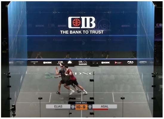
Figure 1.
Example of player interference [2].
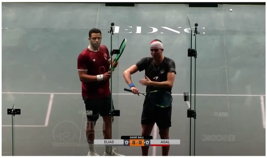
Figure 2.
Player unsatisfied with the decision, having opened the back door to argue with the referee (which would result in conduct warning if the referee does not want the discussion) [2].
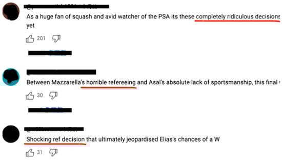
Figure 3.
Audience’s comments under a video on the Professional Squash Association’s YouTube channel commenting on their dissatisfaction with the refereeing work [2].
1.4. Machine Learning and Literature Review
One root cause of the controversy is the lack of exact measurement in referee decisions. Usually, referees make their decisions based on several evaluations: is there a clear path to the ball? Was the retrieving player blocked from the path to the ball? Could the player have hit the ball had there been no interference? Did the player show enough effort to play through the interference? Did the retreating player block access to the entire front wall? Was it due to safety that the player stopped to appeal?
Several crucial ideas exist: clear path, ability to retrieve, effort, blockage, and safety. All referees have different understandings of these concepts, which can result in different decisions. One referee might deem that a player is able to return the ball had there been no interference, but another referee might think the opposite. This disagreement in measures and the fundamental subjectivity underlying these decisions cause the never-ending disputes surrounding squash refereeing.
Machine learning, on the other hand, could eliminate these differences caused by referees’ subjectivity, since once the network is trained to have set parameters, the same situation would only result in the same decision. Though it has not specifically been applied to squash refereeing, machine learning has been widely used in sports applications.
For squash specifically, models have been trained to perform player detection and motion analysis [3]. Brumann’s research team investigated more than 250 human pose estimation convolutional neural networks (CNN) and found the five most effective models in the context of motion analysis for squash. The data being used were collected from publicly available squash videos, and Brumann’s team developed their own annotation tool and manually labeled frames and events. Using the labeled data and the trained CNNs, they were able to present heatmaps which depicted the court floor using a color scale and highlight areas according to the relative time for which a player occupied that location during play. Numerous general machine learning models used for motion detection have also been proposed. In 2013, a motion detection model was proposed utilizing machine learning and data clustering and achieved scene adaptive motion detection [4]. In 2016, a model capable of accurately detecting black and white soccer balls was produced using a series of heuristic region-of-interest identification techniques and supervised machine learning methods [5]. In 2021, a model based on YOLOv3 object detection was introduced and addressed the detection of small, fast-moving balls in sport video data [6].
Machine learning has also been applied to the sport of tennis to predict match outcomes [7]. Bayram trained and tested models using advanced machine learning paradigms such as multi-output regression and learning using privileged information on more than 83,000 men’s singles tennis matches between the years 1991 and 2020. The results outperform the existing methods in the literature and the current state-of-the-art models in tennis. In 2018, a tree-based boosting model was proposed to predict biathlon shooting performance [8]. In 2019, a model using the Random Forest algorithm obtained a precision of 0.857 and a recall of 0.750 in soccer match prediction [9]. The model was trained with data acquirable both after and during the match. In 2021, a deep-learning model featuring regression and classification analysis was trained to predict professional basketball players’ future performance and All-Star game selection [10].
In addition to detecting player motion and predicting match results, machine learning has also been utilized to predict shot success in table tennis [11]. In this study, Draschkowitz extracted features like the length and direction of strokes from the videos and trained classifiers to predict shot success and failure. After training, these classifiers are capable of predicting the success of strokes for a particular game and player and thus allow players and coaches to adapt to strategies more suitable to specific players.
On the other hand, previous studies have also commented on the inconsistency of referee decisions in competitive sports. In a seminal work on the influence of crowd noise on refereeing in soccer [12], researchers investigated the effect of home crowds on referees. They found a significant imbalance in decisions in favor of the home team when crowd noise is present. Although the difference between home and away players in squash is less noticeable compared to soccer, the crowd often favors one player over another, which may produce similar effects on a refereeing official. Furthermore, studies have surveyed the empirical literature on the behavior of referees in professional football and other sports and have found that referees often favor the home team in football, basketball, and baseball [13]. On the other hand, a study in 2018 investigated basketball referees’ decisions on potential offensive foul situations and found no evidence of favoritism granted to the home team, to star players, to high-reputation teams, or to physically small players being tackled by significantly larger opponents [14].
To acquire data for this study, we utilized a similar approach to the study “Using a Situation Awareness Approach to Determine Decision-Making Behavior in Squash” [15]. The researchers investigated the strategic nature of many shots in squash. They reviewed 41 recorded professional matches and analyzed every shot, excluding serves, returns of serves, and rally ending shots. They calculated four values from the video: time between player A’s shot and player B returning the shot (time); the distance player B moved to return player A’s shot (distance for B); the maximum velocity of player B from the moment player A hit the shot to player B returning the shot (max speed for B); and the distance player B was from the T at the moment player A hit the shot (B distance from T).
Through cluster analysis of the four values, six shot types (attempted winners, attack, pressure, pressing, maintain stability, and defense) were developed and differentiated through magnitudes of the four values. For example, if the distance from T exceeded 2.6 m, the time exceeded 1.7 s, the distance exceeded 4.0 m, and the speed exceeded 3.6 m/s, the shot was classified as the most threatening “attempted winner”. Using these metrics, the researchers were able to categorize the strategical usage of every shot that has been played in the 41 matches.
Through analyzing video footage and collecting numerical data, Murray’s research team was able to find meaningful results regarding the strategic purpose of different types of shots [15]. We propose using similar methods of data collection, in other words, analyzing video footage and collecting numerical data.
1.5. Objectives of This Study
The objective of this study is to investigate whether machine learning can be applied to predict (or make) squash referee decisions. As the current measures in place (decisions by humans) are causing controversies, we wish to explore the possibility of decisions by machine learning and, if possible, develop a model that can be utilized to perform real-life decision making in a squash match.
We intend this study to represent a forerunner of a fully automated decision system. The next stage of the project, left for the follow-up paper, is to implement real-time motion capture and decision analysis, ultimately leading to a functional system that runs in real-time without the need of human supervision.
2. Materials
2.1. Data Collection
2.1.1. The Professional Squash Association (PSA) YouTube Channel
As we aimed in this study to train a model to perform real-world decision making, the data needed to be collected from real-world decisions as well. As there are no suitable public datasets available, we collected data and constructed a dataset from scratch.
The PSA YouTube Channel uploads publicly available squash matches played by the best professional players in the world, and we reviewed these videos to collect our data [16]. Each individual decision was given by a professional PSA referee at a prestigious PSA Tournament broadcast on YouTube. Over the course of this study, more than twenty hours of footage were reviewed, and 400 decisions were collected from these publicly available matches. Each decision, depending on the complication of the situation, can take three to five minutes to label. We spent more than 25 h labeling the interferences for this study.
2.1.2. The Definition of “Moment” and Six Data Components
In reality, interference happens dynamically. In some interferences, players collide and stop moving, and in some, players try to move through after contact. As using video as the input in machine learning is extremely challenging computationally, in this paper, we collected positional data from the video after limiting it to a single frame, or a “moment”, which was defined to be the frame when the players first collide or when the ball enters the attacking player’s reach.
After a moment was selected, six data components were collected from the frame: the attacking player’s position, the retreating player’s position, the ball’s position in the frame, the ball’s projected first bounce, the ball’s projected second bounce, and the attacking player’s racket head position.
To collect these data, we used the tool DigitizeIt (https://www.digitizeit.xyz/ accessed on 8 September 2023)—see Figure 4. Inside DigitizeIt, a top-down view of a standard squash court was uploaded. The x-axis and the y-axis were defined to begin at the bottom left of the squash court. A standard squash court’s dimensions are 6.40 m in width and 9.75 m in length. The x-axis ranges from 0 (meters) to 6.40 (meters), and the y-axis ranges from 0 (meters) to 9.75 (meters).
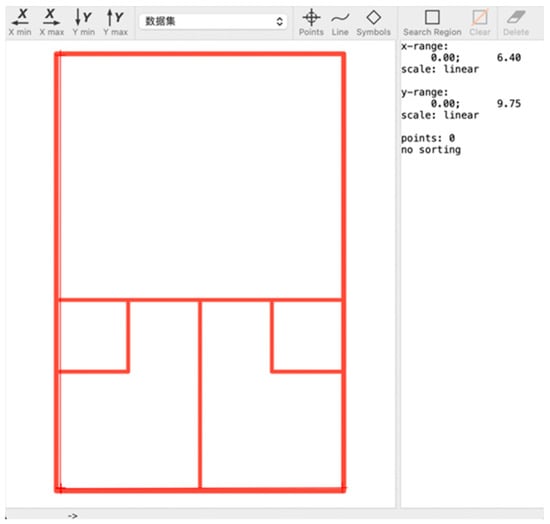
Figure 4.
Screenshot of the tool DigitizeIt.
To collect the six data components, we plotted a point on the graph of the squash court and DigitizeIt labelled its X and Y values. These values were then collected into our dataset together with the final decision. An example can be seen in Figure 5.
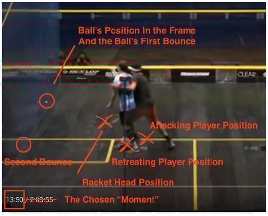
Figure 5.
(a) Data #3, Gaultier/Elshorbagy (players’ last names) 2014 ElGouna (tournament name) 13:50 YesLet [17]. The above format means the following: the data labeled “3” in our dataset. Taken from the match between Gregory Gaultier and Mohamed Elshorbagy in the 2014 ElGouna Championships. The interference happened at 13:50 in the video. The final decision was Yes Let. (b) Labeling for Data #3 in the tool DigitizeIt.
2.2. Data Distribution
Four hundred decisions were collected for this study, from multiple years and relating to multiple world-class players—see Figure 5, Figure 6 and Figure 7.
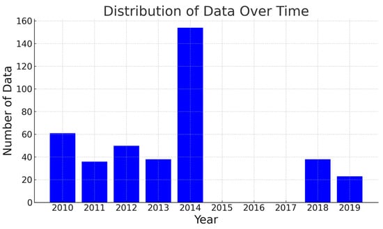
Figure 6.
Distribution of data over time.
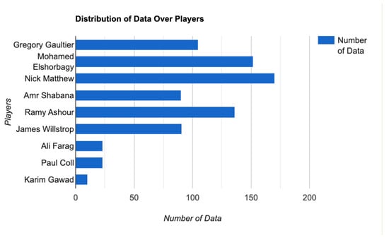
Figure 7.
Distribution of data over players.
The refereeing standard has shifted over the last decade. By awarding more Strokes and punishing more No Lets, the PSA intends to encourage fewer stoppages due to minimal interferences and more continuous plays. Such an effect is visible when reviewing matches from 2018 and 2019. Most of the data in this study were taken from 2010 to 2014, approximately when the video review system was available and when the refereeing standard was approximately consistent [18].
Due to factors such as the style of play, body strength, shot selection, dominance in the center of the court, and movement style, some players might be involved in more interferences than others. We tried to collect approximately similar numbers of decisions for each player involved.
The involved players are all among the best in the world. All have reached the world number one ranking at some point and are winners of major squash titles.
Due to the nature of the game, in any given match, there are more decisions ending in Yes Let than decisions ending in Stroke and No Let. Due to time constraints, we collected as many decisions as we could instead of discarding Yes Lets in search of No Lets and Strokes. As a result, our dataset consisted of 59 No Lets, 243 Yes Lets, and 98 Strokes—see Figure 8. It is clear that the dataset we used for this study is imbalanced. However, with future resources and efforts, this issue should be naturally resolved when the dataset is increased to a volume of 4000 or, perhaps, even 40,000 decisions.
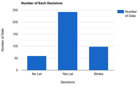
Figure 8.
Number of each decision.
3. Methods
3.1. Python, TensorFlow, and Wolfram Mathematica
In this study, we used two programming platforms to train the model: Python and Wolfram Language/Mathematica. The rationale for selecting Python was that it grants the ability to make many modifications to our model, including the network layers, nodes, different methods and functions, etc. The TensorFlow package constructs model layers with ease and provides freedom in modifying and fine-tuning the model. The combination of Python and TensorFlow has been widely used to train machine learning models. A study in 2019 used TensorFlow and achieved competitive performance results in classifying breast cancer malignancy [19]. A study in 2021 used TensorFlow and compared artificial neural networks and convolutional neural networks in image classification tasks [20].
Wolfram Mathematica, on the other hand, is easy to program and provides useful visualizations for model performances. Previous investigations have successfully used this platform to train powerful models. A study in 2022 used Wolfram Mathematica to develop an algorithm for localizing car license plates [21]. Another study in 2021 used its machine learning tools to produce COVID-19 projections from cumulative data for confirmed infected patients, vaccinated patients, and deaths in Mexico during 2021 [22].
The results of this study are, therefore, separated into the Python sections and the Wolfram Mathematica sections.
3.2. Neural Network
This study implemented machine learning through neural networks. Neural networks are machine learning algorithms inspired by the human brain and simulate the connection between neuron cells. Through layers of fully connected nodes, with each node performing a simple calculation task related to the multiplication and addition of parameters, the inputs undergo numerous transformations and reach a final value or the intended answer—see Figure 9. After being trained on a large dataset, a neural network can perform classification or clustering tasks in a relatively short period of time.
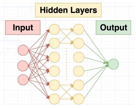
Figure 9.
Illustration of a neural network’s structure.
In order to resolve the issue of dataset imbalance, for every iteration of training/testing, the dataset was shuffled before being fed into the neural network model. Shuffling allowed the models to learn from all collected data points, and presented to us differences in model performance when a different percentage of each decision was used for training.
For this study, two different types of neural networks were utilized. For the Python models, a neural network consisting of 3 layers (64 × 128 × 3) of fully connected nodes was trained. The activation function for the first two layers was ReLU, and for the third layer, it was SoftMax. We chose the Adam optimizer and calculated the loss using sparse categorical cross-entropy. The epoch was set to be 15 for each training session. For the Wolfram Mathematica models, the built-in neural network training function was used. It was unclear what the numbers of the specific nodes and layers of the model were. The neural network utilized a gradient descent function to minimize the loss function, while further details were hidden in the machine learning black box.
3.3. Normalization
To pre-process the dataset, this study explored normalization. Normalization is a technique often used in machine learning to set a common scale for data with different ranges and measures. For this study specifically, although all X-values shared a common measure (0 m to 6.4 m) and all Y-values shared a common measure (0 m to 9.75 m), it was worth exploring whether the two axes could be normalized to allow the model to perform better.
3.4. Selection from the Six Data Components
As there exist many complicated reasons as to why a situation results in a decision, a neural network may be unable to learn all the relations between all data component values. Dropping out some less meaningful data components may, in fact, help the model to perform better, as too much information could act as noise to the model and impede its improvement. The method of data-dropping is a heuristic approach. It will be possible to delve deeper into the rationale behind the results with a much larger dataset.
3.5. Modified Data Points
We hypothesized that the initial six data components (or, the primitive data components) would not suffice to achieve the accuracy needed in real-life squash refereeing. There are more than six factors that decide what should be the right decision regarding an interference. Therefore, we decided to calculate a second layer of data using the primitive components acquired. The second layer of data components may be able to provide more insights into why and how a situation is considered one of the three decisions. More specifically, we used the primitive data components and calculated nine more values which we think can provide useful information. The second layer of data components is explained below.
3.5.1. Distance of the Attacking Player (AP) to the Retreating Player (RP)
The distance between two players was calculated through the Pythagorean theorem. This value was included because how close the players are may affect how the decision is made, especially in situations in which there is no physical contact but the ability to play the ball is impeded—see Figure 10a,b. This value may provide less useful information in cases where physical contact occurs, as in these situations the distance tends to be short as the players’ bodies have made contact.
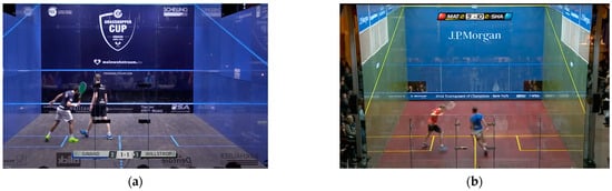
Figure 10.
(a) Data #402, Gawad/Willstrop 2018 Grasshopper 1:02:48 Stroke [23]. (b) Data #92, Matthew/Shabana 2014 Tournament of Champions (ToC) 1:35:10 Yes Let [24].
The above two cases are a great demonstration of how the distance between players can cause the decision to change. In both scenarios, the player location and the ball location are similar, yet the former is decided as a Stroke and the latter as a Yes Let. This is because in the first scenario, the two players are very closely positioned. If the attacking player were going to play the ball, he would likely strike his opponent. Therefore, a Stroke is awarded to the attacking player. In the second scenario, there is more space between the players, and the attacking player would have enough space to hit the ball without hitting his opponent. Therefore, the referees deemed the situation as Yes Let.
3.5.2. Distance of the Attacking Player (AP) to the Ball Position in the Frame
The distance of AP to the ball provides useful information in making decisions. If the ball is close to the AP, there is a greater possibility of the decision being a Stroke; the further the ball is from the AP, the higher the chance is of the decision being a No Let. The distance can be a good indicator of the attacking player’s ability to play the ball. There are lower chances of a No Let if the attacking player is ready to play the ball instead of being on the way to the ball—see Figure 11.
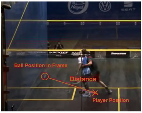
Figure 11.
Data #4, Gaultier/Elshorbagy 2014 ElGouna 19:57 YesLet [17].
However, the ball position is not necessarily a good indicator of where the player will play the ball. In situations where the ball travels to the back of the court and the interference happens when the ball is in the middle, the distance of the AP to the ball can provide information about where the player will play the ball. In situations where the ball is travelling to the front of the court, the distance of the AP to the ball can be misleading because the ball position in the frame will travel towards the player and end at the second bounce position. In this case, where the player will play the ball is closer to the player than the ball position in the frame, and the distance of the AP to the ball is exaggerated—see Figure 12.
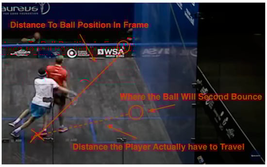
Figure 12.
Data #39, Matthew/Elshorbagy 2014 British Open 49:11 Yes Let [25].
The above situation is a case in which this information can be a useful tool, as the ball position in the frame is close to where the player is going to play it. The distance therefore provides insights into the player’s ability to reach the ball.
This situation is a case in which this information can be misleading. The ball is travelling towards the attacking player; therefore, the ball position in the frame is significantly further than the distance the attacking player actually has to travel.
3.5.3. Distance of the Retreating Player (RP) to the Ball Position in the Frame
The distance of the retreating player to the ball can provide information about how much the RP is blocking access to the ball. If the RP is far away from the ball, the situation should err away from a Stroke. If the RP is right next to the ball, it shows that the RP is blocking access to the ball, which would push the decision towards a Stroke—see Figure 13.

Figure 13.
Data #25, Gaultier/Elshorbagy 2014 ElGouna 1:42:50 Stroke [17].
Similar to the distance of the AP to the ball position in the frame, this value may not be a good indicator of where the attacking player would play the ball. If the ball position in the frame is next to the RP, but the AP is still too far away to play the ball, the situation can be considered a Yes Let or No Let—see Figure 14. On the other hand, if the ball position in the frame is far away from the RP, but it will eventually end next to the RP, the situation can still be considered a Stroke.
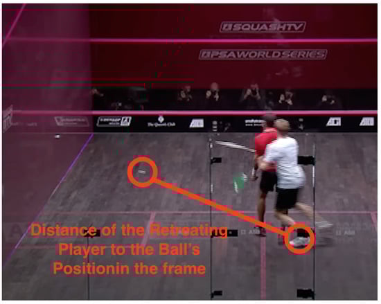
Figure 14.
Data #364, Shabana/Matthew 2013 World Tour Finals 1:00:33 No Let [26].
This example shows how the distance of the RP to the ball can be a good indicator that the situation is a Stroke. In this case, the RP accidentally hits the ball back to himself, and the AP would have hit him had he attempted to swing at the ball. Therefore, because the distance of the RP to the ball is small, this situation is considered a Stroke.
This situation shows that the distance of RP to the ball can also be an indicator if the situation is a No Let. In this case, the RP is very far from the ball, which suggests that the AP created his own interference by moving directly toward the RP, or the AP could not have reached the ball had there been no interference. In either case, the decision would be No Let.
3.5.4. Distance of the Attacking Player (AP) to the Second Bounce
Usually, the referee looks at the second bounce to determine how far away the ball is from the players. By considering the distance of the AP to the second bounce, we can gain information about how far the attacking player has to move before arriving at a position to play the ball. This value can be very straightforward when the ball remains at the front of the court: the closer it gets to the AP, the higher the chance of a Stroke—see Figure 15.
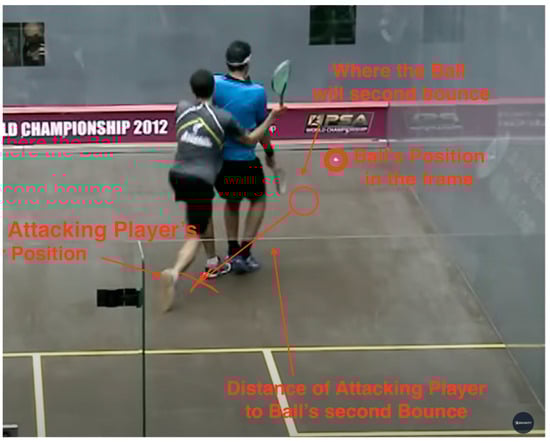
Figure 15.
Data #142, Ashour/Elshorbagy 2012 World Championship 1:30:41 Stroke [27].
However, when the ball travels to the back of the court, at some point it is closest to the attacking player, and then it travels away. Had there been no interference, the attacking player would ideally play the ball when it is closest to him instead of following the ball until its second bounce. In this case, the distance of AP to the second bounce position again fails to identify where the player is going to play the ball—see Figure 16.

Figure 16.
Data #134, Ashour/Elshorbagy 2012 World Championship 1:13:29 Yes Let [27].
In the case above, the distance of the attacking player to the second bounce supports the Stroke decision. Where the ball lands for its second bounce is very close to the AP, which means that the AP could have easily played the shot, had there been no interference. Since the retreating player is directly in the way, this is one of the most obvious Stroke decisions.
This is a case where the distance of the attacking player to the second bounce is an inaccurate representation of the attacking player’s ability to reach the ball. Had there been no interference, the AP would have played the ball around the service box. If we consider the distance to the second bounce, the AP would be unjustly evaluated for his ability to retrieve the ball, since he only has to move to the service box instead of having to move to the back of the court.
3.5.5. Distance of the Racket Head to the Retreating Player (RP)
If the swing of a player is impeded by the other player and they would have been able to play the ball otherwise, a Stroke would be awarded to the player. The distance of the racket head to the retreating player aims to capture this aspect of decision making. If the racket head is close to the retreating player and the ball is close to the AP, the situation likely results in a Stroke—see Figure 17.
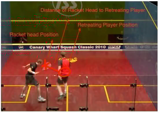
Figure 17.
Data #192, Matthew/Willstrop 2010 Canary Wharf 1:41:18 Stroke [28].
This is an example of the racket head being too close to the retreating player, and the referee deemed the situation a Stroke. Had the AP swung at the ball, the RP would likely have been hit. After all, this distance provides similar information to the distance of the AP to the RP, but we hypothesize that this may provide a more accurate value.
3.5.6. Distance of the Ball Position in the Frame to the Second Bounce
In making decisions, the referee considers the “quality of shot”. If there is interference, yet the shot is “too good”, the referee makes a decision of No Let. This value aims to present information about how good the shot is. The distance of the ball’s position in the frame to the second bounce shows how far the ball has to travel before it “dies”, and therefore indirectly provides information about how much time the player has to retrieve the ball if there is no interference, or the “time remaining”. If the contact happened and the ball died right away, the AP could not have gotten to the ball, even if there was no interference—see Figure 18. On the other hand, if there is still lots of time until the ball dies after the interference, the situation is likely a Yes Let.
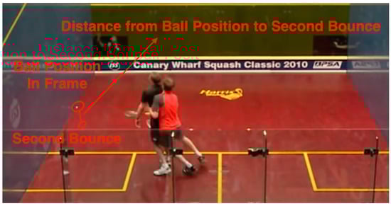
Figure 18.
Data #167, Matthew/Willstrop 2010 Canary Wharf 1:02:50 No Let [28].
This situation demonstrates how this information can be used to determine No Let. As the ball hits the “nick” on the first bounce (the “nick” is the corner between the floor and the wall; when a ball lands in the nick, its energy is dissipated, and it can die very quickly), the ball falls very short, which leaves no time for the AP to retrieve the shot. Because the distance of the ball’s position to the second bounce is short, the referee deemed the situation a No Let, as the AP could not reach the ball even if there was no interference.
3.5.7. Distance of the Racket Head to the Ball Position in the frame
This value provides similar information to the distance of the attacking player to the ball position in the frame. We included this information because sometimes the reach of the player can be long enough to reach the ball even when their body is more than a meter away. The racket head position may provide more useful information about the attacking player’s ability to play the ball than the attacking player’s position—see Figure 19.
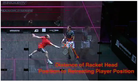
Figure 19.
Data #214, Shabana/Gaultier 2011 World Series Finals 33:09 Stroke [29].
This case is an example of why the distance of the racket head to the ball position may provide a better notion of the attacking player’s ability to play the ball than the distance of the attacking player to the ball’s position. In this case, the AP’s racket head is very far from his body. He is fully stretched and can strike a ball that is more than one and a half meters away from him. Here, simply calculating the distance of the AP to the ball may provide a false sense that the AP is still some distance away from the ball. Therefore, we decided to include this value.
3.5.8. The Shortest Distance from the Racquet Head to the Path of the Ball
For multiple of the values described above, the limitation of “not being able to identify where the AP is going to play the ball” exists. This value aims to resolve this issue by calculating the shortest distance from the path of the ball to the AP’s racket head. The path of the ball is defined as the straight line segment from the ball’s position in the frame to the second bounce position. We define the shortest path to be the line which originates from the racket head’s position and is perpendicular to the ball’s path. If the line intersects the ball path (as the ball path is a line segment and could end before the intersection happens), we calculate the distance from the racket head position to the intersection. If an intersection does not exist on the line segment, we take the closest ending point (either second bounce or ball position) on the line segment and calculate the distance from it to the racket head’s position—see Figure 20 and Figure 21.
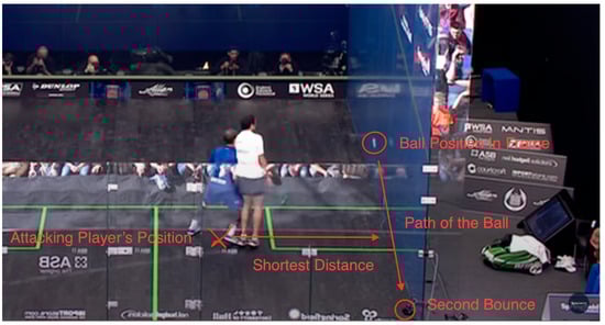
Figure 20.
Data #283, Gaultier/Ashour 2013 British Open 22:55 Yes Let [30].

Figure 21.
Data #390, Farag/Coll 2019 British Open 1:05:40 Yes Let [31].
This is an example of the shortest distance to the ball’s path. If there was no interference, the AP would have chosen to approach the ball through the path with the shortest distance (which is the line perpendicular to the path) instead of travelling all the way to where the ball bounces.
In this case, the shortest distance to the path of the ball is the distance to the second bounce position. Because the perpendicular line to the ball’s path originating from the AP’s position does not intersect with the line segment (does not exist on the path), we took the closest ending point of the segment (either ball position in the frame or second bounce position) as the closest point.
3.5.9. Access to the Front Wall: How Much Is Blocked by the Other Player
When the RP blocks the AP’s access to the front wall, the situation is considered a Stroke. This rule is sometimes compromised when the blockage is minor or the AP is not able to make a shot due to the speed or the position of the ball. Although this is not a clear-cut situation, a significant blockage of the front wall is still considered a Stroke. We calculated the blockage by drawing lines from the AP to both sides of RP, offset by the player’s body width, and analyzing where the lines meet the front wall—see Figure 22. For this study, we defined the body width as 80 cm, as the average shoulder width for men is around 40 cm, and we added 40 cm of width to the total width due to the arms and the legs on each side [32].
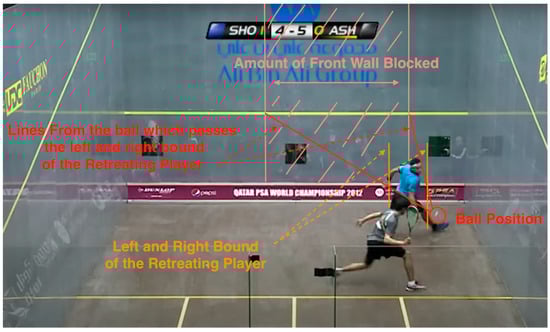
Figure 22.
Data #118, Elshorbagy/Ashour 2012 World Championship 23:16 Stroke [27].
This is an example of how the amount of blockage on the front wall is calculated. Two imaginary lines were drawn from the ball passing the bounds of the RP and reaching the front wall. The final blockage was the width of the area (labeled in pink) inside the two lines.
4. Results
4.1. Results with Mathematica
4.1.1. Experimental Design
When using Mathematica, out of the 400 decisions, 60 decisions were taken out as the test set and 340 remained as the training set. The dataset was shuffled before the test set was taken out. As the dataset was small in number and each shuffle may have caused big percentile changes to the testing set, every experiment was performed five times to obtain a better understanding of the average model performance.
We used the built-in functions provided by Mathematica, namely the Classify function through the application of neural networks [33].
4.1.2. Model Performance on Primitive Data Components
Training on All Six Data Components
Overall, the five runs displayed an average accuracy of 81.4% ± 8.36%—see Figure 23. The accuracy varies drastically over the five runs. The highest accuracy reached 95%, and the lowest fell to 70%. Over the five runs, the distribution of the randomized data is relatively consistent: 8 No Lets, 33 to 36 Yes Lets, and 16 to 19 Strokes. The models are able to accurately classify Yes Lets and are relatively able to accurately classify Strokes. Most models struggle with classifying No Lets.
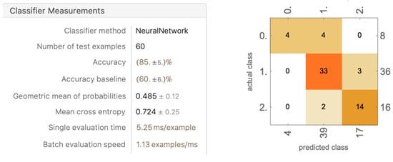
Figure 23.
A trial of the five models trained on all six data components (for the remaining four trials, see Appendix A).
It is worth noting, in every model, that the number of No Lets being classified as Strokes and Strokes being classified as No Lets is mostly zero, with the greatest number not exceeding two. This shows that there is, in fact, a clear divide in Strokes and No Lets, and such a difference can be detected with the neural network.
Dropping Out Data Components
As only the positional values are inputted, some values may act as noise in the model and, in fact, cause the model to perform worse. We kept the AP position, the RP position, and the ball position in the frame, then investigated the effect of dropping out combinations of the remaining values.
Dropping out Racket Head Position
The result of dropping out the racket head position yielded an average accuracy of 82.6% ± 5.89%—see Figure 24. The accuracy improved by 1%, and the standard deviation reduced by nearly 3%. Over the runs, the randomized dataset was less stable than when trained using six parameters, with more fluctuations in the amount of each decision. The Yes Lets and Strokes were still classified with accuracy, and the No Lets were classified with more consistent accuracy. These results confirm the hypothesis that the model may perform better after dropping out some data components. The rationale behind this scenario is potentially that the racket head position provides similar information to the AP position, just offset by the reach of the player. Thus, having similar information with noise may not help the model after all.
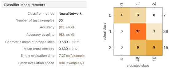
Figure 24.
A trial of the five models trained with dropping out racket head position (for the remaining four trials, see Appendix B).
Dropping out Racket Head Position and the First Bounce Position
Removing the information on the first bounce position drastically decreased model performance to an average accuracy of 71.6% ± 5.82%—see Figure 25. The model became more inconsistent in every category compared to the result of only dropping out racket head position. The first bounce position was removed, as we hypothesized that the ball position in the frame and the second bounce could provide enough information about the ball’s path, and the first bounce position, sometimes located in front of the ball position in the frame and sometimes located behind, only provides noise. This hypothesis was proven wrong, as the first bounce position does play an important role in predicting decisions.

Figure 25.
A trial model trained with dropping out racket head position and the first bounce position (for the remaining 4 trials, see Appendix C).
Dropping out Racket Head Position and Second Bounce Position
The models trained with these sets of data components performed the worst of all, with the average accuracy falling below 69% ± 1.79%—see Figure 26. The rationale behind taking away the second bounce is that, in all interferences, the contact occurred before the second bounce, and in many interferences, the second bounce traveled away from the position of contact, which may have caused it to be less valuable as an informational data component. However, this notion was proven wrong, as the accuracy fell below 70% and became inconsistent in all categories.
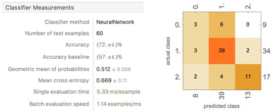
Figure 26.
A trial model trained with dropping out racket head position and the second bounce position (for the remaining 4 trials, see Appendix D).
4.1.3. Model Performance with Modified Data Components
The nine modified data components are as follows:
- Distance of the Attacking Player (AP) to the Retreating Player (RP)
- Distance of the Attacking Player to the Ball’s Position in the frame
- Distance of the Retreating Player to the Ball’s Position in the Frame
- Distance of the Attacking Player to the Second Bounce
- Distance of the Racket Head to the Retreating Player
- Distance of the Ball’s Position in the frame to the Second Bounce
- Distance of the Racket Head to the Ball’s Position in the frame
- The Shortest Distance From the Racquet Head to the Path of the Ball
- Access to the Front Wall: How Much is Blocked by the Other Player
We proposed training a model using this second layer of information to assess whether it improves performance. Considering that among these nine pieces of information, some may contain redundant information, we trained several models with selected values and compared their performances.
All Nine Modified Data Components (MDCs)
In this experiment, we used all nine MDCs to train the model. A total of 340 decisions were used in the training set, and 60 were used in the testing set—see Figure 27.
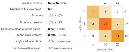
Figure 27.
A trial model trained on all nine modified data components (for the remaining four trials, see Appendix E).
The average accuracy reached 86% ± 3.03%. This performance was the best achieved yet through Wolfram Mathematica. Compared to the previous best model achieved by dropping out racket head position, the average accuracy improved by 3.4% and the standard deviation decreased by 2.86%
Including Modified Data Components (MDCs) #1, #2, #3, #4, #6, #8, #9
In the second experiment, we excluded MDC #5 and MDC # 7, as we believe that they can be redundant to some of the other values—see Figure 28. MDC #5, “Distance of the Racket Head to the Retreating Player”, provides similar information to MDC #1, “Distance of the Attacking Player to the Retreating Player”. MDC #7, “Distance of the Racket Head to the Ball’s Position in the frame”, provides similar information to MDC #4, “Distance of the Attacking Player to the Second Bounce”.

Figure 28.
A trial model trained on seven modified data components (for the remaining four trials, see Appendix F).
The average accuracy dropped to 81.2% ± 6.625%. This indicates a failed attempt to remove information. The standard deviation also drastically increased. Some trials reached an accuracy of 90%, yet some dropped to 73%. Overall, the results were inconsistent, and the accuracy dropped.
Including Modified Data Components (MDCs) #1, #2, #3, #4, #6
In our third experiment, MDC #8 and MDC #9 were also removed. Those two values are two special cases because, in the process of calculating these values, complicated methods were used (see Section 3.5.8 and Section 3.5.9). All other values were determined simply by finding the distance between positions. In removing those two values, we wanted to assess how much they contributed to the model’s performance—see Figure 29.
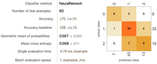
Figure 29.
A trial model trained on five modified data components (for the remaining four trials, see Appendix G).
The model performance reached an average accuracy of 78.8% ± 5.84%. This value is more than 7% lower than when all nine MDCs are used and 2.4% lower than when only MDCs #5 and #7 are removed. This indicates that those two values indeed contain useful information for the model’s performance.
4.1.4. Model Performance with Modified Data Components Combined with Primitive Data Components
In this section showing the Wolfram Mathematica results, we explored the performance of our model when trained with two sets of data components: the modified data components (MDCs) and the primitive data components (PDCs). The idea is that although the distance-related data components, which are the modified ones, can provide good insights into what the situation is, the model could not understand the location of where on the court this all happened. Therefore, by combining the position-related and distance-related data components, we can build a more well-rounded model, which hopefully will improve its performance.
In total, 21 data components were taken into consideration (12 primitive and 9 modified). In this section, combinations of each are tested. All PDCs and MDCs are listed here.
PDCs:
- 1 and 2: Attacking Player Position X and Y Value
- 3 and 4: Retreating Player Position
- 5 and 6: Ball Position in the frame
- 7 and 8: First Bounce
- 9 and 10: Second Bounce
- 11 and 12: Racket Head Position
MDCs:
- Distance of the Attacking Player (AP) to the Retreating Player (RP)
- Distance of the Attacking Player to the Ball’s Position in the frame
- Distance of the Retreating Player to the Ball’s Position in the frame
- Distance of the Attacking Player to the Second Bounce
- Distance of the Racket Head to the Retreating Player
- Distance of the Ball’s Position in the frame to Second Bounce
- Distance of the Racket Head to the Ball’s Position in the frame
- The Shortest Distance from the Racquet Head to the Path of the Ball
- Access to the Front Wall: How Much is Blocked by the Other Player
Training with all 21 Data Components
In the first experiment, we utilized all data components that we had. All 21 data components are fed into the model, and we investigated the model performance—see Figure 30.
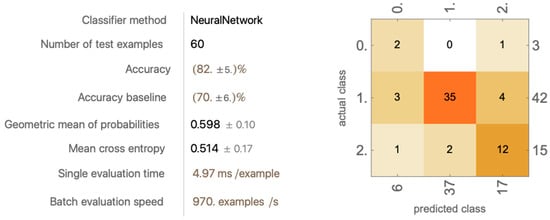
Figure 30.
A trial model trained on all 21 data components (for the remaining four trials, see Appendix H).
The model’s accuracy dropped to 81.8% ± 3.71%. Surprisingly, the model performance did not improve after combining the PDCs and the MDCs. One possible explanation for this is that too many data components were provided for a small dataset. The model is incapable of learning all the correlations using the resources it has.
Training with Primitive Data Components (PDCs) #1–10 and All Modified Data Components (MDCs)
As shown in previous experiments, PDCs #11 and 12 (racket head position) acted as noise in the model. In this experiment, we excluded these two values and evaluated the model performance—see Figure 31.
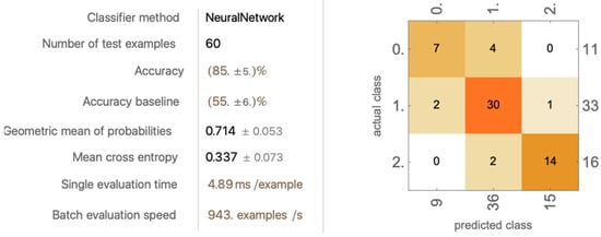
Figure 31.
A trial model trained on primitive data components #1–10 and all modified data components (for the remaining four trials, see Appendix I).
The average accuracy as 82.2% ± 6.68%. No significant improvements were observed after these values were removed.
Training with Primitive Data Components (PDCs) #1–10 and Modified Data Components (MDCs) #3, #5, #6, #8, and #9
In this experiment, we selected certain MDC values and evaluated model performance—see Figure 32.
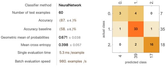
Figure 32.
A trial model trained on primitive data components #1–10 and five modified data components (for the remaining four trials, see Appendix J).
The average accuracy reached 84.8% ± 6.17%. No significant improvements were observed after some values were removed.
4.2. Results with Python
4.2.1. Experimental Design
When using Python, slightly different from the method applied when using Wolfram Mathematica, the 400 decisions were split into three sections: 280 (70%) in the training set, 40 (10%) in the validation set, and 80 (20%) in the testing set. The neural network consisted of two layers with 64 nodes and 128 nodes, and one output layer.
In the training process, the Pandas package was used to read the dataset. The Scikit-learn package was used to shuffle the dataset. The TensorFlow package was used to modify the data and train the neural network.
4.2.2. Model Performance on Primitive Data Components
Training on All Six Data Components
The models trained with all six data components (as shown in Table 1) performed significantly worse than their Wolfram Mathematica counterparts, achieving an average accuracy of 0.747 ± 0.022 and an average loss of 0.717 ± 0.034. With Wolfram Mathematica’s built-in neural network training method unavailable, it was hard to replicate the results achieved by Wolfram Mathematica.

Table 1.
Five trials of the model trained on all six data components.
Dropping Out Data Components
Although it is hard to replicate the results achieved by Wolfram Mathematica, the same drop-out method could be tested on the neural network. The core data components of AP position, RP position, and the ball’s position in the frame were kept, and the remaining three were dropped to test if this method increased the performance of the model—see Table 2, Table 3, Table 4 and Table 5.
Table 2.
Five trials of the model trained by dropping out the racket head position.
Table 3.
Five trials of the model trained by dropping out racket head position and second bounce position.
Table 4.
Five trials of the model trained by dropping out racket head position and first bounce position.
Table 5.
Five trials of the model trained by dropping out racket head position, first bounce position, and second bounce position.
The model that achieved the best accuracy was that trained on the dataset which dropped out the racket head position and first bounce position, with an average accuracy of 78.3% ± 1.6%, being around 4% less accurate than the best model trained in Wolfram Mathematica.
4.2.3. Model Performance and Normalization
Taking the best model (trained on dropping out the racket head position and first bounce position), we investigated the effect of normalization on this task. The above results were all performed by models trained with data normalized by TensorFlow’s built-in normalization function. We trained models five more times without normalization to observe the result—see Table 6.
Table 6.
Five trials of the model trained without normalization.
The average accuracy dropped by around 7% with a similar average loss. This result demonstrates that the normalization method helped the model during the classification process.
4.2.4. Model Performance with Modified Data Components
The nine modified data components are as follows:
- Distance of the Attacking Player (AP) to the Retreating Player (RP)
- Distance of the Attacking Player to the Ball’s Position in the frame
- Distance of the Retreating Player to the Ball’s Position in the frame
- Distance of the Attacking Player to the Second Bounce
- Distance of the Racket Head to the Retreating Player
- Distance of the Ball’s Position in the frame to Second Bounce
- Distance of the Racket Head to the Ball’s Position in the frame
- The Shortest Distance from the Racquet Head to the Path of the Ball
- Access to the Front Wall: How Much is Blocked by the Other Player
We proposed training a model using this second layer of information to assess it would improve our model performance. Considering that among these nine pieces of information, some are perhaps redundant, we trained several models with selected values and compared their performances.
All Nine Modified Data Components (MDCs)
In the first experiment of this section, we decided to use all nine values to train the model. The experimental parameters were kept the same, with 280 decisions in the training set, 40 in the validation set, and 80 in the testing set. The neural network still consisted of two layers with 64 nodes, 128 nodes, and 1 output layer—see Table 7.
Table 7.
Five trials of the model trained with all nine modified data components.
Our model reached an accuracy of 80.5% ± 3.0%. This result exceeded the previous best model achieved in Python by around 1.7% on average. The average loss drastically decreased by more than 15%. This indicates that the modified data approach may indeed be useful to the model training process.
Including Modified Data Components (MDCs) #1, #2, #3, #4, #6, #8, #9
In the second experiment, we excluded MDC #5 and MDC # 7. These two values were excluded as we believe they may be redundant to some of the other values. MDC #5, “Distance of the Racket Head to the Retreating Player”, provides similar information to MDC #1, “Distance of the Attacking Player to the Retreating Player”. MDC #7, “Distance of the Racket Head to the Ball’s Position in the frame”, provides similar information to MDC #4, “Distance of the Attacking Player to the Second Bounce”—see Table 8.
Table 8.
Five trials of the model trained with seven modified data components.
The average accuracy increased by 0.5%, indicating that this was a successful attempt at removing information. The average loss stayed around the same value, increasing by 6%.
Including Modified Data Components (MDCs) #1, #2, #3, #4, and #6
In our third experiment, MDC #8 and MDC #9 were removed. These two values are special cases, because in the process of calculating them, complicated methods were used (see Section 3.5.8 and Section 3.5.9). All other values were calculated by finding the distance between positions. In removing these two values, we wanted to assess how much they contributed to model performance—see Table 9.
Table 9.
Five trials of the model trained with five modified data components.
Surprisingly, the model accuracy did not drop compared to using all nine data components. The model also had a lower and comparatively more stable standard deviation. This might indicate that MDCs #8 and #9 do not provide useful information.
4.2.5. Model Performance with Modified Data Components Combined with Primitive Data Components
In this section showing the Python results, we explored the performance of our model when trained with two sets of data: the modified data components (MDCs) and the primitive data components (PDCs). In total, 21 data components were taken into consideration (12 primitive and 9 modified). In this section, combinations of each are tested. All PDCs and MDCs are listed here.
PDCs:
- 1 and 2: Attacking Player Position X and Y value
- 3 and 4: Retreating Player Position
- 5 and 6: Ball Position in the frame
- 7 and 8: First Bounce
- 9 and 10: Second Bounce
- 11 and 12: Racket Head Position
MDCs:
- Distance of the Attacking Player (AP) to the Retreating Player (RP)
- Distance of the Attacking Player to the Ball’s Position in the frame
- Distance of the Retreating Player to the Ball’s Position in the frame
- Distance of the Attacking Player to the Second Bounce
- Distance of the Racket Head to the Retreating Player
- Distance of the Ball’s Position in the frame to Second Bounce
- Distance of the Racket Head to the Ball’s Position in the frame
- The Shortest Distance from the Racquet Head to the Path of the Ball
- Access to the Front Wall: How Much is Blocked by the Other Player
Training with all 21 data Components
In the first experiment, we utilized all data components we had. All 21 data components were fed into the model, and we investigated the model performance—see Table 10.
Table 10.
Five trials of the model trained with all 21 data components.
This model achieved the highest accuracy yet in the Python section, exceeding the previous best Python model by 2.7%. This proves the idea that positional data components, adding to the distance-related data components, can improve the model’s understanding of interferences and thereby boost performance.
Training with Primitive Data Components (PDC) 1–10 and All Modified Data Components (MDCs)
As shown in previous experiments, PDCs #11 and 12 (racket head position) could act as noise in the model. In this experiment, we excluded those two values and evaluated the model performance—see Table 11.
Table 11.
Five trials of the model trained with primitive data components #1–#10 and all modified data components.
In this experiment, the average accuracy was again considerably improved by around 1.5% compared the model trained in the previous experiment. It is currently the model with the best accuracy in the Python section. It is worth noting that the fifth trial provided the current best singular trial model in Python, with 91.2% accuracy.
Training with Primitive Data Components (PDCs) #1–10 and Modified Data Components (MDCs) #3, #5, #6, #8, and #9
In this experiment, we selected certain MDC values and evaluated model performance—see Table 12.
Table 12.
Five trials of the model trained with primitive data components #1–10 and five modified data components.
Compared to the last model, this model achieved 85% accuracy (within 0.2% of the last model), with far better loss. The loss is 12% lower than in the previous model with a far steadier standard deviation.
5. Discussion
5.1. Analysis of Result
In this section, we analyze the results we found in this study. We compare the best results from both Python and Mathematica.
5.1.1. Overall Result
Overall, the best Wolfram Mathematica model displayed an average accuracy of 86% ± 3.03%, whereas the best Python model demonstrated an average accuracy of 85.2% ± 5.1%.
An average accuracy of 85% already reaches the level of satisfaction in a real-life setting (further explanation see Section 5.1.3). For instance, in a regular professional match, the number of calls can vary between 20 and 30. If 85% of the decisions are made correctly, this means that there are three to five incorrect decisions. Given that, in many cases, an interference can be called either way (No Let or Yes Let, Yes Let or Stroke), referees nowadays already make many controversial calls in a regular match. It has to be kept in mind that this level of accuracy is achieved with only 400 referee decisions in our limited, unbalanced dataset. Thus, with proper resources, the potential of machine learning for refereeing the sport of squash is very high and promising.
In is worth noting that for the best-performing models on both platforms, the standard deviation of performance throughout the five trials (3.03% for python, 5.1% for Mathematica) is not large enough to be concerning. Although the standard deviation varies for other models, this is likely a result of data reshuffling and general dataset imbalance. Again, this issue should likely be resolved by sizing up the dataset in our future research.
On the other hand, although the best Wolfram Mathematica and Python models have similar average accuracies, they were trained using drastically different data components. In Wolfram Mathematica, the best model was achieved using only the nine modified data components. In Python, the best model was achieved using both the nine modified data components (MDCs) and the primitive data components (PDCs) #1–10. This result indicates that models trained on different platforms can vary in performance even when using the same data components. Interestingly, Wolfram Mathematica models dropped in accuracy when both PDCs and MDCs were used, but Python models peaked using these sets of data components. To explain this difference, one would have to more deeply examine the structure of neural networks on the two platforms. One feature that has proven very helpful in Wolfram Mathematica is the statistical analysis it provides: accuracy with standard deviation, accuracy baseline, geometric mean of probabilities, and mean cross entropy. Those evaluations are proven to be insightful and truly assist in the fine-tuning process.
Through the accuracy achieved by models on both platforms, we can see that using machine learning to make squash referee decisions is a highly desirable solution to many problems. Machine learning models are objective in nature and would always produce the same decision for the same interference, whereas human referees are prone to outside factors like crowd and player influence. In addition, machine learning models can be more economical to implement.
5.1.2. Usefulness of Different Data Components
To some extent, this study is an investigation into how different combinations of data components contribute to the model performance. Different combinations cause the models to perform differently, and their effects vary between the Wolfram Mathematica section and the Python Section.
The six primary data components (PDCs) already provide enough information for the model to perform at an acceptable level. Using only the six PDCs, the Wolfram Mathematica models reached an average accuracy of 81.4% ± 8.36%, whereas the Python models reached a lower average accuracy of 74.7% ± 2.2%.
The initial drop-out method removes different data components and evaluates the impact of these data components being removed. For Wolfram Mathematica, the accuracy increased to 82.6% ± 5.89% after the racket head position was removed. The accuracy drastically dropped after any other values were removed. For Python, the accuracy increased the most when both the racket head position and the first bounce position were removed, reaching 78% ± 1.6%. The increase in performance after the removal of data components indicates that for the initial six data components, some contain information that could act as noise and prevent the model from improving.
Then, the nine modified data components (MDCs) were introduced to the dataset. We conducted one round of experiments using only the nine MDCs and evaluated the models. Wolfram Mathematica’s models provided the best performance at this stage, reaching an average accuracy of 86% ± 3.03%. The Python models also experienced an increase in performance, reaching an average accuracy of 80.5% ± 3.0%. This shows that the nine MDCs do, in fact, provide useful information, and we were right in calculating them.
As some MDCs are slightly redundant, we experimented with data component drop-out with the nine MDCs. In the first round, MDCs #5 and #7 were removed. This dropped the Wolfram Mathematica models’ average accuracy to 81.2% ± 6.625% but increased the Python model’s average accuracy to 81.0% ± 2.4%. In the second round, MDCs #8 and #9 were removed to evaluate their usefulness to our model, and for both platforms, the accuracy decreased, indicating that those two values are helpful to the model’s performance.
We then combined the MDCs and the PDCs to conduct a final round of evaluation. In this section, only the Python models gained accuracy and better performance. When all MDCs and PDCs were used, the Python models achieved an average accuracy of 83.7% ± 1.4%. When all MDCs and PDCs #1–#10 were used, the Python models achieved their best performance, with an average accuracy of 85.2% ± 5.1%. Another combination of data components using MDCs #3, #5, #6, #8, #9 and PDCs #1–#10 reached an average accuracy of 85.0% ± 2.4%, with a 15% smaller loss and far steadier standard deviation compared to the best-performing model.
5.1.3. Estimation of Real-Life Referee Accuracy
Although the accuracy of human referees in squash is not published in peer-reviewed literature, it can be estimated fairly accurately. First, as Bordner observes,
“Baseball umpires are, by the most optimistic estimates, only 90% accurate in calling balls and strikes. While this might sound impressive, we only know this because of the already-99%-accurate Pitchf/x system Major League Baseball uses in every ballpark to evaluate its umpires. Moreover, the 9% difference in accuracy between human umpires and Pitchf/x is enormous … And as determinations of sporting facts go, ball-strike calls are relatively simple: the umpire, from a static position, need only track one object moving directly toward him/her with the plate and the batter’s stance to help indicate the strike zone. Things are much more complicated and difficult in other sports …”[34]
Second, the estimate of 90% accuracy for human refereeing in baseball is further confirmed by Williams [35]. Third, as Bordner [34] observes in the above quote, refereeing in baseball is much simpler than in other sports, especially in squash, which is known to be particularly highly stressful for referees [36]. Fourth, the anecdotal opinion of squash players, coaches, and referees is that there are two to three controversial calls per game. With, say, 20 points in the game, this leads to an accuracy estimate of 3/20 = 85%, which is lower than the accuracy in baseball, as it should be. Finally, the top competitive players confirm our estimate of up to 85% accuracy in human refereeing of squash [37].
5.2. Case-by-Case Analysis of Some Wrong Calls
In this section, we perform a case-by-case analysis of incorrectly made decisions. We take two of each kind of incorrect decision made by our models and provide reasons for why they might be incorrectly called in the model and real-life perspectives. We hope that in doing this, we can find some insights regarding why the model made the wrong calls.
The incorrect decisions are made by the best-performing models in Python. We chose models trained in Python for this section because the prediction results were easier to fetch, and the Python best-performing model was trained using PDCs #1–#10 and all MDCs. Thus, almost all data components were considered.
5.2.1. Yes Lets Classified Incorrectly
Figure 33 and Figure 34 show situations where the model has given an incorrect referee deci-sion to an originally “Yes Let” call. The figures are followed by detailed analysis of what may have caused the issue.

Figure 33.
Data #144, Matthew/Willstrop 2010 Canary Wharf 8:39 Yes Let [28]. Possibility given by model: [No Let—94%, Yes Let—6%, Stroke—0%].
Figure 34.
Data #347, Matthew/Gaultier 2018 ToC 1:32:33 Yes Let [38]. Possibility given by the model: [No Let—0%, Yes Let—43%, Stroke—57%].
In this situation, the RP played a ball that died very quickly. The AP was provided a line to the ball. The referee deemed this situation a Yes Let, as interference occurred and he thought that the AP could get the ball. From our perspective (as a non-professional normal viewer biased by our experiences), this could also be identified as a No Let, as the ball’s quality is high, and the AP may not successfully reach the ball even without the interference.
The model deemed this more likely a No Let, possibly because the ball fell short. It is worth noting that the possibility it provided is overwhelmingly in favor of the No Let decision, which is likely incorrect. The possibility for No Let should not reach more than 90%, as this case would represent a close call.
This case, in fact, is a controversial one in itself. The RP played a ball that landed very close to him, yet the referee thought there was enough distance away from it to consider the situation a Yes Let. In the video, the commentators pointed out that it is possible to consider this a Stroke:
“Well, I mean eh, it’s not the best of shots here from Matthew (the RP). This is going to be interesting, Massarella (the referee) is gotta be consistent… If you watch where the ball bounces, the second bounce is by the service line…. Well, I can assure you that Gregory Gaultier (the AP) will not be taking John Massarella out for any type of food or beverage… I think that was a stroke”.[38]
Similar to the commentators, we think that this should have been called as a Stroke, because the ball bounced right back to the RP, and the RP was not able to clear. Our model agreed with us by assigning a 57% possibility to Stroke. This provides a good example of how human referees can make controversial decisions that the commentators and the audiences disagree with.
5.2.2. No Lets Classified Incorrectly
Figure 35 and Figure 36 show situations where the model has given an incorrect referee decision to an originally “No Let” call. The figures are followed by detailed analysis of what may have caused the issue.
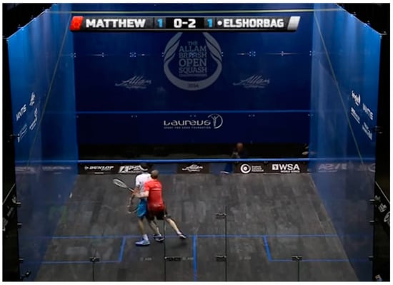
Figure 35.
Data #46, Matthew/Elshorbagy 2014 British Open 1:03:19 No Let [25]. Possibility given by model: [No Let—6%, Yes Let—93%, Stroke—0%].

Figure 36.
Data #333, Matthew/Gaultier 2018 ToC 36:22 No Let [38]. Possibility given by model: [No Let—32%, Yes Let—68%, Stroke—0%].
This is not a very controversial decision. The RP’s shot went backward and was very close to the side wall. Although the AP could have possibly retrieved it had the RP not been there, the AP first went the wrong way (forwards) as he was deceived by the shot. The AP also showed very little effort to travel through the interference and play the ball. The AP took the “wrong path” to the ball, combined with the quality of the shot from the RP and the AP’s lack of effort, which is why the referee deemed this a No Let.
Since our model has not learned the idea of a “wrong path” and “effort”, it makes sense that it is unable to understand this situation. From the same position shown in the picture, if the AP took the “right path”, which is left and backward around the RP, this could have well been called a Yes Let.
This case is a situation between a Yes Let and a No Let. The referee deemed the AP unable to reach the shot as the shot quality was “too good”.
In our opinion (as non-professional normal viewers biased by our experiences), this could have been decided either way. Personally, we think that the AP might have been able to reach the ball had the RP provided a path. Therefore, this could have been called as a Yes Let. The commentators and the referee think the opposite because the ball’s quality was very good.
Our model, in fact, reflects our thinking by only assigning a 32% possibility to No Let. This means that according to the model, this could possibly qualify as a No Let as well, although the model leans more towards a Yes Let.
As our model is only trained with 59 cases of No Let, this limits the amount of knowledge it is able to absorb, and it makes sense that our model is still unable to offer the most accurate level of refereeing.
5.2.3. Strokes Classified Incorrectly
Figure 37 and Figure 38 show situations where the model has given an incorrect referee decision to an originally “Stroke” call. The figures are followed by detailed analysis of what may have caused the issue.
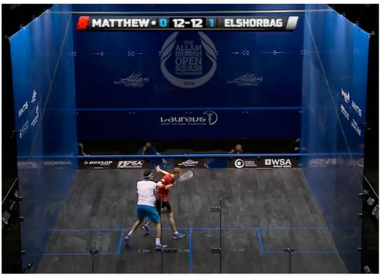
Figure 37.
Data #46, Matthew/Elshorbagy 2014 British Open 58:10 Stroke [25]. Possibility given by model: [No Let—0%, Yes Let—53%, Stroke—47%].
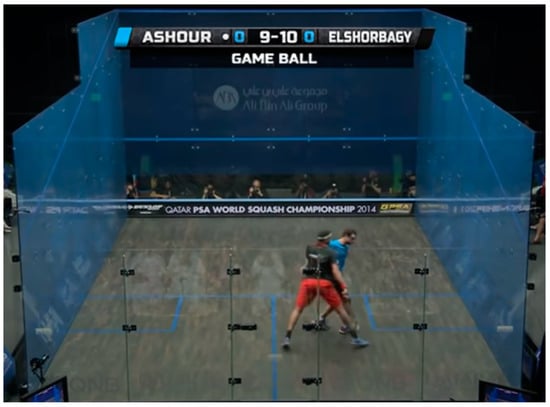
Figure 38.
Data #244, Ashour/Elshorbagy 2014 World Championship 12:08 Stroke [39]. Possibility given by model: [No Let—0%, Yes Let—51%, Stroke—49%].
This is a very interesting case. The AP here is actually “fishing” for a Stroke. This means that the AP is manipulating his body position and exaggerating his swing to make the situation look more like a Stroke than a Yes Let. In this case, the AP stood his ground and waited for the ball instead of looking to play it normally. If the AP was going to play it normally, he would step toward the ball and strike. Since he decided to fish for a Stroke, he shaped up and waited until the ball came to him, as if he were going to hit the ball from where he was. This pushed the striking spot further back, which brought the RP into the range of the AP’s swing. This, combined with the AP’s exaggerated swing, makes the situation look more like a Stroke. In reality, when the ball reached him, it had already bounced twice, so he could have not hit it from where he was.
The commentators noted on the AP’s actions: “He (the AP) is looking for Shorbagy (the RP) there…Well, he’s got it (the Stroke), he is playing the rules…He (the AP) doesn’t usually do that, he doesn’t usually exaggerate. He is doing that (exaggerating his swing)” [25].
In this case, the referee gave a Stroke, although the AP was somewhat fishing for it. To our understanding, the AP’s fishing actions changed the situation from a 50% Stroke to a 70% Stroke.
Our model deemed this as almost a fifty–fifty situation. Of course, there is no knowledge that informs the model that the AP is fishing for a Stroke. It makes sense that our model leans slightly towards a Yes Let call.
This is a pretty clear Stroke. The AP’s swing was prevented by the RP, and the ball was moving right into the AP’s range of swing. The model made the wrong decision, possibly because the ball was at the front of the court when the interference happened, but it did not know that the ball was traveling really fast, and it entered AP’s range when the interference was still happening.
The model provided a 51% to 49% chance in favor of a Yes Let. These are two close possibilities, and with a slight change in one data component, this is possible to overturn to a Stroke. This shows that our model is not far off in its calls.
5.3. Novel Contributions of this Study
Our study is the first one to investigate the process of squash referee decisions and its implications. It is also the first to propose the use of machine learning as a resolution to refereeing discrepancy in the sport of squash. Our proposals regarding the data collection method and the usage of data points are novel along with many detailed analyses of case-specific professional squash decisions. In the process of data collection, we created the first dataset of refereeing decisions in squash.
6. Limitations
6.1. Limitations in the Data Collection Process
6.1.1. Dataset Is Too Small and Imbalanced
The main limitation of this study is the limited size of the dataset. As there is no available dataset for squash refereeing decisions, we had to build our own. Due to the limited time and resources, only 400 data points were collected. With 243 Yes Lets but only 59 No Lets and 98 Strokes, this dataset is also imbalanced. With more data to collect in the near future, our model is very likely to improve its performance.
6.1.2. Speed and Height of the Ball
In our data collection process, we did not collect data components related to the speed and the height of the ball. However, these two data components can provide critical information about optimal decisions. With similar positioning and different speed and height of the ball, the decision could change from a Stroke to a No Let.
As shown in Figure 39, two shots can land in the same position, but the implications can differ drastically. The green path is a slow shot that is possibly easy to retrieve, but the purple path is low and hard to retrieve. Without these two pieces of information, our model cannot learn the difference between the green path and the purple path.
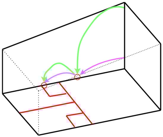
Figure 39.
Illustration of how balls with different speeds and heights can have the same first and second bounce positions.
6.1.3. Assumed All Decisions Are Correct
During our data collection process, we assumed that all decisions we included were correct. However, some of them are still controversial (Data #347, see second example of Section 5.2.1). Our model is thus currently trained on some controversial data, which may have negatively influenced the model’s performance. If this issue is to be resolved, we need more than one squash professional discussing each decision outcome before putting the data into the dataset.
6.1.4. Took in Different Standards of Refereeing
Different referees have different standards of refereeing. Some referees are relatively soft, giving more Yes Lets in ambivalent cases. Some referees are harsh and give more Strokes and No Lets. The data collected for this study came from multiple referees, each having an individual system of refereeing. This leads to some similar cases in our dataset being classified as different decisions. One solution resembles the possible resolution to Section 6.1.3. Assumed All Decisions Are Correct, which is to have several squash professionals decide on one correct decision using one standard of refereeing during the process of data collection.
6.1.5. Different Definition of “Moment”
To collect our data, we defined a “moment”, which is the frame when the players first collide or when the ball first enters the AP’s range of swing. However, the timing of that moment is not always obvious. Therefore, throughout the dataset, there are slight inconsistencies in the picking of moments.
6.1.6. When the Ball Bounces off the Back Wall
When a ball travels a long way and bounces off the back wall, it provides the AP with more time to retrieve it. Most of the time, if the ball bounces off the back wall, the situation is not considered a No Let. In our dataset, we did not put in a measure for when the ball bounced off the back wall. Simply noting the second bounce of the ball does not tell the model if the ball has reached the back wall and bounced back, providing the AP with more time to retrieve the ball.
6.1.7. Time Taken to Clear
A situation could also be decided differently based on how quickly the RP cleared the ball, which means that the RP is no longer preventing the AP from striking the ball. In some extreme cases, the RP can take a very long time or is unable to clear at all—see Figure 40.
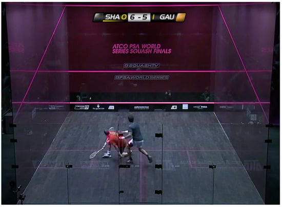
Figure 40.
Data #213, Shabana/Gaultier 2011 World Series Finals 31:11 Stroke [29].
In this case, the AP slipped and fell down. Even though the ball was somewhat far away, the referee deemed this situation a Stroke, because the AP has his path blocked for too long and has absolutely no way to reach the ball by falling down. Had the AP stood still, this situation would probably be considered a Yes Let.
Our model currently does not take clearing time into consideration. To improve on this, more measures should be taken during the data collection process.
6.1.8. Speed and Arm Length of Different Players
Naturally, different players have different speeds and reaches. This is also taken into account when a referee is making decisions. A player who consistently shows his ability to retrieve hard shots may leave an impression of being “fast” to the referee, which potentially makes the referee less inclined to give a No Let to the player.
It is perhaps possible to calculate the speed by analyzing video frames or putting motion sensors into the courts. Previous studies have collected data components such as maximum speed and average speed during squash rallies successfully [15].
6.1.9. Situations of No Appeal
Sometimes, when players think that they are going to receive a No Let decision, they do not appeal at all. From a strategic perspective, appealing and then experiencing rejection disrupts the mentality and flow of one’s game. In our data collection process, we could not take into consideration all of these cases, because even though there was interference, there was not any appeal at all.
These situations are hard to classify, as they are potentially a mistake by the player; the situation may be ruled a Let. In the future, these situations can either be put into the category of No Let or treated as a fourth category of “No Appeal”.
6.1.10. Ability to Further Move
The referees also evaluate a player’s ability to reach the ball based on the player’s ability to further move after the interference—see Figure 41.
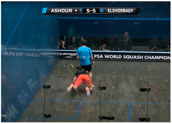
Figure 41.
Data #249, Ashour/Elshorbagy 2014 World Championship 1:06:12 No Let [39].
As an example, this situation was called as a No Let. The AP fell down before the contact happened, so he was not able to further move from this body position. The referee deemed this situation as a No Let because the AP could not have reached the ball, although it was only one step away from him. However, our model does not understand that the AP has fallen and could not take an extra step toward the ball. This is another limitation of this study.
6.1.11. Ability to Make a Shot
Sometimes, even though the ball is within the reach of the AP, the AP’s ability to make a shot is hindered—see Figure 42.
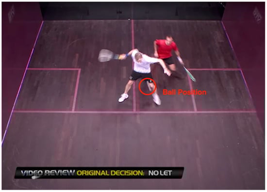
Figure 42.
Not included in dataset, Shabana/Matthew 2013 World Tour Finals 59:30 No Let [26].
In this case, the ball is right in front of the AP, but the AP could not have hit the ball because it went right into him, and his racket could not get into position in sufficient time. To our model, this is a case where the ball is close to the AP and the AP is close to the RP, which means it is possibly a Stroke and is at least a Yes Let. However, in the real-life scenario, the AP is unable to hit the ball, and therefore it is decided as a No Let.
6.1.12. Degree of Interference
Some interferences are heavier than others. Usually, the heavier the interference is, the more inclined the referee is to give a Yes Let or a Stroke because it means that the AP’s ability to reach the ball is taken away to a greater extent—see Figure 43.
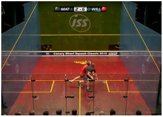
Figure 43.
Data #157 Matthew/Willstrop 2010 Canary Wharf 39:57 Yes Let [28].
This is an example of very heavy contact. The AP fell down after tripping on the RP’s foot. Usually, when the AP is taken out completely in this way, the referee would not issue a No Let, no matter how good the shot is.
Our model has no idea of the degree of interference. To account for this, it is possible to establish a parameter by classifying the degree of each interference based on a scale. This is, however, still an objective case and might not be useful to include in the dataset.
6.2. Limitations Caused by Abstract Refereeing Concepts
6.2.1. Idea of “Wrong Path”
The concept of a “wrong path” is an abstract refereeing concept. To retrieve a shot, the AP should take the quickest path to the ball. If the AP has taken the “wrong path” and is then blocked by the RP, the referees may provide a Yes Let or even a No Let.
This often happens when the AP is first deceived by the shot by the RP and moves the wrong way. When the AP realizes and moves toward the ball from where he finds himself after the initial movement, he is blocked by the RP. The referees sometimes punish the AP for being deceived, in this case by giving a No Let.
6.2.2. Idea of “Accepting Interference”
The concept of “accepting interference” means that the referee deems that the AP travelled through the interference and can play the ball. Thus, if the AP then stops and appeals, the referee would give a No Let—see Figure 44a,b.
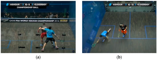
Figure 44.
Data #276, Ashour/Elshorbagy 2014 World Championship 1:21:15 No Let [39]. (a) View taken by the back camera. (b) View taken by the top camera.
In this case, the AP actually travelled through the interference and stopped the ball before the second bounce (the AP usually stops the ball to show they can reach it, and then appeals for a decision). Although the AP showed that he could get it, the referee thought that when he could play the ball, the RP was already away from his swing, and he had “accepted the interference” by going through and reaching the ball. The referee therefore gave a No Let.
This idea of accepting interference varies drastically between different referees. Only referees with harsh standards would impose this concept and give No Lets in this case. Other referees understand that the AP has been impacted on their way to the ball and would give a Yes Let. This remains a controversial idea among referees and audiences.
Our model has no concept of what “accepting interference” is. There is no way to learn that although the AP could have reached the ball, he should have played it.
6.2.3. Idea of “Minimal Interference” and “Lack of Effort”
When the interference is slight and the AP chooses to not play the ball, some referees give a No Let based on the idea of “minimal interference” and “lack of effort”. The referee wants to promote continuous play, which means that the players need to travel through interference that is minimal and show effort that they want to play the ball—see Figure 45.
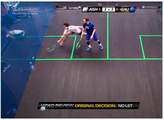
Figure 45.
Not included in dataset, Ashour/Gaultier 2013 British Open 41:08 No Let [30].
In this case, the AP skimmed past the RP, barely touching the RP, and decided to stop the ball and appeal. The referee thought that the AP had shown no effort to play the ball, and therefore gave a No Let. The commentators described the situation in this way:
“We’ve seen Ramy Ashour (the AP) do this, he does actually get to the ball, but there is interference on his way through… Oh, there’s not much interference, minimal there, it’s minimal. So the question for the referee is why doesn’t he go through and play that? There’s not a huge amount of interference. This could stay as a No Let, you know, purely because of lack of effort…He could have clearly played the ball, he elected not to, and he’s paid the price. I think that’s a good decision (No Let)”.[30]
Our model would only know that the AP is close to the ball and could have retrieved the ball. It does not understand that the referee wants to promote continuous play and that those situations should amount to a No Let.
6.2.4. Idea of “Punishment for Bad Shot”, “Going around Opponent”, and “Shut Out”
Some referees believes in the idea of “Punishment for Bad Shot”, “Going around Opponent”, and “Shut Out, ” which is the justification of interference in face of great shot quality. In other words, if the shot played by the attacking player is too good, the referee ignores the physical interference and gives a “No Let” to the retrieving player—see Figure 46.
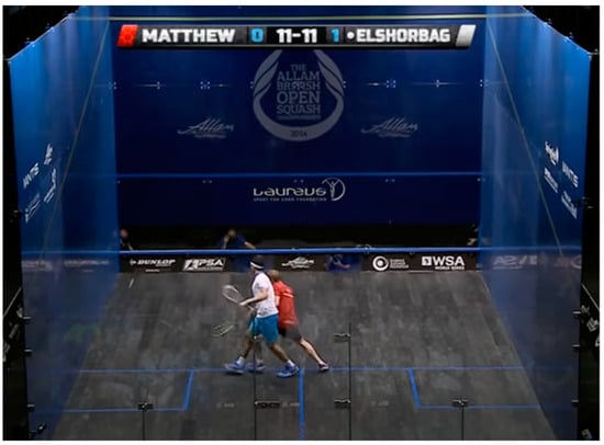
Figure 46.
Data #43, Matthew/Elshorbagy 2014 British Open 55:56 No Let [25].
In this case, the AP’s previous shot was loose and the RP hit a ball straight down the left side wall. The AP tried to reach it but his path was blocked by the RP. The RP has “shut out” the AP. The referee gave No Let and explained “the ball was too good” [25]. Here is what the commentators said:
“He’s taken his space there, Elshorbagy (the RP). Loose shot from Nick Matthew (the AP). Nick Matthew has to go around the back of Elshorbagy if he wants to go and get that ball. (The other commentator) Well, it’s his shot to play, Elshorbagy. Definitely his shot to play. But you also, I mean, this is where you get the middle ground. Because it’s his (the RP’s) shot to play, therefore Matthew needs to go around and play the ball, but then he (the RP) also needs to give access”.[25]
To the commentators, this could be decided either way: either a No Let, because the AP played a loose ball and therefore should receive punishment and go the long way round, or a Yes Let, because the RP did not provide the shortest path to the ball.
This is, in fact, a controversial decision, as the referees’ ideas collide. The RP is not providing a path (shutting the AP out), but the AP has hit a loose shot and has compromised his position on the court to compensate for the bad shot. Some referees think that in this case, it is justified to punish the AP and give a No Let. Some referees believe that because a path is not provided, there is good reason to issue a Yes Let.
6.2.5. Idea of “Not Allowing to Clear”
The idea of “not allowing to clear” describes a situation where the AP holds the RP in position to make the situation look more like a Stroke—see Figure 47.
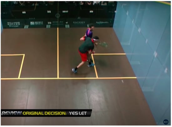
Figure 47.
Data #316, Elshorbagy/Ashour 2014 World Series Finals 37:47 Yes Let [40].
In this case, the AP’s left hand is holding the RP, preventing the RP from exiting the AP’s swing. The referee saw this action and gave a Yes Let instead of a Stroke. If the AP’s left hand was not there, but the RP was in the same position, the referee may have given a Stroke.
7. Conclusions
In this study, we trained neural networks to predict (and make) squash referee decisions. Four hundred interferences were collected from public videos as our dataset, and six positional components were annotated, such as the attacking player’s position and the retreating player’s position. Using the six positional components, nine more distance-related components were calculated, such as the distance of the attacking player to the retreating player.
Using combinations of the data components collected, Wolfram Mathematica and Python neural network models were trained. The results are as follows:
- Wolfram Mathematica achieved a best average accuracy of 86% ± 3.03%; Python achieved a best average accuracy of 85.2% ± 5.1%.
- The accuracies indicate near-human performance, as in most squash matches with 20 to 30 decisions, the referees already make approximately 3 controversial decisions in each match.
- Our model has high potential for improvement, as in this study it is trained with a limited amount of data and lacks essential information such as time and speed. The performance of our model is bound to improve significantly with a larger training data set (say, with 10 or even 100 times more referee decisions).
- Compared to human referees, the models trained through machine learning follow a singular refereeing standard, do not have a limited attention span, and make decisions almost instantly.
- Our model can potentially serve as an extra refereeing official for professional squash matches.
In this study, we make novel contributions by examining squash referee decision processes and proposing original, innovative solutions to the issue of refereeing discrepancy. Furthermore, we provide a comprehensive analysis of professional squash decisions while creating the first automated refereeing model for the sport of squash.
8. Future Work
In the future, several measures could be taken to improve our model’s performance.
First, simply acquiring more data will likely offer clear improvement. In this study, our models were trained on a limited, unbalanced dataset with only 400 labeled data points.
It could prove feasible to experiment with several more methods, such as data augmentation, weighting the data during the training process, and thresholding the output values. It might work to split the dataset into two separate sections, one featuring shots where the second bounce is before the service line, and another with shots in which the second bounce is after the service line. This may allow the model to learn more details about how to decide interferences.
It might make sense to collect some of the new data components with better tools: the speed of the ball, the height of the ball, the average and maximum speed of the players, the time taken for the ball to die, the time taken for the RP to clear, the arm length of the player, and the degree of interference. These values, if considered, could possibly enhance the model’s performance still further.
Additional necessary and future research is real-time motion capture, which involves training models to analyze video frames and label the player position, ball position, and other critical information in real-time. This will allow the system to stay more independent, without the need for human labeling, which is subject to bias and error. This study represents preliminary research to create an automated squash refereeing decision system in real time based on machine learning.
If an automated system gets off the ground, it will still depend on acceptance from the players, referees, and audience. The model’s accuracy and fairness will remain a topic of discussion, and the model will only attain the acceptance of the squash community after demonstrating its ability to improve the refereeing environment.
Author Contributions
Conceptualization, E.M. and Z.J.K.; Data curation, Methodology, and Visualization, E.M.; Project Administration and Formal analysis, E.M. and Z.J.K.; Supervision, Z.J.K.; Writing—original draft, E.M.; Writing—review and editing, E.M. and Z.J.K. All authors have read and agreed to the published version of the manuscript.
Funding
This research received no external funding.
Data Availability Statement
Our Dataset is Avaliable at: https://github.com/MaEnqiMark/Dataset_MakingSquashRefereeDecisionsWithMachineLearning.git, (accessed on 9 September 2023).
Acknowledgments
Both authors wish to acknowledge three anonymous reviewers for their careful reading of our initial manuscript and for offering constructive and insightful critiques. Their comments and suggestions allowed us to significantly improve the manuscript. The first author (EM) thanks Alan Ji, Benji Kuo, Lucas Yu, and Michael Huang for collecting a separate dataset for exploration purposes, although that part of the study is not included here, but is designated for the follow-up paper. Thank you to Downes, Coach Shabana, Wood, Coach Azam, and my captains, Peter Yuen and Belal Kadry, for instilling in me a love for the sport and inspiring me to play squash competitively.
Conflicts of Interest
The authors declare no conflicts of interest.
Appendix A
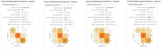
Figure A1.
Remaining Four Trials for “Training on All Six Data Points”.
Figure A1.
Remaining Four Trials for “Training on All Six Data Points”.
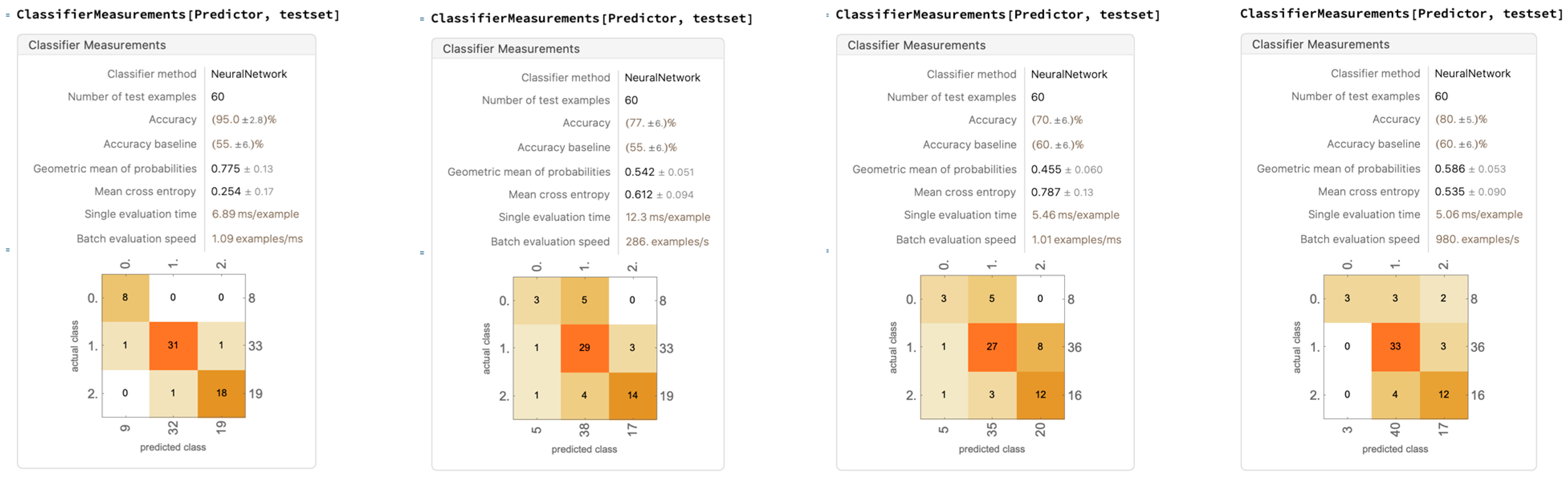
Appendix B
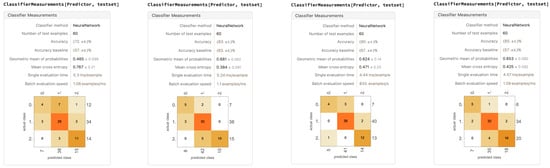
Figure A2.
Remaining Four Trials for “Dropping Out Racket Head Position”.
Figure A2.
Remaining Four Trials for “Dropping Out Racket Head Position”.
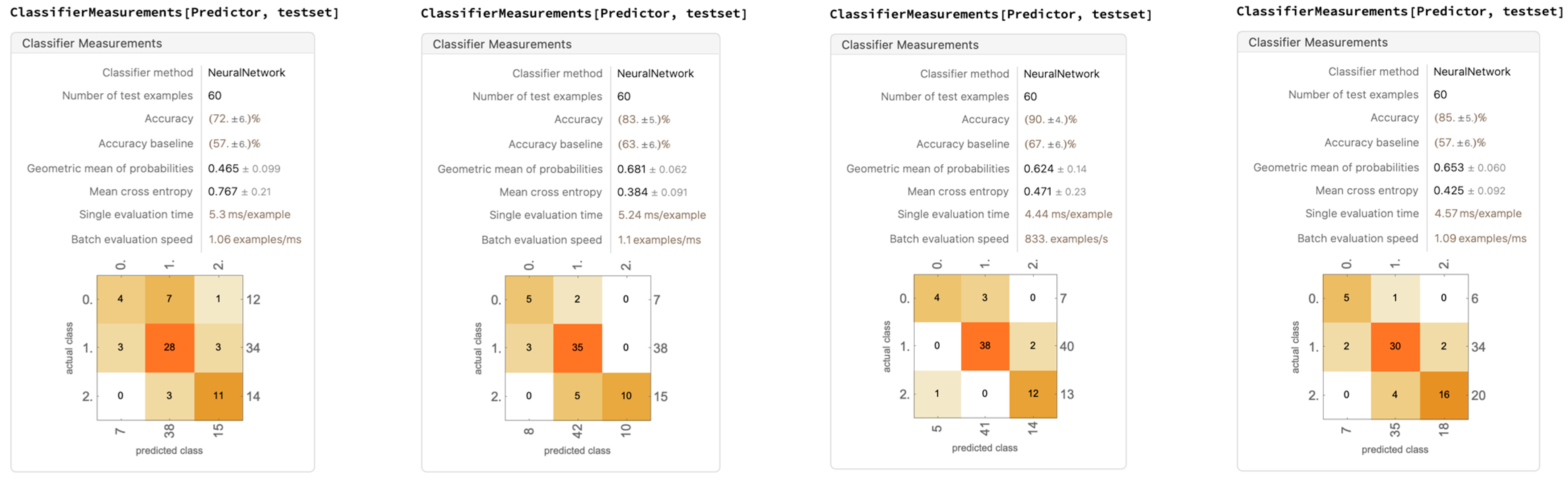
Appendix C
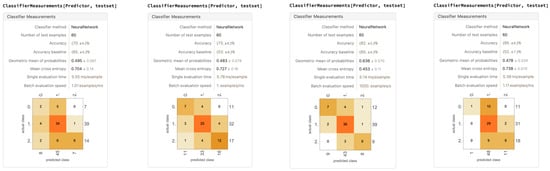
Figure A3.
Remaining Four Trials for “Dropping Out Racket Head Position and the First Bounce Position”.
Figure A3.
Remaining Four Trials for “Dropping Out Racket Head Position and the First Bounce Position”.

Appendix D
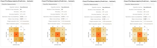
Figure A4.
Remaining Four Trials for “Dropping Out Racket Head Position and Second Bounce Position”.
Figure A4.
Remaining Four Trials for “Dropping Out Racket Head Position and Second Bounce Position”.
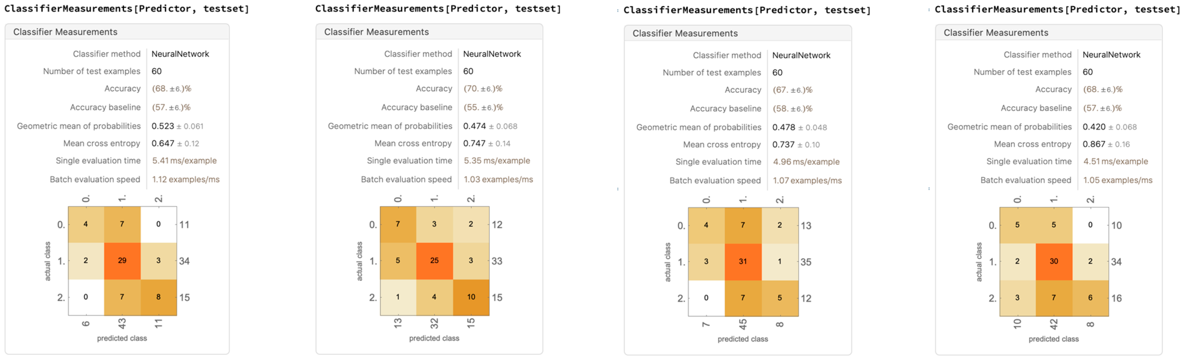
Appendix E
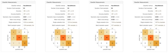
Figure A5.
Remaining Four Trials for “All Nine Modified Data (MD) Points”.
Figure A5.
Remaining Four Trials for “All Nine Modified Data (MD) Points”.
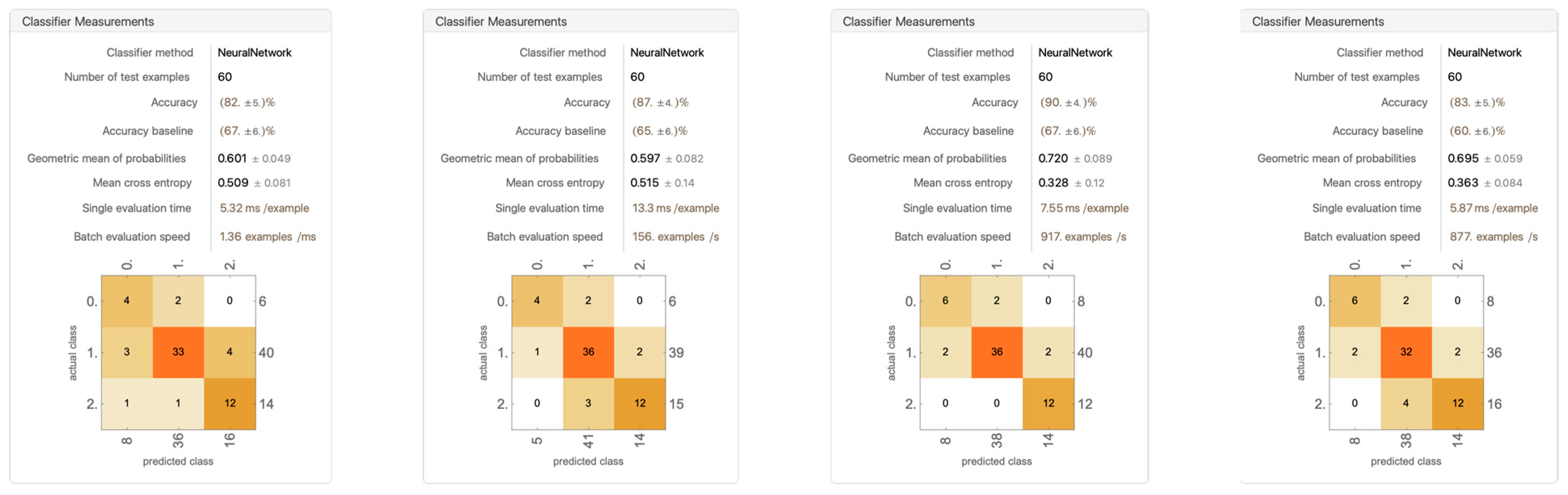
Appendix F
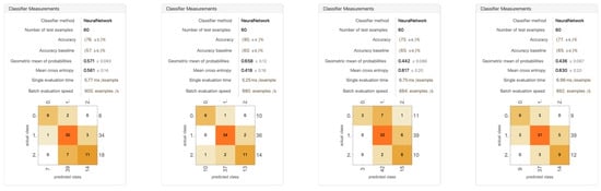
Figure A6.
Remaining Four Trials for “Including MD #1, #2, #3, #4, #6, #8, #9”.
Figure A6.
Remaining Four Trials for “Including MD #1, #2, #3, #4, #6, #8, #9”.
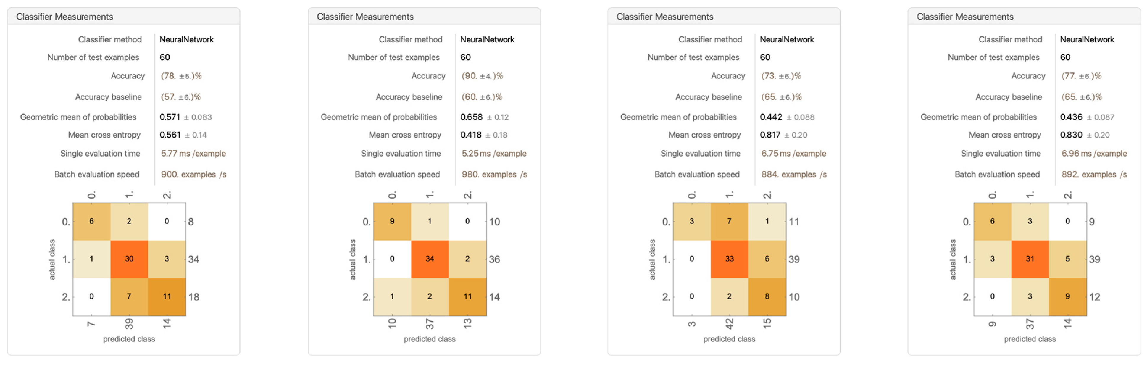
Appendix G
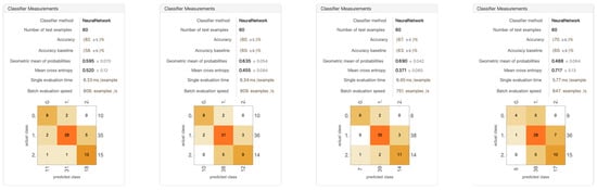
Figure A7.
Remaining Four Trials for “Including MD #1, #2, #3, #4, #6”.
Figure A7.
Remaining Four Trials for “Including MD #1, #2, #3, #4, #6”.
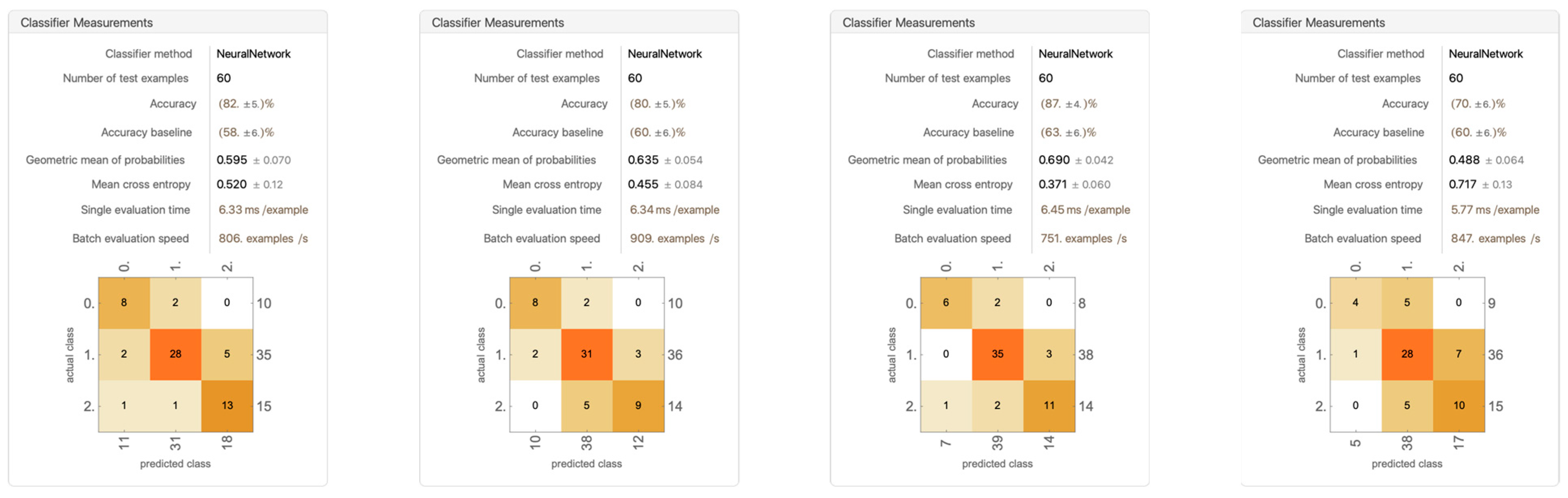
Appendix H
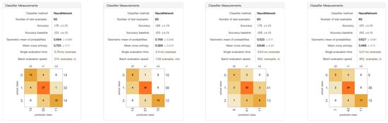
Figure A8.
Remaining Four Trials for “Training with all 21 Data Points”.
Figure A8.
Remaining Four Trials for “Training with all 21 Data Points”.
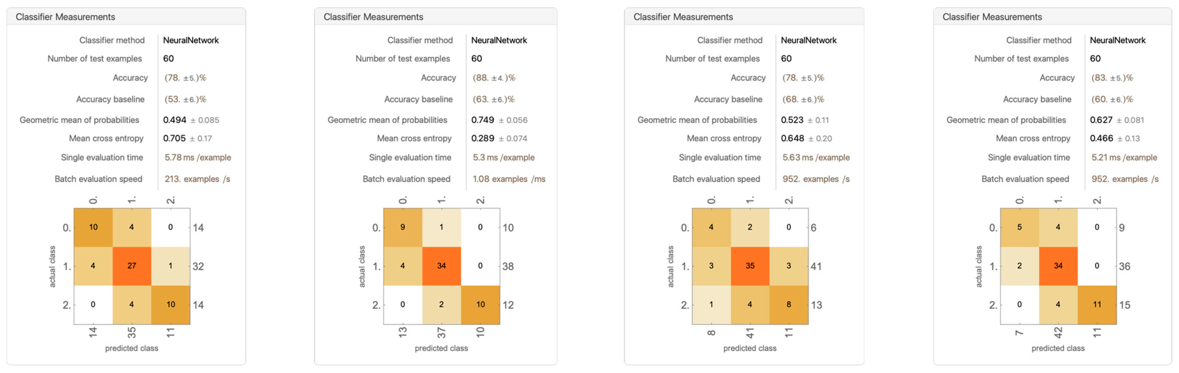
Appendix I
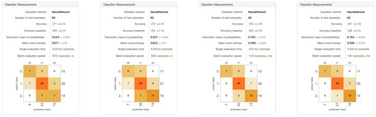
Figure A9.
Remaining Four Trials for “Training with PD 1–10 and All MD”.
Figure A9.
Remaining Four Trials for “Training with PD 1–10 and All MD”.
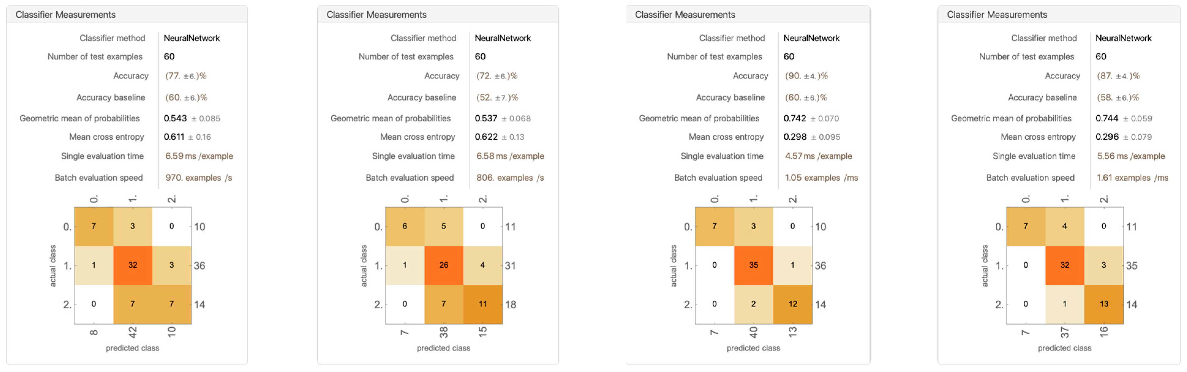
Appendix J

Figure A10.
Remaining Four Trials for “Training with PD 1–10 and MD #3, 5, 6, 8, and 9”.
Figure A10.
Remaining Four Trials for “Training with PD 1–10 and MD #3, 5, 6, 8, and 9”.
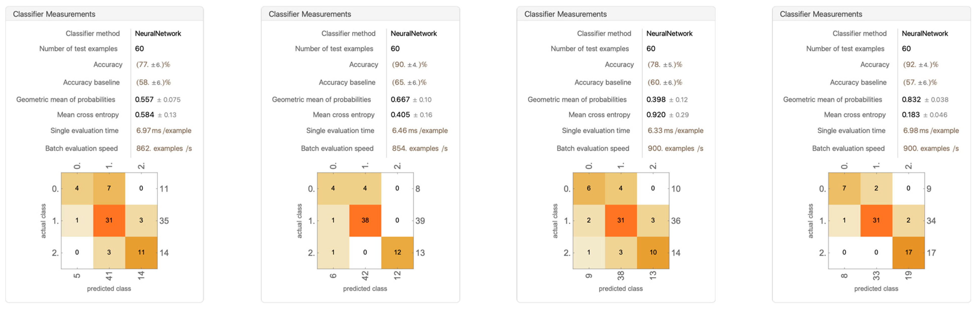
Appendix K. Glossary of Terms
- Accuracy: In machine learning, the degree to which the predictions of a model match the actual outcomes. High accuracy indicates effective performance of the model.
- Attacking Player (AP): In squash, the player who is actively making a play or shot at the ball.
- Back Wall: The wall at the rear of a squash court, often including a back glass wall for viewing.
- Ball’s Position in the Frame: A term used in video analysis of squash, referring to the location of the ball at a specific moment in time, usually captured in a video frame.
- Ball’s Projected First Bounce: The anticipated location where the ball will first bounce after being struck by a player.
- Ball’s Projected Second Bounce: The predicted location of the ball’s second bounce, important in determining the playability of a shot in squash.
- Clear the Ball: A term used in squash referring to the action of a player moving away from the ball after playing a shot, to avoid obstructing the opponent.
- Crowd Noise Influence: The effect that audience reactions can have on the performance or decisions of players and referees in sports, including squash.
- Data Augmentation: A technique in machine learning to increase the diversity of data available for training models, potentially applicable for enhancing squash match analysis.
- Dataset: A collection of data used for training machine learning models. In this context, it refers to the data gathered from squash matches for analysis.
- Distance Values: Metrics used in the analysis of squash matches, measuring distances between players, between players and the ball, and other spatial relationships relevant to decision making in the game.
- Fishing: In squash, “fishing” refers to a player’s tactic where they deliberately seek to draw a foul or earn a favorable decision from the referee rather than actively attempting to play the ball.
- Four-Wall Court: Describes the squash playing area, which is enclosed by four walls—front, back, and two sides.
- Front Wall: The main wall in a squash court where the ball must hit for a shot to be valid.
- Heatmaps: Visual representations showing the frequency or intensity of various phenomena in data analysis. In squash, heatmaps can indicate players’ positions or movements on the court over time.
- Interference: A situation in squash where one player’s play is obstructed by the presence or movement of the opponent.
- In-Bound Shot: A shot in squash that meets the game’s rules for a valid play, typically involving hitting the front wall above the tin and below the out line.
- Junior and College Squash: Levels of squash play that typically involve younger or student athletes, often with different dynamics and challenges compared to professional levels.
- Machine Learning (ML): A field of artificial intelligence that uses algorithms to analyze data, learn from its patterns, and make predictions or decisions without being explicitly programmed for specific tasks.
- Neural Networks: A subset of machine learning models designed to simulate the way human brains analyze and process information, consisting of interconnected nodes (neurons) working in layers to perform complex computations.
- Nick: The junction between the wall and the floor in a squash court; shots hitting the nick are often difficult to return.
- No Let: A decision in squash where the referee denies a player’s request to replay a point, often due to minimal or no interference, or if the player could not have played the ball regardless of the interference.
- Outline: The upper boundary on the front wall and side walls in squash; balls hitting above this line are out of play.
- Player Detection and Motion Analysis: Techniques in video analysis used to identify players’ positions and analyze their movements during a match.
- Positional Values: Data points referring to the positions of players, the ball, and other relevant spatial elements in a squash match.
- Professional and Amateur Squash Matches: Different levels of squash play, each with varying degrees of skill, rules, and formalities.
- Professional Squash Association (PSA): The global governing body for professional squash, responsible for organizing tournaments and maintaining rules and standards.
- Python: A high-level programming language known for its readability and versatility, widely used in data science, machine learning, and many other areas.
- Racket Head Position: The location of the head of the squash racket, significant in determining a player’s ability to hit the ball or the type of shot they are attempting.
- Rally: A series of back-and-forth shots between players in a squash game, beginning with a serve and continuing until a point is scored or a fault occurs.
- Referee Decision: In the context of squash, decisions made by a referee regarding points, fouls, or other aspects of the game, often influenced by player interactions and ball dynamics.
- Refereeing Standards: The guidelines and principles that referees use to make decisions in squash matches.
- Retreating Player (RP): The player who has just played the ball and is moving away to allow the opponent (attacking player) to play the next shot.
- Serve (and Return of Serve): The act of putting the ball into play at the beginning of a rally in squash. The return of serve is the opponent’s first shot in response to the serve.
- Shot Types: Various types of shots in squash like drives, volleys, boasts, drops, lobs, etc., each with specific strategic purposes.
- Side Wall: The walls on either side of a squash court, which can be used to alter the ball’s trajectory.
- Squash: A high-intensity racket sport played by two players in a four-walled court, where players hit a small rubber ball against the front wall under specific rules.
- Squash Court Dimensions: Standard measurements of a squash court, significant for understanding player movements and spatial strategies.
- Strategic Shots: Shots in squash that are executed with specific tactical intentions to gain an advantage over the opponent.
- Stroke: A refereeing decision in squash where one player is awarded a point due to significant interference by the opponent.
- TensorFlow: An open-source software library used for numerical computation and machine learning applications, particularly for training and deploying neural networks.
- Tin: The lower part of the front wall in a squash court, hitting which results in a fault or ‘out’ shot.
- Video Footage Reviewing and Labeling: The process of analyzing video recordings of squash matches to identify and label specific actions and decisions for data collection.
- Video Review System: A technology used in sports, including squash, for reviewing decisions or actions during a match, often involving slow-motion and multiple-angle replays.
- Wolfram Mathematica: A computational software used in scientific, engineering, and mathematical fields, known for its advanced data analysis capabilities.
- Yes Let: A call by the squash referee to replay a point, typically made when interference occurs, but it is deemed accidental or minimal.
References
- PSA World Tour. Squash Rules—The Basics Explained. PSA World Tour. 26 January 2023. Available online: https://www.psaworldtour.com/news/squash-rules-the-basics-explained/ (accessed on 20 August 2023).
- SQUASHTV. Elias v Asal|World Tour Finals 2022–2023|FREE LIVE MATCH! [Video]. YouTube. 21 June 2023. Available online: https://www.youtube.com/watch?v=Fg_7zxHsFUU&t=2123s (accessed on 20 August 2023).
- Brumann, C.; Kukuk, M.; Reinsberger, C. Evaluation of open-source and pre-trained deep convolutional neural networks suitable for player detection and motion analysis in squash. Sensors 2021, 21, 4550. [Google Scholar] [CrossRef]
- Hu, T.; Zheng, M.; Li, J.; Zhu, L.; Hu, J. A scene-adaptive motion detection model based on machine learning and data clustering. Multimed. Tools Appl. 2015, 74, 2821–2839. [Google Scholar] [CrossRef]
- Menashe, J.; Kelle, J.; Genter, K.; Hanna, J.; Liebman, E.; Narvekar, S.; Zhang, R.; Stone, P. Fast and Precise Black and White Ball Detection for RoboCup Soccer. In RoboCup 2017: Robot World Cup XXI; Akiyama, H., Obst, O., Sammut, C., Tonidandel, F., Eds.; RoboCup 2017. Lecture Notes in Computer Science; Springer: Cham, Switzerland, 2018; Volume 11175. [Google Scholar]
- Hiemann, A.; Kautz, T.; Zottmann, T.; Hlawitschka, M. Enhancement of Speed and Accuracy Trade-Off for Sports Ball Detection in Videos—Finding Fast Moving, Small Objects in Real Time. Sensors 2021, 21, 3214. [Google Scholar] [CrossRef]
- Bayram, F.; Garbarino, D.; Barla, A. Predicting Tennis Match Outcomes with Network Analysis and Machine Learning. In SOFSEM 2021: Theory and Practice of Computer Science. SOFSEM 2021, Bolzano-Bozen, Italy, 25–29 January 2021; Bureš, T., Ed.; Lecture Notes in Computer Science; Springer: Cham, Switzerland, 2021; Volume 12607. [Google Scholar]
- Maier, T.; Meister, D.; Trösch, S.; Wehrlin, J.P. Predicting biathlon shooting performance using machine learning. J. Sports Sci. 2018, 36, 2333–2339. [Google Scholar] [CrossRef] [PubMed]
- Capobianco, G.; Di Giacomo, U.; Mercaldo, F.; Nardone, V.; Santone, A. Can Machine Learning Predict Soccer Match Results? In Proceedings of the 11th International Conference on Agents and Artificial Intelligence, Prague, Czech Republic, 19–21 February 2019; SciTePress: Setúbal, Portugal, 2019; Volume 2, pp. 458–465. [Google Scholar] [CrossRef]
- Nguyen, N.H.; Nguyen DT, A.; Ma, B.; Hu, J. The application of machine learning and deep learning in sport: Predicting NBA players’ performance and popularity. J. Inf. Telecommun. 2021, 6, 217–235. [Google Scholar] [CrossRef]
- Draschkowitz, L.; Draschkowitz, C.; Hlavacs, H. Predicting Shot Success for Table Tennis Using Video Analysis and Machine Learning. In Intelligent Technologies for Interactive Entertainment. INTETAIN 2014, Chicago, IL, USA, 9–11 July 2014; Reidsma, D., Choi, I., Bargar, R., Eds.; Lecture Notes of the Institute for Computer Sciences, Social Informatics and Telecommunications Engineering; Springer: Cham, Switzerland, 2014; Volume 136. [Google Scholar] [CrossRef]
- Balmer, N.J.; Nevill, A.M.; Lane, A.M.; Ward, P. Influence of crowd noise on soccer refereeing consistency in soccer. J. Sport Behav. 2007, 30, 130. [Google Scholar]
- Dohmen, T.; Sauermann, J. REFEREE BIAS. J. Econ. Surv. 2016, 30, 679–695. [Google Scholar] [CrossRef]
- Morgulev, E.; Azar, O.H.; Lidor, R.; Sabag, E.; Bar-Eli, M. Searching for Judgment Biases Among Elite Basketball Referees. Front. Psychol. 2018, 9, 2637. [Google Scholar] [CrossRef] [PubMed]
- Murray, S.; James, N.; Perš, J.; Mandeljc, R.; Vučković, G. Using a situation awareness approach to determine decision-making behaviour in squash. J. Sports Sci. 2018, 36, 1415–1422. [Google Scholar] [CrossRef] [PubMed]
- Professional Squash Association (PSA). PSA Squash TV [YouTube Channel]. YouTube. 9 January 2012. Available online: https://www.youtube.com/@squashtv (accessed on 20 August 2023).
- SQUASHTV. Squash: Full Match—2014 El Gouna International SF—Elshorbagy v Gaultier [Video]. YouTube. 25 December 2014. Available online: https://www.youtube.com/watch?v=HyX7IV-YhKo&list=PlxmhcE3iz1lCnuIXg2hOHD29HooENItXg&index=130 (accessed on 20 August 2023).
- PSA World Tour. PSA to Roll Out Video Review for All TV Events. World Squash. 8 September 2011. Available online: https://www.worldsquash.org/psa-to-roll-out-video-review-for-all-tv-events/ (accessed on 20 August 2023).
- Chang, Y.H.; Chung, C.Y. Classification of Breast Cancer Malignancy Using Machine Learning Mechanisms in TensorFlow and Keras. In Future Trends in Biomedical and Health Informatics and Cybersecurity in Medical Devices. ICBHI 2019. IFMBE Proceedings, Taipei, Taiwan, 17–20 April 2019; Lin, K.P., Magjarevic, R., de Carvalho, P., Eds.; Springer: Cham, Switzerland, 2020; Volume 74. [Google Scholar]
- Kompella, S.; Likith Vishal, B.; Sivalaya, G. A Comparative Study of Classification Algorithms Over Images Using Machine Learning and TensorFlow. In Mobile Computing and Sustainable Informatics. Lecture Notes on Data Engineering and Communications Technologies; Shakya, S., Bestak, R., Palanisamy, R., Kamel, K.A., Eds.; Springer: Singapore, 2022; Volume 68. [Google Scholar]
- Gundina, M.A.; Zhdanovich, M.N. Automatic localization of a car license plate in the Wolfram Mathematica system. Sci. Technol. 2022, 21, 367–373. [Google Scholar] [CrossRef]
- Ortigoza, G.; Zapata, U. COVID-19 Projections: A Simple Machine Learning Approach. In Proceedings of the 2021 IEEE International Conference on Engineering Veracruz (ICEV), Boca del Río, Veracruz, Mexico, 25–28 October 2021; pp. 1–4. [Google Scholar] [CrossRef]
- SQUASHTV. PSA Rewind: Willstrop v Gawad—2018 Grasshopper Cup—Full Squash Match [Video]. YouTube. 18 March 2020. Available online: https://www.youtube.com/watch?v=2T6AXYrhwZQ&list=PLxmhcE3iz1lCnuIXg2hOHD29HooENItXg&index=72 (accessed on 20 August 2023).
- SQUASHTV. Squash: Full Match—2014 Tournament of Champions—Shabana v Matthew [Video]. YouTube. 24 December 2014. Available online: https://www.youtube.com/watch?v=OI0xHMRut88&list=PLxmhcE3iz1lCnuIXg2hOHD29HooENItXg&index=125 (accessed on 20 August 2023).
- SQUASHTV. Squash: Full Match—2014 British Open SF—Matthew v Elshorbagy (British Open) [Video]. YouTube. 25 December 2014. Available online: https://www.youtube.com/watch?v=nwzMnIECgDk&list=PLxmhcE3iz1lCnuIXg2hOHD29HooENItXg&index=127 (accessed on 20 August 2023).
- SQUASHTV. Squash Archive: Shabana v Matthew—2012/13 World Tour Finals [Video]. YouTube. 5 June 2019. Available online: https://www.youtube.com/watch?v=AASrbKRyAUo&list=PLxmhcE3iz1lCnuIXg2hOHD29HooENItXg&index=79 (accessed on 20 August 2023).
- SQUASHTV. SQUASH: Full Match—2012 PSA World Championship Final—Ashour v Elshorbagy [Video]. YouTube. 24 December 2013. Available online: https://www.youtube.com/watch?v=s6QcWY5wEak&list=PLxmhcE3iz1lCnuIXg2hOHD29HooENItXg&index=119 (accessed on 20 August 2023).
- SQUASHTV. Squash: Full Match—Canary Wharf 2010 SF—Matthew v Willstrop [Video]. YouTube. 5 October 2013. Available online: https://www.youtube.com/watch?v=HtwckCfSIHU&list=PLxmhcE3iz1lCnuIXg2hOHD29HooENItXg&index=118 (accessed on 20 August 2023).
- SQUASHTV. Squash: Full Match—2011 World Series Finals, Final—Shabana v Gaultier [Video]. YouTube. 5 October 2013. Available online: https://www.youtube.com/watch?v=fdYZePDe69s&list=PLxmhcE3iz1lCnuIXg2hOHD29HooENItXg&index=118 (accessed on 20 August 2023).
- SQUASHTV. Squash: Free (Match) Friday—Ashour v Gaultier—British Open 2013 Final [Video]. YouTube. 18 March 2016. Available online: https://www.youtube.com/watch?v=5O3fpxcExu0&list=PLxmhcE3iz1lCnuIXg2hOHD29HooENItXg&index=115 (accessed on 20 August 2023).
- SQUASHTV. Squash: Farag v Coll—Full Match—British Open 2019—Christmas Cracker [Video]. YouTube. 25 December 2019. Available online: https://www.youtube.com/watch?v=ntNh7L1pTag&list=PLxmhcE3iz1lCnuIXg2hOHD29HooENItXg&index=77 (accessed on 20 August 2023).
- Saini, V. Average Shoulder Width for Men and Women. Fitness Volt. 18 April 2023. Available online: https://fitnessvolt.com/average-shoulder-width/#:~:text=According%20to%20the%20same%20CDC,the%2030%2D39%20age%20group (accessed on 20 August 2023).
- Wolfram. (n.d.). Classifying Data with Neural Networks. Classifying Data with Neural Networks-Wolfram Language Documentation. Available online: https://reference.wolfram.com/language/tutorial/NeuralNetworksClassification.html (accessed on 20 August 2023).
- Bordner, S.S. Why You Don’t Have to Choose between Accuracy and Human Officiating (But You Might Want to Anyway). Philosophies 2019, 4, 33. [Google Scholar] [CrossRef]
- Williams, M.T. MLB Umpires Missed 34,294 Ball-Strike Calls in 2018. Bring on Robo-Umps? Boston University, BU Today. 8 April 2019. Available online: https://www.bu.edu/today/2019/mlb-umpires-strike-zone-accuracy/ (accessed on 14 January 2024).
- Tranfield, J.K. Stress and Coping in High Performance Squash Coaching. Doctoral Dissertation, Loughborough University, Loughborough, UK, 2002; p. 527. Available online: https://repository.lboro.ac.uk/articles/Stress_and_coping_in_high_performance_squash_coaching_/9609314/files/17256035.pdf (accessed on 20 August 2023).
- Ma, Enqi. Personal Communication with Juan Jose Torres (unpublished), 2021 Squash US Junior Open U17 Champion, 2022 Squash US Junior Open U19 Champion, 2022 Squash World Junior Championship U19 #5, 14 Jan 2024.
- SQUASHTV. Squash: 100k Subscriber Special—Matthew v Gaultier ToC 2018 Full Match [Video]. YouTube. 18 December 2018. Available online: https://www.youtube.com/watch?v=6lniVi_ScJI&list=PLxmhcE3iz1lCnuIXg2hOHD29HooENItXg&index=82 (accessed on 20 August 2023).
- SQUASHTV. Best Squash Match Ever? 2014 World Championship Final: Ashour v Elshorbagy—Full Match [Video]. YouTube. 25 December 2014. Available online: https://www.youtube.com/watch?v=-xs8EUlCL5o&list=PLxmhcE3iz1lCnuIXg2hOHD29HooENItXg&index=116 (accessed on 20 August 2023).
- SQUASHTV. Squash: Free (Match) Friday—2013/14 World Series Finals—Elshorbagy v Ashour FINAL [Video]. YouTube. 6 May 2016. Available online: https://www.youtube.com/watch?v=lpEQp1raU00&list=PLxmhcE3iz1lCnuIXg2hOHD29HooENItXg&index=113 (accessed on 20 August 2023).
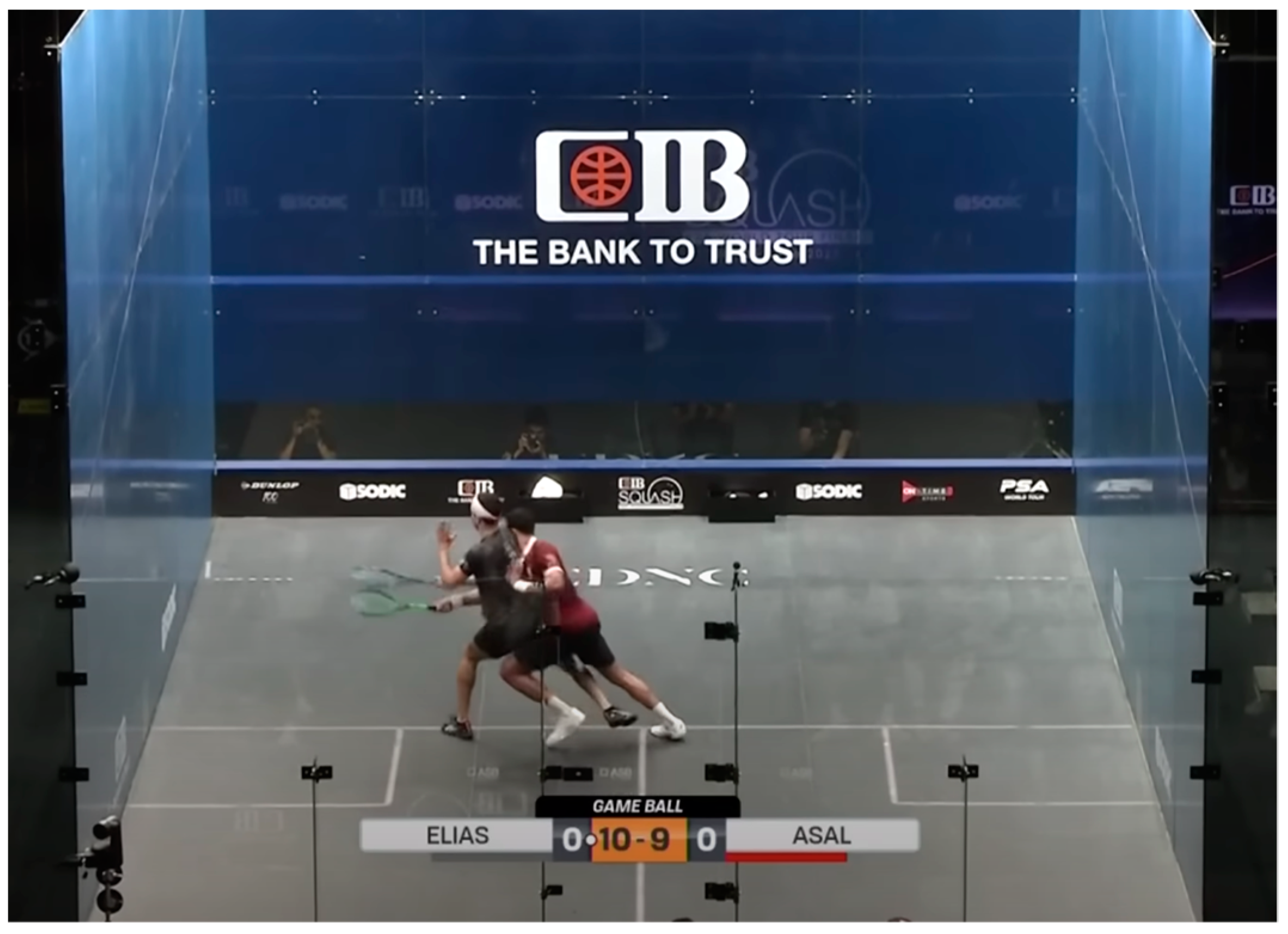
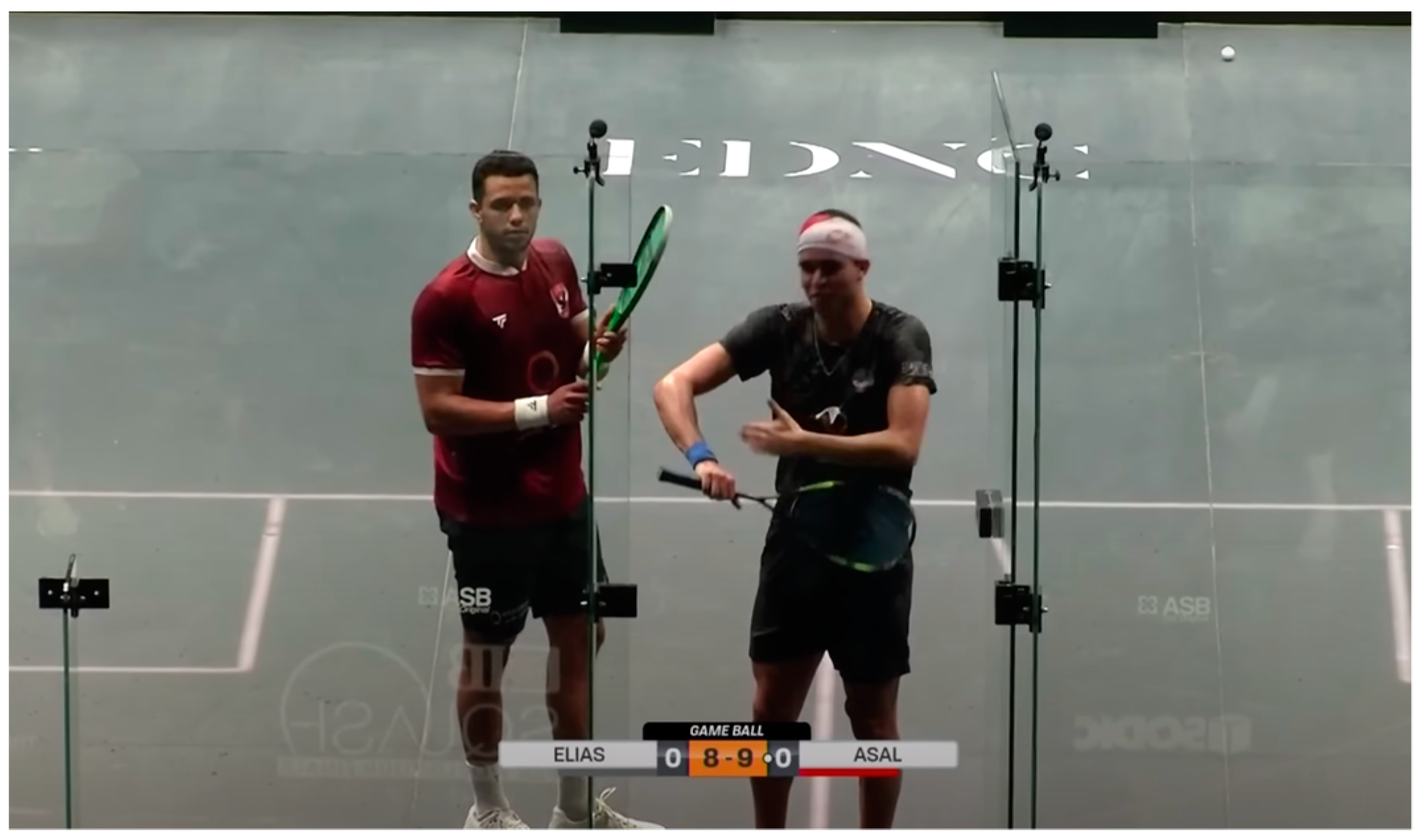
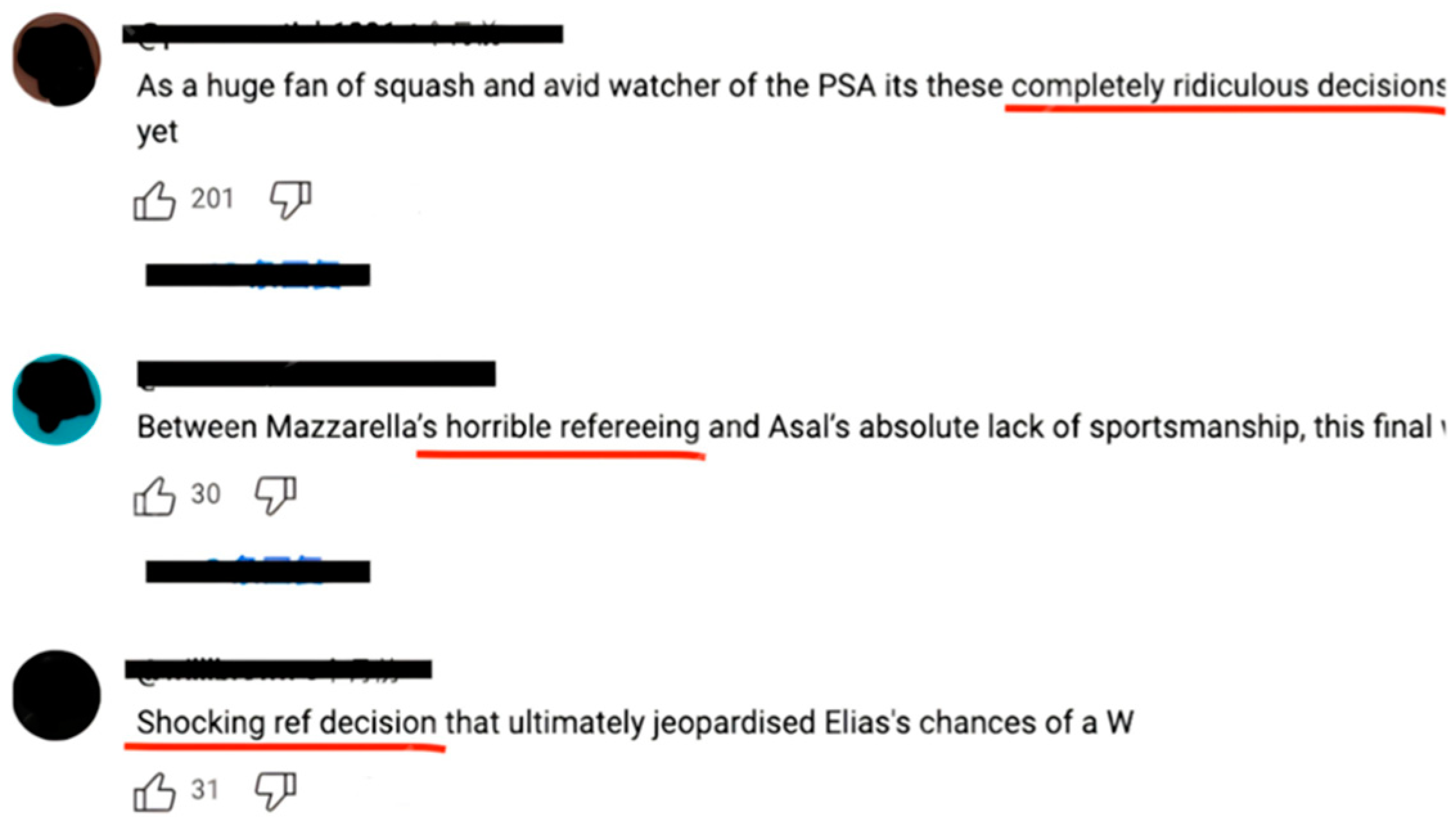
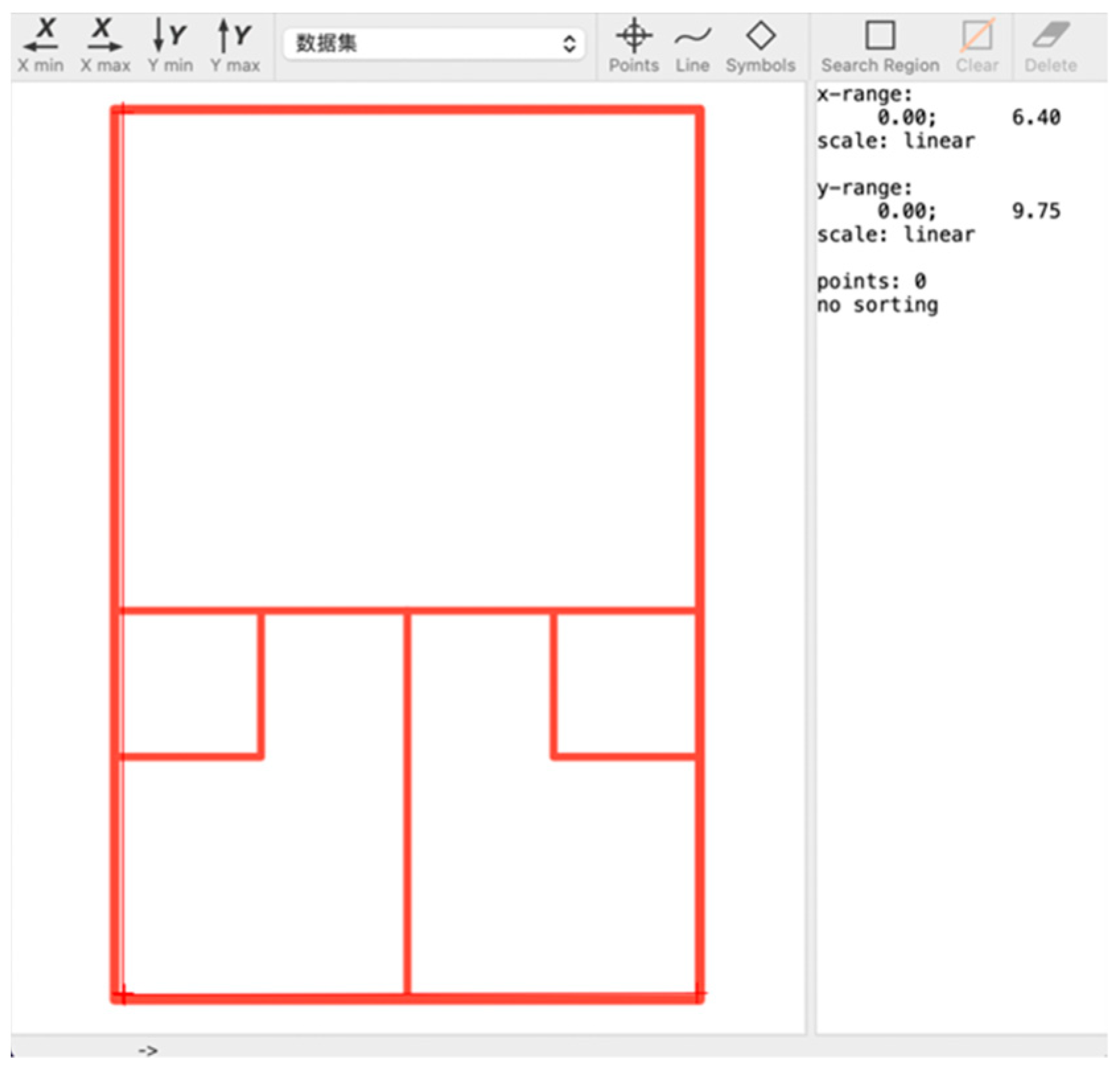


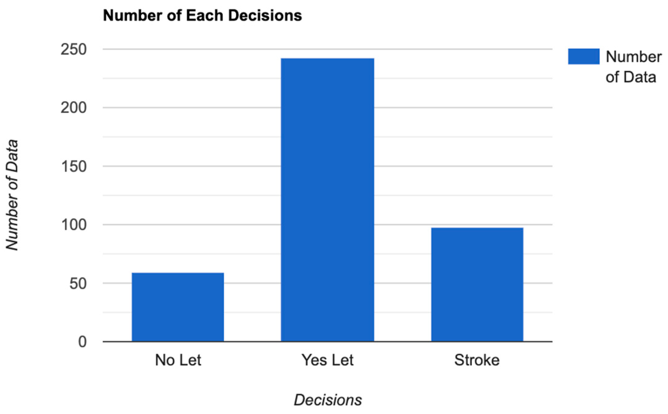

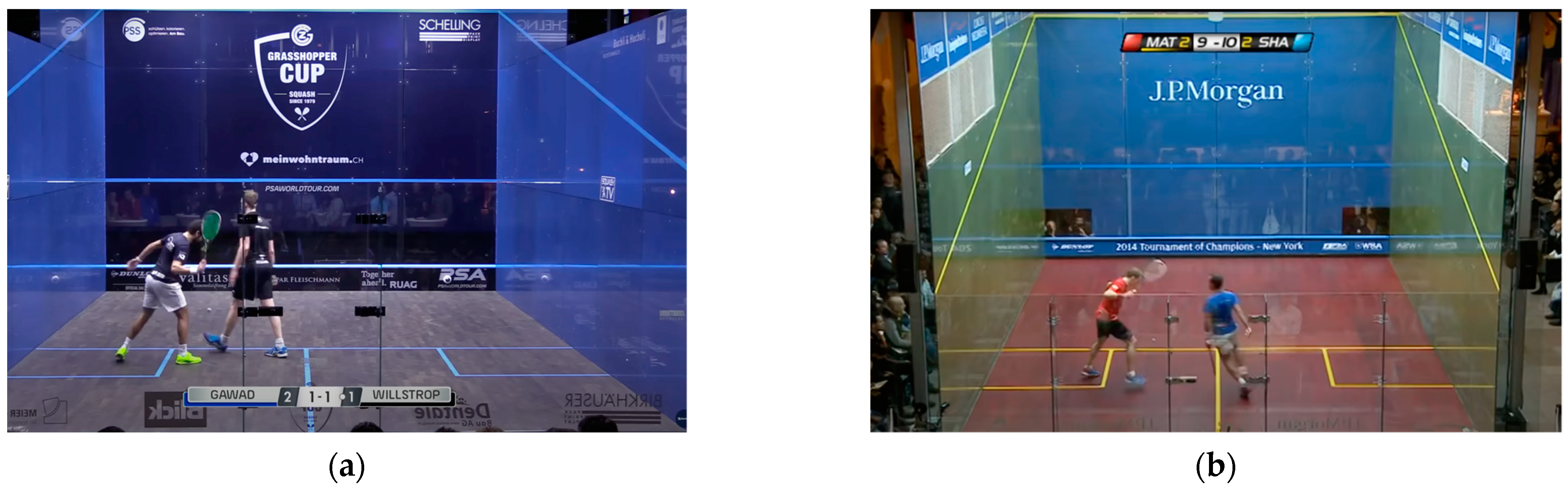


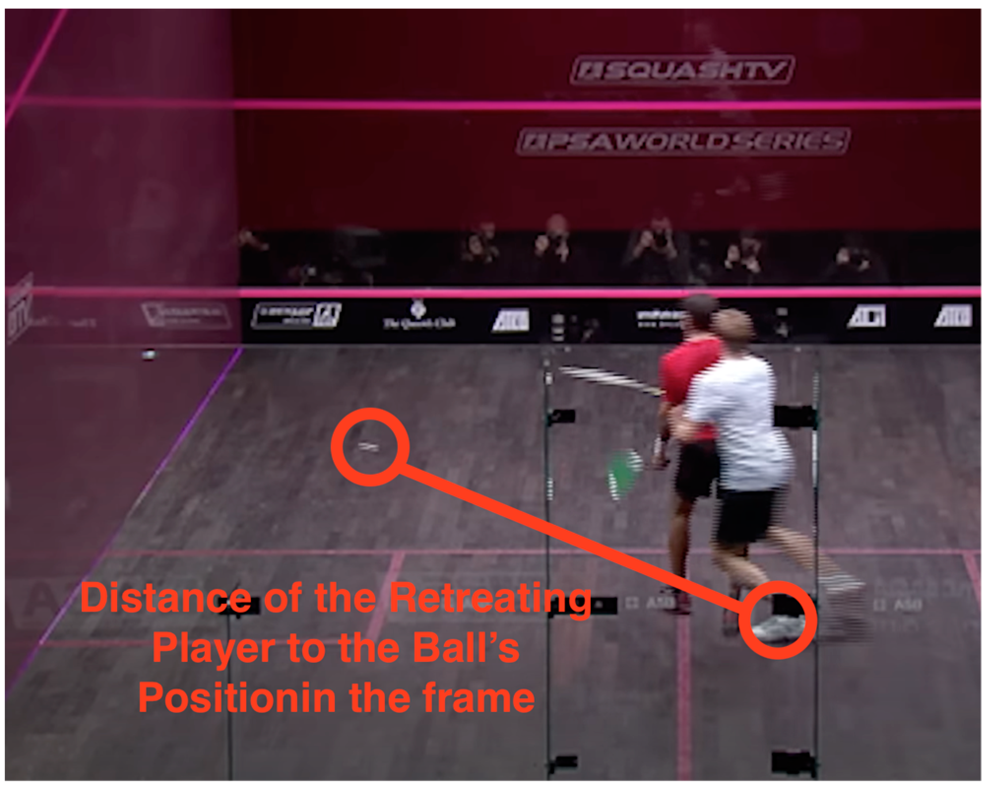

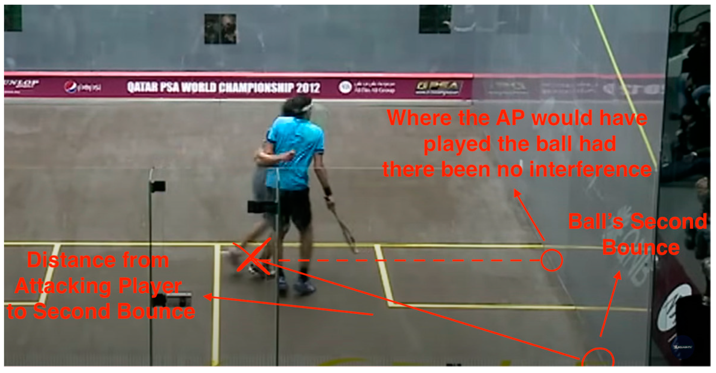

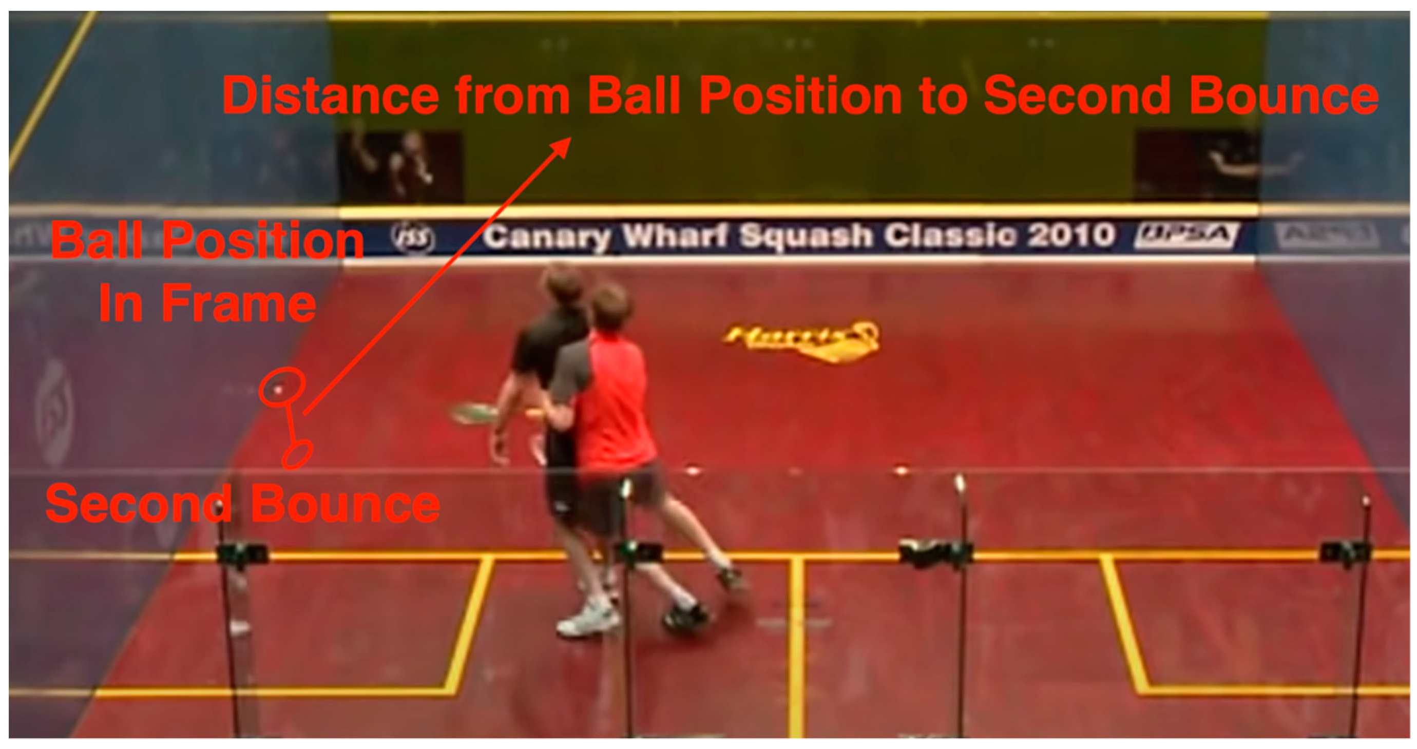
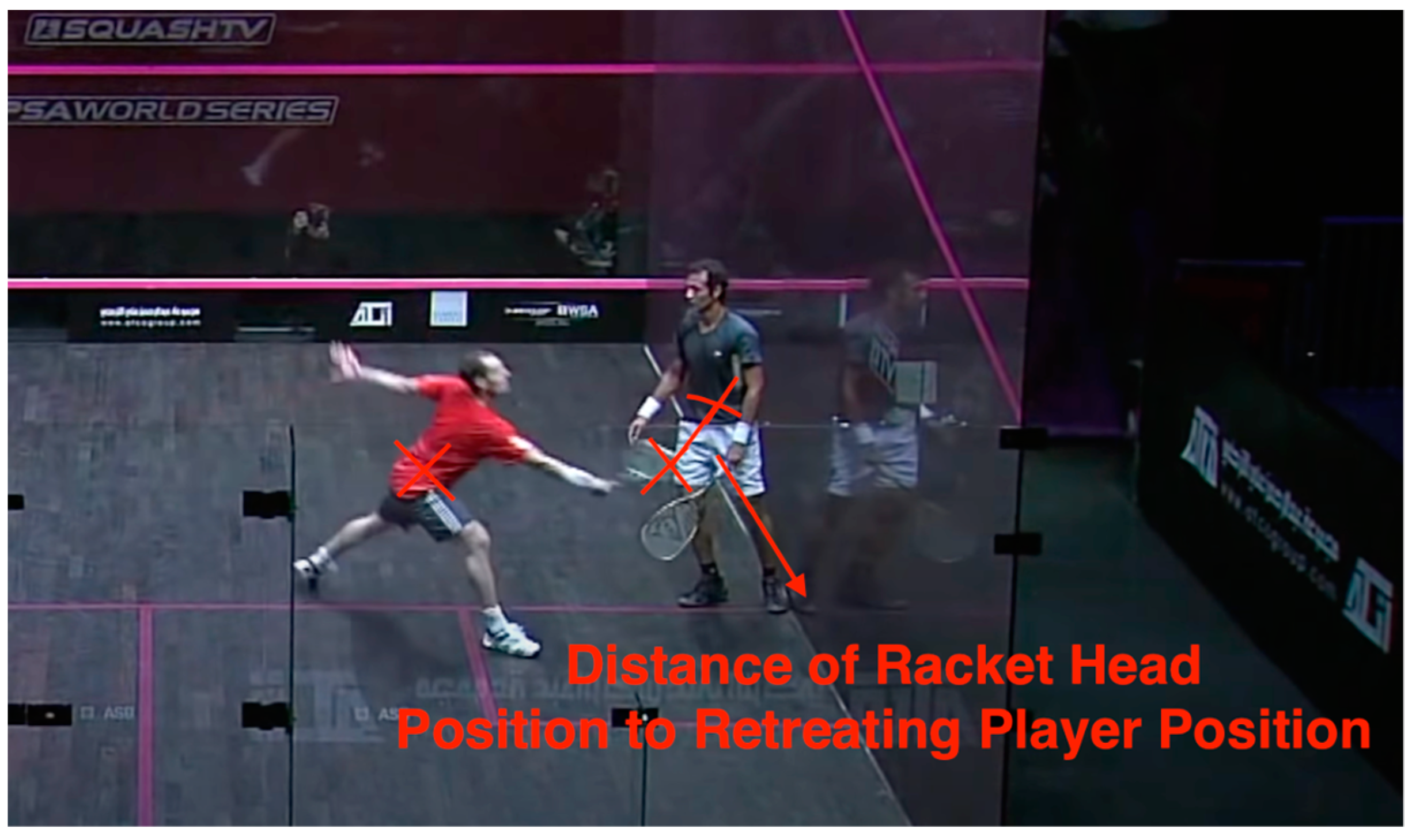

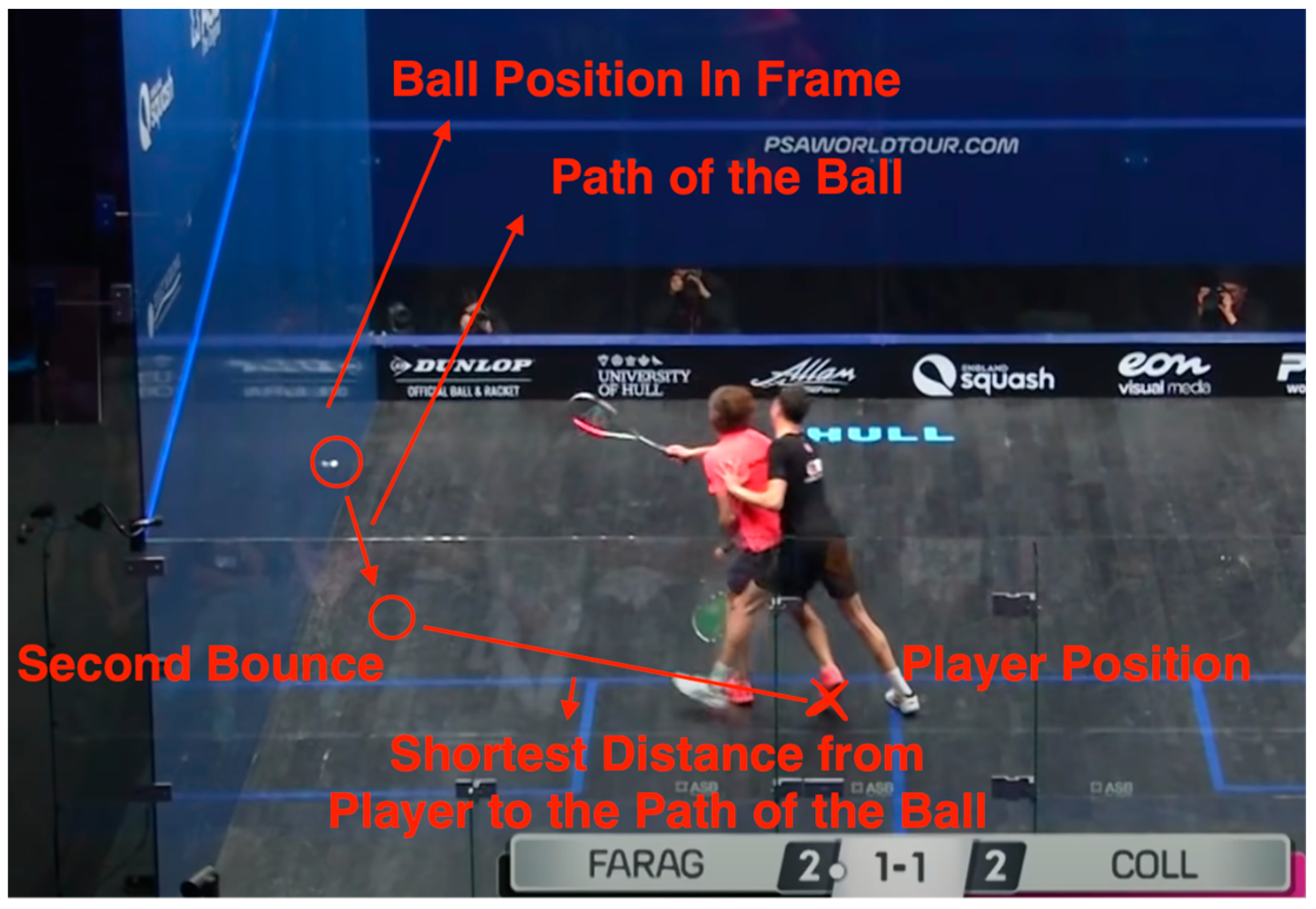
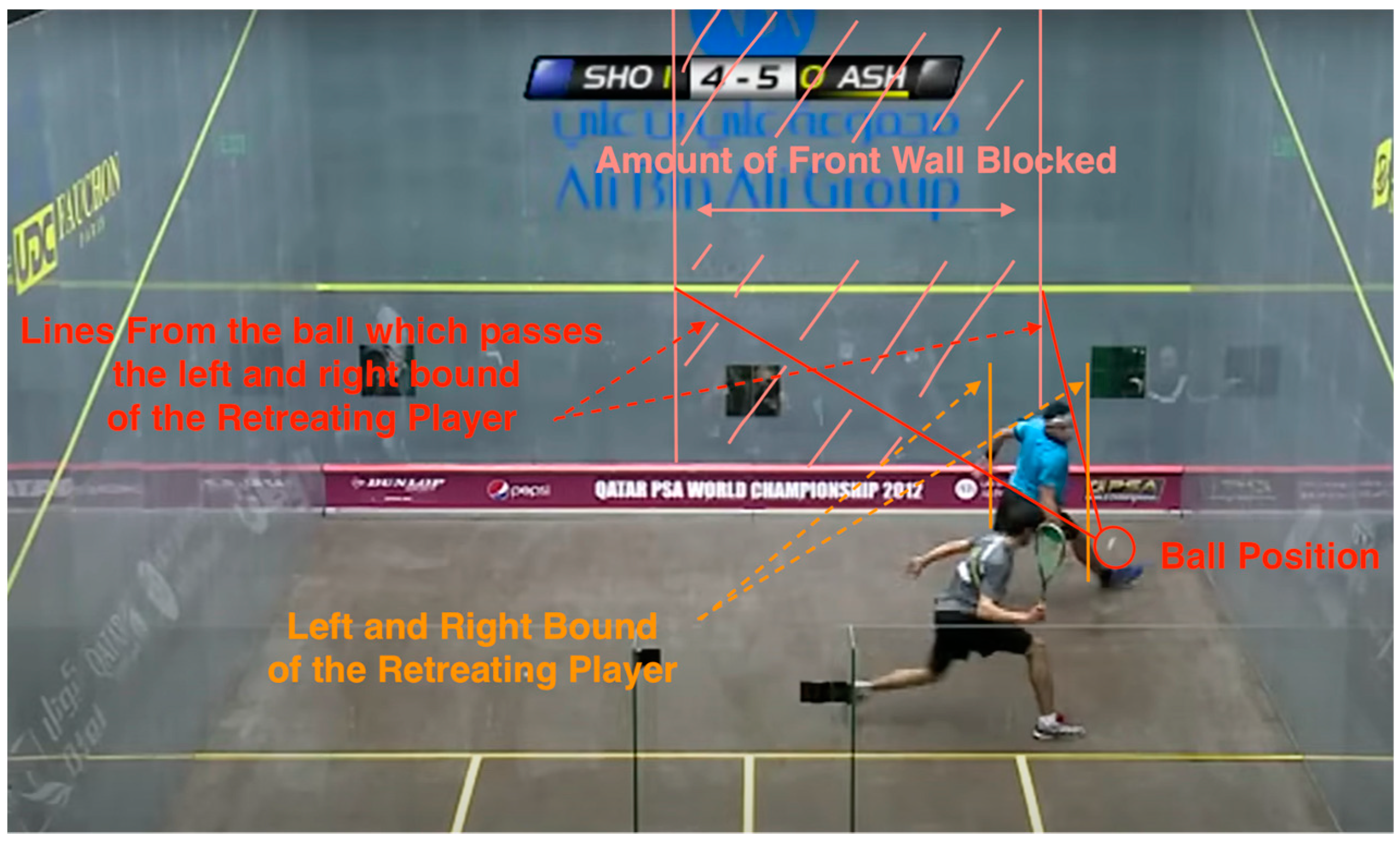

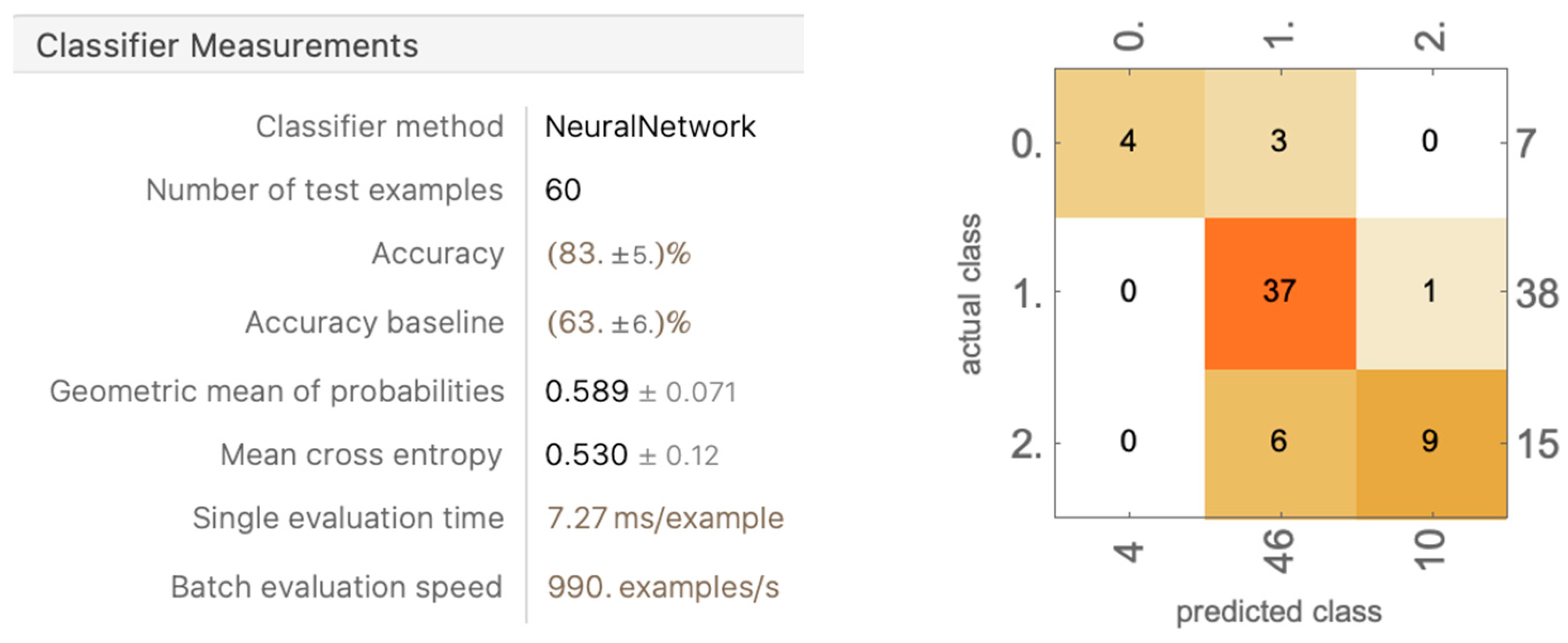
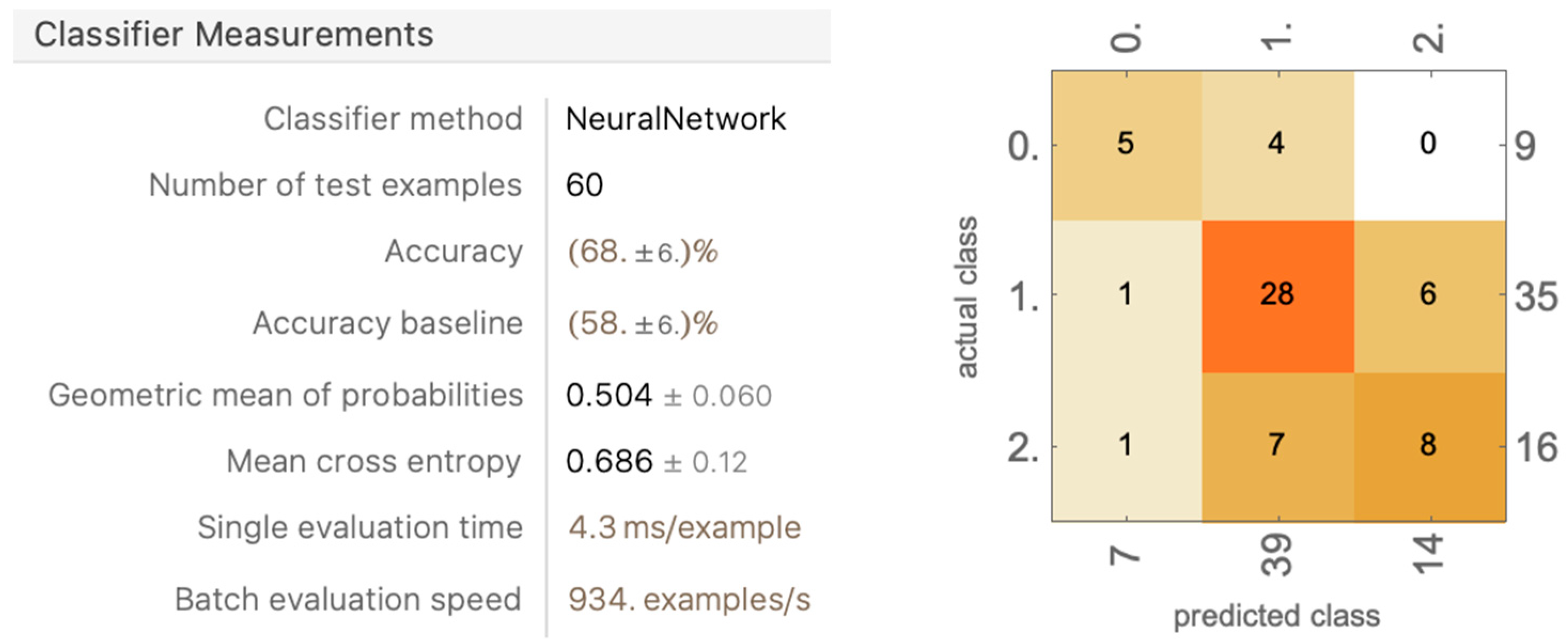
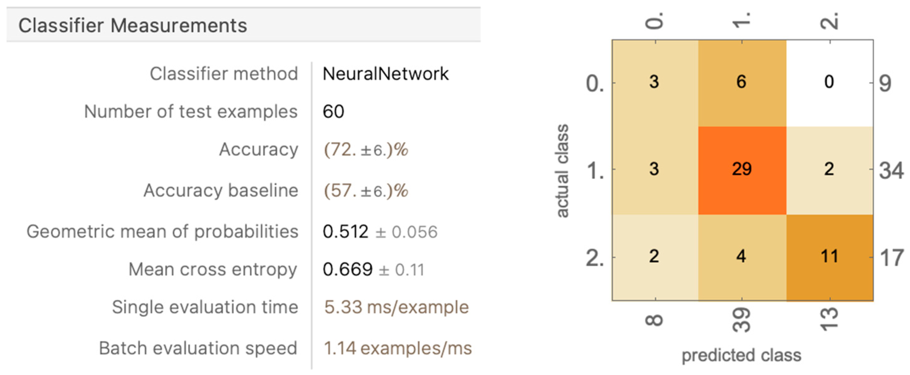
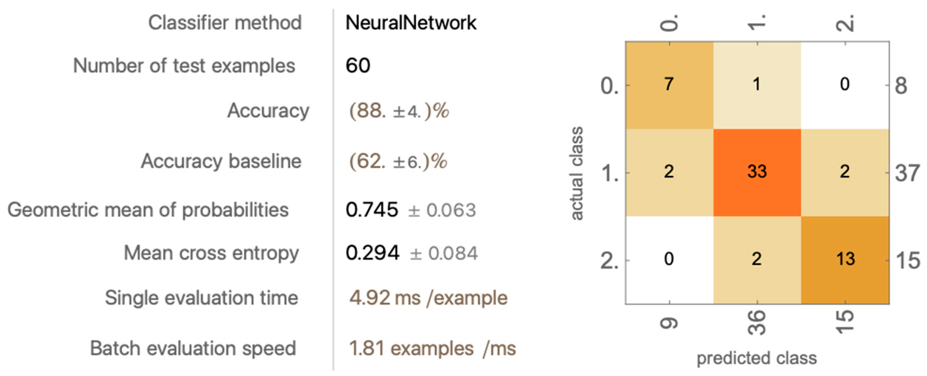
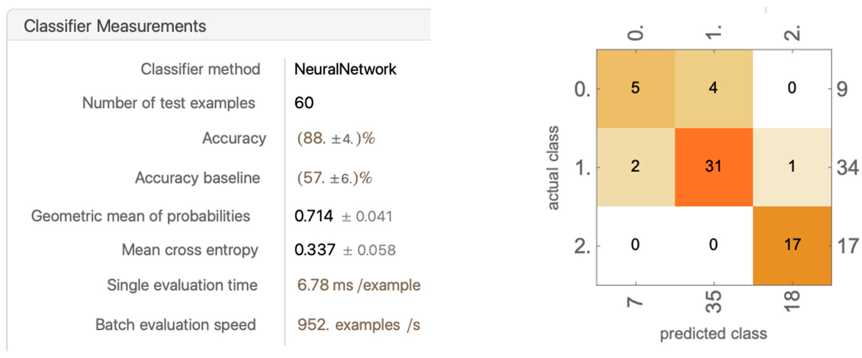

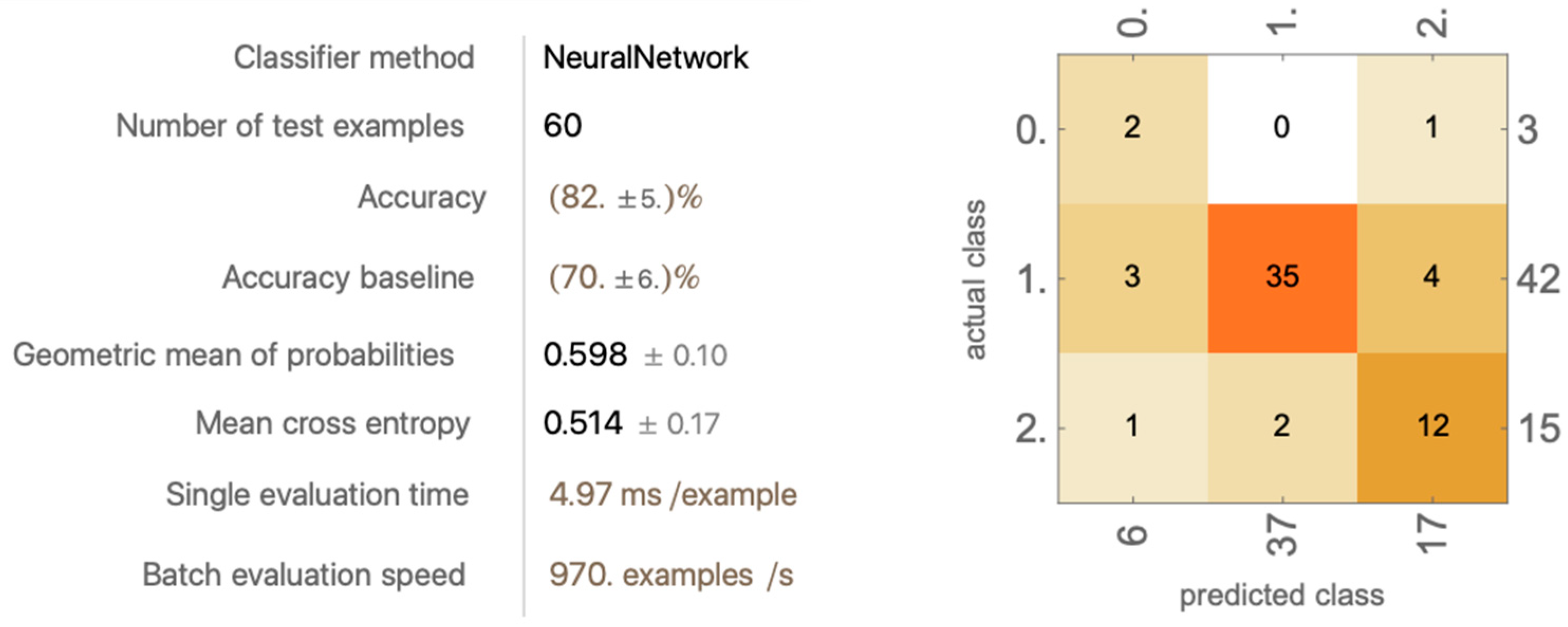
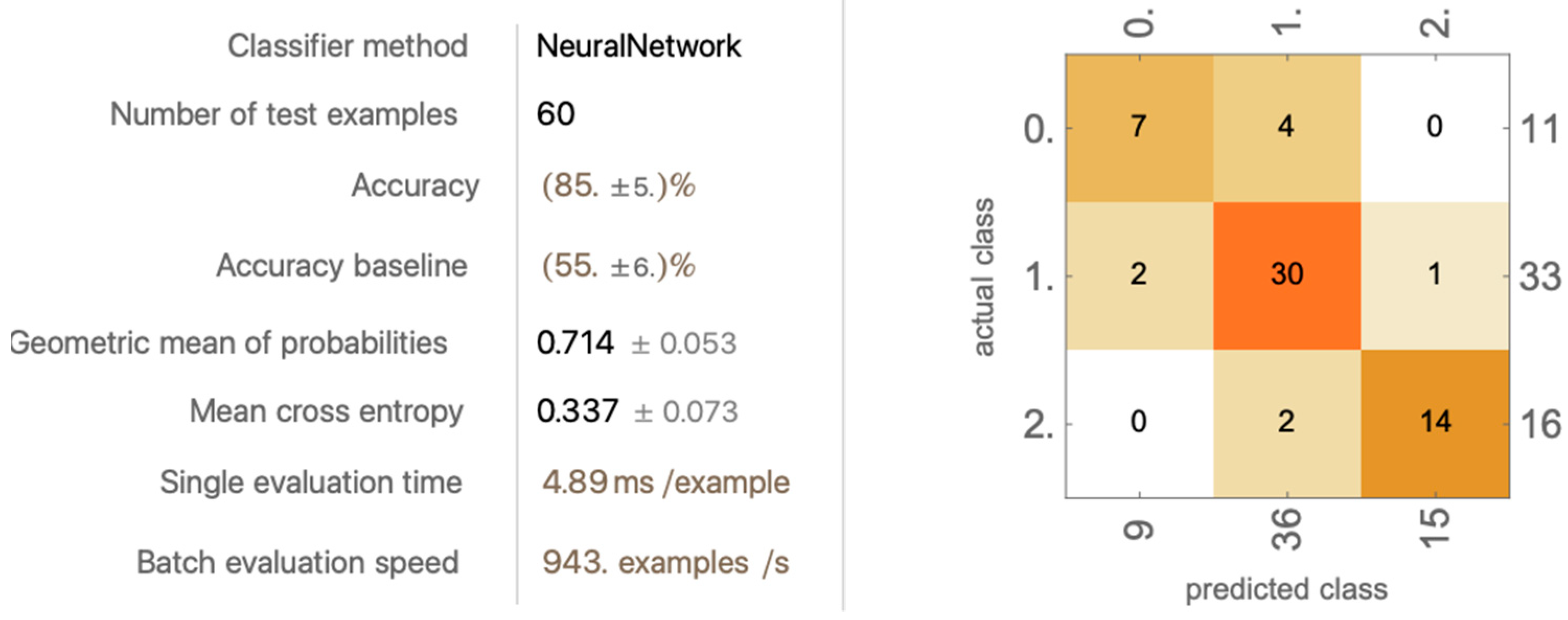

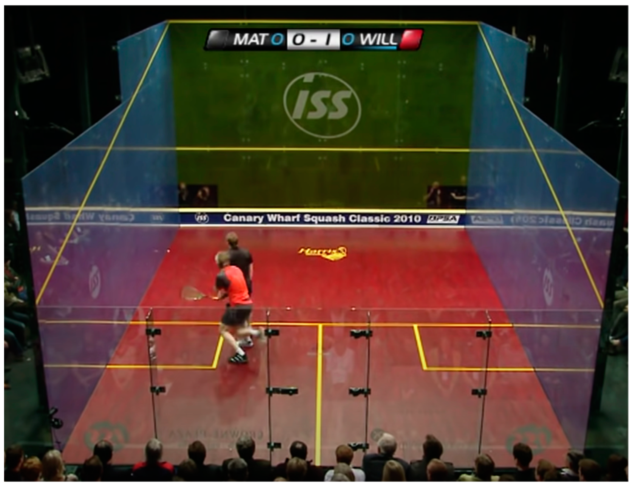

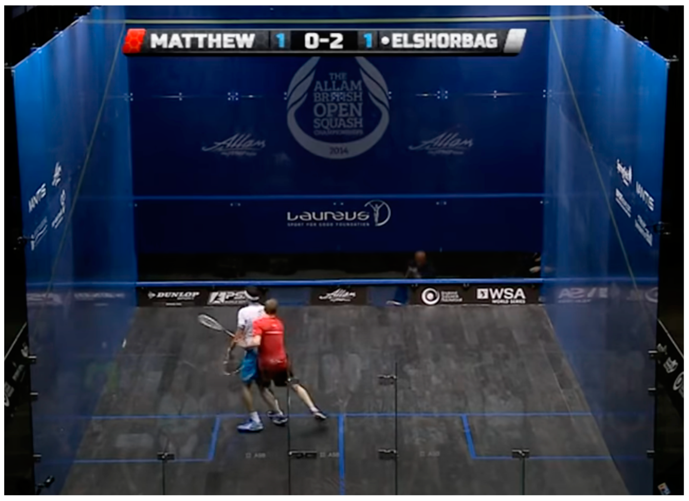
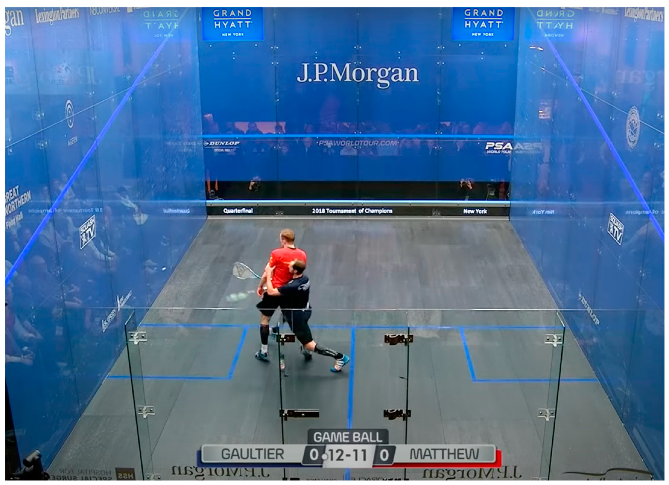
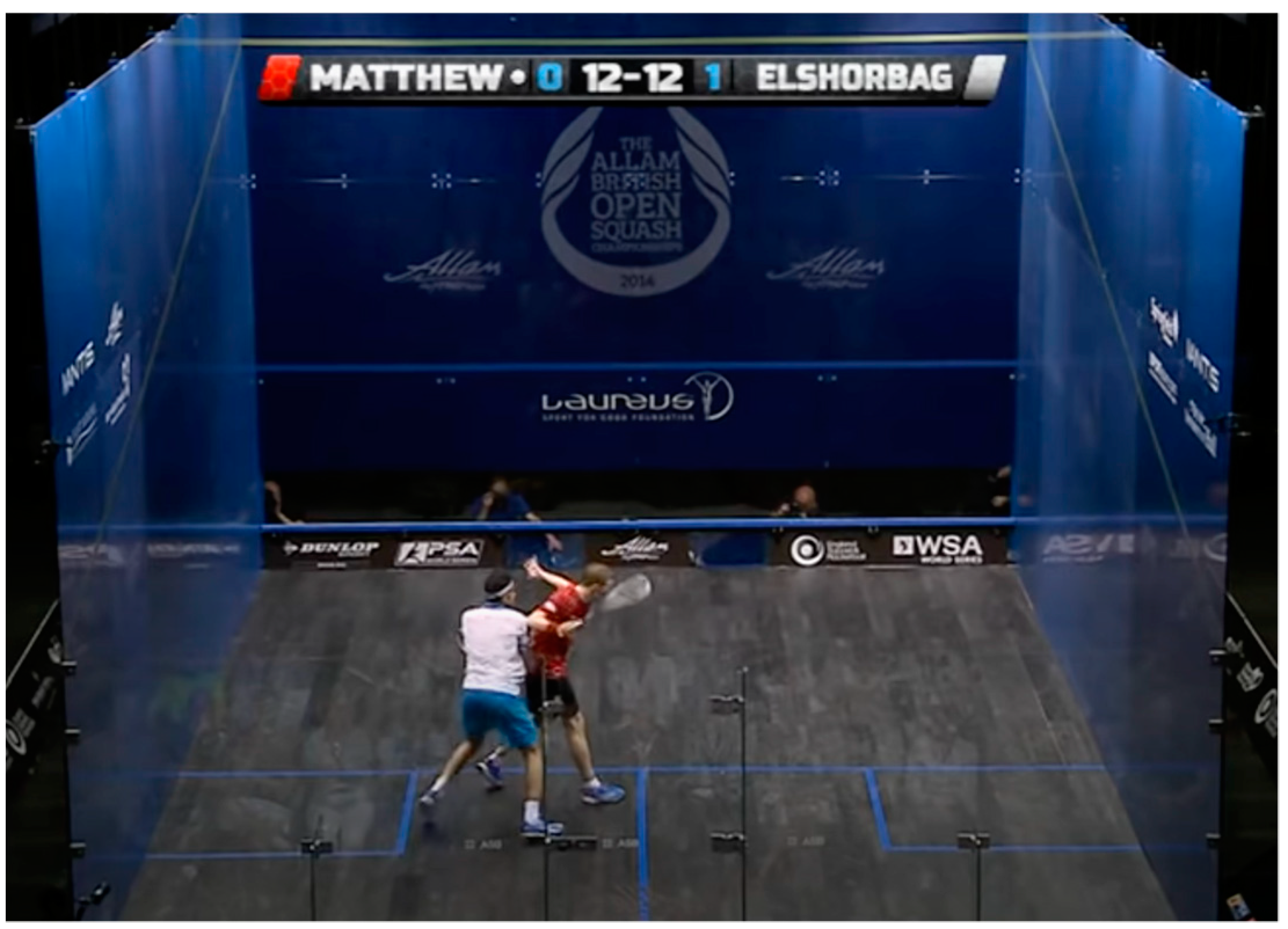

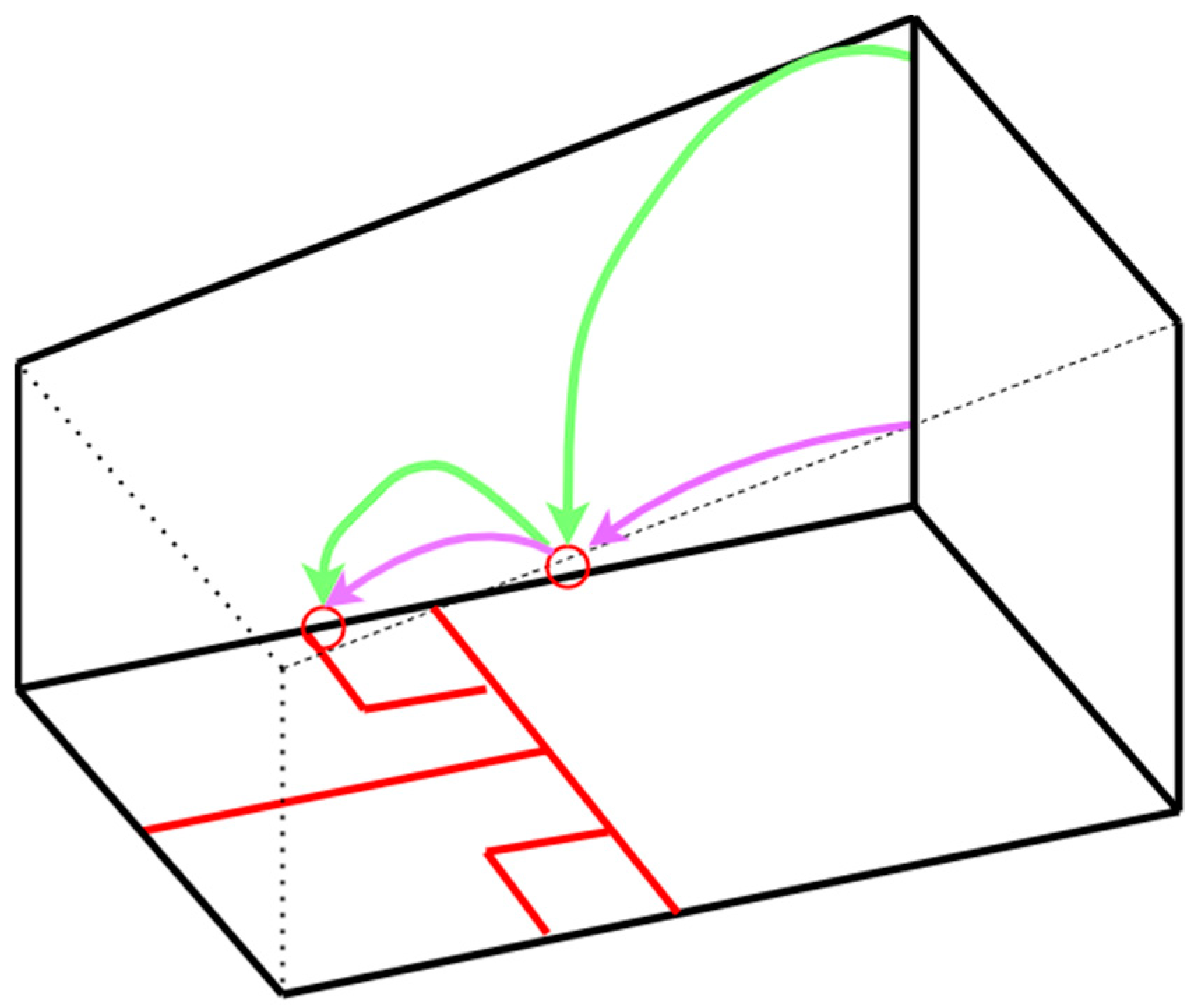

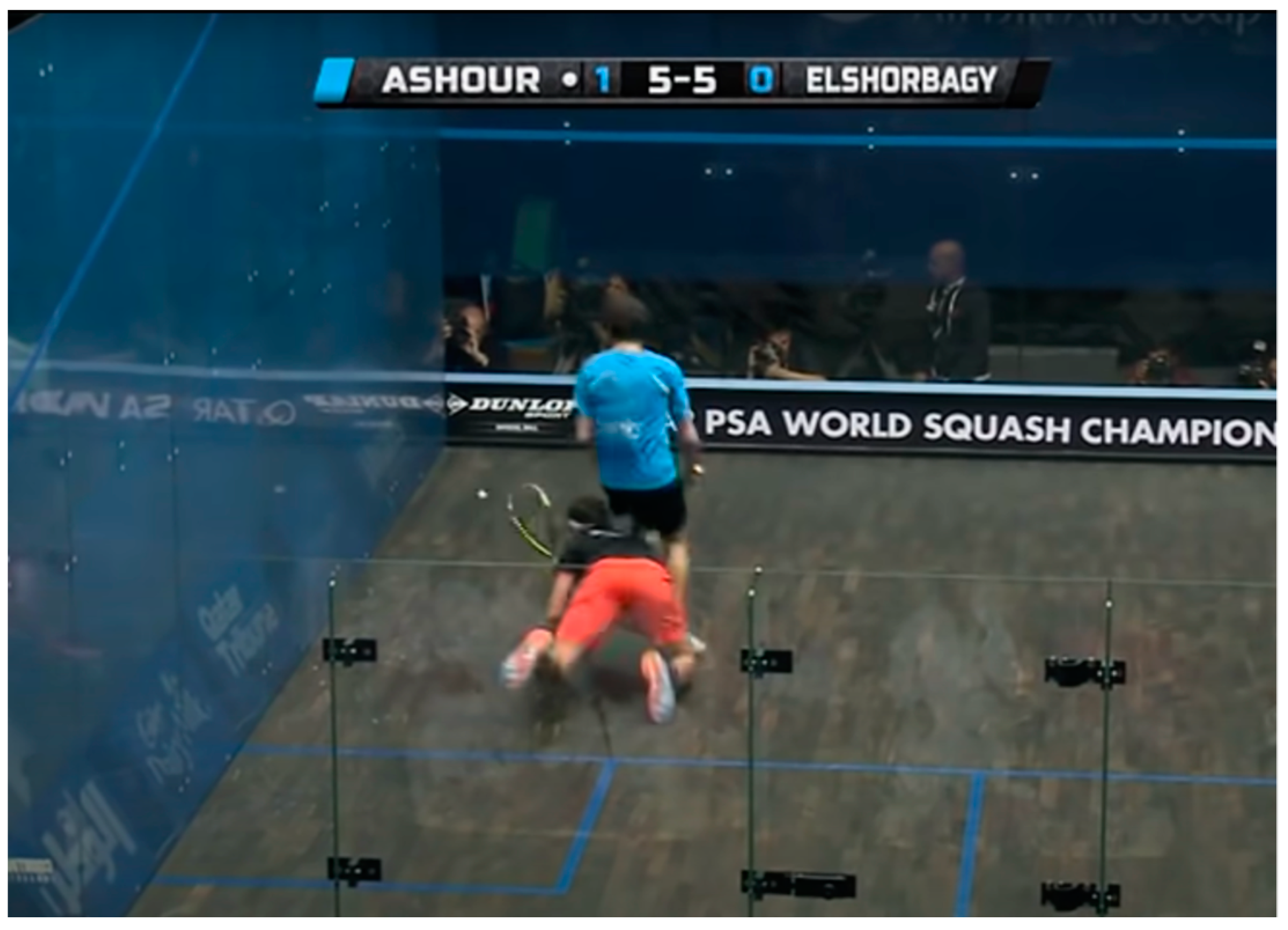
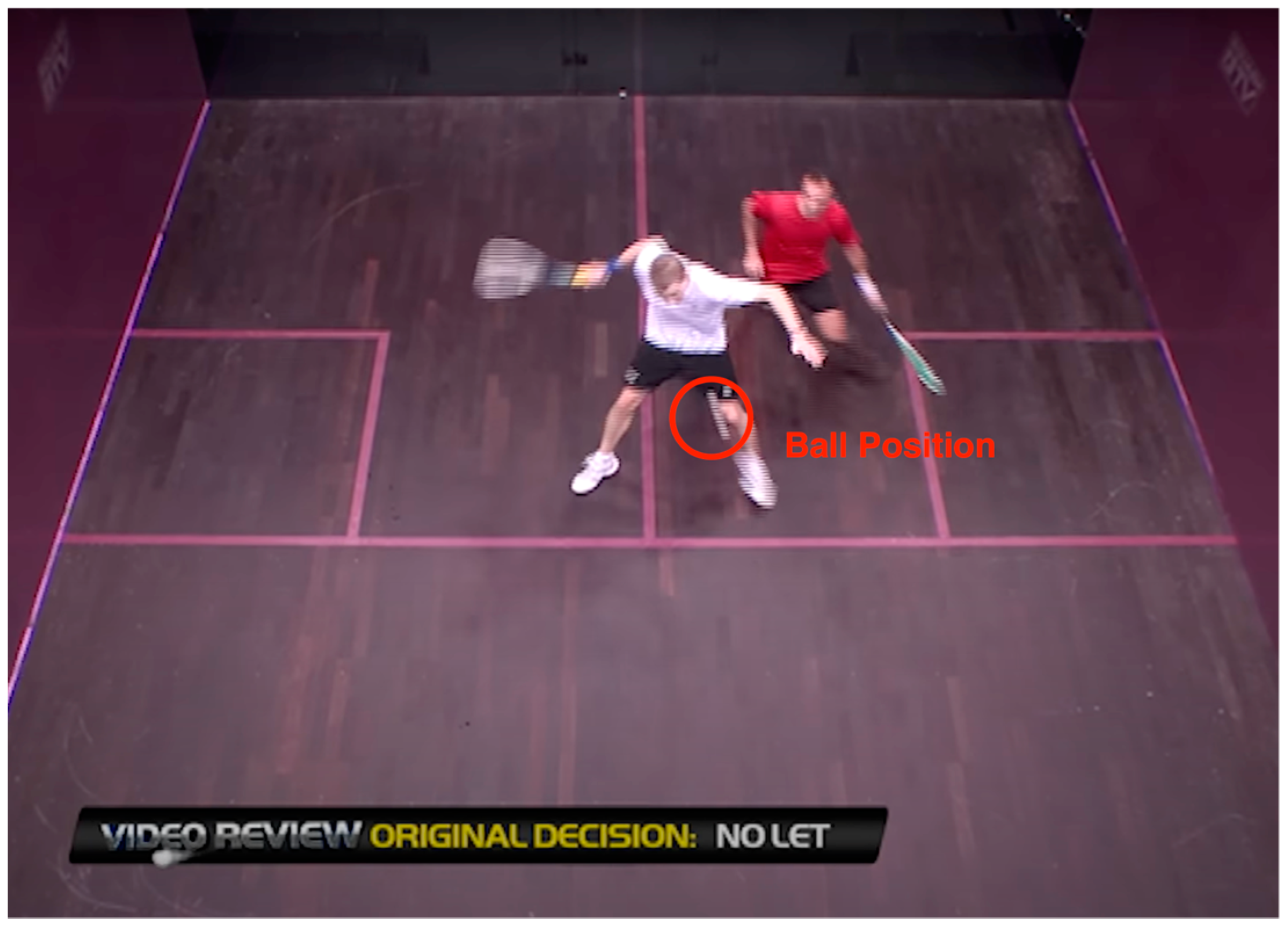

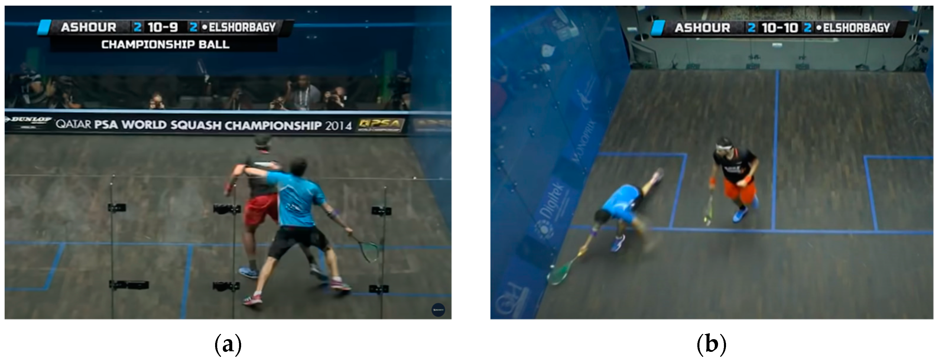
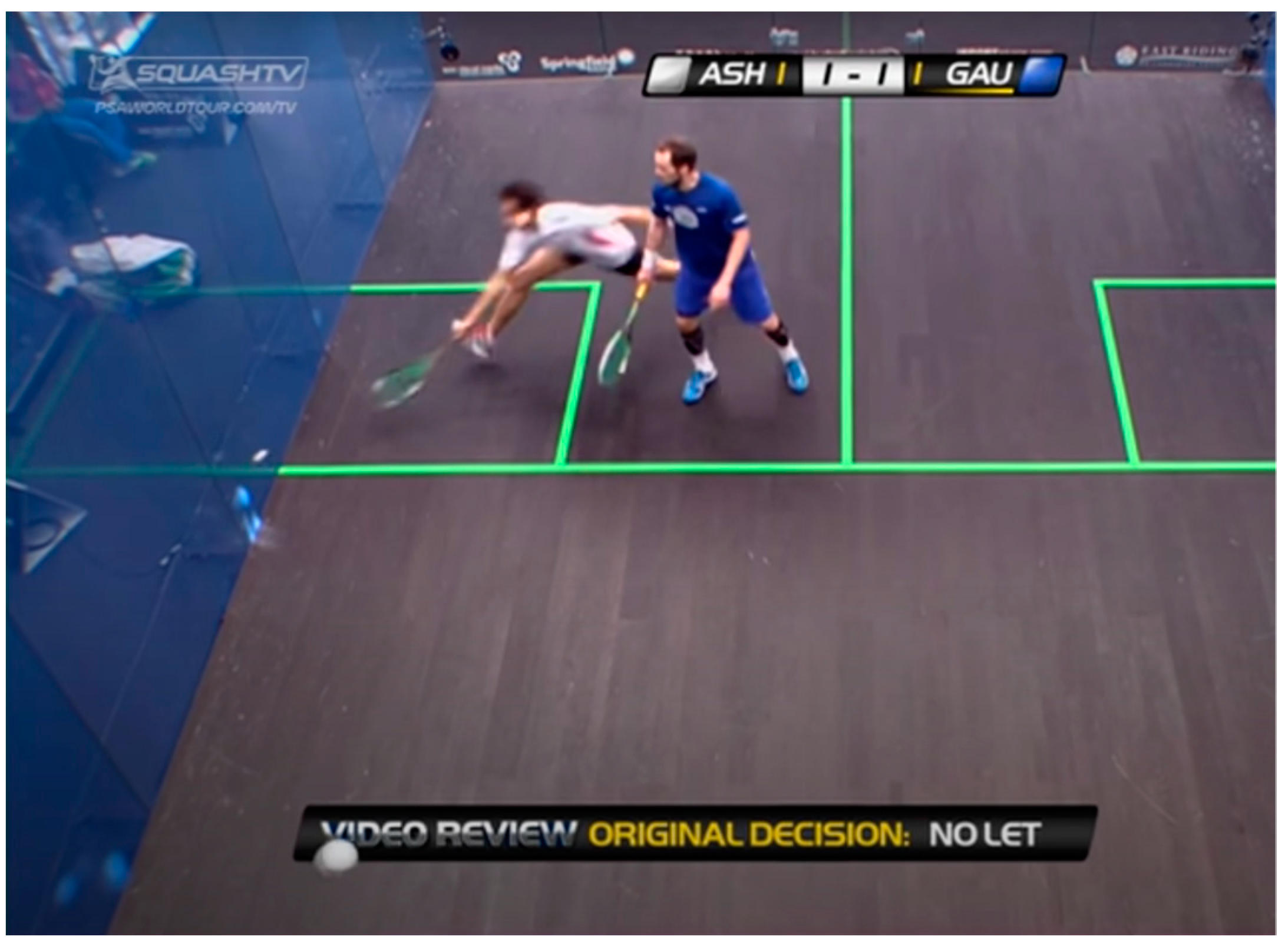


Disclaimer/Publisher’s Note: The statements, opinions and data contained in all publications are solely those of the individual author(s) and contributor(s) and not of MDPI and/or the editor(s). MDPI and/or the editor(s) disclaim responsibility for any injury to people or property resulting from any ideas, methods, instructions or products referred to in the content. |
© 2024 by the authors. Licensee MDPI, Basel, Switzerland. This article is an open access article distributed under the terms and conditions of the Creative Commons Attribution (CC BY) license (https://creativecommons.org/licenses/by/4.0/).