Classification, Regression, and Survival Rule Induction with Complex and M-of-N Elementary Conditions

Abstract

Most rule induction algorithms generate rules with simple logical conditions based on equality or inequality relations. This feature limits their ability to discover complex dependencies that may exist in data. This article presents an extension to the sequential covering rule induction algorithm that allows it to generate complex and M-of-N conditions within the premises of rules. The proposed methodology uncovers complex patterns in data that are not adequately expressed by rules with simple conditions. The novel two-phase approach efficiently generates M-of-N conditions by analysing frequent sets in previously induced simple and complex rule conditions. The presented method allows rule induction for classification, regression and survival problems. Extensive experiments on various public datasets show that the proposed method often leads to more concise rulesets compared to those using only simple conditions. Importantly, the inclusion of complex conditions and M-of-N conditions has no statistically significant negative impact on the predictive ability of the ruleset. Experimental results and a ready-to-use implementation are available in the GitHub repository. The proposed algorithm can potentially serve as a valuable tool for knowledge discovery and facilitate the interpretation of rule-based models by making them more concise.

1. Introduction

In knowledge discovery from tabular data, rules represent one of the most intuitive and widely used forms of knowledge representation. Many knowledge discovery problems can be considered as rule induction tasks. Examples of such tasks include association rule learning [1], subgroup discovery [2], contrast sets, and emerging patterns mining [3] and black-box explanation [4,5]. While the descriptive power of rules is widely acknowledged, they moreover find utility in predictive purposes (i.e., for building classification systems). The descriptive and predictive aspects of rule induction are closely related. In fact, any rule induction algorithm can be oriented toward one or both of these purposes. What distinguishes them are the strategies used to navigate the search space, the techniques used to evaluate the rules, and how they are subsequently refined.

For the purpose of knowledge discovery, the induction algorithm aims to find rules that fulfill assumed quality constraints, such as precision (confidence) or support (coverage). Subsequently, filtering can be applied based on the interestingness of the rule. If classification is the main goal, induction is oriented towards achieving the highest predictive power.

The vast majority of rule induction algorithms—some of which are listed in the Section 2—generate rules with premises consisting of simple elementary conditions. These conditions are expressed as $attribute\odot value$, where $\odot \in \{=,>,<,\ge ,\le \}$. While some algorithms permit the induction of negated conditions (e.g., $attribute\ne value$), only a few allow the induction of complex conditions. These complex conditions may involve comparisons of attribute values, M-of-N conditions, and conditions resulting from the use of constructive induction. The reliance on simple elementary conditions is a limitation of many rule induction algorithms. Rules with complex conditions can capture dependencies that cannot be represented using simple conditions.

Among the various rule learning approaches, the separate-and-conquer strategy (also known as sequential covering) represents a reasonable compromise, enabling the induction of a moderate number of rules with good predictive power. Importantly, the procedure can be easily tailored to the interpretability or classification abilities of the model by using different rule search strategies and rule quality criteria (quality measures).

In the articles [6,7], we demonstrated the effectiveness of our version of the sequential covering rule induction algorithm, confirming its performance across dozens of benchmark datasets. The algorithm is implemented in the RuleKit library [8].

The purpose and main contribution of this paper are to extend the RuleKit-based rule induction algorithm by introducing the capability to induce complex elementary conditions. Specifically, our original proposal involves generating M-of-N conditions based on the analysis of frequent sets constructed from both simple and complex (e.g., conditions comparing the values of two attributes) elementary conditions.

The proposed algorithm enables rule induction for classification, regression, and survival analysis problems. The conducted experiments show that the introduction of complex conditions does not significantly affect the predictive ability of rulesets. However, rules with complex conditions enable the description of data with a wider range of different dependencies.

The implementation of the algorithm is available on the GitHub repository (https://github.com/adaa-polsl/m-of-n-rules accessed on 21 February 2024). In addition, to ensure the reproducibility of the research, we have published detailed results of all the experiments conducted there.

2. Related Work

2.1. Rule Induction Algorithms

The earliest rule induction algorithms were based on the sequential covering strategy. This strategy involves constructing a set of rules by sequentially inducing rules that cover successive, not-yet-covered training examples. The sequential covering strategy was first proposed by Michalski [9], who presented several versions of the AQ algorithm [10,11,12,13]. Fürnkranz systematized the sequential covering approach to rule induction by analyzing the impact of rule specialization and generalization phases and rule search heuristics on the descriptive and predictive capabilities of induced rulesets [14,15].

Well-known sequential covering rule induction algorithms include AQ, CN2 [16], and RIPPER [17], but the family of such algorithms is extensive. AQ and CN2 generate sets of rules, while RIPPER generates a rulelist, which is important for the global interpretation of discovered dependencies and the method of example classification. LEM [18], DomLEM [19] and VC-DomLEM [20] exemplify rule induction algorithms combining the sequential covering idea with rough set theory.

Moreover, association rule induction algorithms can be used to induce classification rules [21,22]. In this approach, rule conclusions are fixed and always indicate a specific value of a decision attribute (class label). Rules that meet minimum confidence and minimum support requirements are generated, and a filtration algorithm is subsequently applied to eliminate redundant rules.

Another group somewhat related to the sequential covering strategy is the one based on ensemble classification approaches such as boosting [23,24,25], or bagging [26].

In recent years, several rule induction proposals based on optimizing a given loss function have been presented. Instead of inducing consecutive rules one by one, these algorithms optimize the entire ruleset according to a given loss function [27,28,29].

A growing number of proposals focus on extracting rulesets from trained neural networks [30,31,32,33]. Extracted rules are used not only for data description and prediction. They are applied to explain the decisions made by complex networks [30,32]. It is worth noting that effective rule induction algorithms based on neural network architectures were proposed over 20 years ago [34,35].

Recently, there has been a return to the idea of generating locally optimal rules for individual (specific) training examples. Although this approach usually yields better prediction results, it complicates understanding the decision-making mechanism. The idea of discovering locally optimal dependencies aligns with the fundamentals of rough set theory [36,37,38], where minimal decision rules are represented by local decision reducts. Examples of locally optimal rule induction algorithms not directly inspired by rough set theory are HARMONY [39] and LORD [40].

2.2. Learning Complex Elementary Conditions

Fundamentally, apart from some versions of AQ, all the aforementioned algorithms generate rules with simple elementary conditions ($a=v$, $a<v$, $a>v$; where a is a conditional attribute and v is one of its values). Some of these algorithms allow the induction of negated elementary conditions ($a\ne v$).

The AQ algorithm allows for the appearance of an internal disjunction in the elementary condition. The expression $a=v_1\vee v_2\vee \dots \vee v_n$ represents the elementary condition that has a form of internal disjunction. In this expression, a is a conditional attribute, and $v_1$, $v_2$, …, $v_n$ are specific values of a or intervals of a. A rule with an internal disjunction in its premise can be transformed into multiple (e.g., n) rules that contain only simple conditions.

Some approaches attempt to replace conventional attribute-value conditions with fuzzy intervals [41]. An example of such a method is the FURIA algorithm [42], which modifies RIPPER to induce fuzzy rules. FURIA tends to achieve better predictive accuracy than RIPPER but at the cost of generating more rules and conditions. Notably, fuzzification adds a layer of complexity to interpreting such rules, as it requires an awareness of the underlying fuzzy semantics.

Both classical and fuzzy rules can only determine axis-parallel decision boundaries. To overcome this limitation, some authors have proposed oblique decision rules. An oblique decision rule incorporates a linear combination of attributes in its premise. One example of such algorithms is CHIRA [43], which is a rule aggregation method that uses convex hulls to identify the regions covered by the aggregated rules and creates oblique elementary conditions based on them. Setiono and Liu [44] proposed a system capable of generating oblique decision rules from trained neural networks. Although oblique rules often can produce more compact and accurate rulesets, as they can handle more complex and non-linear relationships in data, they are less interpretable than conventional rules.

Much greater interpretability than fuzzy and oblique rules provides the induction of rules with M-of-N conditions. The M-of-N condition is represented as a disjunctive normal form (DNF) formula with N conjunctions, each containing M literals. For instance, the 2-of-3 condition can be written as a formula: $(w_1\wedge w_2)\vee (w_1\wedge w_3)\vee (w_2\wedge w_3)$, where $w_1$, $w_2$, $w_3$ are elementary conditions. However, the M-of-N condition may have various interpretations, such as “at least M out of N conditions are met”, “exactly M out of N are met”, and “at most M out of N conditions are met”. In addition, depending on the interpretation, the DNF formula representing the condition will differ. To induce the M-of-N conditions, greedy search [45,46], genetic algorithms [47], and constructive induction [48,49,50] have been applied. There are articles that present the idea of inducing M-of-N conditions from trained neural networks [51,52] and decision trees [50,53]. Some algorithms assume that the rule premise contains only M-of-N conditions. An analogy to the idea of inducing M-of-N formulas is found in the work by Beck et al. [54], proposing the induction of general logical functions by training alternating layers of conjunctive and disjunctive rulesets.

Considerations on various types of rule conditions are found in the [55] report, which is a kind of manifesto for the descriptive possibilities of classification (decision) rules. Although this work was written many years ago, to date, no broader research has been presented on the impact of complex elementary conditions on the descriptive and predictive capabilities of rulesets with such conditions. Moreover, there is no publicly available implementation of an algorithm generating complex conditions (e.g., enabling the comparison of attribute values or generating M-of-N conditions). It is worth noting that all the algorithms mentioned in this section apply only to classification problems.

Finally, we mention the studies related to introducing new attributes/features to the attribute set. New attributes reflect complex relationships between the basic attributes and can be generated using constructive induction methods (data-driven [56], hypothesis-driven [57], or other feature extraction methods [58]). Besides, new attributes may result from analyses (e.g., PCA [59], multidimensional scaling [60]) conducted by domain experts attempting to understand the dependencies present in the data of interest [61]. Although constructive induction may influence the descriptive and predictive capabilities of generated rulesets, it is only somewhat related to our article. Our method of inducing M-of-N conditions can be particularly viewed as an implementation of the concept of constructive hypothesis-driven induction.

3. Methods

3.1. Basic Notion

Let us consider the dataset $D(A,\delta )$, which contains $\left|D\right|$ examples. Each example is described using a fixed set of attributes $A=\{a_1,a_2,\dots ,a_{\left|A\right|}\}$ and a special decision attribute $\delta$. The form and interpretation of decision attributes can vary based on the type of problem specified. In this paper, we focus on three problem types: classification, regression, and survival analysis.

For the classification problem, each example could be assigned to a specific class based on the value of the decision attribute. In such a case, $\delta$ is a discrete class identifier $\delta \in \{L_1,L_2,\dots ,L_{\left|L\right|}\}$. The task involves predicting the correct class value $L_j$ for a given example $X_i$. In a regression problem, the decision attribute is a continuous variable: $\delta \in \mathbb{R}$. Therefore, the task is to predict its value with minimal error, ideally zero. In survival analysis, the label attribute refers to the Boolean censoring status, indicating whether the example was subject to a certain event (e.g., patients who suffered a stroke). For such an analysis, an additional survival time attribute T is required. The attribute T specifies the time before the event occurs, if the event occurs, for a given example. Otherwise, it equals the overall observation time. For classification and regression data, each example from D is represented as a vector $x_i=(a_{i1},a_{i2},\dots ,a_{i\left|A\right|},{\delta }_i)$. For the survival problem, this vector must be extended by the variable $T_i$.

Our main objective is to define (induce) a set of rules describing examples from the set D and enabling the prediction of the value of the attribute $\delta$ for new (unseen) examples. This set of rules is later referred to as a rule-based data model.

Let R be a set of $\left|R\right|$ rules. Each rule $r\in R$ takes the following form:

$$\mathbf{IF}{c}_1\wedge c_1\wedge \dots \wedge c_n\mathbf{THEN}\delta =f\left(X\right).$$

The rule premise is a conjunction of elementary conditions $c_i$ ($i\in 1,2,\dots ,n$).

If an example x fulfills the conditions of a rule r premise, we say that r covers x (x is covered by r).

The conclusion of a rule contains the decision part used during the prediction process. For classification and regression rules, a constant function is defined specifying a certain value of the decision attribute $\delta$ (e.g., a certain decision class).

For a survival rule r, $f\left(x\right)$ represents the Kaplan–Meier [62] estimator (i.e., the survival curve) defined based on all examples covered by r.

A set of rules can be treated as a predictor. The prediction is made by evaluating the premise part of each rule for a given example x. Only the rules covering the example x participate in the prediction process. The predicted value is obtained based on the decision part of these rules. If all rules covering the example x have the same conclusion, the prediction is straightforward. The predicted value of the decision attribute of example x is taken from the conclusions of the rules.

For classification problems, if an example is covered by rules with different conclusions, a voting procedure is invoked. Each rule covering the given example votes for the predicted value from its conclusion, and each vote is multiplied by the so-called voting weight. Voting weights can be calculated in various ways, such as using rule quality measures [8,63].

In regression and survival problems, the final prediction is obtained by averaging the decisions of the rules covering the example. In particular, in survival analysis, the Kaplan–Meier estimators of all rules covering a given example are averaged to obtain the final prediction value.

Another scenario is applied to an example not covered by any rule. Such an example is usually predicted using the so-called default rule. The premise of the default rule is empty, ensuring that the default rule covers every example. The conclusion of the default rule is calculated for the entire set of training examples and specifies the majority class for classification problems, the median value of the decision attribute for regression problems, and the Kaplan–Meier estimator for survival data.

Most existing rule induction algorithms generate rules with simple elementary conditions. The simple elementary condition has one of the following forms: $a=v$ or $a<v$ or $a>v$, where a is a conditional attribute, and v is one of its values. Such conditions may not always be optimal for describing datasets containing more complex relationships. In this paper, we focus on the induction of rules containing more complex conditions. We consider the following types of complex conditions.

• Negated conditions: Represent negations of simple conditions (e.g., $a\ne v$, $a\notin [v_1,v_2)$ and all complex conditions listed below (except Disjunctions).
• Attribute Relations: This type of condition covers all examples for which a given relation exists between given attributes. They are generated only for attributes of the same type, either nominal or numeric. For nominal attributes, the possible relations are equality and inequality. For numeric ones, the relations of strict and weak inequalities are additionally analyzed. Examples of such conditions are presented below:

  $$a=b,a\le b\mathrm{where}a\mathrm{and}b\mathrm{are}\mathrm{attributes}.$$
• Internal Disjunctions: For nominal attributes, an elementary condition with internal disjunction is defined as follows:

  $$a\in \{v_1,v_2,\dots ,v_k\}\mathrm{where}{v}_1,v_2,\dots ,v_k\mathrm{are}\mathrm{values}\mathrm{of}a.$$

  For numeric attributes, the internal disjunction is represented as a disjunction of mutually disjoint intervals of values of the attribute a:

  $$a=([v_1,v_2)\vee [v_3,v_4)\vee \dots \vee [v_5,v_6)),$$

  where $v_1$ < $v_2$ <, …, < $v_k$ are values of a.
  The above expression can be rewritten as an alternative of the simple elementary conditions $a=v_i$, ($i\in \{1,2,\dots ,k\}).$

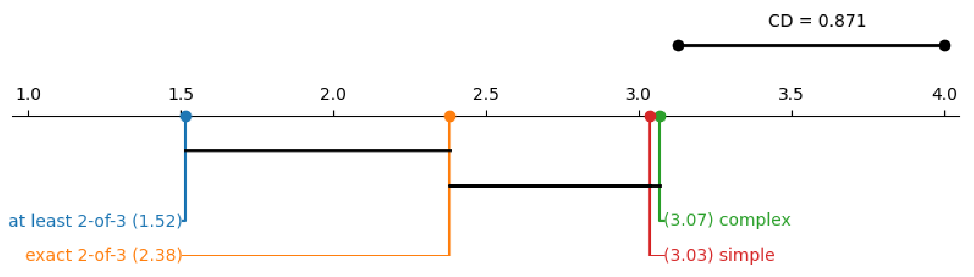
In this article, we propose a methodology that allows the induction of conditions known as M-of-N conditions. An M-of-N condition consists of N conditions, which can be either simple or complex. In our study the M-of-N condition is satisfied if exactly M or at least M of its N components are satisfied. Depending on the interpretation of the M-of-N condition, the sets of examples covering this condition may vary. In the experiments, we considered both interpretations of the M-of-N condition. An example of the M-of-N condition (2-of-3 condition) is presented below.

$$2-of-3(a=b,a\ne v,c\in \{v_1,v_2,v_3\}).$$

We can say that an M-of-N condition represents a compressed form of the DNF formula consisting of N disjunctions, each of which has M literals.

To simplify the notation, we denote all N conditions that are part of M-of-N by $C^{\prime }=\{c_1,c_2,\dots ,c_l\}$. In the case of our example, $C^{\prime }=\{c_1,c_2,c_3\}$. Using such a notation, the DNF form of our example condition, for the “at least M-of-N” interpretation, is as follows:

$$(c_1\wedge c_2)\vee (c_1\wedge c_3)\vee (c_2\wedge c_3).$$

For the “exactly M-of-N” interpretation, the DNF form of our example is as follows:

$$(c_1\wedge c_2\wedge \neg c_3)\vee (c_1\wedge c_3\wedge \neg c_2)\vee (c_2\wedge c_3\wedge \neg c_1).$$

3.2. Learning Rules with Simple Conditions

To induce rules with simple conditions, our approach employs the sequential covering rule induction algorithm. This algorithm makes it possible to induce classification, regression, and survival rules. The source code for the algorithm is available on GitHub [8] as the RuleKit library. In this subsection, we provide a concise explanation of RuleKit for all three types of rules. For a comprehensive understanding of how the RuleKit algorithm works, refer to [6,7] and the library documentation [64].

The algorithm starts with an empty ruleset and iteratively learns a single rule to induce a ruleset that covers the entire set of training examples, or until the number of uncovered examples remains below some fixed (algorithm’s parameter) value. After the induction of a rule, all examples covered by the rule are removed from the training set, and the algorithm proceeds to induce the next rule, which covers some of the remaining examples.

Inducing a new rule involves two phases: rule growing and rule pruning. In the growing phase (Algorithm 1), elementary conditions are added to the initially empty premise. When extending the premise, the algorithm considers all possible conditions built upon all attributes (line 5: GETALLCONDITIONS function call) and selects those leading to the rule with the highest quality. The algorithm enables the use of any well-known rule quality measures [63] or a user-defined rule quality measure. These measures guide the rule induction process, favoring rules that cover as many positive and few negative examples as possible. Using the rule quality measure, the algorithm aims to maximize the number of positive examples while minimizing the number of negative ones covered by the induced rules.

In the simplest version of the algorithm, the function GETALLCONDITIONS generates a set of all possible simple elementary conditions. For nominal attributes, conditions in the form $a_i=v_i$ for all values $v_i$ from the attribute domain are considered. Regarding continuous attributes, $v_i$ values present in the observations covered by the rule are sorted. Subsequently, potential split points $s_j$ are determined as the arithmetic means of subsequent $v_i$ values, and conditions $a_i<s_j$ and $a_i\ge s_j$ are evaluated. If multiple conditions yield identical results, the one covering more examples is chosen. Rule pruning can be considered the opposite of rule growing. It iteratively removes conditions from the premise, systematically making eliminations that lead to the most substantial improvement in rule quality. The procedure stops when no conditions can be deleted without diminishing the rule’s quality or when the rule contains only one condition. RuleKit uses the hill climbing strategy for both rule growth and pruning. The process of searching for the best conditions is illustrated in Algorithm 2.

In the classification problem, the algorithm systematically iterates over all decision classes (class labels). In regression and survival analysis problems, the algorithm is executed once on the entire set of training examples. In the case of a regression problem, RuleKit transforms it into a binary classification problem, following the proposal in [65]. The conclusion of a regression rule r indicates a specific value of the decision attribute $\delta$. This value is calculated as the median $Me$ of the decision attribute values of the examples that cover r. All training examples with a value $\delta$ within a range $[Me-\sigma ,Me+\sigma ]$ represent the positive decision class, while the remaining examples represent the negative one. It is important to note that changing the premise of an induced rule dynamically affects the class membership of the covered examples. For survival analysis, RuleKit, instead of relying on rule quality measures, uses the log-rank test [66] to evaluate a rule during the growth and pruning phases. This test compares the differences between two Kaplan–Meier estimators: one fitted to the examples covered by the rule and the other fitted to the remaining examples.

3.3. Rules with Complex Conditions

The induction of rules with complex conditions (excluding M-of-N) is very similar to to the induction of rules containing only simple conditions.

When inducing rules with complex conditions, the set of all possible conditions (GETALLCONDITIONS line 5) includes not only simple conditions but in addition all possible attribute relations, internal disjunctions for symbolic attributes, and negated conditions.

The algorithm considers all possible attribute relations for attributes of the same type. For a symbolic attribute, the set of internal disjunctions corresponds to the power set of the attribute values.

To avoid nonsensical comparisons for a given dataset and to reduce computational complexity, the algorithm utilizes a list of attributes that should not be compared and limits the number of values that an internal alternative can contain.

Compared to the standard version of the RuleKit algorithm, the rule-growing phase differs only when internal disjunctions based on numeric attributes are added to the rule premise. The main modification involves introducing additional steps (see lines 8–10) into Algorithm 1. These additional steps occur only if the best-selected condition found earlier (line  6) is based on the numeric attribute. The GETDISJUNTIONS procedure extends this condition with pairs of mutually disjoint intervals.

The rule pruning phase remains the same as in the original version of the RuleKit algorithm. In both phases, there is a change in the selection of the best condition when several conditions achieve the same quality.

Algorithm 1 Rule growing

Require:   D—training dataset,   $D_u$—uncovered set of examples,   $D_r$—examples covered by r,   T—list of condition types to induce. Ensure: r—rule. 1:  function Grow(D,$D_u$, T) 2:   $r\leftarrow \varnothing$ 3:   repeat 4:    $D_r\leftarrow$Covered(r, D) 5:    $C\leftarrow$GetAllConditions(T, D, $D_r$, $D_u$) 6:    $c_{best}\leftarrow$GetBestCondition(C, r, D) 7:    ▹ induce internal disjunctions for numeric attributes 8:    if $c_{best}\ne \varnothing \wedge$ T includes INTERNAL_DISJUNCTIONS then 9:     $C_{alt}\leftarrow$GetDisjunctions($c_{best}$, D, $D_r$, $D_u$) 10:     $c_{best}\leftarrow$GetBestCondition($\left\{c_{best}\right\}\cup C_{alt}$, r, D) 11:    if $c_{best}\ne \varnothing$ then 12:     $r\leftarrow r\wedge c_{best}$ 13:   until $c_{best}\ne \varnothing$ 14:   return r

To compare the quality of elementary conditions, a lexicographic order is used. Let us suppose that a condition c is given and a rule r contains c in its premise, then the condition c is evaluated according to the following criteria (see Algorithm 2):

• The quality of r—line 6;
• The number of positive examples covered by r—line 9;
• The number of unique attributes included in c—line 11;
• Comprehensibility, complexity of c—line 15.

The last criterion reflects our subjective assessment of the comprehensibility of elementary conditions. Each type of elementary condition is assigned a weight that reflects its comprehensibility:

• Simple Conditions, Negated condition: 1;
• Attribute Relation: 2;
• Internal Disjunction:

  –

  For numeric attributes: 0;

  –

  For symbolic attributes 2.

The higher the weight value, the more comprehensible the condition. It should be emphasized that the last criterion is invoked only when the conditions being compared achieve the same evaluation for the remaining criteria.

Algorithm 2 Finding the best condition

Require:   C—set of conditions,   r—rule,   D—training dataset. Ensure: $c_{best}$—best condition. 1: function GetBestCondition(C,r,D) 2:   $c_{best}\leftarrow \varnothing$, $q_{best}\leftarrow -\infty$     ▹ best condition and its quality 3:   for $c\in C$ do 4:    $r_c\leftarrow r\wedge c$           ▹ add condition to the rule 5:    $q\leftarrow$CalculateQuality($r_c$, D) 6:    $found\_better\leftarrow (q>q_{best})$     ▹ compare quality 7:    if $\neg found\_better\wedge q=q_{best}$ then 8:     ▹ prefer conditions with a higher coverage 9:     $found\_better\leftarrow$ (CoveredCount(c, D) > CoveredCount($c_{best}$, D)) 10:     if $\neg found\_better$ then 11:      ▹ prefer conditions with a smaller number of attributes 12:      $found\_better\leftarrow$ (AttributesCount(c) < AttributesCount($c_{best}$)) 13:      if $\neg found\_better$ then 14:        ▹ prefer conditions types with a higher weight 15:        $found\_better\leftarrow$ (TypeWeight(c) > TypeWeight($c_{best}$)) 16:    if $found\_better$ then 17:     $c_{best}\leftarrow c$, $q_{best}\leftarrow q$ 18:   return $c_{best}$

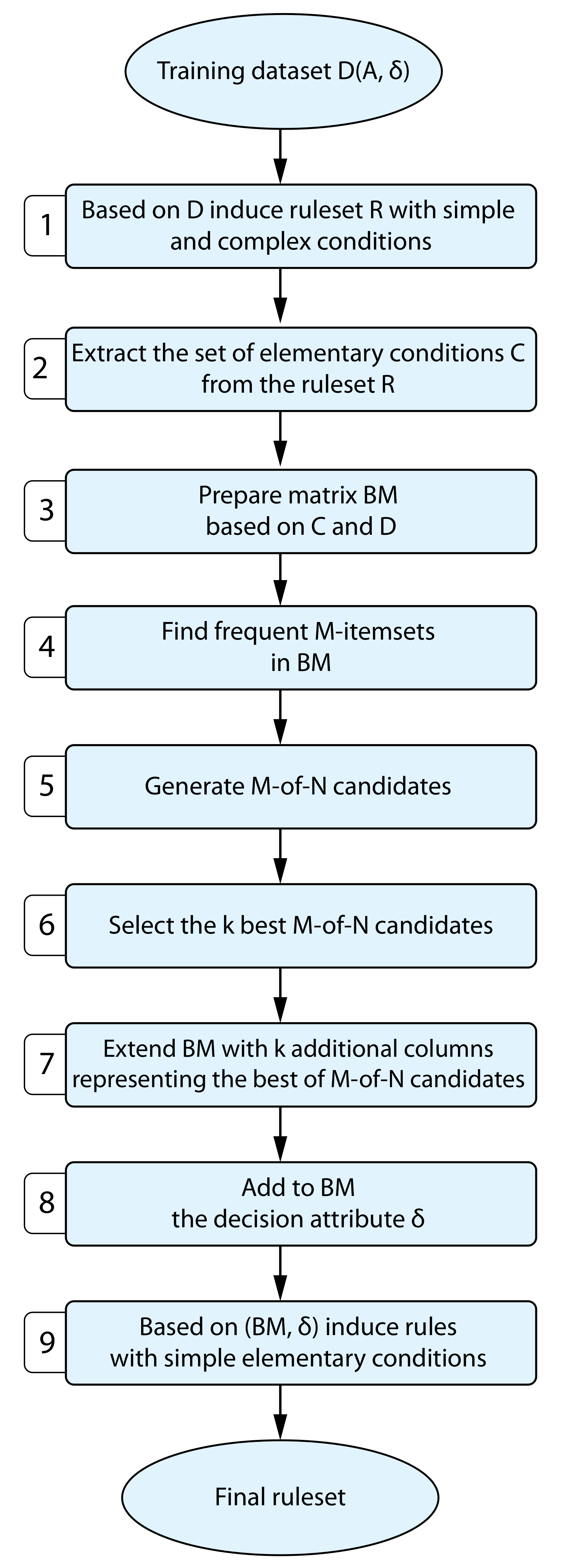
3.4. Learning Rulesets with M-of-n Conditions

The method for inducing rules with M-of-N conditions assumes that these conditions are constructed based on an already-induced set of rules (R). The set R contains rules with both simple and complex conditions (Block 1—Figure 1). Following rule induction, a set C containing all elementary conditions present in ruleset R is determined (Block 2, Figure 1). In the subsequent step, a table—binary matrix ($BM$)—is constructed, with each column (k) representing an elementary condition from C (Block 3, Figure 1). The matrix $BM$ contains |C| columns and |D| rows, each row representing one training example. For a given training example $x\in D$ and column $k\in BM$, $k\left(x\right)=1$ if and only if x is covered by an elementary condition represented by column k; otherwise, $k\left(x\right)=0$. 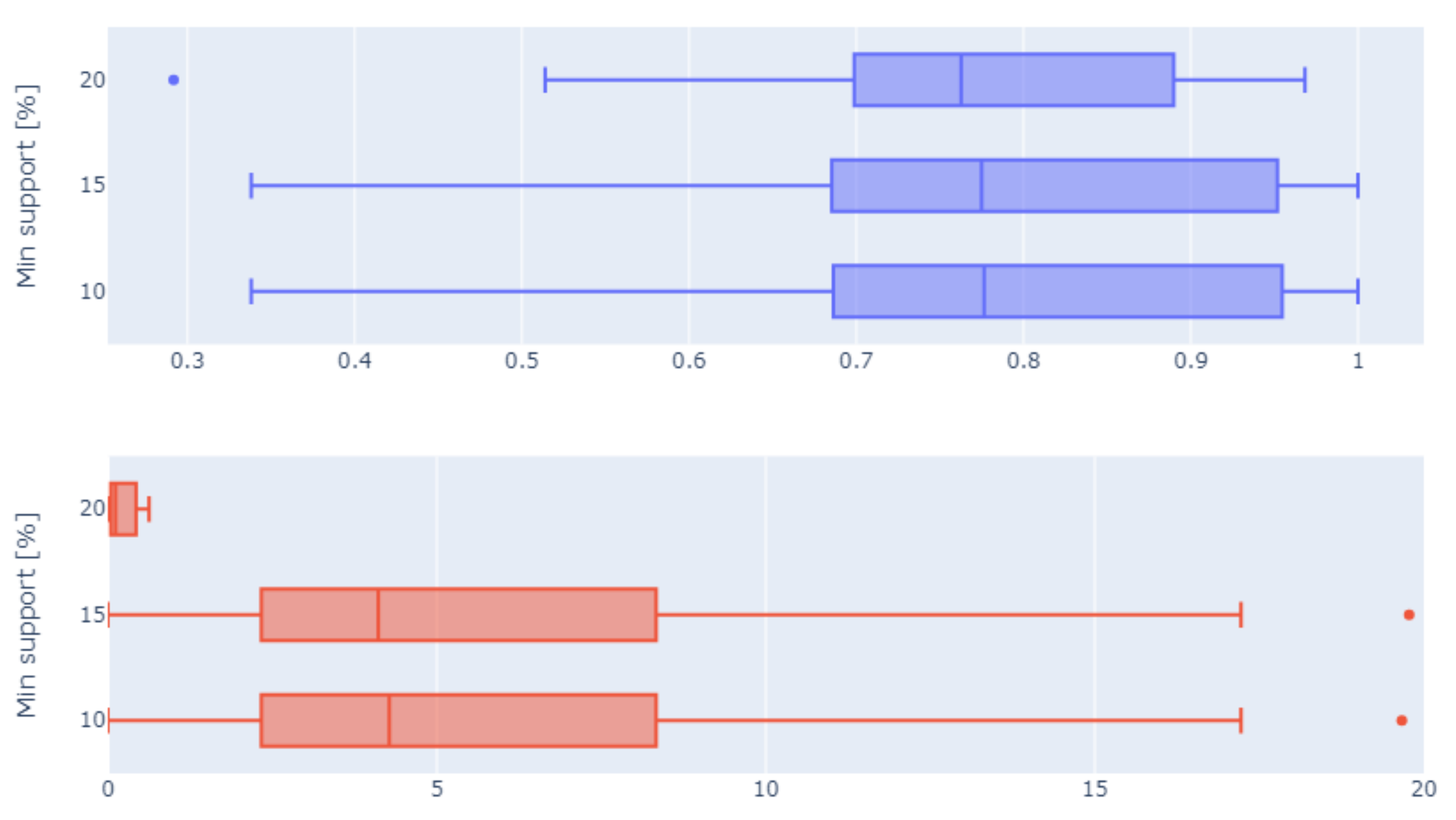In $BM$, frequent sets fulfilling the minimum support condition (algorithm’s parameter) are mined. Specifically, for all allowed values of M, all frequent M-itemsets are mined. For instance, if the analysis aims to extend the set of elementary conditions with 2-of-3 and 3-of-4 conditions, both frequent 2-itemsets and 3-itemsets are sought. In the proposed method, the FP-growth algorithm [67] is applied to mining frequent itemsets. Following frequent itemset mining, the procedure to generate candidates for M-of-N conditions is initiated (Block 4, Figure 1). A candidate for the M-of-N condition comprises N frequent M-itemsets (see Example). To constrain the number of candidates in further calculations, the average support is calculated for each M-of-N candidate. The average support of an M-of-N condition is the average value of supports of all N frequent M-itemsets defining this condition. The top l (algorithm’s parameter) candidates with the highest support are selected for further processing. In the penultimate step, the binary matrix $BM$ is extended with l candidate M-of-N conditions (Block 5, Figure 1). To the extended $BM$ matrix, a decision column identical to the one in the training set D is added (Block 6, Figure 1). Finally, the rule induction is performed on ($BM$, $\delta$), but this time the rule induction algorithm induces rules only with simple elementary conditions (i.e., $k=1$ or $k=0$). Note that column k in the extended $BM$ matrix may represent a simple, complex (created in Block 2, Figure 1) or M-of-N condition (created in Block 4, Figure 1).

The proposed method has an additional advantage: if an induced rule contains a condition $k=0$, and for example, k corresponds to the M-of-N condition, this means that the rule contains the negation of M-of-N.

• Example
• Let us assume that D contains a nominal attribute a and two numeric attributes b and c. The ruleset induced in the first step contains the following conditions: $a=1$, $a=0$, $a=2$, $b>2$, $b>5$, $b<4$, $b=c$. The matrix BM contains 7 columns. Moreover, let us assume that 2-of-3 conditions are induced and the FP-growth algorithm found the following frequent 2-itemsets, fulfilling the minimal support requirement:
  • $\{a=0,b<4\}$;
  • $\{a=0,b=c\}$;
  • $\{b<4,b=c\}$.
  These itemsets may define a single 2-of-3 condition candidate:

  2-of-3 (a = 0, b < 4, b = c).

4. Experiments and Results

4.1. Experiments Methodology

To evaluate the proposed methods, experiments were carried out on 76 publicly available datasets. Among all the considered datasets, 25 contain only numeric attributes, comprising 7 for classification, 12 for regression, and 6 for survival analysis. Another 12 datasets consist solely of symbolic attributes, with 11 being classification datasets and 1 for regression. The remaining datasets contain both symbolic and numeric attributes. The aggregated statistics of the datasets are presented in

Table 1. Statistics of the datasets used during experiments.

Problem Type	Number of Datasets		Attributes		Rows
	All	with Missing Values	Mean	Min/Max	Mean	Min/Max
Classification	30	10	16	4/61	1131	101/12,960
Regression	30	3	9	3/28	189	27/625
Survival	16	7	16	6/57	723	187/3154

. All results, source code, and detailed characteristics of these datasets are available in the GitHub repository (https://github.com/adaa-polsl/m-of-n-rules accessed on 21 February 2024). All experiments were carried out in a stratified 10-fold cross-validation mode, with the exception of the Monk’s datasets, where the default division into training and testing parts was used.

For each dataset, four rulesets were trained. The first, denoted as simple contains only simple elementary conditions. The second, denoted as complex, contains complex and simple conditions, and the last two rulesets, at least M-of-N and exactly M-of-N, contain simple, complex, and M-of-N conditions, reflecting two interpretations of these conditions.

During rule induction, the well-known $C2$ rule quality measure [6,68] (see Equation (1)) was used in the rule growing and pruning phases, and for classification conflicts resolution. We decided to use this measure because it favors rules with high precision and moderate coverage [6,7]. Moreover, each new rule added to the ruleset had to cover at least two previously uncovered positive examples. Following the completion of the growing phase, a rule had to cover at least five examples, unless the total number of positive examples in the analyzed dataset was fewer. This allows the algorithm to induce rules even for datasets with very small decision classes containing only a few examples, while avoiding overly specific rules covering individual data entries. Induced rulesets were not required to cover the entire dataset: a maximum of 2% of the examples could remain uncovered by any rule. Such a configuration allows us to disregard a certain level of outlier examples in the training dataset.

$$C2=Coleman·\frac{P+p}{2P}\mathit{where}Coleman=\frac{Np-Pn}{N(p+n)}$$

(1)

When searching for frequent itemsets, the minimal support value was set at 0.2. Before selecting this value, we tested three minimal support values: 0.1, 0.15, and 0.2 (refer to the Section 4.2 for more details).

For all experiments involving the induction of M-of-N conditions, only the 2-of-3 conditions were induced.

For rulesets evaluation, we used the standard metrics:

• Classification: balanced accuracy (BAcc);
• Regression: relative root-mean-squared error (RRMSE (2));
• Survival: integrated Brier score [64] (IBS (3) and (4) [69]).

$$RRMSE=\frac{\sqrt{\frac{1}{n}{\sum }_{i=1}^n{(y_i-\overline{y})}^2}}{\frac{{\sum }_{j=1}^n{y}_j}{n}}$$

(2)

$$IBS={\int }_{t_0}^{t_{max}}B{S}^c\left(t\right)dw\left(t\right)$$

(3)

$${\mathrm{BS}}^c\left(t\right)=\frac{1}{n}\sum _{i=1}^{n}I(y_i\le t\wedge {\delta }_i=1)\frac{{(0-\hat{\pi }\left(t\right|{\mathbf{x}}_i))}^2}{\hat{G}\left(y_i\right)}+I(y_i>t)\frac{{(1-\hat{\pi }\left(t\right|{\mathbf{x}}_i))}^2}{\hat{G}\left(t\right)}$$

(4)

To evaluate the quality of induced rules, both precision ($p/(p+n)$) and coverage ($p/P$) were calculated. For the survival problem lacking defined decision classes, the rule support ($\left|r\right|/\left|D\right|$) is reported. In the aforementioned expressions, p and n denote the number of positive and negative examples covered by a rule, respectively; P denotes the total number of positive examples; $\left|D\right|$ represents the total number of examples; and $\left|r\right|$ denotes the number of examples covered by the rule r.

In addition, quantitative analysis of the results included assessing the statistical significance of the induced rules. The fraction of significant rules in the ruleset was calculated as the fraction of rules with a p-value less than 0.05. The p-values were calculated as follows:

• For classification: using Fisher’s exact test to compare confusion matrices;
• For regression: using the ${\chi }^2$ test to compare label variance for covered and uncovered examples;
• For survival: using the log-rank test to compare survival estimators for covered and uncovered examples.

All p-values were corrected using false discovery rate (FDR) correction [70].

4.2. Results

Table 2. Characteristics of classification rulesets.

Conditions	Rules Count	Conditions Count			Precision	Coverage	Fraction of Significant Rules
		Simple	Complex	M-of-N
Simple	60.8	2.8	-	-	0.96	0.14	0.94
Complex	44.2	1	1.5	-	0.96	0.16	0.94
Exactly 2-of-3	43.4	1.4	0.8	0.2	0.95	0.16	0.94
At least 2-of-3	43.8	1.4	0.9	0.2	0.96	0.16	0.94

,

Table 3. Characteristics of regression rulesets.

Conditions	Rules Count	Conditions Count			Precision	Coverage	Fraction of Significant Rules
		Simple	Complex	M-of-N
Simple	20.8	2.8	-	-	0.76	0.14	0.51
Complex	21.9	0.6	2.9	-	0.83	0.13	0.69
Exactly 2-of-3	15.9	1.3	1.2	0.6	0.81	0.21	0.53
At least 2-of-3	14.6	1.4	1.3	0.3	0.82	0.22	0.54

and

Table 4. Characteristics of survival rulesets.

Conditions	Rules Count	Conditions Count			Support	Fraction of Significant Rules
		Simple	Complex	M-of-N
Simple	7.8	2.2	-	-	0.37	0.95
Complex	11.1	1.1	3.4	-	0.29	0.94
Exactly 2-of-3	6.4	0.9	1.3	1.0	0.37	0.97
At least 2-of-3	5.3	0.9	1.2	0.6	0.42	0.98

present average values of the statistics characterizing induced rulesets. Detailed results, separately for all datasets, are available in the GitHub repository (https://github.com/adaa-polsl/m-of-n-rules accessed on 21 February 2024).

Upon analyzing the aforementioned table, one may observe that rulesets containing complex and M-of-N conditions, in general, contain a lower number of rules than rulesets with simple conditions. The only exception is in survival data, where rulesets containing complex conditions have the most rules. Classification rules have similar precision and coverage. In comparison to rules with simple conditions, regression rules with M-of-N conditions have higher precision and coverage. Regression rules with complex conditions are the most specific because they have the highest precision and the lowest coverage. A similar relationship is observed for survival rules with complex conditions, which have the lowest support. This low support is the reason for the higher number of induced rules.

The fraction of significant rules in the rulesets is very similar. For classification and survival rules, almost all induced rules are statistically significant, while for regression rules, only 50% of rules are significant. However, the introduction of complex and M-of-N conditions to the rule premises does not negatively affect the percentage of rules that are significant. Rulesets with complex conditions contain rules of the highest precision, leading to a larger number of statistically significant rules in these sets.

In analyzing the values in the ‘Conditions count’ columns, one may observe that the introduction of complex conditions into rule premises results in this type of condition becoming the most prevalent. However, when permitting the induction of M-of-N conditions, the occurrence of simple and complex conditions becomes comparable. There are only a few M-of-N conditions in the induced rulesets. This is because the $min\_supp$ value for acceptable frequent itemsets was set to 0.2 (subsequent sections present results for other $min\_supp$ values). Both interpretations of the M-of-N conditions yield similar outcomes. Rulesets containing M-of-N conditions have slightly higher coverage compared to other rulesets, along with marginally greater (in regression) or comparable (in classification) precision.

Figure 2, Figure 3 and Figure 4 show the results of the statistical analysis comparing the number of induced rules. In this comparison, the Friedman test and Nemenyi post hoc test (with a significance level of 0.05) were conducted [71]. The presented critical difference (CD) diagrams show the differences between different versions of the algorithm. Specifically, they show that there are no differences between rulesets with simple and complex conditions or between rulesets with complex and M-of-N conditions. However, it is worth noting that the test used is very conservative. When examining the algorithm rankings, it is evident that rulesets containing M-of-N conditions are the least numerous, regardless of the type of training data considered.

Table 5. Prediction results on test datasets (10-fold CV).

Conditions	BAcc	RRMSE	IBS
Simple	0.771 ± 0.077	0.728 ± 0.234	0.179 ± 0.036
Complex	0.774 ± 0.079	0.794 ± 0.344	0.185 ± 0.038
Exactly 2-of-3	0.758 ± 0.084	0.782 ± 0.344	0.188 ± 0.05
At least 2-of-3	0.756 ± 0.085	0.787 ± 0.336	0.186 ± 0.05
Decision tree	0.76 ± 0.199	0.82 ± 0.282	0.21 ± 0.0701

shows the prediction possibilities of the induced rulesets. The rule induction algorithm with simple elementary conditions attains the highest balanced accuracy and the lowest RRMSE and IBS values. In analyzing the contents of Table 5, one can notice that all rulesets achieve similar results. For the classification problem, the complex variant is better than the others, while the variants that introduce N-of-N conditions achieve slightly worse results than the simple one. The regression rulesets obtain very similar results, except for the ruleset with simple conditions, which attains the best result. A very similar situation is observed for survival rules.

For a more insightful comparison of the tested rulesets, the Friedman test with and without FDR correction was run (

Table 6. Friedman’s tests results (p-values).

	Rules Count		Prediction Score
	Before Correction	After Correction	Before Correction	After Correction
Classification	3.2 × 10−4	3.2 × 10−4	0.22	0.22
Regression	3.2 × 10−6	1.0 × 10−5	0.08	0.12
Survival	1.6 × 10−5	2.4 × 10−5	0.058	0.17

). The results show a significant difference in the number of generated rules, while the differences among the predictive possibilities of the rulesets are insignificant at the 5% significance level. This means that introducing complex elementary conditions into the rule premises allows for the induction of sets of rules with similar predictive abilities but representing different dependencies in the data.

The final analysis focused on the effect of the $min\_supp$ value in the frequent itemset search algorithm on the number of M-of-N conditions generated and the predictive capabilities of the rulesets that contain these conditions. Experiments were conducted with three different $min\_supp$ values (0.1, 0.15, and 0.2). Figure 5 and Figure 6 illustrate the number of 2-of-3 conditions generated at each $min\_supp$ level and the predictive capabilities of rulesets that include these conditions.

For all considered $min\_supp$ values, the classification capabilities remain at a very similar level. However, with decreasing $min\_supp$, the number of M-of-N conditions and the variance of classification results increase. In our subjective evaluation, M-of-N conditions describe specific data patterns (refer to case studies), and rulesets with too many such conditions may be challenging to interpret. The experiments described in the first part of this section, as well as in the case studies, were carried out with $min\_supp=0.2$.

4.3. Case Studies

For case studies, we present the results of rule induction for two well-known benchmark sets: Iris and Monk’s problems. Both datasets describe classification problems; Monk’s datasets are synthetic, where membership of an example to the target class is defined using a certain logical formula.

4.3.1. Iris Dataset

The Iris dataset represents the very popular three-class problem of classifying iris flower types based on the width and length of their petals and sepals. The dataset contains three decision classes (setosa, versicolor, and virginica), which are types of flowers, and 150 examples.

Table 7. Iris dataset—rules with simple conditions.

r1:	IF petallength < 2.45 THEN class = setosa (p = 45, n = 0).
r2:	IF sepalwidth ∈ [2.35, 2.45) THEN class = versicolor (p = 3, n = 0).
r3:	IF sepallength > 6.1 AND sepalwidth < 2.45 THEN class = versicolor
	(p = 2, n = 0).
r4:	IF petallength ∈ [2.3, 4.75) THEN class = versicolor (p = 40, n = 1).
r5:	IF petalwidth < 1.65 AND petallength ∈ [2.2, 4.95)
	THEN class = versicolor (p = 43, n = 0).
r6:	IF petalwidth < 1.85 AND sepallength > 4.95 AND petallength ∈ [2.45, 5.15)
	THEN class = versicolor (p = 44, n = 7).
r7:	IF petalwidth > 1.65 AND petallength > 4.85 THEN class = virginica
	(p = 38, n = 0).
r8:	IF petalwidth > 1.65 THEN class = virginica (p = 41, n = 1).
r9:	IF petallength > 4.95 THEN class = virginica (p = 39, n = 1).

presents a ruleset that contains rules with simple conditions only. The training set contains 135 examples, and the remaining examples form the test set. The ruleset contains nine rules and achieves $BAcc=0.93$ on the test set. The second and third rules cover only a few examples.

Table 8. Iris dataset—rules with complex conditions.

r1:	IF sepalwidth > petallength THEN class = setosa (p = 45, n = 0).
r2:	IF petalwidth < 1.65 AND petallength ∈ [2.45, 4.8) THEN class = versicolor
	(p = 40, n = 0).
r3:	IF sepallength > 4.95 AND petallength ∈ [2.45, 4.9) THEN class = versicolor
	(p = 41, n = 2).
r4:	IF petalwidth ∈ [0.8, 1.7) AND petallength < 4.95 THEN class = versicolor
	(p = 43, n = 0).
r5:	IF petalwidth > 1.65 AND petallength > 4.85 THEN class = virginica
	(p = 38, n = 0).
r6:	IF petalwidth > 1.65 THEN class = virginica (p = 41, n = 1).
r7:	IF petallength > 4.95 THEN class = virginica (p = 39, n = 1).

presents the rules with complex elementary conditions. This ruleset contains two rules fewer than the first where only simple conditions were allowed. Additionally, all of its rules cover a similar and rather large number of examples, resulting in the same $BAcc$ score of 0.933. One rule describing the setosa decision class contains the complex condition sepalwidth > petallength. Figure 7 illustrates the relation described by the first rule (dashed line). Green dots represent positive training examples, and red dots represent positive examples from the test set. Black dots stand for negative examples from the training dataset and red crosses stand for negative examples from the test dataset.

For numeric attributes, a complex condition of the form $a\odot b$—where a,b are attributes and $\odot \in \{>,\ge <,\le \}$—represents a specific case of the oblique elementary condition [43].

The rulesets that contain rules with M-of-N (2-of-3) conditions are presented in

Table 9. Iris dataset—rules with M-of-N conditions (exactly 2-of-3).

r1:	IF sepalwidth > petallength THEN class = setosa (p = 45, n = 0).
r2:	IF 2-of-3 (petallength < 4.95, sepalwidth > petallength, petalwidth < 1.65).
	THEN class = versicolor (p = 43, n = 0).
r3:	IF sepalwidth < petallength THEN class = versicolor (p = 45, n = 45).
r4:	IF ¬ 2-of-3 (sepalwidth > petallength, petalwidth ∈ [0.80, 1.70), petallength < 4.95)
	THEN class = virginica (p = 45, n = 2).

(for the exactly 2-of-3 interpretation) and

Table 10. Iris dataset—rules with M-of-N conditions (at least 2-of-3).

r1:	IF sepalwidth > petallength THEN class = setosa (p = 45, n = 0).
r2:	IF petallength ∈ [2.45, 4.80) AND petalwidth < 1.65 THEN class = versicolor
	(p = 40, n = 0).
r3:	IF petallength ∈ [2.45, 4.90) AND
	2-of-3 (petallength < 4.95, petalwidth < 1.65, sepallength > 4.95)
	THEN class = versicolor (p = 42, n = 2).
r4:	IF petalwidth ∈ [0.80, 1.70) AND petallength < 4.95 THEN class = versicolor
	(p = 43, n = 0).
r5:	IF ¬ 2-of-3 (petallength < 4.95, sepalwidth > petallength, petalwidth < 1.65)
	THEN class = virginica (p = 45, n = 2).

(for at the at least 2-of-3 interpretation). Both rulesets achieve the same $BAcc$ score as the above-presented rules with simple and complex conditions. Introduction conditions having the form M-of-N results in the reduction of induced rules.

In both interpretations of the M-of-N condition, the virginica class is described by a single rule with a negated 2-of-3 condition. This rule covers all positive examples found in the training set. Rule r2 presented in Table 9 has a 2-of-3 condition, one of the components of which is the complex condition spalwidth > petallength. Combining simple conditions with complex ones and M-of-N conditions allows, in the presented example, for obtaining a concise description of the data while maintaining this description at a level understandable to the user.

4.3.2. MONK’s Problems

The well-known MONK’s problems reflect binary classification tasks. The datasets associated with these problems are commonly used to benchmark various concept learning algorithms (https://archive.ics.uci.edu/dataset/70/monk+s+problems accessed on 21 February 2024). Each dataset comprises six categorical attributes ($a1$, $a2$, …, $a6$) and a class attribute. The purpose of the analysis is to discover the target concept defined as follows [72]:

• For MONK-1:
  class = 1 if a1 = a2 ∨ a5 = 1, otherwise class = 0.
• For MONK-2:
  class = 1 if exactly two of {a1 = 1, a2 = 1, a3 = 1, a4 = 1, a5 = 1, a6 = 1}, otherwise class = 0.
• For MONK-3:
  class = 1 if (a5 = 3 ∧ a4 = 1) or (a5 ≠ 4 ∧ a2 ≠ 3), otherwise class = 0.

The MONK-3 trained dataset additionally includes 5% noise for the class attribute.

The MONK-1 dataset contains 324 examples, where the training part has 124 examples (62 positive ones), and the test part contains the rest of them.

The ruleset induced using only simple conditions is presented in

Table 11. MONK-1 dataset—rules with simple conditions.

r1:	IF a5 = 1 THEN class = 1 (p = 29, n = 0).
r2:	IF a1 = 3 AND a2 = 3 THEN class = 1 (p = 17, n = 0).
r3:	IF a3 = 2 AND a4 = 1 AND a6 = 1 THEN class = 1 (p = 7, n = 1).
r4:	IF a1 = 2 AND a2 = 2 THEN class = 1 (p = 15, n = 0).
r5:	IF a1 = 1 AND a2 = 1 THEN class = 1 (p = 9, n = 0).

and consists of 5 rules describing the positive class, achieving a $BAcc$ score of 0.967 on the test dataset. Comparing it with the formula describing the MONK-1 problem, we can notice its redundancy. Additionally, we can observe relatively low support values for rules r4 and r5, which cover relatively few examples.

Table 12. MONK-1 dataset—rules with complex conditions.

r1:	IF a1 = a2 THEN class = 1 (p = 41, n = 0).
r2:	IF a5 = 1 THEN class = 1 (p = 29, n = 0).

presents the ruleset induced with the use of complex conditions. Now the ruleset contains only two rules that perfectly capture the MONK-1 problem and achieve a $BAcc$ of 1.0. In addition, we can notice how the support values of the rules significantly increase. Rulesets induced with the use of M-of-N conditions, in this case, are exactly the same as the one in Table 12. This is an expected result because extending rules with M-of-N conditions cannot provide any further improvement in this situation.

The MONK-2 dataset comprises 369 examples, where 169 are the training part containing 105 positive examples. For this dataset, where the positive class is described by a single exactly 2-of-6 condition, the ruleset induces using only simple conditions and contains 27 rules. Such a ruleset achieves a $BAcc$ of 0.698 on the test dataset. Many of its rules achieve very poor support values, where 14 of them cover less than three examples in total. For brevity, this ruleset is not presented in this paper. However, based on the number of rules in it and their predictive score, it is easy to see that simple conditions fail to describe this data sufficiently. Such rules achieve a fairly high score in the training part of the dataset (0.921), which drops dramatically in the testing part.

The ruleset trained on the MONK-2 dataset using complex conditions (without M-of-N conditions) contains 21 rules and is not presented in this paper due to its size. The generated rules achieve a $BAcc$ of 0.819. These rules have better support values than the ones with only simple conditions, yet still some of them cover only a few examples. Based on this information, we can conclude that the usage of complex conditions allowed a better and more accurate description of this dataset, yet this description is still very redundant.

Rulesets containing complex and M-of-N conditions for the MONK-2 dataset are presented in

Table 13. MONK-2 dataset—rules with M-of-N conditions (at least 2-of-6).

r1:	IF ¬ 2-of-6 (a1 = 1, a2 = 1, a3 = 2, a4 = 1, a5 = 1, a6 = 1) THEN class = 1 (p = 33, n = 17).
r2:	IF ¬ 2-of-6 (a1 = 1, a2 = 1, a3 = 1, a4 = 1, a5 = 1, a6 = 2) THEN class = 1 (p = 28, n = 20).
r3:	IF 2-of-6 (a1 = 1, a2 = 1, a3 = 1, a4 = 1, a5 = 1, a6 = 1) THEN class = 1 (p = 64, n = 64).

(for at least 2-of-6) and

Table 14. MONK-2 dataset—rules with M-of-N conditions (exactly 2-of-6).

r1:	IF 2-of-6 (a1 = 1, a2 = 1, a3 = 1, a4 = 1, a5 = 1, a6 = 1) THEN class = 1 (p = 64, n = 0).

(for exactly 2-of-6).

The ruleset with at least 2-of-6 conditions contains three rules, and its $BAcc$ score is 0.764. Here we can observe a reduction in the number of rules compared to rules with complex conditions, coupled with a certain deterioration in the predictive score. The same set of rules induced using the variant exactly 2-of-6 (Table 14) contain only one rule with a single M-of-N condition, equal to the original formula describing the MONK-2 problem. Interestingly, the algorithm returns the same rule for the negative class but with a negated M-of-N condition. Both of the rulesets with M-of-N conditions contain rules with higher support values than the previously mentioned ones. This example shows how choosing the correct variant of M-of-N conditions for a given dataset can affect the size and quality of the resulting ruleset. Moreover, we can see how M-of-N conditions can help create shorter and more interpretable descriptions of relationships in data that are difficult or sometimes impossible to capture with other types of conditions.

The MONK-3 dataset contains 554 examples, with 122 of them being the training part, which includes 60 positive and 62 negative examples. The set of rules trained for the last MONK-3 problem, containing only simple conditions, consists of 13 rules and achieves a $BAcc$ score of 0.913. As before, some of them have low support values, and three of them cover fewer than 10 examples in total.

The ruleset induced using complex conditions for this dataset is visible in

Table 15. MONK-3 dataset—rules with complex conditions.

r1:	IF a2 ∈ 1, 2 AND a5 ∈ {1, 2, 3} THEN class = 1 (p = 57, n = 5).
r2:	IF a1 ≠ a4 AND a5 ∈ {1, 2, 3} THEN class = 1 (p = 42, n = 16).

. Now the ruleset contains only two rules with an improved $BAcc$ of 0.991. We can observe here that the usage of nominal internal disjunction conditions results in more concise data descriptions while improving its predictive quality and increasing the average rules support.

The rulesets with M-of-N conditions are shown in

Table 16. MONK-3 dataset—rules with M-of-N conditions (at least 2-of-3).

r1:	IF a2 ≠ 3 AND a5 ≠ 4 THEN class = 1 (p = 57, n = 5).
r2:	IF a1 ≠ a4 AND ¬ 2-of-3 (a5 = 4, a2 = 3, a3 ≠ 2) THEN class = 1 (p = 42, n = 16).

—for the interpretation of at least 2-of-3 —and in

Table 17. MONK-3 dataset—rules with M-of-N conditions (exactly 2-of-3).

r1:	IF a2 ≠ 3 AND a5 ≠ 4 THEN class = 1 (p = 57, n = 5).
r2:	IF a5 ≠ 4 AND a1 ≠ a4 AND ¬ 2-of-3 (a5 = 4, a2 = 3, a3 ≠ 2)
	THEN class = 1 (p = 42, n = 7).

—for the interpretation of exactly 2-of-3. Both sets of rules contain two rules and achieve the same $BAcc$ score of 0.974, with all the rules having high support values.

Looking at the rulesets with complex conditions, we can see that the first rule is equal to the second part of the formula describing the MONK-3 problem. This is because the $a2$ attribute’s domain is {1, 2, 3}, and the domain of the $a5$ attribute is {1, 2, 3, 4}. However, the second rule in Table 15 ruleset does not fit the original problem description. A similar situation can be observed for both rulesets with 2-of-3 conditions, where the first rule is a different, more concise, form of the second part of the MONK-2 problem definition. None of the rulesets, however, manages to discover the first part of the formula (a5 = 3 ∧ a4 = 1).

This particular case study shows that using M-of-N conditions may not be optimal for all datasets, especially when such relationships are not present in the data.

4.3.3. Bone Marrow Transplantation

BMT-Ch dataset describes 187 individuals, comprising 75 females and 112 males, with ages ranging from 0.6 to 20.2 years (median 9.6 years). These individuals were admitted to the Department of Pediatric Bone Marrow Transplantation, Oncology, and Hematology at Wrocław Medical University, Poland. The spectrum of diseases observed in this cohort consisted of 155 cases of malignant disorders, including 67 patients diagnosed with acute lymphoblastic leukemia, 33 with acute myelogenous leukemia, 25 with chronic myelogenous leukemia, and 18 with myelodysplastic syndrome. Additionally, 32 cases of nonmalignant disorders were documented: 13 patients with severe aplastic anemia, 5 with Fanconi anemia, and 4 with X-linked adrenoleukodystrophy.

In each case, the procedure involved unmanipulated allogeneic unrelated donor hematopoietic stem cell transplantation, performed in accordance with European protocols or guidelines from the European Blood and Marrow Transplant Inborn Errors Working Party, with modifications accepted worldwide, tailored to the specific disease and/or condition of the patient prior to transplantation. Each patient’s profile was characterized by a set of 42 conditional attributes, with interpretations of selected attributes presented in

Table 18. BMT-Ch (Bone Marrow Transplantation) dataset attributes.

Attribute Name	Description
donor_age	Age of the donor at the time of hematopoietic stem cells apheresis
donor_ABO	ABO blood group of the donor of hematopoietic stem cells
recipient_age_int	Age of the recipient of hematopoietic stem cells at the time of transplantation
recipient_body_mass	Body mass of the recipient of hematopoietic stem cells at the time of transplantation
recipient_ABO	ABO blood group of the recipient of hematopoietic stem cells
recipient_rh	Presence of the Rh factor on recipient’s red blood cells
ABO_match	Compatibility of the donor and the recipient of hematopoietic stem cells according to ABO blood group
CMV_status	Serological compatibility of the donor and the recipient of hematopoietic stem cells according to cytomegalovirus infection prior to transplantation
HLA_match	Compatibility of antigens of the main histocompatibility complex of the donor and the recipient of hematopoietic stem cells (10/10, 9/10, 8/10, 7/10 allele/antigens) according to ALL international BFM SCT 2008 criteria
CD34_x1e6_per_kg	CD34+ cell dose per kg of recipient body weight
CD3_x1e8_per_kg	CD3+ cell dose per kg of recipient body weight
CD3_to_CD34_ratio	CD3+ cell to CD34+ cell ratio
acute_GvHD_III_IV	Development of acute graft versus host disease stage III or IV
extensive_chronic_GvHD	Extensive chronic graft versus host disease
relapse	Reoccurrence of the disease

. The occurrence of patient mortality was considered as an event in the analysis. The dataset was divided into a training and testing section containing 168 and 19 examples respectively.

Table 19. BMT-Ch—rules with simple conditions.

r1:	IF HLA_mismatch = {matched} AND relapse = {yes} (support = 0.131)
r2:	IF HLA_mismatch = {matched} AND recipient_age_int = {5_10} AND relapse = {no} AND CD34_x1e6_per_kg < 14.72 AND time_to_acute_GvHD_III_IV ≥ 18.50 AND acute_GvHD_II_III_IV = {yes} (support = 0.06)
r3:	IF extensive_chronic_GvHD = {no} (support = 0.679)
r4:	IF stem_cell_source = {bone_marrow} AND recipient_CMV = {absent} AND time_to_acute_GvHD_III_IV ≥ 500050 AND donor_age_below_35 = {no} AND recipient_age ≥ 13.65 (support = 0.018)
r5:	IF recipient_CMV = {absent} AND extensive_chronic_GvHD = {yes} AND tx_post_relapse = {yes} (support = 0.018)
r6:	IF extensive_chronic_GvHD = {yes} AND donor_CMV = {absent} AND recipient_gender = {male} (support = 0.06)

presents 6 out of 10 rules induced on the BMT-Ch dataset using simple conditions only. This ruleset achieves IBS = 0.15 on the test set.

The ruleset employing complex conditions, comprises 12 rules with an IBS (Imbalance Severity) score of 0.208. For this specific dataset, it appears that complex conditions have not rendered the data description more concise compared to rules utilizing simple conditions. Additionally, there is a noticeable decline in the predictive quality of the model.

Table 20. BMT-Ch—rules with M-of-N conditions (exactly 2-of-3).

r1:	IF ¬ 2-of-3 (donor_age ≠ <21.40, 21.97), CD34_x1e6_per_kg ≠ <1.35, 1.99), recipient_body_mass ≠ <33.50, 35.50)) AND relapse = acute_GvHD_III_IV (support = 0.613)
r2:	IF ¬ 2-of-3 (CD3_to_CD34_ratio ≠ <2.43, 2.50), CD34_x1e6_per_kg ≠ <9.88, 10.96), donor_age ≠ <21.40, 21.97)) AND relapse = acute_GvHD_III_IV (support = 0.601)
r3:	IF recipient_age_below_10 ≠ acute_GvHD_II_III_IV AND time_to_acute_GvHD_III_IV < 19.50 (support = 0.036)
r4:	IF relapse ≠ acute_GvHD_III_IV (support = 0.339)

and

Table 21. BMT-Ch—rules with M-of-N conditions (at least 2-of-3).

r1:	IF 2-of-3(CD34_x1e6_per_kg ≠ <4.51, 5.08), donor_age < 44.06, recipient_body_mass ≠ <33.50, 35.50)) AND relapse = acute_GvHD_III_IV (support = 0.655)
r2:	IF recipient_age_below_10 ≠ acute_GvHD_II_III_IV AND time_to_acute_GvHD_III_IV > 19.50 (support = 0.036)
r3:	IF relapse ≠ acute_GvHD_III_IV (support = 0.339)

present rulesets induced using an at least 2-of-3 condition and exactly 2-of-3 condition, respectively. The former includes four rules and achieved an IBS score of 0.177, while the latter comprises only three rules with an IBS score of 0.172. This clearly demonstrates how the M-of-N conditions contribute to creating concise rulesets. For the considered set of examples, rules employing M-of-N conditions performed better, significantly reducing the number of rules while causing relatively minor deterioration in the IBS.

In both rulesets (Table 20 and Table 21) the last rule contains the condition relapse ≠ acute_GvHD_III_IV. Figure 8 presents the survival curve associated with this condition against the survival curve calculated for the entire training set. Analyzing the meaning of this rule, we can conclude that in the case of bone marrow transplantation, the presence of one of the factors appearing in the rule has a negative impact on the chance of prolonged survival of patients. Actually, the co-occurence of these two factors, i.e., relapse={Yes} and acute_GvHD_III_IV={Yes}, negatively impacts survival time (see Figure 8, right chart). However, in the analyzed dataset, there are only two such examples, thus they have minimal significance for the induction algorithm in which elementary conditions are selected using the log-rank test. Moreover, this situation highlights the importance of a thorough analysis of the rules induced in automatic way if the goal of induction is knowledge discovery.

In the ruleset listed in Table 21, there is one rule ($r1$) that includes a 2-of-3 condition. This rule can be decomposed into a DNF formula that is an alternative of three rules $r1\_1$, $r1\_2$, $r1\_3$, as shown in Figure 9.

The conclusions of rules $r1\_1$, $r1\_2$, $r1\_3$ are almost the same as the conclusion of $r1$. However, $r1$ covers significantly more examples—it covers all the examples covered by $r1\_1$, $r1\_2$, and $r1\_3$. The support of the rule $r1$ equals 65%. In addition it is worth noting that the rules appear neither in the ruleset containing simple elementary conditions nor in the set containing rules with complex conditions.

5. Conclusions

This article proposes a modification to the rule induction algorithm, incorporating the induction of both complex elementary conditions and M-of-N conditions. Specifically, the induction of M-of-N conditions is a two-stage process. In the second stage, M-of-N conditions are generated based on identifying frequent sets that include both simple and complex conditions induced during the first pass of rule induction.

An analysis of several dozen datasets and case studies demonstrates that introducing complex and M-of-N conditions into rules reveals relationships that cannot be represented by rules that contain only simple elementary conditions. The presented method can be applied to knowledge discovery tasks. Moreover, the experiments indicate that the induction of rulesets with complex and M-of-N conditions does not significantly impact the predictive capabilities of these rulesets.

The proposed method enables the induction of classification, regression, and survival rules.

Generating rules with complex and M-of-N conditions does not adversely affect the computational complexity of the rule induction algorithm. However, it does extend the rule induction time, sometimes significantly. This feature can be considered a drawback of the current implementation of the method. The time complexity remains the same as the standard sequential rule induction algorithm [7,15]. The algorithm’s complexity is quadratic with respect to the number of training examples.

Our future work will focus on integrating the implementation of the presented method with the RuleKit library. Recently, new functions have been added to this library, including a limitation of the number of cuts considered when creating elementary conditions (the histogram method was used by analogy to the implementation of the GBM algorithm [73]). In addition, we intend to extend the algorithm with the capability to induce rules with exceptions [74]. This modification is expected to have a positive impact on the predictive accuracy of the induced rulesets.

References

1. Agrawal, R.; Mannila, H.; Srikant, R.; Toivonen, H.; Verkamo, A.I. Fast discovery of association rules. Adv. Knowl. Discov. Data Min. 1996, 12, 307–328. [Google Scholar]
2. Atzmueller, M. Subgroup discovery. Wiley Interdiscip. Rev. Data Min. Knowl. Discov. 2015, 5, 35–49. [Google Scholar] [CrossRef]
3. Novak, P.K.; Lavrač, N.; Webb, G.I. Supervised descriptive rule discovery: A unifying survey of contrast set, emerging pattern and subgroup mining. J. Mach. Learn. Res. 2009, 10, 377–403. [Google Scholar]
4. Mapundu, M.T.; Kabudula, C.W.; Musenge, E.; Olago, V.; Celik, T. Explainable Stacked Ensemble Deep Learning (SEDL) Framework to Determine Cause of Death from Verbal Autopsies. Mach. Learn. Knowl. Extr. 2023, 5, 1570–1588. [Google Scholar] [CrossRef]
5. Ribeiro, M.T.; Singh, S.; Guestrin, C. Anchors: High-precision model-agnostic explanations. In Proceedings of the AAAI Conference on Artificial Intelligence, New Orleans, LA, USA, 2–7 February 2018; Volume 32. [Google Scholar]
6. Wróbel, Ł.; Sikora, M.; Michalak, M. Rule quality measures settings in classification, regression and survival rule induction—An empirical approach. Fundam. Inform. 2016, 149, 419–449. [Google Scholar] [CrossRef]
7. Sikora, M.; Wróbel, Ł.; Gudyś, A. GuideR: A guided separate-and-conquer rule learning in classification, regression, and survival settings. Knowl. Based Syst. 2019, 173, 1–14. [Google Scholar] [CrossRef]
8. Gudyś, A.; Sikora, M.; Wróbel, Ł. RuleKit: A comprehensive suite for rule-based learning. Knowl. Based Syst. 2020, 194, 105480. [Google Scholar] [CrossRef]
9. Michalski, R.S. On the Quasi-Minimal Solution of the Covering Problem. In Proceedings of the V. International Symposium on Information Processing (FCIP), Bled, Yugoslavia, 8–11 October 1969; Volume 3, pp. 123–125. [Google Scholar]
10. Michalski, R.S. AQVAL/1–Computer Implementation of a Variable-Valued Logic System VL1 and Examples of its Application to Pattern Recognition; George Mason University: Fairfax, VA, USA, 1973. [Google Scholar]
11. Michalski, R.S.; Mozetic, I.; Hong, J.; Lavrac, N. The AQ15 Inductive Learning System: An Overview and Experiments; University of Illinois: Urbana, IL, USA, 1986. [Google Scholar]
12. Bloedorn, E.; Michalski, R.S.; Wnek, J. Multistrategy constructive induction: AQ17-MCI. In Proceedings of the 2nd International Workshop on Multistrategy Learning, Harpers Ferry, WV, USA, 26–29 May 1993. [Google Scholar]
13. Wojtusiak, J.; Michalski, R.S.; Kaufman, K.A.; Pietrzykowski, J. The AQ21 natural induction program for pattern discovery: Initial version and its novel features. In Proceedings of the 2006 18th IEEE International Conference on Tools with Artificial Intelligence (ICTAI’06), Arlington, VA, USA, 13–15 November 2006; pp. 523–526. [Google Scholar]
14. Fürnkranz, J. Separate-and-conquer rule learning. Artif. Intell. Rev. 1999, 13, 3–54. [Google Scholar] [CrossRef]
15. Fürnkranz, J.; Gamberger, D.; Lavrač, N. Foundations of Rule Learning; Springer Science & Business Media: Berlin, Germany, 2012. [Google Scholar]
16. Clark, P.; Niblett, T. The CN2 induction algorithm. Mach. Learn. 1989, 3, 261–283. [Google Scholar] [CrossRef]
17. Cohen, W.W. Fast effective rule induction. In Machine Learning Proceedings 1995; Elsevier: Amsterdam, The Netherlands, 1995; pp. 115–123. [Google Scholar]
18. Grzymala-Busse, J.W. A new version of the rule induction system LERS. Fundam. Inform. 1997, 31, 27–39. [Google Scholar] [CrossRef]
19. Greco, S.; Matarazzo, B.; Slowinski, R.; Stefanowski, J. An algorithm for induction of decision rules consistent with the dominance principle. In Proceedings of the Rough Sets and Current Trends in Computing: Second International Conference, RSCTC 2000, Banff, AB, Canada, 16–19 October 2000; pp. 304–313. [Google Scholar]
20. Błaszczyński, J.; Słowiński, R.; Szeląg, M. Sequential covering rule induction algorithm for variable consistency rough set approaches. Inf. Sci. 2011, 181, 987–1002. [Google Scholar] [CrossRef]
21. Liu, B.; Hsu, W.; Ma, Y. Integrating classification and association rule mining. In Proceedings of the Fourth International Conference on Knowledge Discovery and Data Mining, New York, NY, USA, 27–31 August 1998; pp. 80–86. [Google Scholar]
22. Yoon, J.; Kim, D.W. Classification based on predictive association rules of incomplete data. IEICE Trans. Inf. Syst. 2012, 95, 1531–1535. [Google Scholar] [CrossRef]
23. Cohen, W.W.; Singer, Y. A simple, fast, and effective rule learner. AAAI/IAAI 1999, 99, 3. [Google Scholar]
24. Weiss, S.M.; Indurkhya, N. Lightweight rule induction. In Proceedings of the Seventeenth International Conference on Machine Learning, Stanford, CA, USA, 29 June–2 July 2000; pp. 1135–1142. [Google Scholar]
25. Dembczyński, K.; Kotłowski, W.; Słowiński, R. ENDER: A statistical framework for boosting decision rules. Data Min. Knowl. Discov. 2010, 21, 52–90. [Google Scholar] [CrossRef]
26. Stefanowski, J. The bagging and n 2-classifiers based on rules induced by MODLEM. In Proceedings of the International Conference on Rough Sets and Current Trends in Computing, Uppsala, Sweden, 1–5 June 2004; pp. 488–497. [Google Scholar]
27. Su, G.; Wei, D.; Varshney, K.R.; Malioutov, D.M. Learning sparse two-level boolean rules. In Proceedings of the 2016 IEEE 26th International Workshop on Machine Learning for Signal Processing (MLSP), Salerno, Italy, 13–16 September 2016; pp. 1–6. [Google Scholar]
28. Wang, T.; Rudin, C.; Doshi-Velez, F.; Liu, Y.; Klampfl, E.; MacNeille, P. A bayesian framework for learning rule sets for interpretable classification. J. Mach. Learn. Res. 2017, 18, 2357–2393. [Google Scholar]
29. Dash, S.; Gunluk, O.; Wei, D. Boolean decision rules via column generation. Adv. Neural Inf. Process. Syst. 2018, 31. [Google Scholar]
30. Hailesilassie, T. Rule extraction algorithm for deep neural networks: A review. arXiv 2016, arXiv:1610.05267. [Google Scholar]
31. Yu, L.; Li, M.; Zhang, Y.L.; Li, L.; Zhou, J. FINRule: Feature Interactive Neural Rule Learning. In Proceedings of the 32nd ACM International Conference on Information and Knowledge Management, Birmingham, UK, 21–25 October 2023; pp. 3020–3029. [Google Scholar]
32. Zarlenga, M.E.; Shams, Z.; Jamnik, M. Efficient decompositional rule extraction for deep neural networks. arXiv 2021, arXiv:2111.12628. [Google Scholar]
33. Qiao, L.; Wang, W.; Lin, B. Learning accurate and interpretable decision rule sets from neural networks. In Proceedings of the AAAI Conference on Artificial Intelligence, Virtually, 2–9 February 2021; Volume 35, pp. 4303–4311. [Google Scholar]
34. Duch, W.; Adamczak, R.; Grabczewski, K. A new methodology of extraction, optimization and application of crisp and fuzzy logical rules. IEEE Trans. Neural Netw. 2001, 12, 277–306. [Google Scholar] [CrossRef]
35. Andrews, R.; Diederich, J.; Tickle, A.B. Survey and critique of techniques for extracting rules from trained artificial neural networks. Knowl. Based Syst. 1995, 8, 373–389. [Google Scholar] [CrossRef]
36. Pawlak, Z.; Skowron, A. Rudiments of rough sets. Inf. Sci. 2007, 177, 3–27. [Google Scholar] [CrossRef]
37. Stańczyk, U.; Zielosko, B.; Baron, G. Discretisation of conditions in decision rules induced for continuous data. PLoS ONE 2020, 15, e0231788. [Google Scholar] [CrossRef] [PubMed]
38. Nakata, M.; Sakai, H.; Hara, K. Rule induction based on rough sets from information tables having continuous domains. CAAI Trans. Intell. Technol. 2019, 4, 237–244. [Google Scholar] [CrossRef]
39. Wang, J.; Karypis, G. On mining instance-centric classification rules. IEEE Trans. Knowl. Data Eng. 2006, 18, 1497–1511. [Google Scholar] [CrossRef]
40. Huynh, V.Q.P.; Fürnkranz, J.; Beck, F. Efficient learning of large sets of locally optimal classification rules. Mach. Learn. 2023, 112, 571–610. [Google Scholar] [CrossRef]
41. Zadeh, L.A. Fuzzy sets. Inf. Control 1965, 8, 338–353. [Google Scholar] [CrossRef]
42. Hühn, J.; Hüllermeier, E. FURIA: An algorithm for unordered fuzzy rule induction. Data Min. Knowl. Discov. 2009, 19, 293–319. [Google Scholar] [CrossRef]
43. Sikora, M.; Gudyś, A. CHIRA—Convex hull based iterative algorithm of rules aggregation. Fundam. Inform. 2013, 123, 143–170. [Google Scholar] [CrossRef]
44. Setiono, R.; Liu, H. NeuroLinear: A system for extracting oblique decision rules from neural networks. In Proceedings of the Machine Learning: ECML-97: 9th European Conference on Machine Learning, Prague, Czech Republic, 23–25 April 1997; pp. 221–233. [Google Scholar]
45. Ming, T.K. An M-of-N rule induction algorithm and its application to DNA domain. In Proceedings of the 1994 Proceedings of the Twenty-Seventh Hawaii International Conference on System Sciences, Wailea, HI, USA, 4–7 January 1994; Volume 5, pp. 133–140. [Google Scholar]
46. Baffes, P.T.; Mooney, R.J. Extending theory refinement to m-of-n rules. Informatica 1993, 17, 387–397. [Google Scholar]
47. Larsen, O.; Freitas, A.A.; Nievola, J.C. Constructing X-of-N Attributes with a Genetic Algorithm. In Proceedings of the GECCO Late Breaking Papers, New York, NY, USA, 9–13 July 2002; pp. 316–322. [Google Scholar]
48. Wnek, J.; Michalski, R.S. Discovering representation space transformations for learning concept descriptions combining DNF and M-of-N rules. In Working Notes of the ML-COLT94 Workshop on Constructive Induction; Springer: New Brunswick, NJ, USA, 1994. [Google Scholar]
49. Sebag, M. Constructive induction: A version space based approach. In Proceedings of the International Conference on Artificial Intelligence, Las Vegas, NV, USA, 28 June–1 July 1999; pp. 708–713. [Google Scholar]
50. Murphy, P.M.; Pazzani, M.J. ID2-of-3: Constructive induction of M-of-N concepts for discriminators in decision trees. In Machine Learning Proceedings 1991; Elsevier: Amsterdam, The Netherlands, 1991; pp. 183–187. [Google Scholar]
51. Maire, F. A partial order for the M-of-N rule-extraction algorithm. IEEE Trans. Neural Netw. 1997, 8, 1542–1544. [Google Scholar] [CrossRef]
52. Setiono, R. Extracting M-of-N rules from trained neural networks. IEEE Trans. Neural Netw. 2000, 11, 512–519. [Google Scholar] [CrossRef] [PubMed]
53. Zheng, Z. Constructing X-of-N attributes for decision tree learning. Mach. Learn. 2000, 40, 35–75. [Google Scholar] [CrossRef]
54. Beck, F.; Fürnkranz, J.; Huynh, V.Q.P. Layerwise Learning of Mixed Conjunctive and Disjunctive Rule Sets. In Proceedings of the International Joint Conference on Rules and Reasoning, Oslo, Norway, 18–20 September 2023; pp. 95–109. [Google Scholar]
55. Michalski, R.S. Attributional calculus: A logic and representation language for natural induction.; Reports of the Machine Learning and Inference Laboratory, MLI 04-2; George Mason University: Fairfax, VA, USA, 2004. [Google Scholar]
56. Bloedorn, E.; Michalsi, R. Data-driven constructive induction. IEEE Intell. Syst. Their Appl. 1998, 13, 30–37. [Google Scholar] [CrossRef]
57. Wnek, J.; Michalski, R.S. Hypothesis-driven constructive induction in AQ17-HCI: A method and experiments. Mach. Learn. 1994, 14, 139–168. [Google Scholar] [CrossRef]
58. Khalid, S.; Khalil, T.; Nasreen, S. A survey of feature selection and feature extraction techniques in machine learning. In Proceedings of the 2014 Science and Information Conference, London, UK, 27–29 August 2014; pp. 372–378. [Google Scholar]
59. Karamizadeh, S.; Abdullah, S.M.; Manaf, A.A.; Zamani, M.; Hooman, A. An overview of principal component analysis. J. Signal Inf. Process. 2013, 4, 173. [Google Scholar] [CrossRef]
60. Saeed, N.; Nam, H.; Haq, M.I.U.; Muhammad Saqib, D.B. A survey on multidimensional scaling. ACM Comput. Surv. (CSUR) 2018, 51, 1–25. [Google Scholar] [CrossRef]
61. Chang, V.; Ganatra, M.A.; Hall, K.; Golightly, L.; Xu, Q.A. An assessment of machine learning models and algorithms for early prediction and diagnosis of diabetes using health indicators. Healthc. Anal. 2022, 2, 100118. [Google Scholar] [CrossRef]
62. Efron, B. Logistic regression, survival analysis, and the Kaplan-Meier curve. J. Am. Stat. Assoc. 1988, 83, 414–425. [Google Scholar] [CrossRef]
63. Janssen, F.; Fürnkranz, J. On the quest for optimal rule learning heuristics. Mach. Learn. 2010, 78, 343–379. [Google Scholar] [CrossRef]
64. RuleKit Documentation. Available online: https://github.com/adaa-polsl/RuleKit/wiki (accessed on 24 November 2023).
65. Janssen, F.; Fürnkranz, J. Heuristic Rule-Based Regression via Dynamic Reduction to Classification. In Proceedings of the IJCAI 2011 22nd International Joint Conference on Artificial Intelligence, Barcelona, Spain, 16–22 July 2011; pp. 1330–1335. [Google Scholar] [CrossRef]
66. Harrington, D.P.; Fleming, T.R. A class of rank test procedures for censored survival data. Biometrika 1982, 69, 553–566. [Google Scholar] [CrossRef]
67. Sidhu, S.; Meena, U.K.; Nawani, A.; Gupta, H.; Thakur, N. FP Growth algorithm implementation. Int. J. Comput. Appl. 2014, 93. [Google Scholar] [CrossRef]
68. Bruha, I. Quality of decision rules: Definitions and classification schemes for multiple rules. In Machine Learning and Statistics: The Interface; John Wiley: Hoboken, NJ, USA, 1997; pp. 107–131. [Google Scholar]
69. Graf, E.; Schmoor, C.; Sauerbrei, W.; Schumacher, M. Assessment and comparison of prognostic classification schemes for survival data. Stat. Med. 1999, 18, 2529–2545. [Google Scholar] [CrossRef]
70. Benjamini, Y.; Yekutieli, D. False discovery rate–adjusted multiple confidence intervals for selected parameters. J. Am. Stat. Assoc. 2005, 100, 71–81. [Google Scholar] [CrossRef]
71. Demšar, J. Statistical comparisons of classifiers over multiple data sets. J. Mach. Learn. Res. 2006, 7, 1–30. [Google Scholar]
72. Wnek, J. MONK’s Problems. UCI Machine Learning Repository. 1992. Available online: https://archive.ics.uci.edu/dataset/70/monk+s+problems (accessed on 21 February 2024). [CrossRef]
73. Ridgeway, G. Generalized Boosted Models: A guide to the gbm package. Update 2007, 1, 2007. [Google Scholar]
74. Nosofsky, R.M.; Palmeri, T.J.; McKinley, S.C. Rule-plus-exception model of classification learning. Psychol. Rev. 1994, 101, 53. [Google Scholar] [CrossRef]
Figure 1. Induction of rules with M-of-N conditions.
Make 06 00026 g001
Figure 2. CD diagram for the average number of induced classification rules.
Make 06 00026 g002
Figure 3. CD diagram for the average number of induced regression rules.
Make 06 00026 g003
Figure 4. CD diagram for the average number of induced survival rules.
Make 06 00026 g004
Figure 5. Classification results and M-of-N conditions count for rules with at least 2-of-3 conditions for different values of minimum support of sought frequent itemsets.
Make 06 00026 g005
Figure 6. Classification results and M-of-N conditions count for rules with exactly 2-of-3 conditions for different values of minimum support of sought frequent itemsets.
Make 06 00026 g006
Figure 7. Visualisation of the first rule from Table 8. The dashed line illustrates the rule premise condition. Green and red dots represent positive examples from the training and testing sets. Black dots and red crosses represent negative examples from the training and testing sets.
Make 06 00026 g007
Figure 8. Visualisation of the rule conclusion of the rule relapse ≠ acute_GvHD_III_IV.
Make 06 00026 g008
Figure 9. Visualisation of the conclusions of the rules r 1 and r 1 _ 1 , , r 1 _ 3 .
Make 06 00026 g009