1. Introduction
E-health, a term coined to describe the integration of digital technologies into healthcare, represents a pivotal transformation in the delivery and management of health services [
1]. It encompasses a broad spectrum of applications, from electronic health records (EHRs) to telemedicine and mobile health (mHealth) solutions [
2]. The core objective of e-health is to leverage information and communication technologies to improve healthcare access, efficiency, and quality while empowering patients to take charge of their well-being through digital tools and platforms.
Within the realm of healthcare services, the concept of e-health plays a fundamental role in optimizing various facets, including the provision of healthcare transportation services. By harnessing digital advancements, such as real-time tracking systems, telehealth consultations, and data-driven logistics, e-health can significantly enhance the efficiency and effectiveness of healthcare transportation [
3]. Whether it involves ambulance services, non-emergency patient transfers, or medical courier deliveries, the incorporation of e-health technologies aims to streamline operations, reduce response times, and ensure prompt and tailored care for patients during transit.
It is clear that in the healthcare system, medical transport plays a fundamental role in ensuring both care and the efficient planning and management of services. While its role in emergency situations stands out, it is equally necessary in the transfer of patients requiring specialized care. Achieving a correct operation is possible thanks to different factors, including an adequate infrastructure of personnel and resources, as well as effective coordination between the agents involved.
Determining the precise number of personnel and resources required can be complicated, leading to occasional coordination lapses and two undesirable scenarios. On the one hand, under-allocating services can saturate the system, jeopardizing guaranteed healthcare and degrading care quality. On the other hand, if resources are overestimated, the system will incur unnecessary expenditures that will have an impact on the budgets allocated to other types of services. As a result, countries such as the United States have proposed solutions to address this cost overrun [
4].
The analyzed transport system, recently updated and rich in data, positions ambulance services as ideal candidates for predictive model applications. Reference [
5] indicates that time series analysis offers potent short-term forecasts of future ambulance service needs. Interestingly, simple models in this context may outperform complex and costly ones, emphasizing the importance of focusing on predicting service volume rather than solely relying on average run times and patient acuities.
Another critical area within healthcare, especially in organ transplantation, faces challenges in organ allocation. As per a different study [
6], designing an optimal and efficient organ allocation approach is crucial to balance organ supply and demand, preventing the loss of patients awaiting suitable organs. Recent literature points to a gap in considering simultaneous medical and logistical factors in organ allocation strategies.
In response to these concerns, a number of studies [
7,
8,
9] are looking at new models that can lead to better planning in the medical transport fleet. The first step to obtaining these accurate models is to know which are the determining variables in this prediction, which will allow simpler models to be much more powerful. Data mining techniques make it possible to recognize and analyze these characteristics in order to provide an answer to the questions posed.
Hence, integrating data mining techniques into ambulance service planning, alongside insights from organ allocation studies, could offer a holistic framework for optimizing resource allocation, predicting service needs, and enhancing the overall efficiency of healthcare transport systems. The primary aim of this research lies in leveraging statistical and data mining methodologies to identify and discern the most pivotal variables crucial for accurately predicting this demand.
This paper is divided into several sections. It commences with an analysis of existing studies to date on predicting healthcare transportation demand, distinguishing between the characterization of variables, the utilization of time series techniques, fleet management, and spatio-temporal prediction. Following this, a data mining section is presented, elucidating the underlying mathematical theory behind the applied techniques. This is followed by an examination of available data, along with their contextualization, and the exploration of external data sources that could be cross-referenced and correlated with the existing dataset. The results obtained from these correlations and the decisions derived from them are provided. Finally, the outcomes of implementing the techniques introduced in the data mining section are presented, accompanied by an interpretation of these results, culminating in a conclusion drawn from the conducted research.
3. Data Mining
Data mining [
34] refers to the process of extracting interesting new knowledge from large data sets. Importantly, before building data models for the prediction of the demand for healthcare transportation, various preprocessing techniques are used to determine the key variables to be used in constructing them. In this study, descriptive mining techniques are initially applied in order to explore the data in depth and determine the key variables in the prediction of the demand for healthcare transportation.
3.1. Association Rules
Association rules are data mining techniques used to discover frequent patterns between variables or elements in large data sets, as in our case. These associations are used a posteriori in decision-making, behavior prediction, or product recommendation.
According to [
34], an association rule is defined as an implication of the form
, where
,
,
,
, and
. This rule is satisfied on the set of total transactions,
D, with a support
s, which represents the percentage of transactions in
D containing
and is computed as the probability of
,
. In addition, it has a confidence
c on the set of total transactions,
D, where
c is the percentage of transactions in
D that contain
A and also contain
B, and is calculated as the conditional probability
.
Another important measure for determining the importance of an association rule in a data set is the lift measure. This measure is based on the idea that if , then A and B are independent. Therefore, the calculation of the lift measure, defined as , allows the dependence between A and B to be determined. Values close to 1 indicate that the occurrence of A is not related to B, while larger or smaller values indicate positive or negative dependence, respectively.
In this study, the a priori algorithm, proposed by R. Agrawal and R. Srikant in 1994, is used to obtain association patterns in the data set. This algorithm is based on prior knowledge of frequent transactions and uses an iterative approach for its implementation.
3.2. Dickey–Fuller Test and Autocorrelation Functions
Time series are composed of three elements: the trend, which represents smooth changes over the medium to long term; the seasonal component, which shows periodicity over time; and the random component, which follows no discernible pattern [
35]. Identifying the presence of a seasonal component in a time series can improve the quality of predictions and allow the application of more robust techniques. For this purpose, there are statistical tests and tests to verify the existence of seasonal components in time series, and the Dickey–Fuller test is one of the most widely used.
The Dickey–Fuller test is a statistical test developed by David Dickey and Wayne Fuller in 1979. This test evaluates the presence of unit roots in a time series. A unit root indicates a stochastic trend, i.e., the absence of stationarity [
36]. Under the null hypothesis (H0), the time series has a unit root and, therefore, is not stationary [
37]. Under the alternative hypothesis (H1), the time series does not have a unit root and, therefore, is stationary.
Once it is determined that a time series is not stationary, it is important to know if it has seasonal patterns, i.e., periodicity. For this purpose, there are tools such as the autocorrelation function (ACF), which allows us to identify dependence patterns and temporal structures in the data. The ACF does not serve as a similarity index to measure how much similarity exists between the behavior of a time series at present and other dates [
38]. Instead, it aids in identifying the presence of a linear relationship between the observations of the time series at various lags. However, the ACF can be affected by intermediate values, so the partial autocorrelation function (PACF) is used, which measures the correlation between the time series and its own values at one particular lag when the effect of all the other lags is removed.
3.3. Gradient Boosting
There are many diverse existing approaches to evaluate the importance of predictor variables in prediction algorithms. Some of the most commonly used methods include, as seen in previous research, the calculation of correlation coefficients and the use of gradient-boosting models.
One of the techniques used in data mining for decision-making is decision trees. Decision trees are a type of machine learning algorithm used for both classification and regression tasks. They construct a tree-like model where each internal node represents a decision based on input features, and each leaf node represents the final prediction. Decision trees are easy to interpret and visualize, making them valuable for understanding the decision-making process in the model. In their construction, the most relevant variables tend to appear in the first splits. Measures such as the Gini index, which assesses the purity of a data split based on the distribution of classes, are used to identify relevance. Smaller values of the Gini index after a split indicate a higher relevance of the variable used for the split.
However, the use of decision trees can be highly dependent on the seed and initial node, which reduces their reliability. For this reason, ensemble techniques such as random forest or gradient boosting are used. In gradient boosting, trees are built sequentially, with each tree correcting the errors of the previous one, allowing the model to fit the data more closely [
39]. The final prediction is made by summing the weighted predictions of all the trees. On the other hand, in random forest, trees are built independently in parallel, each trained on a random subset of the data. During prediction, the predictions of all the trees are combined through voting (in classification) or averaging (in regression) to obtain the final prediction. Both methods are highly effective and widely used in the field of machine learning due to their ability to handle complex data and provide accurate and reliable results. Ensemble techniques tend to generalize well and provide robust performance across various datasets due to the diversity of trees. They are widely used in machine learning for their ability to handle high-dimensional data and deliver reliable results.
In this case, the gradient boosting algorithm is used, where the importance of the variables is evaluated according to three metrics:
The weight metric considers the frequency with which a variable is used to split the nodes in the individual trees.
The gain metric takes into account the improvement of the loss function obtained by performing a split in the data using a particular variable.
The cover metric evaluates the proportion of samples affected after splitting the data set based on a variable.
In the specific case considered, the extreme gradient boosting (XGB) algorithm is used because it allows working with qualitative variables in Python without requiring additional transformations [
40]. Most algorithms require the variables to be quantitative, and the most common method for this involves transforming categorical variables into dummy variables. This involves creating as many variables as there are possible values for each qualitative variable, which can generate a large number of variables. Once the most important variables have been identified and it has been verified that reducing the number of predictor variables does not significantly affect accuracy, it is possible to use other methods without incurring such a high computational cost.
4. Materials and Methods
4.1. Analysis of Available Data
The available database is a structured historical database given by means of an extended star or snow-like model. It contains data from 2016 to 2022, with a total of two million services carried out in the Principality of Asturias, Spain (
Table 2). The variables provided by the entity include:
Date and time of service: In one column, date in the format “d/m/Y” and, in another column, time in the format “HH:MM” at which the service starts.
Classification as urgent or scheduled: A column indicating YES when corresponding to urgent services and NO when corresponding to scheduled services.
Origin of the call: Which entity the call is made from.
Origin and destination of the service provided at different levels: the health area, council, type of premises/building, and address. There are 8 columns corresponding to the origins (Starting) and destinations (Arrival) at the four levels indicated above. (For example, starting area, arrival area, starting council, arrival council, etc.)
Stretcher requirement: A column with YES if there is a need for a stretcher and NO if not needed.
Stretcher bearer requirement: A column with YES if there is a need for a stretcher bearer and NO if not needed.
Nurse requirement: A column with YES if there is a need for a nurse and NO if not needed.
Companion requirement: A column with YES if there is a need for a companion and NO if not needed.
The Principality of Asturias is an autonomous community of Spain located on the north coast of the Iberian Peninsula, bordered by the Cantabrian Sea on the north. It has a population of approximately 1 million inhabitants, according to data available as of September 2023. Asturias has a territorial extension of about 10,604 square kilometers and is organized by zones, divided administratively into 78 councils that are responsible for the management of resources and services at a municipal level. It is divided into eight health areas (
Figure 2), which in turn contain 68 basic zones and 16 special health zones. The health areas are responsible for managing both primary care services and hospitals and other health centers in the corresponding region. The number of councils in each health area varies according to population density, administrative organization, geographical distribution, and primary care needs.
We started by performing an exploratory analysis of the data, in which we checked the temporal evolution of the number of daily services for each year and council, differentiating between whether these services correspond to emergency or scheduled.
In carrying out this exploratory analysis, the peaks were identified manually for each of the 78 councils and years of available data. Then, a search was carried out in the media and virtual newspaper libraries on the events and/or occurrences that took place in that space and time.
The identification of events or occurrences associated with the peaks observed in the time evolution (
Figure 3) gives an idea of the external databases that are related to the future peaks to be predicted. On the other hand, the identification of the reason why a peak appears is necessary for subsequent steps to identify seasonality in the data when ignoring punctual events.
The identification of these peaks has led to different conclusions. On the one hand, emergency services are usually related to traffic or occupational accidents. Asturias is a mining province, so accidents in mines stand out, accompanied by assaults, suicide attempts, and drowning. Natural disasters, such as fires, storms, floods, flash floods, and landslides, usually require emergency services as well. On the other hand, parties and festivals, although they usually have scheduled services, sometimes coincide with peaks in emergencies. Other events that have scheduled ambulance services are sporting events, such as rallies, cycling, trail events, popular races, or soccer tournaments.
Other conclusions obtained in the exploratory analysis are the fluctuations from March 2020 to the end of 2021 due to COVID-19. The number of scheduled services linked both to sporting events and to rehabilitations and transfers decreased, increasing the number of transfers due to infection and/or symptoms of the virus.
4.2. External Databases Related to the Demand for Care
4.2.1. National and Local Holidays
Regardless of the size of the council analyzed, local and national holidays, as well as weekends, are associated with a decrease in the number of scheduled services. However, there is no significant variation in the number of emergency services, except for holidays associated with a celebration.
4.2.2. Sporting Events
Sporting events accompanied by a large influx of population take place in more densely populated municipalities, which is associated, as will be shown later, with a greater number of daily services and on holidays or weekends, so that an increase in the number of services due to a sporting event is hidden within this decrease. During the analysis of the data, it was found that there is a direct relationship between events held in less populated municipalities, such as rallies or trail races. However, it is not possible to draw clear conclusions about the events held in more populated localities. The sports events analyzed are:
Rallies: The annual calendar of the FAPA (Federación de Automovilismo del Principado de Asturias) is divided into different categories. The data provided by these calendars from 2017 to 2022 is used. The contrast of the database with the available data concludes that on the days when there is a rally race, there is a pronounced peak, being higher in the councils with a lower population. In other categories, such as Rallysprint or historic rallies, the correlations are less appreciable, and in others, such as autocross or mountain and slalom, there are no peaks.
Races: Races that congregate a larger number of people, such as popular races, take place in more populated areas, so no correlation with peaks is observed. However, mountain races such as trail races correspond to significant peaks in less populated areas.
Soccer: An analysis is made of the matches of both third division and higher categories that have taken place during the years for which data are available. As in previous cases, soccer matches take place in the most populated areas and coincide with holidays or weekends, so there is no direct correlation between the matches and the number of services.
4.2.3. Demographic and Socioeconomic Data
An analysis of the literature indicates the existence of a correlation between the demand for emergency ambulance services and demographic or socioeconomic variables. In this case, the following variables are considered:
Population: Number of people residing in the health area. It represents the number of people living in relation to the geographic extension of the area and is typically expressed as the number of inhabitants per unit area, such as people per square kilometer.
Youth index: A measure that indicates the ratio between the number of people under 20 years of age and the number of people over 60 years of age.
Overall dependency ratio: Demographic indicator that establishes the ratio between the number of dependent persons, who are under 16 years of age or over 64 years of age, and the number of persons of working age, who are between 15 and 64 years of age.
Aging rate: Demographic measure that establishes the ratio between the number of persons over 64 years of age and the number of persons under 15 years of age.
Labor force: Total number of persons who are of working age and are employed or actively seeking employment. This category includes persons who are employed in paid work, as well as those who are unemployed but actively seeking work.
As can be seen in
Figure 4, the number of services per inhabitant in each health area, in emergency and scheduled services, is plotted, showing that it varies according to the area. As for the correlation between the number of services and the population, we obtain a correlation of 0.9956 for emergency services, while for scheduled services, the value is 0.9836, so the relationship in both cases is almost linear.
Youth index and aging rate:
A significant direct correlation was observed between the youth index and the number of ED services (r = 0.9059) and scheduled services (r = 0.9091). Similarly, when analyzing the correlation with the aging rate, values of −0.8513 for ED and −0.8437 were found for scheduled. These results suggest that an increase in the proportion of young people in the population is related to an increase in both ED and scheduled services.
Overall dependency ratio:
For overall dependency, a negative correlation of −0.7302 was identified for ED services, and a positive correlation of 0.7615 was identified for scheduled services. Therefore, it is concluded that an increase in the dependency ratio is associated with a decrease in the number of ED services but an increase in scheduled services.
Active population:
Finally, when considering the size of the working population, a highly positive correlation of 0.9934 was found for ED services and 0.9802 for scheduled services. These results indicate that as the active population increases, there is a greater demand for both emergency and scheduled services.
4.3. Analysis of Internal Variables
We initially proceeded to visualize and analyze the data provided. A determining factor in distinguishing between emergency and scheduled services is the origin from which they are requested. A total of 1598 different origins were identified in the dataset, so they were grouped into categories considered to be the most relevant:
Hospital,
Health center,
Home,
Residence,
Public road,
Daycare center,
Outpatient clinic,
Other.
The initial analysis shows that some services that are continuous over time, such as transfers, may belong to both emergency and scheduled services. This analysis is performed at a council level to identify possible patterns of interest.
It is found that, in most of the councils, the origin of the most frequent service calls corresponds to homes, exceeding of the total number of calls. In relation to scheduled services, in municipalities with hospitals, most of the services are scheduled from these facilities. In the smaller municipalities, the scheduling of services from daycare centers, residences, and homes stands out.
The next step in the analysis consisted of calculating the mean and standard deviation of daily services for each council, distinguishing between emergencies and scheduled services. Since there are differences in population between councils, and this may affect the variability of the data, the standard deviation is not considered to be a meaningful measure. Instead, the coefficient of variation, which is defined as the standard deviation divided by the mean, is used.
It is concluded that the variation in the number of emergency services is inversely proportional to the size of the council’s population. Furthermore, this relationship follows an exponential function, i.e., the variation decreases exponentially as the population increases. However, in the case of scheduled services, the councils with the least variation are those with the reference hospitals for each of the established health areas.
From this point on, taking into account that the objective is to predict at the health area level, this spatial scope will be considered in the analysis of the data.
4.3.1. Analysis of Transfers between Health Areas
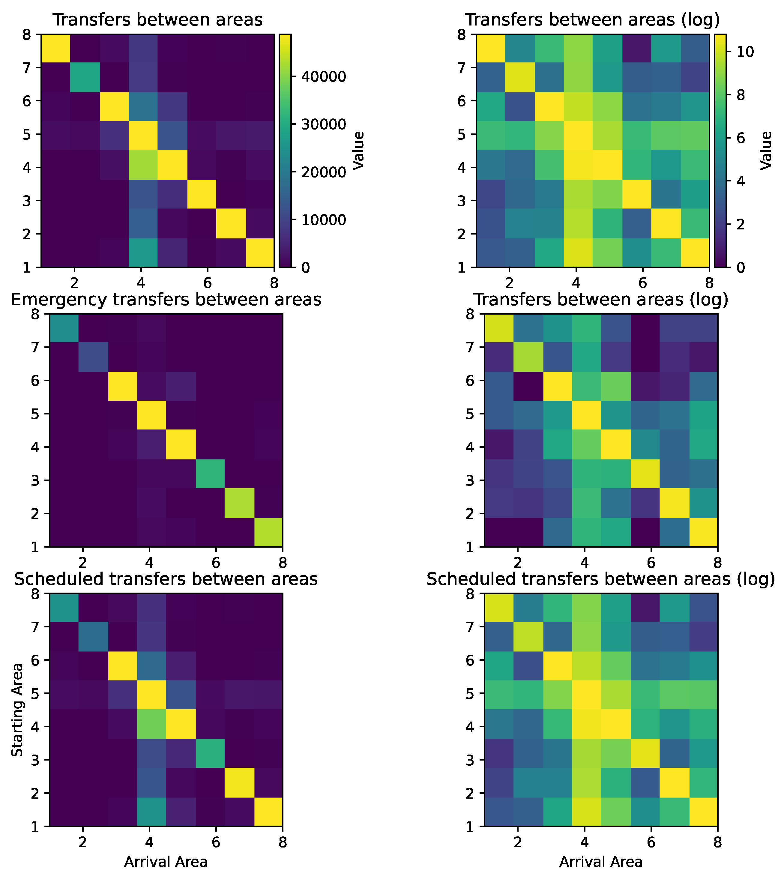
The analysis begins with the visualization of transfers between health areas using heat maps. It can be seen that the number of transfers within the same area is considerably higher compared to those between different areas. In order to highlight the latter, a logarithmic scale is used in the visualization (
Figure 5).
A greater number of transfers is observed in Area IV, especially with regard to programmed services, which is understandable given that this area houses the province’s central hospital. On the other hand, it is observed that, in the case of emergency services, transfers between areas hardly occur, except in those health areas that include large cities (III, IV, and V).
Considering the previous conclusions, where it was indicated that most of the programmed transfers originated in hospitals, an analysis of the destinations of these transfers was carried out. However, it was found that the classification of destinations in the recorded data is indeterminate in most cases, which prevents concrete conclusions from being drawn from this analysis.
4.3.2. Relationship between the Number of Daily Emergencies and the Number of Scheduled Services
As a result of the conclusions obtained, the question arises as to the existence of a possible relationship between the number of daily emergencies and the number of scheduled services. To address this question, a correlation analysis was carried out both in general and for each health area, obtaining values that were always positive, although not very significant. The correlation coefficients are higher in the health areas that include more populated cities. Consequently, there is a weak direct correlation between the number of emergency services and scheduled services. However, the results obtained are not sufficiently conclusive to draw reliable conclusions.
4.3.3. New Time Variables
Other variables that may be determinant in the target prediction are the time variables. However, these variables are very precise and do not provide much information by themselves. Nevertheless, from them, it is possible to derive new variables that continue to provide relevant information. According to the literature analyzed and as will be verified later, variables such as the day of the week, the day of the month, and the day of the year have been identified as important variables in this context. Therefore, an intermediate processing of the data will be performed to obtain the following variables:
From the time of service variable, a new variable corresponding to 6 time slots will be created:
- −
From 00:00 to 04:00;
- −
From 04:00 to 08:00;
- −
From 08:00 to 12:00;
- −
From 12:00 to 16:00;
- −
From 16:00 to 20:00;
- −
From 20:00 to 00:00.
From the date of service variable, new variables will be created that may be more significant, such as:
- −
Day of the week;
- −
Day of the month;
- −
Week of the year;
- −
Month of the year;
- −
Year.
With the new variables, we proceeded to visualize the data and obtain new conclusions. Some of them can be seen in
Figure 6 and
Figure 7. It can be concluded that, in the case of emergency services, the distribution over the days of the week is more or less uniform, although a slight increase is observed on Mondays and a decrease on weekends. However, in the case of scheduled services, there is a marked difference between Saturdays and Sundays compared to the rest of the days.
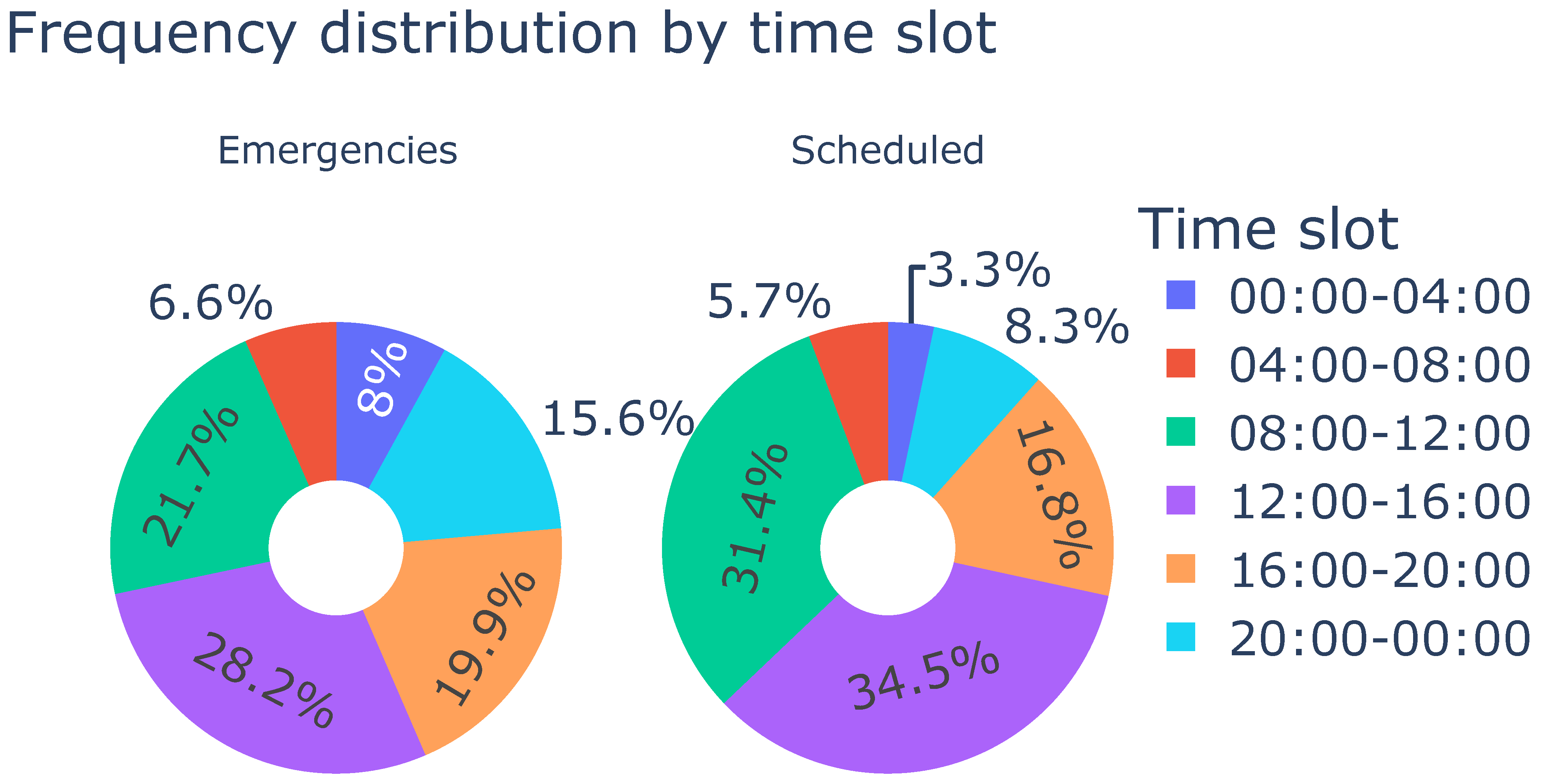
In terms of time slots, for both emergency and scheduled services, a higher concentration of services is observed between 08:00 and 16:00, followed by the afternoon hours. For scheduled services, there is a notable decrease after 20:00, while in the case of emergency services, this decrease does not occur until 00:00.
5. Results
After the exploratory analysis of the data, the data mining techniques explained in
Section 3 were applied. For this, a transactional database is required. Before applying the algorithm, it is necessary to prepare the database by eliminating single or irrelevant variables. In this case, the following considerations are taken into account:
The service time is divided into 6 time slots.
The date variable is eliminated, but new variables related to the day of the week, day of the month, week of the year, month of the year, and year are created.
Taking into account the amount of data available, a support value of was selected, avoiding discarding transactions with a lower frequency that could be relevant. In addition, a confidence value of was set to ensure that the rules generated have an acceptable level of accuracy.
With the selection of these parameters, different combinations of variables such as no escort, stretcher bearer, nurse and/or stretcher were identified, but their presence in the association rules is due to the fact that in more than of the transactions, none of these services are required. Therefore, it is considered that these variables do not provide significant information due to the imbalance in the data, and it is suggested that they should not be taken into account in future analyses.
It can be seen that the origin “Home” is the main one in the scheduled services, something already mentioned above. In addition, there is an evident association between the area and the referral hospital in the area. Another origin, denoted as “collective support”, is always related to scheduled services and is required from home.
Regarding discharges, it is concluded that they are almost always scheduled, also obtaining an association between “Emergencies” and 112 (European Union emergency assistance telephone number) and SAMU (Emergency Medical Care Service—a specialized system that is part of “112” and is specifically dedicated to emergency medical care) calls. Scheduled services tend to be concentrated mainly between 08:00 and 14:00 hours, and a greater number of these are performed from home on Mondays, Wednesdays, and Fridays.
We continued with the Dickey–Fuller test on the objective variable, the number of services, differentiating by health area and whether they are urgent or scheduled services. A significance level of was used. The results indicate that most of the health areas show non-stationarity in scheduled services, except for IV (Oviedo, the capital) and VIII. As for emergency services, non-stationarity cannot be affirmed in most cases, and those that are not stationary have p-values higher than those of the scheduled services.
For those cases in which the Dickey–Fuller test has rejected the null hypothesis and the non-stationarity of the series has been determined, the ACF and PACF were calculated, taking into account up to a difference of 400 days to detect annual, monthly, and weekly stationarity, etc.
In the scheduled services, a weekly seasonality is observed (as shown by the significant autocorrelation at lag 7, 14, and 28 in
Figure 8). This is logical since scheduled services tend to decrease during weekends, which generates a weekly periodicity.
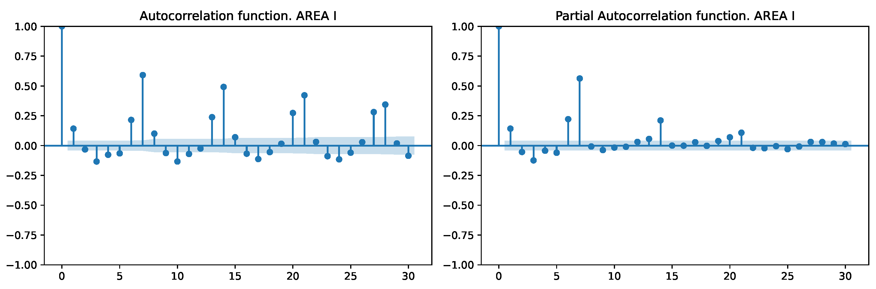
In the health areas where the Dickey–Fuller test identified seasonal patterns, observations in emergency services indicate prominent periods occurring every 1 or 8 days (
Figure 9). This pattern is attributed to the presence of both weekly seasonality and a short-term component at lag 1, with the occurrence at lag 8 arising from the interaction of these factors.
In this case, only variables that can be useful for prediction are considered, so variables such as destination health areas and the need for stretcher-bearers are not taken into account. The variables taken into account are divided into two groups: on the one hand, those obtained directly from the table provided as the starting health area, and on the other hand, those obtained after processing the time of service and date of service variables: day of the week, week of the year, the distinction between emergency and scheduled, day of the month, day of the year, time slot and month of the year.
To compare the effect of taking the stated variables of greatest importance and to be able to make future comparisons, we first started with a predictive model. For this, we used, as a training data set, those services performed between 2016 and 2021 and, as a test sample, the first six months of 2022 since the following ones had incomplete data.
The objective is to evaluate how the use of different predictor variables affects the accuracy of a model according to their correlation with the target variable. As mentioned in
Section 3, the XGB algorithm is used because it allows working with qualitative variables in Python without requiring additional transformations. After the algorithm was fitted with the available data, depending on the indicated metric (weight, gain, or cover), the provided variables were directly displayed and sorted according to their importance.
Taking into account any of the three metrics, the four most important variables, although the order changes depending on the metric, are the same:
It was decided to use the gain metric, which indicates how much the loss function is reduced when dividing a data set according to a specific characteristic.
In situations such as this, where there is a large number of data and variables (even if some have been discarded), determining the importance of predictor variables and observing how models using fewer variables can be equally accurate can significantly reduce the computational cost. The complete order of the variables used is as follows:
In the first instance, the model only considers the time slot, and subsequently, the other variables are added in new models until reaching one that includes all of them. For each model, four metrics are calculated:
Mean squared error (MSE): It is a measure of the average squared difference between the actual and predicted values in a regression model. It quantifies the overall model performance, with lower MSE values indicating a better fit of the model to the data.
Root mean squared error (RMSE): It is the square root of the MSE and represents the standard deviation of the residuals (prediction errors). RMSE is commonly used to interpret the error magnitude in the same units as the target variable.
Coefficient of determination (R-squared, R2): It is a statistical metric that represents the proportion of the variance in the dependent variable (target) that is predictable from the independent variables (features) in a regression model. It ranges from 0 to 1, with higher values indicating a better fit of the model.
Mean absolute error (MAE): It is a metric that measures the average absolute difference between the actual and predicted values in a regression model. Similarly to MSE, it is used to assess the model’s accuracy, but it is less sensitive to outliers since it takes the absolute value of the errors.
Figure 10 shows that using only the four most important variables yields even better results than considering all variables. Halving the number of predictor variables implies a significant reduction in the computational cost associated with the predictions. Having fewer predictor variables to process reduces the complexity of the model and speeds up the execution time, saving both computational resources and CPU and memory time, which is especially useful when handling large data sets or when the model is to be used in real-time applications. Furthermore, with this reduction in variables, the possibility of over-fitting is reduced, and by focusing only on the most important variables, the interpretability of the model is improved.
6. Conclusions
In health transport research, a broad spectrum of data analysis approaches and considerations have been explored. These range from defining clear objectives to selecting the appropriate methods and models for deriving insightful conclusions. Studies specifically targeting spatial and temporal prediction of the number of transport services emphasize the importance of identifying relevant external variables and determining which are critical to the predictions.
Although it was not the main objective of the research, a previous analysis of the correlation and dependence with external variables, as well as the relationship between internal variables, has led to numerous conclusions that can be used not only in the definition of future models but also in current planning.
A study of external variables has been carried out, analyzing their correlation with the number of services. Unique events, such as sports or festive occasions, have been identified to elevate the demand for medical transport services in both emergency and scheduled contexts. This surge in demand is especially evident in less populated areas, where a singular event can amplify the average daily service count by as much as sevenfold. The combination of internal and external variables, along with future research involving other factors such as meteorological conditions, adds greater richness to the data and enables the derivation of new conclusions.
In addition, a strong correlation exists between demographic factors and health transport. In particular, a direct relationship has been found between the overall population and the active population segment with medical transport requirements across various health areas. Both these factors show a high correlation with the number of services, both emergency and scheduled. Interestingly, a significant correlation, close to 0.9, was observed between medical transport and the youth rate, indicating that areas with a higher proportion of young population tend to demand more medical transport services, a finding that might be counterintuitive to some. These results may be useful when determining fleet rates per population since, intuitively, one may think that older people require more health transport services, but this may be more oriented to scheduled services, while younger people require more emergency services.
During the examination of internal variables, significant insights emerged that aid in variable selection. The transfers that occur most frequently between different health areas were identified, along with the most common origins and destinations. Furthermore, specific time slots and weekdays were identified where transfers are more prevalent. Notable seasonality patterns emerged in scheduled services, which were validated through statistical measures such as the Dickey–Fuller test and the analysis of the ACF (autocorrelation function) and PACF (partial autocorrelation function).
The main objective of the study was to identify the determining variables in the prediction of the demand for medical transport. Based on an analysis and review of the literature, eight relevant variables were identified. However, only four of these proved essential for achieving comparable predictive results for service numbers. This reduction in the number of variables not only reduces the computational cost of the prediction models but also improves the interpretability of the results. The four most important variables in the prediction are time slot, health area of departure, day of the week, and the distinction between emergency and scheduled.
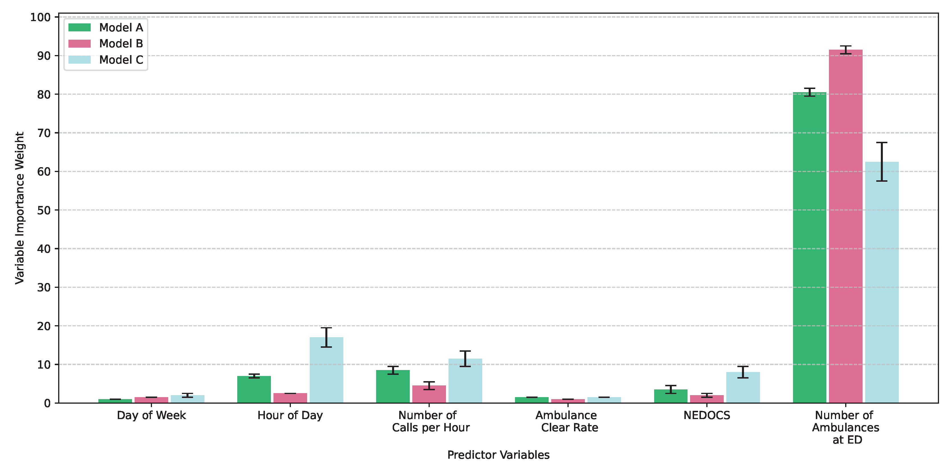
In this case, the amount of fleet (which was the most important factor in
Figure 1) was not of interest since it is something that can be determined when the prediction based on it is known. This research has made it possible, on the one hand, to counter previous research with a new data set and, on the other hand, to determine that the gradient boosting algorithm yields similar results to previous ones. In addition, as a novelty, an analysis of the variation in the metrics has been carried out as the number of variables used increases.
Several promising lines of future research have emerged from this study. Firstly, exploring different predictive models and their respective hyperparameters is a logical next step. Using a comparative benchmarking approach, balancing computational expense with model interpretability, can help identify the best strategies. Additionally, exploring real-time data integration could further enhance prediction accuracy.


 ,
, 


