Abstract
The number of loan requests is rapidly growing worldwide representing a multi-billion-dollar business in the credit approval industry. Large data volumes extracted from the banking transactions that represent customers’ behavior are available, but processing loan applications is a complex and time-consuming task for banking institutions. In 2022, over 20 million Americans had open loans, totaling USD 178 billion in debt, although over 20% of loan applications were rejected. Numerous statistical methods have been deployed to estimate loan risks opening the field to estimate whether machine learning techniques can better predict the potential risks. To study the machine learning paradigm in this sector, the mental health dataset and loan approval dataset presenting survey results from 1991 individuals are used as inputs to experiment with the credit risk prediction ability of the chosen machine learning algorithms. Giving a comprehensive comparative analysis, this paper shows how the chosen machine learning algorithms can distinguish between normal and risky loan customers who might never pay their debts back. The results from the tested algorithms show that XGBoost achieves the highest accuracy of 84% in the first dataset, surpassing gradient boost (83%) and KNN (83%). In the second dataset, random forest achieved the highest accuracy of 85%, followed by decision tree and KNN with 83%. Alongside accuracy, the precision, recall, and overall performance of the algorithms were tested and a confusion matrix analysis was performed producing numerical results that emphasized the superior performance of XGBoost and random forest in the classification tasks in the first dataset, and XGBoost and decision tree in the second dataset. Researchers and practitioners can rely on these findings to form their model selection process and enhance the accuracy and precision of their classification models.
1. Introduction
Conventional methods of credit risk assessment to approximate the likelihood of potential losses rely mainly on credit scores and reports. Such reports usually do not provide comprehensive information about the borrower’s creditworthiness since multiple factors, like financial indicators, demographic data, and customer behavior, like transactions and spending history, also play a significant role in credit risk assessments. To handle such a large number of factors and provide more comprehensive and large-scale assessments, supervised machine learning algorithms can be used. The study conducted by Singh Saini, Bhatnagar, and Rani in 2023 illustrates that the Random Forest Classifier exhibited the highest accuracy at 98.04%, surpassing the K-Nearest Neighbors Classifier (78.49%) and Logistic Regression (79.60%). These findings underscore the significant potential of machine learning algorithms, as highlighted in their research, to enhance the loan approval process and diminish the risk of loan defaults [1].
Only in America, more than 20 million Americans were burdened with open loans in 2022 accumulating a total debt of USD 178 billion, although over 20% of loan applications were met with rejection. Such situations lead to missed opportunities for both parties involved. A bank’s profit or loss depends mostly on loans i.e., whether the customers are paying back the loan or defaulting. By predicting the loan defaulters, the bank can reduce its Non-Performing Assets [2]. Loan candidates differ by a large number of factors ranging from financial habits to demographics. Machine learning algorithms can be used as a significant tool to incorporate additional factors to identify potential risks and suitable loan candidates, making the process of decision making for banking industries easier and more reliable [3,4].
Various cultures notably influence financial habits, which makes demographics an important factor in loan management. Hence, different countries usually need unique approaches for credit management. In 2008 in Spain, for instance, the high level of exposure to the real estate market and substantial borrowing needs placed the sector in a position of vulnerability to a deterioration in economic activity in Spain and borrowing conditions on international capital markets. The period from 2007 to 2011 was therefore characterized by a rapid slowdown in lending up to mid-2009, followed by a drop that subsequently accentuated, going from annual growth of over 17% in 2007 to a drop of 3.8% in 2011. In turn, there was a sharp rise in bad loans, particularly loans to the real estate and construction sector, in a context of worsening financial conditions for real estate businesses, whose situation progressively deteriorated, given the impossibility of freeing themselves from their financial burdens by liquidating their real estate assets [5]. The research shows that, in the UK, people from ethnic minorities are more likely to be denied loans, even those having good income and credit scores [6].
On the other hand, financial behavior is generally affected by mental health conditions. Reports show that 56% of those with mental health problems experienced financial hardship when managing their credit, compared with only 28% of those without mental health problems [7].
The primary motivation for this research stems from the increasing importance of assessing borrowers’ creditworthiness in the modern financial landscape.
The goal of this study is to investigate whether machine learning algorithms can enhance the credit risk prediction process, ultimately benefiting both financial institutions and borrowers. To achieve this objective, experiments using a mental health dataset and a loan approval dataset are conducted. Specifically, this paper aims to:
- Propose an intelligent credit risk prediction system that integrates mental health data into supervised machine learning algorithms;
- Conduct a comprehensive evaluation of multiple classification techniques to identify the optimal methodology that minimizes overfitting and maximizes performance in credit risk predictions;
- Analyze the key factors that influence loan approvals and explore their interdependencies with the response variable, and;
- Establish a framework for future research endeavors that can enhance the accuracy of predictive models, while also shedding light on the ethical considerations associated with the utilization of mental health data.
By addressing these objectives, this study contributes to the ongoing efforts to improve credit risk assessment and lending practices, aiming to provide more accurate assessments and reduce the potential financial burden on both borrowers and lending institutions.
This paper is meticulously structured to guide readers through a logical progression of the research. It commences with Section 1, where the context, motivations, objectives, and contributions of the study are presented. Following the introduction, Section 3 offers a detailed description of the two datasets used in this research—the mental health dataset and the loan approval dataset—highlighting their relevance to the study. Section 4, introduces the selected machine learning algorithms and explains the reasons for choosing them, thereby laying the foundation for the subsequent analytical components. Section 5 outlines the steps involved in the data acquisition, analysis, and model evaluation, offering valuable insights into the research process. Progressing to Section 6, a comprehensive analysis of the outcomes for both datasets is presented, providing an in-depth examination of the findings. Both Section 2 and Section 7 conduct a thorough comparison with prior studies on similar topics, providing a crucial research context. Section 8 succinctly summarizes the findings, contributions, and implications of this study, offering a comprehensive overview of its significance. This well-organized and structured approach ensures that readers can seamlessly navigate the paper, gaining a comprehensive understanding of the research presented.
2. Related Research
In their 2023 study, Bhargav and Sashirekha introduced a novel approach by leveraging random forest classifiers to evaluate diverse machine learning methods for forecasting loan approvals. Drawing from Kaggle’s repository, they employed loan prediction datasets to scrutinize accuracy and loss metrics. The random forest method presented a precision of 79.44% and a loss of 21.03%, surpassing the conventional decision tree algorithm, which yielded a precision of 67.28% and a loss of 32.71% in a sample of 20 instances. The subsequent statistical examination via an independent sample t-test resulted in a p-value of 0.33, indicating no noteworthy differences between the techniques at a 95% confidence level. This investigation suggests that random forest emerges as a more adept predictor of loan approval compared to the decision tree model [8].
Wang and colleagues (2023) [9] devised a novel stacking-based model aimed at evaluating the risks in financial institutions, determining the most effective model through performance comparisons. Their work extended to crafting a bank approval model using deep learning on imbalanced data, employing a convolutional neural network for feature extraction, and implementing counterfactual augmentation for achieving balanced sampling results. The fine-tuning of the auto finance prediction model, grounded in bank model features, resulted in a substantial 6% boost in the joint loan approval, as substantiated by the experiments conducted on real-world data.
Abdullah and colleagues (2023) [10] explored a range of machine learning techniques to forecast nonperforming loans within financial institutions in emerging countries. By examining the data from 322 banks spanning 15 nations, their comprehensive analysis revealed that advanced machine learning models, particularly random forest, surpassed linear methods, achieving an accuracy of 76.10%. Notably, bank diversification surfaced as the pivotal predictor, surpassing macroeconomic factors in the prediction of nonperforming loans.
In their 2020 study, Alsaleem and Hasoon examined the performance of machine learning algorithms in the assessment of bank loan risks, focusing on conventional methods with the aim of achieving higher accuracy. Notably, they observed that multilayer perceptron (MLP) outperformed the random forest, naive Bayes (NB), and DTJ48 algorithms in categorizing bank loan risks. The evaluation of the model’s performance was conducted using traditional metrics on a dataset comprising 1000 loans and their corresponding repayment status [11].
In Section 7, additional research papers are analyzed and discussed, focusing on their contributions and shortcomings that are resolved within the scope of this research.
3. Input Datasets: Mental Health and Loan Approval
According to the World Health Organization, about one in four people worldwide has a mental illness [12]. These struggles largely impact the economic decision making and behavior of the individuals. As a consequence, individuals struggling with mental health issues can find it challenging to maintain steady employment or earn a stable income, making it difficult for them to meet their financial obligations and be approved to obtain loans.
Lenders evaluate various factors, such as credit score, income, and the debt-to-income ratio, to determine the borrower’s ability to repay the loan. Mental health is also one of the crucial factors that can significantly impact a person’s financial situation.
Mental health problems, such as depression, post-traumatic disorder, anxiety, and others, can lead to periods of instability, resulting in missed payments, affecting a person’s decision-making ability, leading to impulsive spending or poor financial choices, or even bankruptcy. If an applicant has a history of mental health conditions or presents signs of instability, a lender can perceive him or her as a higher-risk borrower, leading to either a denial of the loan application or stricter loan terms, such as higher interest rates or collateral requirements.
The research shows that mental health issues in the workplace can lead to increased absenteeism, reduced productivity, and decreased employee engagement. Around 70% of adults in the USA are employed with depression resulting in an estimated 35 million missed work days annually and costing employers USD 105 billion due to reduced productivity. To mitigate this problem, Mental Health First Aid should be introduced to improve mental health literacy among employees. It is the responsibility of employers to provide comprehensive benefits packages that support mental health and flexible working arrangements [13,14,15].
However, it is essential to note that mental health should not be a barrier to accessing loans or financial resources. Instead, financial institutions should adopt inclusive policies and practices that recognize the diverse needs of borrowers, including those with mental health conditions. This can include providing tailored financial education and counseling services, flexible loan terms, or partnering with mental health professionals to support borrowers in managing their finances.
3.1. Mental Health Dataset
The first dataset that was used as one of the two input variables for the prediction models in this paper was ‘Mental Health at Workplace’, containing survey responses from 1991 individuals who worked in various industries across the United States. The survey was conducted to collect data on employees’ attitudes toward mental health and their experiences with mental health issues in the workplace. The dataset included data with 1991 instances and 25 attributes, as shown in Table 1.

Table 1.
Mental health dataset (input variables).
3.2. Loan Approval Dataset
The second input dataset consisted of various properties that could significantly impact loan approval. By analyzing these data, the most crucial factors that influenced loan approvals could be identified and used by robust machine learning models to accurately predict the likelihood of a loan approval.
One of the significant factors for loan approvals is a good credit history, which highlights the importance of maintaining a good credit score and paying bills on time. Also, lenders tend to favor individuals with higher income levels to borrow higher loans as they are considered more capable of making repayments. The loan amount and loan terms are also critical factors for determining loan approval. Smaller loans with shorter repayment terms generally have a higher chance of approval, as they are perceived as less risky for lenders. Another factor is the location as urban properties tend to have higher approval rates than rural properties. A not-so-obvious factor is the education level that can also influence the loan approval. Individuals with higher education levels tend to have better financial stability and a better ability to repay loans since education level is seen as a proxy for financial literacy and responsibility.
By understanding these factors and their impacts on loan approval outcomes, lenders can make more informed decisions when considering loan applications. Such factors are shown in Table 2.
Table 2.
Loan approval dataset (input variables).
The output variable, as seen in Table 3, is a crucial component of the analysis, as it signifies the loan approval status, which can be categorized as two distinct outcomes: ‘approved’ (Yes) or ‘not approved’ (No). These designations hold substantial implications for the individuals seeking financial assistance and for our overall assessment of the lending process.
Table 3.
Loan approval dataset (output variables).
Delving deeper into the data, a noteworthy distribution within this output variable was encountered. The examination revealed that there were approximately 40,000 instances where loans were not approved (No), signifying a substantial portion of loan applications that did not meet the necessary criteria for approval. This was a critical statistic that prompted further investigations into the factors contributing to these disapprovals.
Conversely, there were approximately 30,996 instances of loans that were approved (Yes), suggesting a substantial number of successful loan applications. These data points are equally important, as they indicate the effectiveness of the loan approval process in facilitating financial support for those in need.
Understanding the balance between these two categories—false (No) and true (Yes)—was pivotal for the analysis. It allowed us to assess the overall performance of the loan approval system, identify areas for improvement, and ultimately enhance the financial well-being of our clients.
4. Machine Learning Algorithms to Use for Loan Predictions
Loan prediction is a crucial task in the financial industry. By leveraging historical loan data and various features, machine learning algorithms can learn patterns and predict whether a loan application should be approved or rejected. By employing this diverse set of machine learning algorithms, comprehensive insights into loan predictions can be obtained, considering various perspectives and leveraging the strengths of each algorithm.
4.1. Decision Tree
A decision tree is a tree-like model created by recursively splitting the dataset into smaller subsets. These subsets are based on the feature that provides the most information obtained for the task at hand. Internal nodes represent a decision based on a feature, and the leaf nodes are assigned to classes representing the most appropriate target value. The leaf can hold a probability vector indicating the probability of the target attribute having a certain value.
Decision trees are particularly useful in situations, like credit risk predictions, where the relationship between the input features and the output variable is nonlinear and complex [16]. Decision trees are also preferable due to their structure that can be easily visualized and understood, which is useful for explaining the decision-making process to stakeholders. Decision trees can also be used in combination with other machine learning techniques, such as ensemble methods, to improve their performance and robustness.
Naturally, decision makers prefer less complex decision trees since they can be considered more comprehensible. Some research suggests the tree’s complexity has a crucial effect on its accuracy [17]. Usually, the tree’s complexity is measured by one of the following metrics: the total number of nodes, the total number of leaves, the tree depth, and the number of attributes used.
4.2. Random Forest
Random forest is an ensemble learning algorithm combining multiple decision trees, where each tree is built on a random subset of the features and training data to make a prediction. Particularly in the case of this study, the randomness helped to reduce the correlation between the trees, and the final prediction of the model was obtained by averaging the predictions of all the trees. Also, random forest can handle large datasets with a large number of features, handles missing and noisy data, and is robust to outliers. Recent research has focused on improving the performance of random forest by optimizing the hyperparameters and feature selection techniques. For example, some studies used genetic algorithms to optimize the hyperparameters of the model [18], while others used permutation feature importance to identify the most important features and exclude the less relevant ones [19].
4.3. Naive Bayes
Naive Bayes [20] is a classification algorithm widely used in machine learning to classify data into different classes based on their properties. The algorithm is based on Bayes’ theorem, which describes the probability of an event occurring given the prior knowledge of the conditions that might be associated with the event. In a naive Bayes classifier, the probability that a data point belongs to a particular class is estimated based on the probabilities of each feature in that class. The term ‘naive’ is used because this estimation is performed for each feature separately.
This algorithm is chosen for this research since, despite its simplicity, naive Bayes has proven its prowess in various classification tasks, especially natural language processing and text classification, and is found to be effective in classifying large-scale datasets with a high accuracy, including spam email filtering and sentiment analysis.
4.4. KNN
The K-nearest neighbors (KNN) algorithm [21] is a classification algorithm used in fields like image recognition, speech recognition, and natural language processing. Its basic concept is to determine the class of a new data point based on the classes of its K-nearest neighbors in the training dataset. The reason for predictions using the k-nearest neighbors method is based on the assumption that objects of neighbors have similar prediction values. In other words, KNN measures the distance between a new data point and each point in the training dataset making it a distance-based measuring approach using methods, like Euclidean, Manhattan, and Chebyshev distances.
There are modifications to the algorithm, like KNN-SI (KNN with sparse interactions), which proposes using sparse matrices to represent pairwise interactions between features in a dataset bottom, reducing the computational complexity and enhancing the accuracy of the KNN algorithm [22]. Another modification of the KNN algorithm can be the weighted KNN, which improves the accuracy of the algorithm by giving more weight to the closest neighbors [23].
4.5. Boosting Algorithms
Boosting is a family of machine learning algorithms that combine a set of weak learners to create a stronger and more accurate prediction model. A ‘weak learner’ is a model that performs only slightly better than random guessing. The idea behind boosting algorithms is to iteratively train a sequence of weak learner models on the same dataset, after which the predictions of all of them are combined to obtain the final prediction. Such an approach aims to progressively improve the accuracy of the model through iterations. Misclassified examples in each iteration are assigned higher weights in the subsequent iteration, ensuring that the subsequent weak learner focuses on the most difficult examples that the previous learner failed to classify correctly.
4.5.1. AdaBoost
Adaptive boosting or AdaBoost is a popular binary classification algorithm that is used in the training set, meaning that various weights are assigned to each training example and the predictions of multiple weak learners are combined to obtain the final prediction. AdaBoost can adapt to the complexity of the data, which was ideal for the case of this study, and handle noisy or imbalanced datasets. In each iteration, the algorithm assigns higher weights to misclassified examples, allowing it to focus on the most difficult examples and learn from its own mistakes. AdaBoost can also work with weak learners, like decision trees, neural networks, and support vector machines.
However, when AdaBoost becomes too complex and memorizes the training data, it becomes more susceptible to overfitting, which can be prevented by limiting the number of iterations. Adaptive boosting with differentiable loss functions (AdaBoostDL) is among the several extensions of AdaBoost that use the loss function to train weak learners. In such a way, the non-differentiable data are handled and the stability of the algorithm can be improved [24,25].
4.5.2. Gradient Boosting
Similar to AdaBoost, gradient Boosting is a binary classification algorithm that combines the predictions of multiple weak learners. However, unlike AdaBoost, which focuses on the misclassified examples in each iteration, gradient boosting uses the gradient descent to minimize a loss function iteratively. Gradient boosting handles a wide range of loss functions to automatically detect and model non-linear relationships between the features and target variable [26,27].
4.5.3. XGBoost
Extreme gradient boosting (XGBoost) is introduced as an extension of gradient boosting that uses a combination of gradient descent and second-order Taylor expansion to improve the accuracy and speed of the algorithm. The algorithm starts with an initial model and then adds new models to the ensemble iteratively, to upgrade the performance of the current ensemble. The new models are trained to predict the negative gradients of the loss function concerning the current predictions.
One of the key innovations of XGBoost is the use of the second-order Taylor expansion to approximate the loss function. This allows XGBoost to model the curvature of the loss function and improve the accuracy of the predictions. Additionally, XGBoost includes several regularization techniques and can handle missing values and sparse data without the need for preprocessing. It also supports parallel processing and can be run on distributed systems, which makes it suitable for large-scale machine-learning tasks [25,28].
In recent years, several improvements and extensions of XGBoost have been proposed. For example, LightGBM, introduced by Ke et al. in 2017 [29], is a similar algorithm that uses a different approach to handling the gradient and Hessian matrices. LightGBM is designed to be even faster and more memory efficient than XGBoost, and has achieved a state-of-the-art performance for several benchmark datasets.
The process of selecting machine learning algorithms for this study involved a rigorous evaluation of their technical characteristics and suitability for the credit risk prediction task. The criteria for algorithm selection encompassed considerations, such as their performance in prior credit risk analysis studies, ability to handle diverse and high-dimensional datasets, and relevance to the financial domain.
Two gradient boosting algorithms, XGBoost and GradientBoost, were chosen for their exceptional robustness in determining complex relationships in the datasets. Their ensemble-based methodology allowed for sequential improvements in the predictive accuracy, making them adept at discerning intricate patterns in the credit-related data.
K-nearest neighbors (KNN) was included due to its effectiveness in capturing patterns based on proximity, particularly in scenarios where spatial correlations among data points were significant. Its non-parametric nature makes it especially useful when the underlying distribution of the data is not explicitly known.
For versatility in handling both categorical and numerical features, we incorporated both random forest and decision tree algorithms into our ensemble. The former enhanced the predictive accuracy and robustness against overfitting.
The simplicity and efficiency of naive Bayes made it a valuable addition to our ensemble. It operated well under the assumption of feature independence, offering a probabilistic classification approach that complemented the other models.
AdaBoost was chosen for its ability to adapt to the weaknesses of individual models. Through iterative training, AdaBoost enhanced the predictive performance and contributed to the ensemble’s overall resilience.
The rationale behind assembling this diverse set of algorithms lies in harnessing their complementary strengths and characteristics. This approach aims to synergize the predictive capabilities of the ensemble, ensuring a comprehensive exploration of the credit risk prediction landscape. The detailed technical criteria considered during the algorithm selection contribute to the methodological rigor of this study, providing a foundation for robust and insightful analyses.
5. Methodology
This section presents a detailed description of the methodology used to obtain the results for the loan approval prediction. The code snippet implemented in Python version 3.11.0 included various steps, including data preprocessing, model selection, training, evaluation, and visualization. Each step is explained in the subsequent text, highlighting the reasoning behind the selected choices and techniques.
5.1. Importing Libraries and Datasets
Several libraries that play a crucial role in data manipulation, machine learning, and visualization were imported, including Pandas (version 1.5.3) for the data manipulation and analysis, providing data structures, such as DataFrames, which allowed the efficient handling of structured data; NumPy (version 1.24.2) for numerical computations, enabling efficient array operations and mathematical functions; scikit-learn (version 1.2.2) for model training, evaluation, and preprocessing purposes; matplotlib (version 3.7.1) that enabled the creation of plots, charts, and figures; and seaborn (version 0.12.2), which was a statistical data visualization library built on top of matplotlib, providing additional high-level functions for creating attractive and informative visualizations.
Furthermore, the dataset was sourced from a GitHub repository and loaded into a Pandas DataFrame. The dataset served as the basis for the loan approval prediction research in this paper.
5.2. Data Preprocessing
To prepare the dataset for modeling, a series of preprocessing steps were undertaken. In this research, label encoding as a preprocessing technique of converting categorical variables into numerical representations that could be understood by machine learning algorithms was employed.
The dataset initially presented a diverse array of gender values, reflecting the rich tapestry of human identities and expressions. Among the recorded gender labels were ‘Female’, ‘M’, ‘Male’, ‘male’, ‘female’, ‘m’, ‘Male-ish’, ‘maile’, ‘Trans-female’, ‘Cis Female’, ‘F’, ‘something kinda male?’, ‘Cis Male’, ‘Woman’, ‘f’, ‘Mal’, ‘Male (CIS)’, ‘queer/she/they’, ‘non-binary’, ‘Femake’, ‘woman’, ‘Make’, ‘Nah’, ‘All’, ‘Enby’, ‘fluid’, ‘Genderqueer’, ‘Female’, ‘Androgyne’, ‘Agender’, ‘cis-female/femme’, ‘Guy (-ish) ^_^’, ‘male leaning androgynous’, ‘Male’, ‘Man’, ‘Trans woman’, ‘msle’, ‘Neuter’, ‘Female (trans)’, ‘queer’, ‘Female (cis)’, ‘Mail’, ‘cis male’, ‘A little about you’, ‘Malr’, ‘p’, and ‘femail’, as well as ‘Cis Man’ and ‘ostensibly male, unsure what that really means’.
Recognizing the need for consistency and simplicity in our dataset, the data preprocessing started by implementing a function called change_gender(y) that intelligently transformed the diverse array of gender labels into a more manageable set of categories. This function achieved the following mapping:
If the gender label was any variation of ‘Male’ (e.g., ‘Male’, ‘M’, ‘male’, ‘m’, ‘maile’, ‘Mal’, ‘Mail’, ‘Man’), it was uniformly recoded as ‘M’ to represent the male gender.
Similarly, if the gender label was any variation of ‘Female’ (e.g., ‘Female’, ‘female’, ‘f’, ‘F’, ‘femail’), it was homogenized as ‘F’ to signify the female gender.
All other gender labels that did not fall into the ‘Male’ or ‘Female’ categories were grouped under ‘Other’, providing a broader classification that respected diverse gender identities and expressions.
This meticulous preprocessing step resulted in a dataset that was more manageable and interpretable, with a clear distinction between male, female, and other gender categories. This transformation streamlined the analysis and ensured that gender-related insights were derived from a more coherent and representative dataset, ultimately enhancing the quality of the research and decision-making processes.
Before applying label encoding, it was crucial to handle missing values in the dataset since they could introduce bias and affect the performance of the machine learning models. Hence, a comprehensive missing values check was performed and appropriate strategies to handle missing values were applied. Firstly, missing values in the dataset were checked using the following code snippet:
| missing_values = df.isnull().sum() |
By applying the isnull() method to the DataFrame(df) and then summing the resulting Boolean values, the count of missing values for each column was obtained. This allowed us to identify the features that had missing values and assess the extent of missingness in the dataset.
Once the missing values were identified, we needed to proceed with handling them. Depending on the specific characteristics of the dataset and the nature of the missing values, different strategies could be employed. In this research, the following approach was adopted:
Numeric Features: for numeric features with missing values, the missing values were replaced with the mean value of the respective column, assuming that the missing values were missing at random and that the mean value was a suitable estimate:
| numeric_features = [‘numeric_attribute_1’, ‘numeric_attribute_2’] for feature in numeric_features: df[feature].fillna(df[feature].mean(), inplace = True) |
Categorical Features: for categorical features with missing values, the missing values were replaced with the most frequent category (mode) of the respective column assuming that the missing values could be imputed to the most common category:
| categorical_features = [‘categorical_attribute_1’, ‘categorical_attribute_2’] for feature in categorical_features: df[feature].fillna(df[feature].mode()[0], inplace = True) |
By employing these strategies, we ensured that the missing values for both the numeric and categorical features were appropriately handled, maintaining the integrity of the dataset.
After handling the missing values, the label encoding technique was used. The encoded features were then used as inputs to train the machine-learning models.
To enhance the effectiveness of the data analysis and machine learning models, the one-hot encoding technique was used, which was particularly valuable when dealing with categorical variables, as it helped to convert them into a numerical format that could be comprehended by machine learning algorithms.
In the dataset preprocessing stage of this research, the focus was on the ‘Age’ variable and a set of categorical columns. The goal was to transform these categorical columns into a structured format that could be seamlessly integrated into the analytical workflow.
| dfX = pd.concat([dataset[“Age”],pd.get_dummies(dataset[categorical_columns])], axis = 1) dfY = dataset[“obs_consequence”] dfX |
In the first dataset, categorical columns, such as ‘Gender’, ‘Country’, ‘self_employed’, ‘family_history’, ‘treatment’, ‘work_interfere’, ‘no_employees’, ‘remote_work’, ‘tech_company’, ‘benefits’, ‘care_options’, ‘wellness_program’, ‘seek_help’, ‘anonymity’, ‘leave’, ‘mental_health_consequence’, ‘phys_health_consequence’, ‘coworkers’, ‘supervisor’, ‘mental_health_interview’, and ‘phys_health_interview’ were created. Additionally, there was a column called ‘mental_vs_physical.’
In the second dataset, the categorical columns were ‘Married/Single’, ‘House_Ownership’, ‘Car_Ownership’, ‘Profession’, and ‘City’. These columns provided categorical information about individuals in this dataset.
The process was begun by isolating the ‘Age’ column, as well as the categorical columns that required encoding. These categorical columns contained valuable information, but needed to be converted for machine-learning compatibility.
With the ‘Age’ column and the one-hot encoded representations of the categorical columns prepared, the pd.concat function was used to combine these DataFrames horizontally (along the columns axis). This resulted in a new data frame named dfX.
The power of one-hot encoding was represented by the pd.get_dummies function. This function efficiently transformed the categorical columns into binary columns, where each unique category became a new binary column. If a row belonged to a particular category, the corresponding binary column received a value of 1; otherwise, it received a value of 0.
The resulting dfX DataFrame presented a mixture of numerical and binary columns at this stage, where the binary columns represented the various categories present in the original categorical columns. This transformation enabled us to effectively include these categorical variables in the machine learning models.
As a final step, the target variable ‘obs_consequence’, was also prepared and stored in a separate data frame named dfY. This separation of predictors (dfXs) and target variables (dfYs) adhered to the best practices for machine learning.
In the provided code snippet, the preprocessing LabelEncoder() function from scikit-learn was utilized to perform label encoding. The categorical features that needed to be encoded in the encoded_features list were specified. By iterating over these features, the label encoding transformation of each feature in the dataset could be applied.
The code snippet below demonstrates the application of label encoding to the categorical features in the dataset:
| abel_encoder = preprocessing.LabelEncoder() encoded_features = [‘attribute_1’, ‘attribute_2’, ‘attribute_3’, ‘attribute_4’] for feature in encoded_features: df[feature] = label_encoder.fit_transform(df[feature]) |
5.3. Model Selection
After the data preprocessing stage, the subsequent critical step was selecting an appropriate machine learning algorithm for the loan approval prediction. The K-nearest neighbors (KNN) classifier was considered as the primary model in this study. The KNN algorithm is a non-parametric method that classifies an unlabeled data point based on the class labels of its k-nearest neighbors in the feature space. Alternative algorithms in the code were also explored to enable the experimentation and comparison of their performances. These algorithms included Gaussian naive Bayes (GNB), random forest classifier (RFC), decision tree classifier (DTC), AdaBoost classifier (ABC), gradient boosting classifier (GBC), and XGBoost classifier (XGBC). Each algorithm had its strengths and weaknesses, and selecting the most appropriate one depended on the specific requirements of the loan approval prediction task. By including multiple algorithms, their comparative performances could be assessed and the most suitable one could be chosen based on the evaluation metrics and domain knowledge.
5.4. Train–Test Split
During the train–test split process, various corner cases that could arise and impact the model evaluation were considered. The corner cases included handling imbalanced datasets, stratified sampling, and setting a random seed for reproducibility.
In real-world scenarios, datasets often exhibit a class imbalance, where one class is more prevalent than another. A random split during the train–test split can result in an imbalanced distribution of classes in the training and testing sets. Stratified sampling can be employed as one of the techniques to ensure that the class distribution is maintained in both the training and testing sets, providing a more representative evaluation and more accurate results. The train_test_split function in scikit-learn supported stratified sampling by specifying the ‘stratify’ parameter as the target variable (‘y’):
| X_train, X_test, y_train, y_test = train_test_split(X, y, test_size = 0.2, stratify = y) |
Stratified sampling is also crucial when working with small datasets or datasets where certain classes are underrepresented. By maintaining the class distribution during the train–test split, each class was adequately represented in both sets, enabling the model to learn from and evaluate diverse instances.
As seen in Figure 1, since the loan approval dataset has a relatively balanced distribution between the two classes (approved and not approved), the need for stratification is reduced.
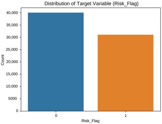
Figure 1.
Distribution of target variables.
Stratification is more crucial when dealing with highly imbalanced datasets, where one class significantly outnumbers the other. In such cases, it helps ensure that both classes are represented adequately in the training and testing sets.
To ensure the reproducibility of the experiments, it was essential to set a random seed when performing the train–test split. This allowed us to obtain the same split each time the code was run, facilitating a consistent evaluation and comparison of the models.
| X_train, X_test, y_train, y_test = train_test_split(X, y, test_size = 0.2, random_state = 42) |
By setting the ‘random_state’ parameter to a specific value (e.g., 42), it was ensured that the train–test split was deterministic, yielding the same split every time the code was used.
Taking into account these corner cases enhanced the robustness and reliability of the model evaluation. It ensured that the model was evaluated for the representative data, considered class imbalance, and allowed for the reproducibility of the experimental results.
5.5. Model Training
The chosen machine learning model was trained using the fit method, which was a fundamental function in scikit-learn that allowed the model to learn from the provided training data. The training data, consisting of the encoded features (X_train) and the corresponding risk flag labels (y_train), were provided as inputs for the fit method for each machine learning algorithm in this research:
| model.fit(X_train, y_train) |
5.6. Model Evaluation
To evaluate the models’ performances after training, various evaluation metrics to assess their predictive capabilities were used. The evaluation metrics provided insights into the models’ accuracy, precision, recall, and F1 score (all described in Section 6: Results), providing a comprehensive understanding of their performance outcomes. During the model evaluation stage, the prediction method of the trained model was used to generate predictions (y_pred) for the testing set (X_test). These predictions were compared to the true labels (y_test) to calculate the evaluation metrics.
| y_pred = model.predict(X_test) accuracy = accuracy_score(y_test, y_pred) f1 = f1_score(y_test, y_pred) precision = precision_score(y_test, y_pred) recall = recall_score(y_test, y_pred) confusion_mat = confusion_matrix(y_test, y_pred) |
5.7. Confusion Matrix and Visualization
In the previous step, in addition to the evaluation metrics, the code also computed the confusion matrix using the confusion_matrix function from scikit-learn, providing a tabular representation of the model’s predictions against the actual labels. It allowed for the analysis of true negatives (TNs), false positives (FPs), false negatives (FNs), and true positives (TPs), thereby enabling a more comprehensive understanding of the model’s performance.
To enhance the interpretability of the confusion matrix, the seaborn library was imported to create a heatmap visualization. The heatmap displayed the confusion matrix with annotations for each category, offering a visual representation of the model’s predictive accuracy and potential misclassifications.
| labels = [‘Negative prediction’, ‘Affirmative prediction’] confusion_mat = confusion_matrix(y_test, y_pred, labels = labels) fig, ax = plt.subplots(figsize = (8, 6)) sns.heatmap(confusion_mat, annot = True, fmt = ‘d’, cmap = ‘Blues’, xticklabels = labels, yticklabels = labels, ax = ax) ax.set_xlabel(‘Predicted’) ax.set_ylabel(‘True’) |
In the code, a subplot with a specified figure size was created to accommodate the heatmap. The sns.heatmap function was used to generate the heatmap, with the following parameters:
- confusion_mat: the confusion matrix to be visualized.
- annot = True: enabled the annotation of each cell in the heatmap with the corresponding count.
- fmt = ‘d’: formatted the annotations as integers.
- cmap = ‘Blues’: specified the color map for the heatmap.
- xticklabels = labels: set the labels for the x-axis tick marks to the specified labels.
- yticklabels = labels: set the labels for the y-axis tick marks to the specified labels.
- ax = ax: specified the subplot to which the heatmap was plotted.
The resulting heatmap provided a clear and concise visualization of the confusion matrix, allowing us to observe the distribution of correct and incorrect predictions across different categories. By examining the heatmap, the patterns and potential areas of improvement in the model’s performance could be identified.
6. Results
The results obtained from the model evaluation, including the accuracy, F1 score, precision, recall, and the confusion matrix, are printed by the console providing valuable insights into the effectiveness of the chosen machine learning algorithm for the loan approval prediction.
The base metric used for model evaluations is often accuracy, describing the number of correct predictions over all the predictions:
The subsequent metric is precision, which measures how many of the positive predictions made are correct (true positives):
Recall is a measure of how many of the positive cases the classifier correctly predictes, over all the positive cases in the data:
The F1 score is a measure combining both precision and recall. It is generally described as the harmonic mean of the two:
The confusion matrix visualization allowed for a comprehensive analysis of the model’s classification accuracy and error rates. The practical realization of the algorithms was carried out in the Python programming language, with several established libraries, such as Pandas, Numpy, and Sklearn, being utilized for data processing. Upon loading the dataset, preprocessing was performed to enhance the algorithm’s efficacy, leading to more favorable results.
6.1. The Evaluation of the First Dataset: Mental Health
The model was trained on a training dataset, with a ratio of 80:20 for the training and test data. Table 4 shows the resulting metrics after implementing the chosen algorithms in the study.
Table 4.
Model’s metrics results for the first dataset.
The results of the analysis shed light on the performance of various classification models based on the key evaluation metrics. Accuracy, which measures the percentage of correctly classified instances out of the total instances, provides an initial assessment of a model’s overall effectiveness. In this study, XGBoost emerged as the top-performing model with an impressive accuracy of 84%. It was closely followed by gradient boost and random forest, which achieved accuracy scores of 83%. AdaBoost also demonstrated a strong performance with an accuracy rate of 81%. However, KNN and decision tree algorithms yielded lower accuracy scores of 80% and 75%, respectively.
The discrepancies in the accuracy scores between the models can be attributed to their underlying algorithms. Naive Bayes relies on the assumption of feature independence, which may not function in complex real-world datasets. Consequently, this assumption could have contributed to naive Bayes’ lower accuracy score. On the other hand, AdaBoost is known to be sensitive to noisy data and outliers, which could have affected its accuracy in this study.
While accuracy is a crucial metric, it alone does not provide a comprehensive picture of a model’s performance. Precision, which quantifies the proportion of true positives among instances classified as positive, is another vital measure. The findings of this paper indicate that XGBoost and random forest algorithms exhibit the highest precision scores, achieving 62% and 60%, respectively. Gradient boost also demonstrated a strong precision performance with a score of 47%. In contrast, the KNN and naive Bayes models had the lowest precision scores, scoring 23% and 17%, respectively.
The recall metric evaluates a model’s ability to correctly identify positive instances among all actual positive instances. Naive Bayes outperformed the other models with the highest recall score of 91%, followed by decision tree with 21% and gradient boost with 16%. In contrast, the random forest and KNN models exhibited the lowest recall scores, with values of 7%. These low recall scores indicate that the random forest and KNN models struggle to effectively capture the underlying patterns in the data.
Finally, the F1 score, which considered both precision and recall, was examined. The F1 score provides a balanced measure of a model’s performance. Naive Bayes achieved the highest F1 score of 28%, followed by gradient boost with 24% and decision tree with 22%. In contrast, the random forest and KNN models presented the lowest F1 scores, achieving values of 12% and 11%, respectively.
Based on these evaluation metrics, XGBoost emerged as the best-performing model, closely followed by gradient boost and random forest. However, it is important to consider that the choice of the most suitable model depends on the specific problem and dataset at hand. Therefore, a thorough evaluation across multiple metrics and a comparative analysis of alternative models are essential to make an informed decision.
Additionally, computational resources should also be taken into account, especially when dealing with large datasets. Some models can be computationally expensive, and their performance needs to be balanced against the available resources. Furthermore, it is important to interpret the analysis results cautiously. For instance, a model that achieves high accuracy, precision, and recall scores on the training set might not perform well on the testing set, indicating overfitting. Techniques, such as cross-validation and regularization, can help ensure that the model adapts well to the new data.
To evaluate the effectiveness of a classification model, it is common practice to utilize various metrics derived from the confusion matrix. The confusion matrix provides a comprehensive overview of the model’s performance by presenting four key metrics: true negatives (TNs), false positives (FPs), false negatives (FNs), and true positives (TPs). In our analysis, the results of the confusion matrix are presented in Table 5 and Figure 2 and Figure 3.
Table 5.
Confusion matrix results for the first dataset.
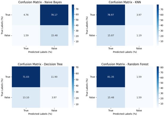
Figure 2.
Graphical presentation of the confusion matrix values for the mental health dataset.
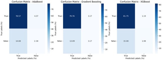
Figure 3.
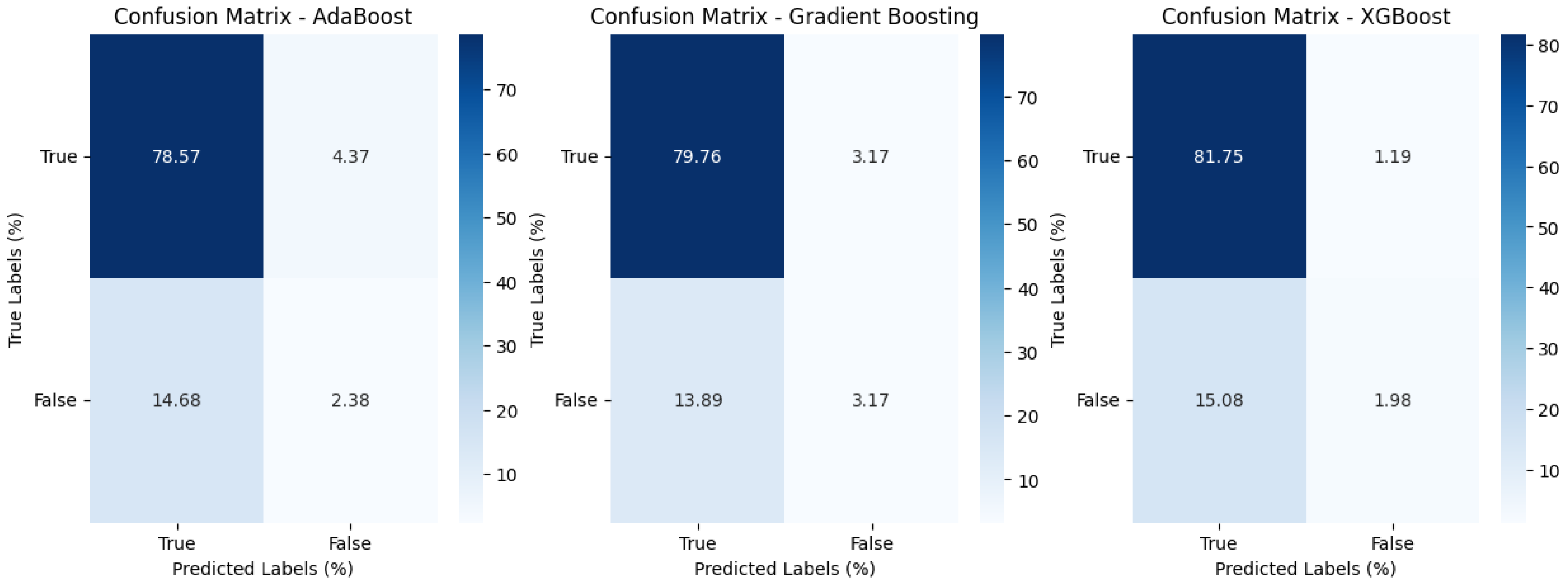
Graphical presentation of the confusion matrix values for the mental health dataset (boosting algorithms).
The observed confusion matrix shows a noteworthy rate of false negatives (1.59%) and a relatively higher rate of true positives (4.76%). These findings suggest that naive Bayes exhibits high sensitivity when identifying positive cases, implying a lower specificity for distinguishing negative cases.
Turning our attention to the K-nearest neighbors (KNN) model, a high number of true positives (78.97%) and a lower rate of false positives (3.97%) were observed. This indicates that KNN is proficient at identifying positive cases, but can occasionally misclassify negative cases as positive.
When analyzing the confusion matrix results for the decision tree model, the percentages of true negatives (3.97%), false positives (11.90%), false negatives (13.10%), and true positives (71.03%) were observed. These findings suggest that the decision tree model demonstrates a relatively high true-positive rate and notable false-positive and false-negative rates in its predictions.
In the case of random forest, the second highest rate of true positives (81.35%) and a low rate of false positives (1.59%) were observed. However, the model also exhibited a relatively high rate of false negatives (15.48%), indicating that, while it exceled at correctly identifying positive cases, it struggled with missing some actual positive instances, potentially affecting its overall performance in specific applications.
Shifting the focus to AdaBoost, a relatively high rate of false negatives (14.68%) and a relatively high rate of true positives (78.57%) were found. This suggests that the AdaBoost model is effective in correctly identifying positive cases, but may need improvement in reducing the number of false negatives to enhance its overall performance.
Similarly, the gradient boost model displayed a relatively high rate of false negatives (13.89%) and a high rate of true positives (79.76%). These results indicate that the model excels at correctly identifying positive cases, but can benefit from further optimizations to reduce the occurrence of false negatives and enhance its overall performance.
Finally, when examining XGBoost, the smallest rate of false positives (1.19%) and the highest rate of true positives (81.75%) were observed. This suggests that XGBoost is particularly effective at minimizing false-positive errors and excels at correctly identifying positive cases, making it a strong candidate for tasks where precision is crucial.
Comparing the confusion matrix metrics across these classification models, it can be observed that each model has its strengths and weaknesses. While some models can excel in correctly identifying positive cases, they can miss out on some negative cases. On the other hand, some models can accurately identify negative cases, but also tend to misclassify negative cases as positive. These variations highlight the importance of carefully considering the specific characteristics of the dataset and the desired classification goals when selecting an appropriate model.
The analysis of feature importance in the dataset, as seen in Figure 4, conducted using a random forest classifier, provided valuable insights into the factors that wielded the most substantial influence when it came to predicting mental health consequences. These findings are essential for understanding the dynamics of mental health in the workplace and can inform strategies for better support and intervention.
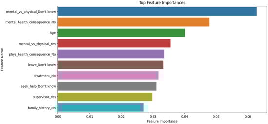
Figure 4.
Graphical presentation of feature importance using the random forest algorithm for the mental health dataset.
The mental_vs_physical feature is at the top of the list of influential features, with an importance value of approximately 6.28%. This suggests that employees who are uncertain or unaware of their company’s stance regarding mental health benefits are more likely to experience mental health problems. This uncertainty appears to be a significant contributing factor.
The mental_health_consequence feature follows closely behind, with an importance value of about 4.78%. This feature indicates that individuals who perceive no mental health consequences in their workplace environment are less likely to face such issues. It underscores the roles of awareness and perception in shaping mental health outcomes.
Age, a fundamental demographic factor, is another significant predictor, with an importance value of around 4.01%. This suggests that age plays a role in determining mental health outcomes, with different age groups experiencing varying levels of mental health challenges. It highlights the need for age-sensitive mental health support strategies.
6.2. The Evaluation of the Second Dataset: Loan Approval
The outcomes obtained from the implementation of the algorithms on the second dataset reveal notable disparities in the accuracy among the various models. The random forest, AdaBoost, gradient boost, and XGBoost algorithms demonstrate significantly superior accuracy results in comparison to the naive Bayes and KNN models. Random forest achieved the highest accuracy scores, reaching an impressive value of 85%.
Random forest also exhibited the highest precision score of 86%, closely followed by the decision tree and KNN algorithms with a score of 80%. These results accentuate the models’ adeptness of accurately classifying positive instances, thereby implying their efficacy in minimizing false positives.
Regarding recall, which measures a model’s capability to capture all pertinent positive instances, the highest recall score is 83%. Considering these findings presented in Table 6, it can be deduced that the random forest algorithm represents the premier-performing algorithm across all four evaluation metrics—accuracy, precision, recall, and F1 score.
Table 6.
Model’s metrics results for the second dataset.
The confusion matrix results, as shown in Figure 5 and Figure 6 and Table 7, present XGBoost as the top-performing algorithm, boasting a high true-positive rate of 53.96%. However, it is important to note that XGBoost also exhibits the highest false-negative rate of 39.01%, which means it excels at correctly identifying positive cases but can miss out some true positives, potentially requiring further optimizations in certain scenarios.
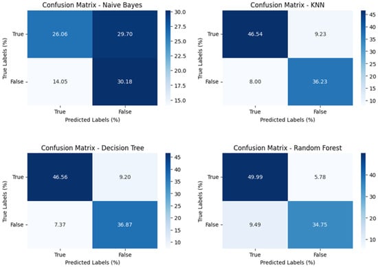
Figure 5.
Graphical presentation of the confusion matrix values for the loan approval dataset.
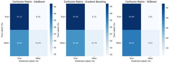
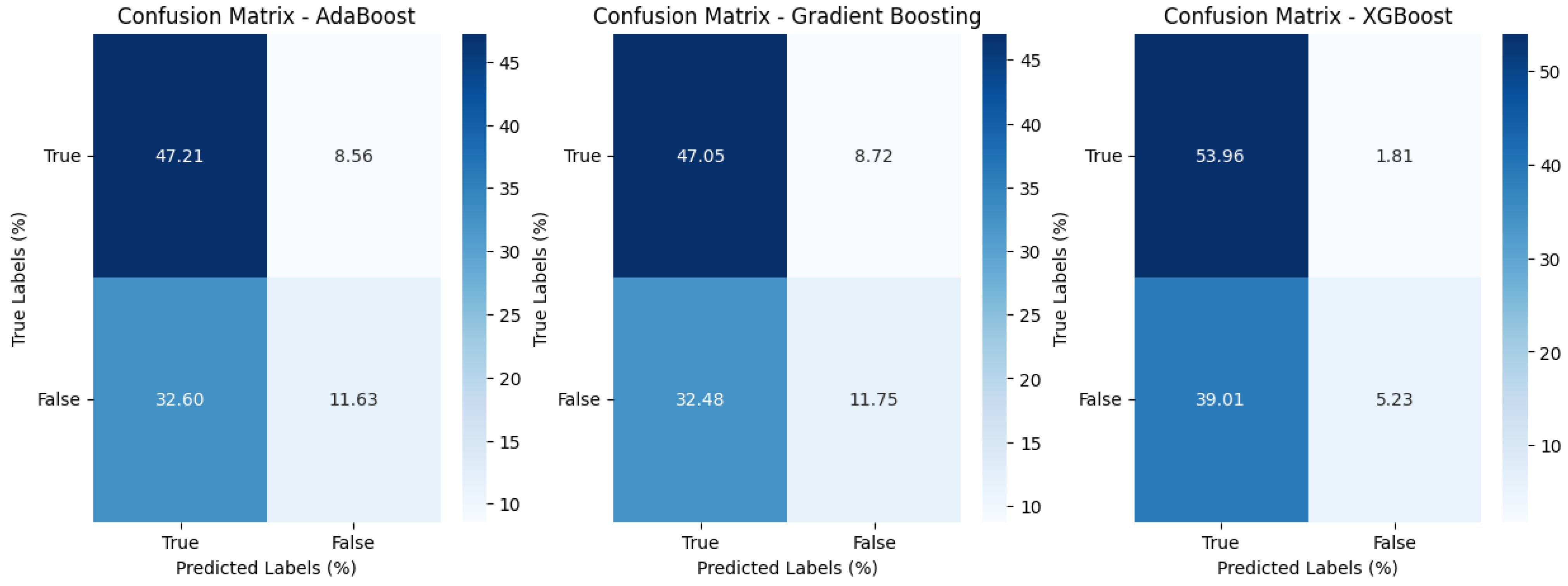
Figure 6.
Graphical presentation of the confusion matrix values for the loan approval dataset (boosting algorithms).
Table 7.
Confusion matrix results for the second dataset.
The gradient boost model achieved a true-positive rate of 47.05% and a true-negative rate of 11.75%. Similarly, the AdaBoost model exhibited a true-positive rate of 47.21% and a true-negative rate of 11.16%. This indicates that both models are fairly adept at correctly identifying positive cases while also maintaining a reasonable ability to correctly identify negative cases.
In contrast, the naive Bayes model displayed the poorest performance in terms of true-positive and true-negative rates, achieving a meager true-positive rate of only 26.06% and a true-negative rate of 30.18%. On the other hand, the decision tree and random forest models showcased relatively robust performances, with true-positive rates of 46.56% and 49.99%, respectively.
On the whole, considering the evaluation of true-positive and true-negative rates, as well as false-positive and false-negative rates, the decision tree and random forest algorithms emerged as the optimal algorithms in this comparative analysis. These models demonstrated high rates of correctly identifying positive and negative instances, while also exhibiting relatively low rates of misclassifications. These findings suggest that decision tree and random forest models have the most favorable balance between accurately detecting positive and negative instances while minimizing erroneous classifications.
The analysis of feature importance in the dataset, as shown in Figure 7, utilizing a model, highlighted key factors that significantly influenced the outcomes. Age emerged as the most dominant feature, with an importance score of approximately 16.28%, indicating its substantial impact on the predicted results.
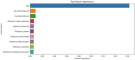
Figure 7.
Graphical presentation of feature importance using the random forest algorithm for the loan approval dataset.
Other features, such as Car_Ownership (both yes and no categories), and various professions, like flight attendant, physician, drafter, psychologist, web designer, and secretary, also played a role in influencing the outcomes to a lesser extent.
In summary, age stood out as the primary driver, while certain professions and car ownership status also exhibited an influence on the results. These findings provide valuable insights for understanding the factors affecting the predicted outcomes of the dataset.
7. Discussion
Sujatha et al. (2021) [30], Tumuluru et al. (2022) [31], and Mamun et al. (2022) [32] used different machine learning algorithms and techniques to predict loan approvals. However, despite the differences in the methodologies, all three studies used supervised learning algorithms to predict loan approvals.
Sujatha et al. (2021) [30] used four machine learning algorithms, namely, logistic regression, decision tree, random forest, and KNN, to predict loan approvals. With the use of data preprocessing techniques in their study, such as missing value imputation, feature scaling, and encoding categorical variables, the logistic regression algorithm achieved the highest accuracy of 84.55%, followed by the random forest, decision tree, and KNN algorithms, with accuracy scores of 80.49%, 70.73%, and 65.04%, respectively. The authors attribute the high accuracy to the fact that logistic regression is a linear model, which is more suitable for this kind of problem where there is a clear boundary between the classes.
Tumuluru et al. (2022) [31] also used data preprocessing techniques, such as feature scaling, normalization, and one-hot encoding, as well as four machine learning algorithms, namely, logistic regression, random forest, k-nearest neighbor, and support vector machine, to predict loan approvals. They found that random forest had the highest accuracy of 81%, followed by logistic regression (77%), SVM (73.2%), and KNN (68%). The authors attributed the success of the random forest algorithm to the fact that it was an ensemble learning algorithm that combined multiple decision trees, which could achieve a better performance than individual decision trees.
Mamun et al. (2022) [32] used six machine learning algorithms, namely, XGBoost, AdaBoost, LightGBM, decision tree, random forest, and KNN, to predict loan approvals. They used data preprocessing techniques, such as feature scaling, missing value imputation, and encoding categorical variables. The authors found that LightGBM had the highest accuracy of 91.89%, followed by random forest with an accuracy of 91.88%, then XgBoost, AdaBoost, and KNN with accuracies of 91%, 91.87%, and 91.67%, respectively. The lowest accuracy of 84.97% belonged to the decision tree algorithm. The authors attributed the high accuracy of the random forest algorithm to its ability to handle both linear and non-linear relationships between the features and the target variable.
These findings are consistent with the results obtained in this study. However, it is important to note that, in this paper, the models were evaluated using additional metrics, such as recall, precision, and F1 score, which provided a more comprehensive evaluation of the models’ performances.
One limitation of the abovementioned studies was that they did not consider the interpretability of the models. While machine learning models show high accuracy outcomes when predicting loan approvals, their lack of interpretability makes it difficult to understand how they make decisions. As a result, it can be challenging to explain to customers why their loan applications are accepted or rejected.
Another limitation was that these studies did not consider the impact of the imbalanced dataset. In the loan approval prediction, the number of rejected loan applications was often higher than the number of approved applications. This imbalance can affect the accuracy of the models and can lead to biased predictions. Future research should explore the methods for addressing imbalanced datasets and improving the interpretability of the models.
Although the accuracy of the models varied depending on the used algorithms, all three studies achieved high accuracy results when predicting loan approvals. The findings of these studies can help banks and financial institutions make informed decisions and reduce the risk of defaults. However, the interpretability and the impact of imbalanced datasets need to be considered in future research.
When handling mental health data in the context of credit risk prediction in the European Union, it is imperative to adhere to the General Data Protection Regulation (GDPR), a comprehensive legal framework effective from 25 May 2018. Several key articles within the GDPR are particularly relevant to the processing of sensitive personal data, including mental health information.
Article 6 of the GDPR addresses the lawfulness of processing personal data. Consent (Article 6(1)(a)), the necessity of processing for the performance of a contract (Article 6(1)(b)), and compliance with a legal obligation (Article 6(1)(c)) are examples of legal bases applicable to the processing of mental health data.
Article 9 specifically deals with the processing of special categories of personal data, including health data. Article 9(2)(a) permits processing with explicit consent, while 9(2)(b) allowing the processing to carry out tasks in the field of employment and social security.
Article 5 outlines the principles of data processing, including data minimization (Article 5(1)(c)) and the integrity and confidentiality of processing (Article 5(1)(f)), both crucial considerations when handling mental health data.
Recital 22 provides an additional context regarding the conditions for processing special categories of personal data. It emphasizes the need for explicit consent and underscores the importance of safeguarding individual rights.
While the GDPR does not explicitly mention credit risk prediction, its conditions regarding the processing of special categories of personal data, such as mental health information, are applicable across various contexts. Therefore, organizations, including banks, must adhere to the principles and requirements outlined in these relevant articles of the GDPR when implementing systems involving mental health data for credit risk prediction.
8. Conclusions
This study aimed to demonstrate the potential to revolutionize the evaluation of borrowers’ creditworthiness by financial institutions by integrating mental health data as an important predictor variable in the loan approval process. The supervised machine learning algorithms used in this research showcased superior performances in accurately identifying individuals with a higher risk of defaulting on their loans. For instance, the XGBoost algorithm achieved the highest accuracy of 84% in the first dataset, surpassing gradient boost (83%) and KNN (83%). In the second dataset, the random forest algorithm achieved the highest accuracy of 85%, followed by the decision tree and KNN algorithms with 83%.
In comparison to the studies discussed in the previous section, this study utilized a similar data preprocessing approach, with techniques, such as feature scaling and one-hot encoding. However, the missing value imputation was not performed as the dataset used in this paper did not have any missing values. Additionally, different sets of machine learning algorithms, including naive Bayes and AdaBoost, were used in this study, which achieved lower accuracy scores compared to the other models. This could be attributed to the underlying algorithms’ limitations, as previously discussed.
The findings of this paper align with the previous studies showing that machine learning algorithms can achieve high accuracy results when predicting loan approvals. However, it is important to consider the limitations of the models, such as their lack of interpretability and the impact of imbalanced datasets. Future studies should focus on developing more accurate predictive models by incorporating additional variables related to the mental health states of borrowers, such as stress levels, anxiety, and depression.
Another important area of research pertains to the ethical considerations surrounding the use of mental health data in the loan approval process. While the integration of these data can improve decision making, this raises valid concerns regarding privacy and discrimination.
Adhering to the General Data Protection Regulation (GDPR) is crucial when handling mental health data for credit risk predictions in the European Union. Key GDPR articles, including those addressing the lawfulness of processing personal data (Article 6) and special categories, like health data (Article 9), emphasize obtaining explicit consent and safeguarding individual rights. Organizations, including banks, must follow these GDPR provisions when utilizing mental health data for credit risk predictions, despite the absence of explicit mentions of credit risk predictions in the GDPR.
Therefore, future investigations should also address the development of ethical guidelines and policies to ensure the responsible use of mental health data in the loan approval process.
Future research should explore the methods for improving the interpretability of the models and addressing imbalanced datasets to improve the models’ performances.
In conclusion, the numerical results obtained in this study highlight the superior performance of supervised machine learning algorithms, such as random forest, when accurately predicting loan default risks based on mental health data. These findings indicate the potential benefits for financial institutions of adopting machine learning algorithms in their loan approval processes, particularly when evaluating borrowers with mental health issues. By embracing these advancements, financial institutions can enhance their risk assessment capabilities and make more informed lending decisions.
Author Contributions
Conceptualization, E.K., D.H., A.A., M.D. and N.H.; methodology, E.K., A.A., M.D. and N.H.; software, A.A., D.H. and M.D.; validation, D.H., E.K., A.A. and M.D.; formal analysis, D.H., E.K., N.Z., A.A., M.D., N.H. and E.S.; investigation E.K., A.A. and M.D.; resources, E.K., A.A., M.D. and N.H.; data curation, D.H., A.A., M.D. and N.H.; writing—original draft preparation, A.A., N.H. and M.D.; writing—review and editing, D.H., E.K., N.Z., A.A., M.D. and N.H.; visualization, D.H., E.K. and N.H.; supervision, D.H., E.K., N.Z. and E.S.; project administration, E.K. and N.H.; funding acquisition, N.Z. and E.S. All authors have read and agreed to the published version of the manuscript.
Funding
This research received no external funding.
Institutional Review Board Statement
Not applicable.
Informed Consent Statement
Not applicable.
Data Availability Statement
Data are contained within the article.
Conflicts of Interest
The authors declare no conflict of interest.
References
- Prabaljeet, S.S.; Atush, B.; Lekha, R. Loan Approval Prediction Using Machine Learning: A Comparative Analysis of Classification Algorithms. 2023. Available online: https://ieeexplore.ieee.org/document/10182799/authors#authors (accessed on 19 December 2023).
- Yash, D.; Prashant, R.; Pratik, C. Loan Approval Prediction Using Machine Learning. 2021. Available online: https://www.irjet.net/archives/V8/i5/IRJET-V8I5331.pdf (accessed on 19 December 2023).
- Mohammad, A.S.; Amit, K.G.; Tapas, K. An Approach for Prediction of Loan Approval Using Machine Learning Algorithm. 2020. Available online: https://ieeexplore.ieee.org/document/9155614 (accessed on 19 December 2023).
- Almheiri, A.S. Automated Loan Approval System for Banks. Rochester Institute of Technology, Dubai. 2023. Available online: https://scholarworks.rit.edu/cgi/viewcontent.cgi?article=12535&context=theses (accessed on 19 December 2023).
- Banco de España, Eurosistema. Report on the Financial and Banking Crisis in Spain, 2008–2014. 2017. Available online: https://repositorio.bde.es/bitstream/123456789/15112/1/InformeCrisis_Completo_web_en.pdf (accessed on 19 December 2023).
- How Much Does Racial Bias Affect Mortgage Lending? Evidence from Human and Algorithmic Credit Decisions—Neil Bhutta, Aurel Hizmo, Daniel Ringo. Available online: https://www.federalreserve.gov/econres/feds/files/2022067pap.pdf (accessed on 19 December 2023).
- Roberts, R. Mental Health and Money: A Practical Guide; Money and Mental Health Policy Institute: London, UK, 2019. [Google Scholar]
- Bhargav, P.; Sashirekha, K. A Machine Learning Method for Predicting Loan Approval by Comparing the Random Forest and Decision Tree Algorithms. 2023. Available online: https://sifisheriessciences.com/journal/index.php/journal/article/view/414/397 (accessed on 19 December 2023).
- Wang, Y.; Wang, M.; Yong, P.; Chen, J. Joint loan risk prediction based on deep learning-optimized stacking model. Eng. Rep. 2023, e12748. [Google Scholar] [CrossRef]
- Abdullah, M.; Chowdhury, M.A.F.; Uddin, A.; Moudud-Ul-Huq, S. Forecasting nonperforming loans using machine learning. J. Forecast. 2023, 42, 1664–1689. [Google Scholar] [CrossRef]
- Alsaleem, M.Y.E.; Hasoon, S.O. Predicting bank loan risks using machine learning algorithms. AL-Rafidain J. Comput. Sci. Math. 2020, 14, 159–168. [Google Scholar] [CrossRef]
- World Health Organization. Mental Disorders. 2019. Available online: https://www.who.int/health-topics/mental-disorders#tab=tab_1 (accessed on 19 December 2023).
- National Alliance on Mental Illness. Mental Health by the Numbers. 2021. Available online: https://www.nami.org/mhstats (accessed on 19 December 2023).
- Mental Health America. The State of Mental Health in America. 2021. Available online: https://mhanational.org/sites/default/files/2021%20State%20of%20Mental%20Health%20in%20America_0.pdf (accessed on 19 December 2023).
- Mental Health First Aid USA. About Mental Health First Aid. 2021. Available online: https://www.mentalhealthfirstaid.org/about/ (accessed on 19 December 2023).
- Javed, K.; Hamid, F. A comparative study of decision tree algorithms for nonlinear and complex relationships between input features and output variables. Int. J. Adv. Res. Comput. Sci. Softw. Eng. 2015, 29, 65–74. [Google Scholar]
- Breiman, L.; Friedman, J.; Stone, C.J.; Olshen, R.A. Classification and Regression Trees; Taylor & Francis: Abingdon, UK, 1984. [Google Scholar]
- Niculescu-Mizil, A.; Caruana, R. Predicting good probabilities with supervised learning. In Proceedings of the 22nd International Conference on Machine Learning, Bonn, Germany, 7–11 August 2005. [Google Scholar]
- Shahriari, B.; Swersky, K.; Wang, Z.; Adams, R.P.; de Freitas, N. Taking the human out of the loop: A review of Bayesian optimization. In Proceedings of the IEEE; IEEE: Piscataway, NJ, USA, 2016. [Google Scholar]
- Kaviani, P.; Dhotre, M.S. Short Survey on Naive Bayes Algorithm. Int. J. Adv. Res. Comput. Sci. Manag. 2017, 4, 44839. [Google Scholar] [CrossRef]
- Jena, B. Gender Recognition of Speech Signal using KNN and SVM. SSRN Electron. J. 2021. [Google Scholar] [CrossRef]
- Zhan, Y.; Liu, J.; Gou, J.; Wang, M. A video semantic detection method based on locality-sensitive discriminant sparse representation and weighted KNN. J. Vis. Commun. Image Represent. 2016, 41, 65–73. [Google Scholar] [CrossRef]
- Syaliman, K.U.; Labellapansa, A. Improving the Accuracy of Features Weighted k-Nearest Neighbor Using Distance Weigh; SciTePress: Setúbal, Portugal, 2019. [Google Scholar]
- Freund, Y.; Schapire, R.E. Boosting: Foundations and Algorithms; The MIT Press: Cambridge, MA, USA, 2013. [Google Scholar]
- Shahri, N.H.N.B.M.; Lai, S.B.S.; Mohamad, M.B.; Rahman, H.A.B.A.; Bin Rambli, A. Comparing the Performance of AdaBoost, XGBoost, and Logistic Regression for Imbalanced Data. Math. Stat. 2021, 9, 379–385. [Google Scholar] [CrossRef]
- Friedman, J.H. Greedy function approximation: A gradient boosting machine. Ann. Stat. 2001, 29, 1189–1232. [Google Scholar] [CrossRef]
- Masui, T. All You Need to Know about Gradient Boosting Algorithm—Part 1. Regression. 2022. Available online: https://towardsdatascience.com/all-you-need-to-know-about-gradient-boosting-algorithm-part-1-regression-2520a34a502 (accessed on 19 December 2023).
- Chen, T.; Guestrin, C. XGBoost: A scalable tree boosting system. In Proceedings of the 22nd ACM SIGKDD International Conference on Knowledge Discovery and Data Mining, San Francisco, CA, USA, 13–17 August 2016. [Google Scholar]
- Ke, G.; Meng, Q.; Finley, T.; Wang, T.; Chen, W.; Ma, W.; Ye, Q.; Liu, T.-Y. LightGBM: A highly efficient gradient boosting decision tree. In Proceedings of the 31st International Conference on Neural Information Processing Systems, Long Beach, CA, USA, 4–9 December 2017. [Google Scholar]
- Sujatha, C.N.; Gudipalli, A.; Pushyami, B.H.; Karthik, N.; Sanjana, B.N. Loan Prediction Using Machine Learning and Its Deployment on Web Application. In Proceedings of the 2021 Innovations in Power and Advanced Computing Technologies (i-PACT), Kuala Lumpur, Malaysia, 27–29 November 2021. [Google Scholar]
- Tumuluru, P.; Burra, L.R.; Loukya, M.; Bhavana, S.; CSaiBaba, H.M.H.; Sunanda, N. Comparative Analysis of Customer Loan Approval Prediction using Machine Learning Algorithms. In Proceedings of the Second International Conference on Artificial Intelligence and Smart Energy (ICAIS-2022), Coimbatore, India, 23–25 February 2022. [Google Scholar]
- Mamun, M.A.; Farjana, A.; Mamun, M. Predicting Bank Loan Eligibility Using Machine Learning Models and Comparison Analysis. In Proceedings of the 7th North American International Conference on Industrial Engineering and Operations Management, Orlando, FL, USA, 12–14 June 2022. [Google Scholar]


Disclaimer/Publisher’s Note: The statements, opinions and data contained in all publications are solely those of the individual author(s) and contributor(s) and not of MDPI and/or the editor(s). MDPI and/or the editor(s) disclaim responsibility for any injury to people or property resulting from any ideas, methods, instructions or products referred to in the content. |
© 2024 by the authors. Licensee MDPI, Basel, Switzerland. This article is an open access article distributed under the terms and conditions of the Creative Commons Attribution (CC BY) license (https://creativecommons.org/licenses/by/4.0/).