Effective Data Reduction Using Discriminative Feature Selection Based on Principal Component Analysis

Abstract

Effective data reduction must retain the greatest possible amount of informative content of the data under examination. Feature selection is the default for dimensionality reduction, as the relevant features of a dataset are usually retained through this method. In this study, we used unsupervised learning to discover the top-k discriminative features present in the large multivariate IoT dataset used. We used the statistics of principal component analysis to filter the relevant features based on the ranks of the features along the principal directions while also considering the coefficients of the components. The selected number of principal components was used to decide the number of features to be selected in the SVD process. A number of experiments were conducted using different benchmark datasets, and the effectiveness of the proposed method was evaluated based on the reconstruction error. The potency of the results was verified by subjecting the algorithm to a large IoT dataset, and we compared the performance based on accuracy and reconstruction error to the results of the benchmark datasets. The performance evaluation showed consistency with the results obtained with the benchmark datasets, which were of high accuracy and low reconstruction error.

1. Introduction

Data have become ubiquitous with the advances in technology, leading to the collection of heterogeneous big data in every field imaginable. This makes it difficult for pattern discoveries to be made due to the presence of noise and redundant data. For effective data exploration, one must find a way to reduce noise and redundant data and be able to select relevant features for pattern discovery and analysis [1]. This experiment has applications in the pursuit of smart cities and edge computing that rely on the IoT and edge devices that generate big data but have low computing resources for data processing. Therefore, one must find ways to reduce the data volume to a size that is suitable for these devices without compromising efficiency and accuracy.

Most dimensionality reduction algorithms and experiments rely on feature selection and feature extraction to discover underlying patterns in data [2,3]. This preserves the underlying framework of the original data while generating a new or reduced dataset. Although both feature extraction and feature selection reduce the size of the data, their methodologies differ. While feature selection attempts to identify relevant features in a dataset using methods such as entropy, information gain, univariate/multivariate feature selection, etc., feature extraction attempts to build a new set of features from the original dataset in a new feature space that will yield low dimensions, and this helps the applicable algorithms to fit better [4]. Both methods are necessary to reduce the challenges associated with memory and computing costs, which are a real concern in the IoT environment.

In conducting this research, our intent is to enhance the ability of edge devices to store and analyze big data by reducing the data volume they handle while not compromising quality. The need for edge computing resources to meet the needs of low-latency edge services is driving firms toward the extensive deployment of edge and fog computing resources. With self-driving vehicle adoption and smart city inevitability, scientists must find ways to process edge-generated data at the edge, and this means finding ways to reduce the volume of edge-generated data without compromising efficiency and the underlying information needed for analysis and decision-making.

Our proposed method uses both feature selection and feature extraction. We leveraged the statistical work of principal component analysis (PCA) to identify the feature ranks along the principal direction, considering the values of the coefficient of the principal direction [5]. We used singular value decomposition (SVD) for feature extraction, having selected a good percentage of the features that efficiently represent the original data. The beauty of this work is that no feature is dropped per se, as all of the components are considered in PCA, which is a data reduction algorithm. Feature selection considers the feature weight score of the class and makes decisions to drop a feature based on a chosen threshold.

The work carried out in this study adapted the research work of Aminata Kane et al. [6]. By building on their work, we investigated what number of principal components (PCs) would suit the data reduction needs of IoT devices, and we subjected the model to a large real industry dataset to test its effectiveness. Most businesses adapting PCA for reduction and analysis purposes usually choose the top five PCs. However, this may not work best for many datasets, depending on the insights, level of accuracy desired, and characteristics of the data.

Some of the pros of dimensionality reduction include the benefit of less computation and training time [7]. The same benefit also accrues as redundancy is removed. Other benefits include less storage space being required. The dataset becomes flexible for 2D and 3D plotting and also improves for ease of interpretation. Dimensionality reduction also helps to filter out the most significant features, leaving the less significant.

2. Literature Review

Significant research has been carried out in the field of feature selection and dimensionality reduction [8,9,10,11] in the search for different algorithms that can preprocess data for a reduced, content-rich dataset that will be useful for different analytical purposes. This, however, has not solved all of the challenges that exist in the field of data reduction.

A closely adapted research work by Aminata Kane et al. [6] involved the application of PCA and SVD similarly on many benchmark datasets, and the authors compared their results to the results of other experiments on the same datasets, making a case for their method. In their work, they compared their PCA-selected number of components to other feature selection experiments and compared their SVD results to the results of the other experiments examined.

Understanding the factors on which feature selection is built is important in developing a good feature selection algorithm. Herve Nkiama et al., in their work [12], employed a recursive feature selection algorithm that is based on a tree classifier to uncover relevant features. The tree classifier tries to remove non-relevant features by weighing the score of each feature to the class label. The results improved the intrusion detection capabilities of the system based on the NSL-KDD dataset.

In [13], Lukman Hakim et al. also examined the influence of feature selection on network intrusion detection using the NSL-KDD dataset. It was duly noted that the presence of irrelevant features in a dataset decreases the accuracy and performance of the system. In their work, the feature selection algorithms used were based on information gain, gain ratio, chi-squared, and relief selection using known algorithms that include J48, Random Forest, KNN, and Naïve Bayes. While they observed an improvement in the detection system, there was a slight decrease in accuracy.

Feature selection methods can be grouped into two classes: supervised and unsupervised. Fisher score [5] or ReliefF [14] methods evaluate feature importance by exploring the dependence that exists between features and the label class. These methods assume class labels as data. The difficulty with this is that it becomes very difficult to enforce this assumption with high-dimensional data, which makes it is very difficult to obtain the labels. Methods such as leverage score sampling [6], which falls into the unsupervised method of feature selection, use all of the features to uncover the hidden relationships or patterns that exist within the dataset and leverage them to classify the data.

In [15], the considered techniques depended on locality-preserving features. This type of method seeks to classify data by grouping them into k-nearest neighbors to retain features that represent the tree structure.

Another set of methods was examined to select features that most represent the dataset. The most representative features would contain most of the information present in the dataset. One such method is the PCA algorithm, which Joliffe, in [16], utilized in analyzing different algorithms. This method is based on statistical calculations that show that the selection of features is associated with their principal components and the absolute value of their coefficients. This is partly the method adopted in this work.

Some machine learning algorithms have also been effectively used in feature selection, with them using different metrics for decision-making. The authors of [17] used the JRip machine learning algorithm, which is performance-based, to implement feature selection in their dimensionality reduction experiment to improve the effectiveness of their system.

Abhishek et al. [18], in their evaluation of the KDD dataset, explored different methods in the evaluation of the effectiveness of the KDD dataset for anomaly-based intrusion detection. They used different machine learning algorithms in their evaluation and compared their results to the performance of the UNSW-NB15 dataset, proposing the latter as a better alternative for NID experiments. The focus of their work highlights the importance of proper feature distribution in a dataset for good model performance. The authors of [13], performing their own experiments on the KDD dataset, observed that feature selection significantly improved the performance of the NIDS system, though with a slight reduction in accuracy.

3. Study Background

This section explains the dataset used, the research concepts, and the problem statement.

3.1. Brief Overview of the Datasets

The relevant background information about the datasets used in this work is explained in this section. This includes a brief overview of the datasets, principal component analysis (PCA), and singular value decomposition (SVD).

Datasets

Five benchmark datasets were used in this experiment to evaluate the performance of the proposed methodologies. Additional real-time big data from the IoT were included in the experiment to evaluate the response of the method to real data from the industrial space.

The benchmark datasets include:

i.

The Arrhythmia Dataset: This dataset was generated to predict the presence or absence of cardiac arrhythmia and classify the cardiac arrhythmia within the 16 classes of the dataset [19].

ii.

The Madelon Dataset: The Madelon Dataset was generated as AI data that contains data points that are grouped into 32 clusters that are placed on the vertices of hypercubes with five dimensions and are labeled randomly as +1 or −1. These five dimensions represent features with information, while 15 additional linear combinations of the informative features were added to make this number 20, with the 15 being redundant. The goal of the experiment is to classify the 20 features into +1 and −1. Probe features were added to the dataset as distractions, with them holding no prediction power. They served as distractions to test the power of the algorithm [20].

iii.

The Gissette Dataset: This is one of the five datasets that was used in the NIPS 2003 challenge for feature selection. The dataset is made up of a fixed-sized dimensional image of 28 × 28 containing digits that are size-normalized and that are placed at the center of the image. The images contain pixel features that were sampled randomly at the middle–top of the features that contain the necessary information to identify four from nine, and higher dimensional features were created from these features to cast the challenge to a higher dimensional feature space. Features that serve as a distraction were added, with them being called probes and having no power in prediction [21].

iv.

The Ionosphere Dataset: This is a radar dataset with targets as free electrons present in the ionosphere. The class is such that ‘good’ radar should return some evidence that contains a specific kind of structure in the ionosphere, while ‘bad’ radar does not return such structural evidence [22].

v.

The IoT Intrusion Data: This is a large proprietary IoT dataset, with intrusions having 115 features. A fraction was used due to volume and computing speed constraints, giving a subset of 80,037 samples and 115 features.

The features of the datasets are expressed in the

Table 1. Dataset features and samples.

Dataset	N_Samples	N_Features	Class
Arrhythmia	452	279	16
Ionosphere	351	34	2
Madelon	2000	502	2
Gissette	5999	5000	2
IoT Intrusion	80,037	115	5

.

3.2. Principal Component Analysis (PCA)

The emergence of big data collection in every sector of industry presents difficulties in interpretation. This is where PCA [2,4,8] comes to the rescue by reducing the dimensionality of datasets without sacrificing information. This enhances the interpretability of the dataset, including all of the benefits of dimensionality reduction. Principal component analysis builds new features by projecting the features to new planes that are orthogonal to each other. The distributions of the features in planes enhance the interpretability of the relationship between the features.

Some key terminologies regarding PCA that aid its comprehension include the following:

• View—The perspective (angle of sight) through which the data points are viewed (observed).
• Dimension—The columns in a dataset. This is the same as the feature.
• Projections—This is the perpendicular distance that exists between the data points and the principal components.
• Principal Components—These are the new variables that are constructed as linear combinations or mixtures of the supplied initial variables.

Therefore, it becomes clear that the number of principal components will always be less than or equal to the number of initial variables. The principal components are always orthogonal, and the priority of the PCs decreases as their number increases from PC₁ to PC_N. When given a dataset, principal component analysis performs the following operations on the dataset in the following correct order—standardization, covariance matrix computation, eigenvector, and eigenvalue computation—and generates feature vectors [6,16].

Standardization manipulates the data points to fall within similar boundaries [23].

Z = (x − ẋ)/std.

In the covariance matrix computation [24], the correlation between any two or more attributes in a multidimensional dataset is expressed. The matrix entries are the covariance and variance of the feature values. Figure 1 and Figure 2 shows the covariance matrix of two features and n features respectively.

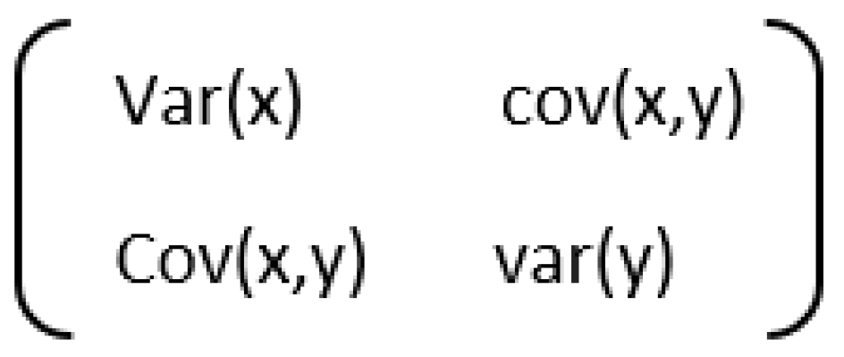
3.3. Singular Value Decomposition (SVD)

The singular value decomposition of any given matrix A is the decomposition of that matrix into a product of three different matrices expressed as A = UDV^T, where D is a diagonal matrix with positive real values and U and V have columns that are orthonormal.

One of the applications of SVD is in the approximation of data where a data matrix A is expressed as a matrix of low ranks, and we found the low-rank matrix that is a good approximation of the data matrix. That is, with a data matrix A, we can find a low-rank matrix B, which is a perfect approximation of the data matrix A. In the expression above, U and V are the left and right singular vectors, while D is a diagonal matrix. Matrix A can be expressed as below [25] in Figure 3.

$$\mathrm{A}=U{\sum }_i{V}^T$$

In this expression, i ≤ min{m, n} denotes the rank of A, U_i ∈ R^m×ρ is an orthonormal matrix, D_i is an i × i diagonal matrix, and V_i ∈ R^n×i is an orthonormal matrix.

3.4. Problem Statement

A multivariate time series data A_n,m of n instances with m variables, Figure 4, may be presented as an n × m matrix A having t_i; _j is the value of the variable v_j measured at time i, with it having 1 ≤ i ≤ n, 1 ≤ j ≤ m [6].

The goal at this point is to find and select the most informative features within the data matrix of n instances and m features while preserving the intrinsic structure of the dataset using unsupervised feature selection methods [27]. The selected features should be able to represent the original dataset with the subset features [28].

Let A be a matrix of n × m, with n instances and m features. We search for a subset S of n × k, where k < m (column selection), which will retain the characteristics of the original dataset [6]. A column subset selection will uncover the most k informative columns of A in such a way that the |A − CC^TA| will be minimized over all possible combinations k for C that can be obtained from m of A. CC^T will represent the projection of K-dimensional space that is amassed by the columns of C, ξ = {2, F} will denote the spectral norm and Frobenius norm, respectively, and the Moore–Penrose pseudo-inverse of C will be C^T [16,29].

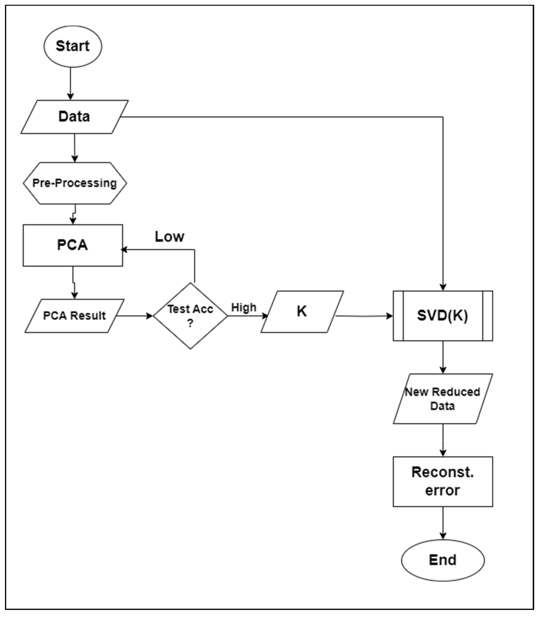
4. Proposed Methodology

The goal in this case is to find a subset matrix C_n,k from A_n,m such that k < m. Let V_k be the singular vector containing the top-k features of A, with r = rank(A), r <= {n, m}, and k < r. The algorithm for the top-k feature selection and the generation of a new dataset is given below.

The system diagram for the proposed methodology is shown below in Figure 5.

Algorithm

• Data exploration—explore the data to check their features and balance.
• Data preprocessing—perform data cleaning and train/test set division.
• PCA implementation—perform PCA transformation, selecting N-components such that the dataset A_n,m >> X_k,m.
• Test the accuracy with a model and repeat until the best N-components (top-K features) are realized.
• Implement SVD using the chosen N-component numbers.
• A new dataset is produced.
• Test the new dataset with a model to test the accuracy.
• Calculate the reconstruction error.

The steps above define all of the steps in the proposed method. The method relies on statistical deductions of principal component analysis [29] to select principal components with high priority that represent the dataset to a good degree. This representation is verified using different machine learning algorithms to test the accuracy of the representation against the class. The top-k selected principal components become the guide to selecting the feature vectors from the SVD algorithm, hence the use of feature reduction and selection methods.

The method is used on benchmark datasets and then a real-life big dataset to test the performance of the proposed method.

5. Performance Evaluation, Results, and Discussion

This section discusses the metrics used to evaluate the performance of the experiment, the results of the experiment, and a brief discussion of the results.

5.1. Performance Evaluation

The performance of the proposed method is evaluated using accuracy and reconstruction error. The performance of the proposed method was great, effective, and efficient regarding time of execution, storage, and accuracy.

Accuracy is evaluated as follows [30]:

$$\mathrm{Accuracy}=\frac{TP+TN}{TP+FP+TN+FN},$$

where TP—true positive, FP—false positive, TN—true negative, and FN—false negative.

The reconstruction error gives a deep insight into the performance of the systems, as it is a measure of the level of information contained in the low-rank matrix representation of the data matrix A. The better (smaller) the reconstruction error is, the more confidence in the algorithm and the system.

The reconstruction error is evaluated using the square of the Frobenius norm of the original matrix X minus its truncated value [6,16].

MinA:_rank(A)=k||X − A||²_F = ||X − X_k||²_F

5.2. Result

The

Table 2. Test accuracy and reconstruction error.

Dataset	SVD Reconstruction Error	Test Accuracy	Inference_Time (s)	N_Samples	N_Features	Top-k Components
Arrhythmia	0.715595	0.604396	0.012478	452	279	13
Ionosphere	0.364809	0.971831	0.013278	351	34	15
Madelon	0.978347	0.785000	0.020385	2000	502	5
Gissette	0.828217	0.971972	0.035977	5999	5000	89
IoT Intrusion	0.068727	0.974825	0.671137	80037	115	29

below shows the test accuracy, reconstruction error, and top-k components as obtained in our experiment. These metrics are used to evaluate the performance of the experiment. The following table,

Table 3. Test accuracy, reconstruction error, and the ratio of SVD selected features to original features.

Dataset	SVD Reconstruction Error	Test Accuracy	N_Features	Top-k Components	Ratio of SVD Selected Features to Original Features
Arrhythmia	0.715595	0.604396	279	13	0.0466
Ionosphere	0.364809	0.971831	34	15	0.4412
Madelon	0.978347	0.785000	502	5	0.0100
Gissette	0.828217	0.971972	5000	89	0.0178
IoT Intrusion	0.068727	0.974825	115	29	0.2522

, shows the ratio of SVD selected features to the original features. Figure 6 below shows the plot of reconstruction error and number of samples trained for each of the datasets used.

5.3. Discussion

The conceptualization of the experiment began with the search for an efficient data reduction method that could be used to reduce large IoT and network data generated through attack experiments. The quest was to find an appropriate method that could be used for data reduction without compromising the quality of the data.

The PCA/SVD method discussed earlier leverages the statistical feature of PCA to identify the top feature to select that holds greater information about the dataset. This value, top-k features, is passed to the SVD process to retain that number of values. For instance, using PCA, we discovered that by retaining the first top 29 of the 115 features that are obtained from SVD decomposition, there is a minimal loss of information, as can be seen with the reconstruction error of 0.068. What this means is that you can reconstruct the original data from the newly generated dataset of 29 features with negligible information loss. This process was performed on different dataset types to evaluate its performance on different datasets while keeping in mind the original intention, which was IoT/network dataset reduction. The datasets, as introduced earlier, include image data, radar data, AI-generated data, and then IoT data. We chose a different number of top-k features to retain to evaluate the model.

The result of the experiment shows that PCA can be used to determine the number of features to retain in the SVD decomposition. The performance of the result was consistent across different datasets because we observed that the greater the ratio of SVD-selected features to the original features, the lower the reconstruction error, and vice versa. The accuracy was directly proportional to the ratio of the SVD-retained feature to the original features and inversely proportional to the reconstruction error. In other words, the higher the number of features retained from SVD decomposition, the greater the accuracy and the lower the reconstruction error. The results show that this model can be applied to different datasets and to large datasets. The results shown with the large IoT dataset showed that the experiment performed well with a large dataset, as can be seen from the high accuracy of 0.975 and low reconstruction error of 0.069.

6. Conclusions

IoT networks, coupled with the advent of 5G networks, have led to an explosion in big data generated from IoT devices. Unfortunately, IoT networks have insufficient computing and storage capacity for processing these data. In this study, we set out to identify methods that can be used to effectively reduce the size of these data without losing essential attributes. The new dataset should be feature-rich and small enough to be run on IoT networks and other edge networks with miniature computing and storage capacities. This led to the adoption of the data reduction methodologies proposed by [6], with application to a much larger dataset.

In doing so, we analyzed the effectiveness of the methods proposed by [6], which involved a feature reduction technique that uses principal component analysis and singular value decomposition. The research leverages the statistics of the principal components to identify the features that retain the maximum variability of the data, helping to reduce the reconstruction error, as listed in Table 2. The top-k components, obtained as part of the results of our experiment, are the number of new features retained in the derived dataset. The purpose of this work, as shown by our results, is to subject the method used in [6] to a large dataset to evaluate its performance when deployed to real-time big data for industrial purposes and evaluate what the best value for top-k discriminative feature selection could be. The experiments conducted on various smaller public datasets show that the method picks the topmost representative k features validated by the accuracy of the results in accordance with [6]. The reconstruction error values show that not much information is lost in the transformation process, and the evaluation of the model on large IoT data indicates that the algorithm performed well; the objective of generating a new miniature feature-rich dataset to represent the original large data was met.

The number of principal components to retain should be carefully decided, as we discovered that the higher the number of principal components retained, the lower the reconstruction error and the higher the accuracy. However, the margin of selection lies in the region where a significant increase in the number of PCs has little effect on the accuracy and reconstruction error. This makes the case for the industry-wide adoption of the methodology and the development of an automation process for the selection of top-k features based on the system specifications and characteristics.

References

1. Kavitha, R.; Kannan, E. An efficient framework for heart disease classification using feature extraction and feature selection technique in data mining. In Proceedings of the 2016 International Conference on Emerging Trends in Engineering, Technology and Science (ICETETS), Pudukkottai, India, 24–26 February 2016; pp. 1–5. [Google Scholar]
2. Kale, A.P.; Sonavane, S. PF-FELM: A Robust PCA Feature Selection for Fuzzy Extreme Learning Machine. IEEE J. Sel. Top. Signal Process. 2018, 12, 1303–1312. [Google Scholar] [CrossRef]
3. Duda, R.O.; Hart, P.E.; Stork, D.G. Pattern Classification; John Wiley & Sons: Hoboken, NJ, USA, 2012. [Google Scholar]
4. Cui, Y.; Fang, Y. Research on PCA Data Dimension Reduction Algorithm Based on Entropy Weight Method. In Proceedings of the 2020 2nd International Conference on Machine Learning, Big Data and Business Intelligence (MLBDBI), Taiyuan, China, 23–25 October 2020; pp. 392–396. [Google Scholar]
5. Ibrahim, M.F.I.; Al-Jumaily, A.A. PCA indexing based feature learning and feature selection. In Proceedings of the 2016 8th Cairo International Biomedical Engineering Conference (CIBEC), Cairo, Egypt, 15–17 December 2016; pp. 68–71. [Google Scholar]
6. Kane, A.; Shiri, N. Selecting the Top-K Discriminative Feature Using Principal Component Analysis. In Proceedings of the 2016 IEEE 16th International Conference on Data Mining Workshops, Barcelona, Spain, 12–15 December 2016; pp. 639–646. [Google Scholar]
7. Chandak, T.; Ghorpade, C.; Shukla, S. Effective Analysis of Feature Selection Algorithms for Network based Intrusion Detection System. In Proceedings of the 2019 IEEE Bombay Section Signature Conference (IBSSC), Mumbai, India, 26–28 July 2019. [Google Scholar]
8. Shah, H.; Verma, K. Voltage stability monitoring by different ANN architectures using PCA based feature selection. In Proceedings of the 2016 IEEE 7th Power India International Conference (PIICON), Bikaner, India, 25–27 November 2016; pp. 1–6. [Google Scholar]
9. Ahmadi, S.S.; Rashad, S.; Elgazzar, H. Efficient Feature Selection for Intrusion Detection Systems. In Proceedings of the 2019 IEEE 10th Annual Ubiquitous Computing, Electronics & Mobile Communication Conference (UEMCON), New York, NY, USA, 10–12 October 2019. [Google Scholar]
10. Sagar, S.; Shrivastava, A.; Gupta, C. Feature Reduction and Selection Based Optimization for Hybrid Intrusion Detection System Using PGO followed by SVM. In Proceedings of the 2018 International Conference on Advanced Computation and Telecommunication (ICACAT), Bhopal, India, 28–29 December 2018. [Google Scholar]
11. Khonde, S.R.; Ulagamuthalvi, D.V. Ensemble and Feature Selection-Based Intrusion Detection System for Multi-attack Environment. In Proceedings of the 2020 5th International Conference on Computing, Communication and Security (ICCCS), Patna, India, 14–16 October 2020. [Google Scholar]
12. Nkiama, H.; Said, S.Z.M.; Saidu, M. A Subset Feature Elimination Mechanism for Intrusion Detection System. (IJACSA) Int. J. Adv. Comput. Sci. Appl. 2016, 7, 148–157. [Google Scholar] [CrossRef]
13. Hakim, L.; Fatma, R.; Novriandi. Influence Analysis for Feature Selection to Network Intrusion Detection System Performance Using NSL-KDD Dataset. In Proceedings of the 2019 International Conference on Computer Science, Information Technology, and Electrical Engineering (ICOMITEE), Jember, Indonesia, 16–17 October 2019. [Google Scholar]
14. Kononenko, I.; Šimec, E.; Robnik-Šikonja, M. Overcoming the myopia of inductive learning algorithms with RELIEFF. Appl. Intell. 1997, 7, 39–55. [Google Scholar] [CrossRef]
15. Li, Y.; Shi, K.; Qiao, F.; Luo, H. A Feature Subset Selection Method Based on the Combination of PCA and Improved GA. In Proceedings of the 2020 2nd International Conference on Machine Learning, Big Data and Business Intelligence (MLBDBI), Taiyuan, China, 23–25 October 2020; pp. 191–194. [Google Scholar]
16. Jolliffe, I. Principal Component Analysis; Wiley Online Library: Hoboken, NJ, USA, 2014. [Google Scholar]
17. Patil, G.V.; Pachghare, K.V.; Kshirsagar, D.D. Feature Reduction in Flow Based Intrusion Detection System. In Proceedings of the 2018 3rd IEEE International Conference on Recent Trends in Electronics, Information & Communication Technology (RTEICT-2018), Bangalore, India, 18–19 May 2018; pp. 1356–1362. [Google Scholar]
18. Divekar, A.; Parekh, M.; Savla, V.; Mishra, R. Benchmarking datasets for Anomaly-based Network Intrusion Detection: KDD CUP 99 alternatives. In Proceedings of the 2018 IEEE 3rd International Conference on Computing, Communication and Security (ICCCS), Kathmandu, Nepal, 25–27 October 2018. [Google Scholar]
19. UCI Machine Learning Repository. Arrhythmia Data Set. Available online: https://archive.ics.uci.edu/dataset/5/arrhythmia (accessed on 14 March 2024).
20. UCI Machine Learning Repository. Madelon Data Set. Available online: https://archive.ics.uci.edu/dataset/171/madelon (accessed on 14 March 2024).
21. UCI Machine Learning Repository. Gisette Data Set. Available online: https://archive.ics.uci.edu/dataset/170/gisette (accessed on 14 March 2024).
22. UCI Machine Learning Repository. Ionosphere Data Set. Available online: https://archive.ics.uci.edu/dataset/52/ionosphere (accessed on 14 March 2024).
23. Simplilearn. What Is Data Standardization? Available online: https://www.simplilearn.com/what-is-data-standardization-article#:~:text=Data%20standardization%20is%20converting%20data,YYYY%2DMM%2DDD (accessed on 14 March 2024).
24. Choudhary, A. Understanding the Covariance Matrix. DataScience+. Available online: https://datascienceplus.com/understanding-the-covariance-matrix/ (accessed on 14 March 2024).
25. Wikipedia. Singular Value Decomposition. Available online: https://en.wikipedia.org/wiki/Singular_value_decomposition (accessed on 14 March 2024).
26. Guruswami, V. Chapter 4: Error-Correcting Codes. Carnegie Mellon University. Available online: https://www.cs.cmu.edu/~venkatg/teaching/CStheory-infoage/book-chapter-4.pdf (accessed on 14 March 2024).
27. Megantara, A.A.; Ahmad, T. Feature Importance Ranking for Increasing Performance of Intrusion Detection System. In Proceedings of the 2020 3rd International Conference on Computer and Information Engineering (IC2IE), Beijing, China, 14–16 August 2020; pp. 37–42. [Google Scholar]
28. Ekici, B.; Tarhan, A.; Ozsoy, A. Data Cleaning for Process Mining with Smart Contract. In Proceedings of the (UBMK’19) 4th International Conference on Computer Science and Engineering-324, Samsun, Turkey, 11–15 September 2019. [Google Scholar]
29. Jollife, I.T.; Cadima, J. Principal Component Analysis: A Review and Recent Developments. Philos. Trans. R. Soc. A 2016, 374, 20150202. [Google Scholar] [CrossRef] [PubMed]
30. Junaid, A. Metrics to Evaluate Your Machine Learning Algorithm. Towards Data Science. Available online: https://towardsdatascience.com/metrics-to-evaluate-your-machine-learning-algorithm-f10ba6e38234 (accessed on 14 March 2024).
Figure 1. Covariance matrix of two features [24].
Make 06 00037 g001
Figure 2. Covariance matrix of the n feature.
Make 06 00037 g002
Figure 3. Single value decomposition of matrix A [26].
Make 06 00037 g003
Figure 4. A[n × m] matrix [6].
Make 06 00037 g004
Figure 5. System diagram.
Make 06 00037 g005
Figure 6. Reconstruction error and number of samples trained on.
Make 06 00037 g006